Near-Real-Time Long-Strip Geometric Processing without GCPs for Agile Push-Frame Imaging of LuoJia3-01 Satellite

Abstract

Long-strip imaging is an important way of improving the coverage and acquisition efficiency of remote sensing satellite data. During the agile maneuver imaging process of the satellite, the LuoJia3-01 satellite can obtain a sequence of array long-strip images with a certain degree of overlap. Limited by the relative accuracy of satellite attitude, there will be relative misalignment between the sequence frame images, requiring high-precision geometric processing to meet the requirements of large-area remote sensing applications. Therefore, this study proposes a new method for the geometric correction of long-strip images without ground control points (GCPs) through GPU acceleration. Firstly, through the relative orientation of sequence images, the relative geometric errors between the images are corrected frame-by-frame. Then, block perspective transformation and image point densified filling (IPDF) direct mapping processing are carried out, mapping the sequence images frame-by-frame onto the stitched image. In this way, the geometric correction and image stitching of the sequence frame images are completed simultaneously. Finally, computationally intensive steps, such as point matching, coordinate transformation, and grayscale interpolation, are processed in parallel using GPU to further enhance the program’s execution efficiency. The experimental results show that the method proposed in this study achieves a stitching accuracy of less than 0.3 pixels for the geometrically corrected long-strip images, an internal geometric accuracy of less than 1.5 pixels, and an average processing time of less than 1.5 s per frame, meeting the requirements for high-precision near-real-time processing applications.

1. Introduction

On 15 January 2023, the world’s first internet intelligent remote sensing satellite, LuoJia3-01, was successfully launched in Taiyuan, China. It aims to provide users with fast, accurate, and real-time information services, driving the key technology verification of real-time intelligent services in aerospace information under space-based internet [1,2,3]. LuoJia3-01 carries a small, lightweight, sub-meter-level color array video payload, which not only enables dynamic detection through video staring, but also features long-strip imaging with array frame pushing, the specific parameters of which are shown in

Table 1. Main parameters of LuoJia3-01 satellite push-frame imaging.

Satellite Platform		Camera Image
Type	Indicator	Type	Indicator
overall weight	245 kg	resolution	0.7 m
orbit altitude	500 km	frame rate	2 Hz
orbit type	sun-sync	imaging width	5 km
attitude accuracy	0.05° (3σ)	imaging time	30–60 s
attitude stability	0.005° (3σ)	imaging length	20–40 km

. In the product system of the Luojia3-01 satellite, L1A represents products with relative radiometric correction and accompanying Rational Function Coefficients (RPCs), which represent the Rational Function Model (RFM)’s coefficients. L2A represents single-frame geometric correction products, and L2B represents push-frame long-strip image products (stitched from sequential frames of L2A) [4,5].

In recent years, Complementary Metal Oxide Semiconductor (CMOS) sensors have experienced rapid development. Compared to traditional Time Delay Integration Charge-Coupled Device (TDI-CCD) sensors, CMOS sensors offer the advantage of lower cost. However, if the CMOS sensor of the optical satellite directly performs push-frame imaging towards the earth, the excessively fast ground speed within the imaging area may lead to insufficient integration time for the sensor, thereby making it difficult to acquire high-quality images. An effective solution is to achieve high-frame-rate area array continuous imaging by reducing the ground speed (i.e., the relative scanning speed to the ground). Lowering the ground speed allows the camera to spend more time exposing the same ground area, thereby improving the signal-to-noise ratio and spatial resolution of the images [6,7]. This approach increases the overlap between adjacent images, which also contributes to enhancing the accuracy and reliability of subsequent image processing, with important applications in image super-resolution [8] and 3D reconstruction [9]. The LuoJia3-01 system utilizes this method by performing an equal-time continuous exposure of the target area with a CMOS camera, thereby acquiring a sequence of high-quality area array images with a certain degree of overlap, as shown in Figure 1. The single-strip imaging time is 30–60 s, with an overlap of about 90% between adjacent frame images. After stitching, it can achieve a large area coverage of 20–40 km along the track direction.

During the push-frame process of the LuoJia3-01 system, the satellite is capable of agile maneuvering, actively imaging along the target area. At this point, the star field data observed by the star tracker become a line segment rather than a point, significantly impacting the accuracy of centroid extraction for star points and increasing the random measurement errors of the star tracker [10,11,12]. Consequently, there is noticeable random jitter in the attitude angles, leading to non-systematic misalignment between adjacent frame images. This misalignment is manifested not only in translational displacements along the track direction but also in across-track direction displacements, as well as minor rotations and changes in resolution scale, as shown in Figure 2. According to a geometric positioning analysis without ground control points (GCPs), a 1″ attitude error will result in a 3.4-pixel error, and the relative positioning error of the homologous points in adjacent frame images can reach up to 50 pixels. The relative relationships between sequence frames will be calibrated in preprocessing through high-precision attitude processing [13,14,15], on-orbit geometric calibration [16,17,18], and sensor correction [19,20], all of which are conducted on high-resolution remote sensing satellites. However, traditional calibrated processing methods primarily address systematic errors, rendering the handling of these random errors particularly challenging.

Therefore, in the process of push-frame imaging of LuoJia3-01, there are serious inter-frame misalignment and complex inter-frame overlap problems. In order to generate high-quality long-strip geometrically corrected images, the first step is to perform high-precision registration processing on the inter-frame misaligned images. The high-precision registration of adjacent frame images mainly includes two types of methods: image registration and relative orientation. Image registration is mainly divided into four steps: feature point matching, gross error elimination, model parameter solving, and pixel resampling [21]. This method does not consider the geometric characteristics of the push-frame imaging process and merely uses simple affine transformations or perspective transformations to describe the relative relationships between adjacent frames, resulting in the output result lacking geometric positioning information. Generally speaking, both L1A and L2A images can be registered. The registration methods of both L1A and L2A images involve modeling the geometric distortion of the images to be registered using a reasonable transformation model [22,23].

Relative orientation is carried out to determine the relative relationship between two images. The theoretical basis of this process is the principle of coplanar same-name rays. An effective method is to establish a block adjustment compensation model to correct the geometric errors of optical satellite remote sensing images, which can improve relative geometric positioning accuracy. It has important applications in high-resolution remote sensing satellites, such as IKONOS, SPOT-5, ZY3, GF1, and GF4 [24,25,26,27,28]. Grodecki first proposed the adjustment method of the RFM with an additional image-space compensation model, systematically analyzed the system errors of the RFM, and validated it using IKONOS satellite images [25]; Zhang used the RFM model to adjust SPOT-5 satellite images and effectively eliminate the geometric errors in the measurement area with a small number of control points, meeting the requirements of 1:50,000 mapping accuracy [26]. Yang systematically analyzed the influence of geometric errors on adjustment compensation for the Chinese ZY-3 stereo mapping satellite, proposed an adjustment model with virtual control points to solve the rank deficiency problem caused by a lack of absolute constraints, and proved the feasibility of large-scale adjustment without GCPs [27]. Pi proposed an effective large-scale planar block adjustment method for the first high-resolution Earth observation satellite in China, GF1-WFI, which usually suffers from inconsistent geometric geolocation errors in image overlap areas due to its unstable attitude measurement accuracy, significantly improving the geometric accuracy of these images [28].

The generation of geometrically corrected long-strip images also involves two key processes: geometric correction and the stitching of sequential frames. The traditional approach is to perform geometric correction on sub-images after eliminating relative errors, using high-precision RFM and digital elevation model (DEM) data for each sub-image. Subsequently, the corrected sub-images are geometrically stitched in the object space. In terms of performance, this method requires an initial geometric correction of each sub-image before stitching, resulting in an overall low processing efficiency. Additionally, the data volume of the push-frame sequence images from LuoJia3-01 is very large, and traditional CPU-based algorithms are inefficient in processing tens of gigabytes of data, taking dozens of minutes to complete, which cannot meet the needs of near-real-time applications. In recent years, with the rapid development of computational hardware, high-performance computing architectures represented by the GPU have gradually become the mainstream solution for big data computing and real-time processing; they are widely used in data processing in fields such as surveying, remote sensing, and geosciences [29,30,31,32,33,34].

This study aims to develop a geometric correction method for long-strip images from the push-frame sequence of LuoJia3-01. Four sets of push-frame data from LuoJia3-01 are used to demonstrate the effectiveness and high performance of the method. This study is organized as follows: Section 2 provides a detailed description of the geometric correction method for the push-frame imaging of LuoJia3-01. Section 3 showcases the accuracy and performance of the geometric correction method. A discussion of the results is presented in Section 4. Conclusions are given in Section 5.

2. Methods

In this study, there are three steps involved in the geometric correction of the long-strip sequence images from LuoJia3-01. The first step is relative orientation, which aims to ensure the precise relative geometric relationship between frame images. The second step is geometric correction, where a direct correction model combining image point densification and block correction is constructed to project the sequence images frame-by-frame onto the splicing plane. In this way, the new method integrates the geometric correction and sub-image stitching steps into a single process, significantly enhancing processing efficiency. The third step involves accelerating the processing of computationally intensive algorithms by mapping them to the GPU. This method is designed to correct the relative geometric errors in the sequence frame images and achieve seamless long-strip geometric correction processing in near real time.

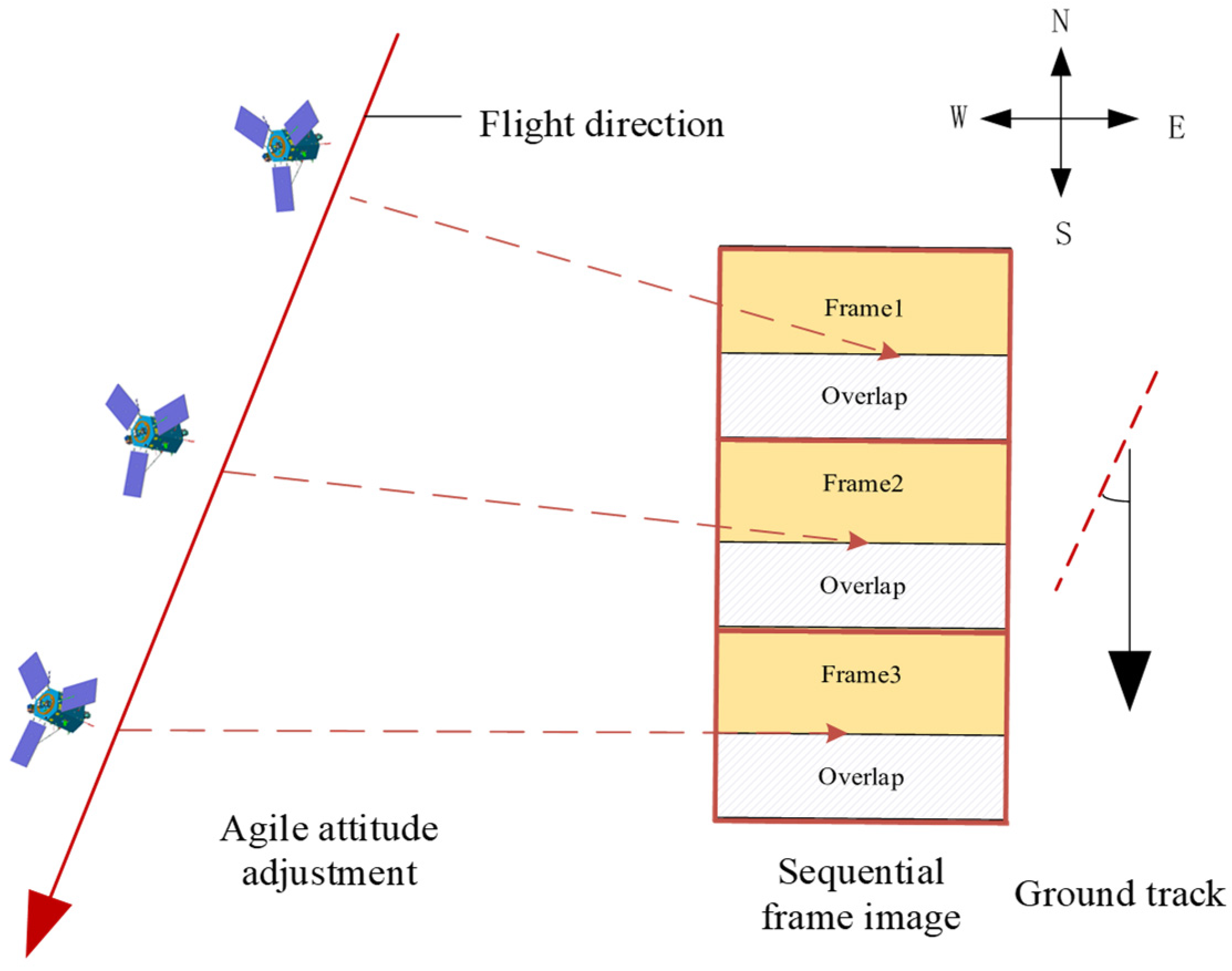
2.1. Sequential Frame Relative Orientation

For the relative misalignment problem in the frame imaging of LuoJia3-01, this study proposes a strategy of frame-by-frame adjustment compensation. During the process of relative orientation of sequential imagery, frame_i-1 is initially used as the reference frame, while frame_i serves as the compensation frame. Relative orientation is performed on frame_i, and its RPC is compensated. Subsequently, the compensated frame_i becomes the new reference frame, and frame_i+1 acts as the compensation frame for the next step. Relative orientation is then performed on frame_i+1, and its RPC is compensated accordingly. This process is reiterated until the last frame, and the entire processing flow is completed. The main process of this method is shown in Figure 3. In this process, image matching is used to obtain the initial matching points between the reference frame and the frame to be compensated, and global motion consistency constraints are used to eliminate mismatching points. This frame-by-frame adjustment orientation method ensures geometric consistency across sequential images, effectively addressing inter-frame misalignment issues and significantly enhancing the relative geometric accuracy of strip products.

2.1.1. Connection Point Matching and Gross Error Elimination

ORB (Oriented FAST and Rotated BRIEF) is a feature point description algorithm that combines the advantages of the FAST (Features from Accelerated Segment Test) key point detection algorithm and the BRIEF (Binary Robust Independent Elementary Features) descriptor algorithm [35]. The ORB algorithm exhibits certain rotation and scale invariance, with its greatest advantage over algorithms such as SIFT and SURF being its fast detection speed. Adjacent frame images exhibit some changes in the along-track direction, cross-track direction, and rotation, necessitating the use of a robust feature detection method for matching points. Considering that LuoJia3-01 frame imaging can capture two frames per second, and after relative radiometric correction, the inter-frame images are basically consistent in lighting, scale, and perspective, which makes ORB robust. Therefore, to meet near-real-time processing and high-precision requirements, this study uses the ORB feature matching algorithm for inter-frame point matching. Considering that this module has a high load and parallelism, the cudafeatures2d module of Opencv3.4.16 can be directly used for GPU-accelerated processing (Opencv: https://opencv.org/, accessed on 1 March 2024).

In the push-frame imaging process, adjacent frames have a large overlap, and most of the objects in the overlap area are relatively static. However, there may still be moving vehicles and ships, as well as other moving targets. Additionally, when shooting at an angle in areas such as those with tall buildings or mountains, there may be the phenomenon of perspective shift, resulting in “inaccurate matching point pairs”, which affect the accuracy of matching.

Therefore, the constraint of global motion consistency can be described as follows: the vector directions and lengths of all correctly matched point pairs should fall within a certain range, allowing us to infer that all correct matches also satisfy the property of having the same offset direction and distance, as shown in Equation (1):

$$\{\begin{array}{l}d{x}_k=x_I^k-x_J^k\\ d{y}_k=y_I^k-y_J^k\\ -{\delta }_{dxy}\le d{x}_k\le {\delta }_{dxy}\\ -{\delta }_{dxy}\le d{y}_k\le {\delta }_{dxy}\end{array}$$

(1)

Here, $\left(x_I^k,y_I^k\right)$ and $(x_J^k,y_J^k)$ represent the matched point pairs in the reference frame image and the compensated frame image, $d{x}_k \mathrm{a}\mathrm{n}\mathrm{d} d{y}_k$ are the relative errors in the x and y directions between the point to be compensated and the corresponding matched point in the reference frame image, and ${\delta }_{dxy}$ represents the mean square error of the residuals. Among the matched homologous points, the points with residual distribution exceeding the ${\delta }_{dxy}$ are eliminated, and the remaining points are the correct homologous points after gross error elimination.

2.1.2. Constructed Orientation Model Based on the RFM

The RFM is a mathematically simple model capable of achieving approximately the same level of accuracy as strict imaging models. Its RPC coefficients can be used to describe the deformations caused by factors such as optical projection, earth curvature, atmospheric transmission errors, and camera distortions. The RFM does not require consideration of the specific physical imaging process, making it highly accurate, computationally efficient, and sensor-independent. It is a standard geometric imaging model for remote sensing data products, especially suitable for regional network adjustment processing.

The RFM establishes a relationship between the object–space coordinates (latitude, longitude, and height) of a ground point and its corresponding image point coordinates (row and column) using ratio polynomials. To enhance the stability of parameter estimation, it is common to normalize the ground coordinates and image coordinates to a certain range as follows:

$$\begin{gathered} \{\begin{array}{c}{\displaystyle \frac{l-lineoff}{linescale}}={\displaystyle \frac{Nu{m}_L(X,Y,Z)}{De{n}_L(X,Y,Z)}}\\ {\displaystyle \frac{s-sampoff}{sampscale}}={\displaystyle \frac{Nu{m}_S(X,Y,Z)}{De{n}_S(X,Y,Z)}}\end{array}\{\begin{array}{l}X={\displaystyle \frac{lon-lonoff}{lonscale}}\\ Y={\displaystyle \frac{lat-latoff}{latscale}}\\ Z={\displaystyle \frac{h-heioff}{heiscale}}\end{array} \\ \{\begin{array}{l}Nu{m}_L(X,Y,Z)=a_i{X}^u{Y}^v{Z}^w(0\le i\le 19,u+v+w\le 3)\\ De{n}_L(X,Y,Z)=b_i{X}^u{Y}^v{Z}^w(0\le i\le 19,u+v+w\le 3)\\ Nu{m}_S(X,Y,Z)=c_i{X}^u{Y}^v{Z}^w(0\le i\le 19,u+v+w\le 3)\\ De{n}_S(X,Y,Z)=d_i{X}^u{Y}^v{Z}^w(0\le i\le 19,u+v+w\le 3)\end{array} \end{gathered}$$

(2)

Here, $a_i,b_i,c_i$ is the parameter of RFM and (X, Y, Z) represent the normalized object–space coordinates of the ground point. The purpose of normalization is to ensure the stability of the calculations. The parameters lineoff, sampoff, and lonoff, latoff, and heioff represent the normalization offsets for the image–space and object–space coordinates, respectively. Similarly, linescale, sampscale, and lonscale, latscale, and heiscale are the scale normalization parameters for the image–space and object–space coordinates.

Given the approximate parallel projection characteristics of the LuoJia3-01 push-frame imaging system, and despite the numerous and complex sources of imaging errors, the affine transformation can be used to describe the image–space distortion errors with a high accuracy between adjacent frames. Therefore, the mathematical model for block adjustment based on the RFM can be expressed as follows:

$$\{\begin{array}{l}l+\Delta l=RF{M}_x(lon,lat,h)\\ s+\Delta s=RF{M}_y(lon,lat,h)\end{array}$$

(3)

In Equation (3), l and s denote the row and column coordinates of the image point, $\mathsf{\Delta }l$ and $\mathsf{\Delta }s$ represent the image distortion errors, (lon, lat, h) are the corresponding object space coordinates, and x and y represent the across-track and along-track direction, respectively.

After the rigorous on-orbit geometric calibration and sensor correction processing of satellite imagery, geometric errors such as high-order camera lens distortions and atmospheric refraction are effectively corrected. As a result, the geometric errors in single-scene 1A image products are mainly low-order linear errors. Therefore, the affine transformation model can be selected as the additional image–space models Δl and Δs, which can be expressed as Equation (4):

$$\{\begin{array}{l}\Delta l=a_0+a_{1}l+a_{2}s\\ \Delta s=b_0+b_{1}l+b_{2}s\end{array}$$

(4)

Here, the parameter $a_0$ is used to absorb errors in the image’s across-track direction that are caused by position and attitude errors in the sensor’s scanning direction, while the parameter $b_0$ is employed to absorb errors in the image’s along-track direction resulting from position and attitude errors in the sensor’s flight direction. The parameters $a_2$ and $b_1$ will absorb image errors induced by GPS drift errors, and the parameters $a_1$ and $b_2$ will absorb image errors arising from internal orientation parameter errors.

2.1.3. Re-Calculation of RFM for the Compensation Frame

Based on building the inter-frame motion model and RFM orientation model, the relative orientation model of the compensation frame is constructed according to Equation (5), thereby achieving the mutual correspondence of coordinates between the sequence reference frame and the compensation frame:

$$\{\begin{array}{l}{x}_{i-1}=RF{M}_{i-1}^x(lon,lat,h)\\ y_{i-1}=RF{M}_{i-1}^y(lon,lat,h)\\ x_i+a_0+a_1\times x_i+a_2\times y_i=RF{M}_i^x(lon,lat,h)\\ y_i+b_0+b_1\times x_i+b_2\times y_i=RF{M}_i^y(lon,lat,h)\end{array}$$

(5)

Here, i − 1 denotes the reference frame in the sequence, and i denotes the compensated frame in the sequence. $(x_{i-1},y_{i-1})$ represents the image point on the reference frame, while $(x_i,y_i)$ represents the image point on the compensated frame. The points $(x_{i-1},y_{i-1})$ and $(x_i,y_i)$ form a pair of homologous points, and their object space coordinates are both (lon, lat, h). $RF{M}_x$ and $RF{M}_y$ represent the image point coordinates computed by the RFM in the row and column directions, respectively. The parameters $a_0, a_1, a_2, b_0, b_1, b_2$ are derived from Equation (4).

Taking into account that the orbit altitude of the LuoJia3-01 satellite is 500 km, the push-frame imaging frame rate is 2 frames/s, the satellite’s flight speed is 7 km/s, and the convergence angle between the reference frame and the compensated frame is only about 0.39°. If the traditional regional network adjustment method is used to solve the relative orientation parameters, the small convergence angle may cause the elevation error to be abnormally amplified, leading to the non-convergence of the adjustment. Therefore, this study introduces the DEM as an elevation constraint. The RPC solution for the compensated frame can be described as follows:

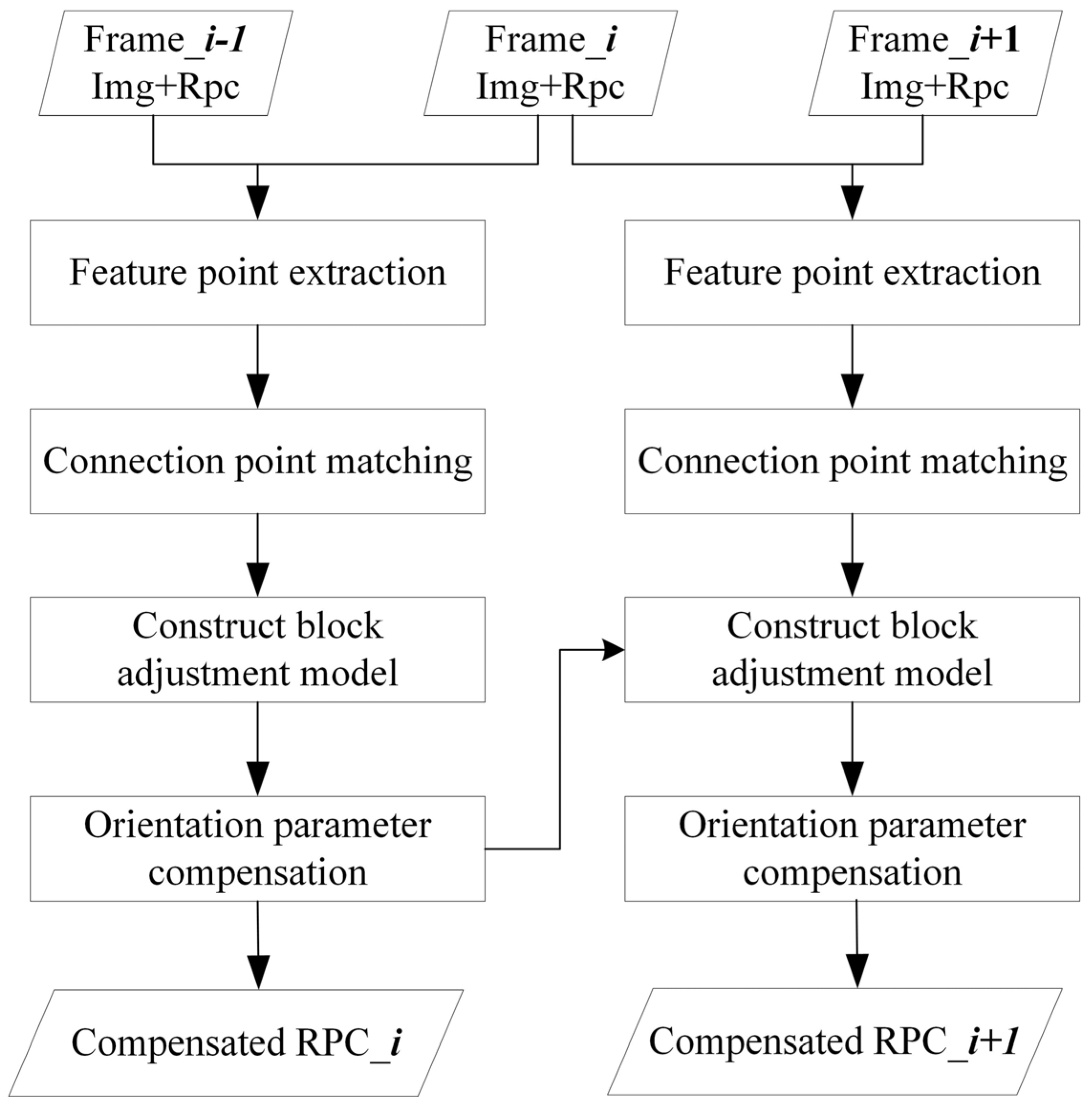
• In Section 2.1.1, after eliminating gross errors, several homologous points are obtained. Using Equation (4) and the least squares algorithm, the motion compensation parameters between frames, namely (a0, a1, a2, b0, b1, b2), can be determined.
• Based on the inter-frame motion parameters and the reference frame’s RPC, the inter-frame orientation model is constructed according to Equation (5).
• The compensation frame image is divided into a grid with a certain interval, resulting in uniformly distributed grid points. These points serve as virtual control points. Each virtual control point in the compensation frame is mapped to the reference frame and then projected onto the DEM to obtain the object–space point (lon, lat, h).
• This allows us to determine the image–space coordinates (s, l) and the object–space coordinates (lon, lat, h) for each virtual control point in the compensation frame. Subsequently, the terrain-independent method [16] can be utilized to calculate the high-precision RPC for the compensation frame.

2.2. Long-Strip Image Geometric Correction

The key to geometric correction in strip imaging is to establish a transformation model between the corrected strip image and the original sub-image coordinates, thereby achieving coordinate mapping from the original sub-image to the corrected strip image. During the frame imaging process, it is difficult to directly model the corrected strip image using strict models or rational functions. In the object coordinate system, each frame sub-image and the stitched large image have consistent geometric constraints. Therefore, in this study, a physical object stitching model is proposed to build a virtual plane. In the push-frame sequence imagery, since images separated by several frames (not exceeding 15) exhibit a certain degree of overlap, we can select a specific inter-frame interval for stitching and correction processes. For instance, in this study, an inter-frame interval of 10 was chosen, meaning that during processing, we focused on frame indices 1, 11, 21, …, 51, 61, significantly reducing the computational load of the data. As shown in Figure 4, the sub-images are divided into blocks in the object coordinate system and projected onto the object stitching virtual plane using a perspective transformation model. This approach ensures coordinate mapping from individual frames to the strip image based on the geographic consistency constraints of the frames, thereby addressing the challenges of inter-frame processing with complex overlaps.

2.2.1. Construction of Virtual Object Plane

• Determination of Pixel Resolution for the Virtual Object Image.

As shown in Figure 5, assuming that the four corner points of a certain frame of imagery are $P_0,P_1,P_2, \mathrm{a}\mathrm{n}\mathrm{d} P_3$, their corresponding object–space coordinates $\left(lo{n}_k,la{t}_k\right) (k=0,1,2,3)$ can be calculated using the RFM. The pixel-based latitude and longitude resolutions in the cross-track and along-track directions can then be determined using Equations (6) and (7).

In Equation (6), the lon-resolution $pgs{d}_{x0}$ of the first row was computed based on the latitude and longitude positions of points P0–P1, and the pixel distance between them. Similarly, the lon-resolution $pgs{d}_{x1}$ of the last row is determined as P2–P3 points. The average of these two values $pgs{d}_x$ is used as the lon-resolution for this frame of the image.

$$\{\begin{array}{l}pgs{d}_{x0}=\sqrt{{(lo{n}_1-lo{n}_0)}^2+{(la{t}_1-la{t}_0)}^2}/\sqrt{{(x_1-x_0)}^2+{(y_1-y_0)}^2}\\ pgs{d}_{x1}=\sqrt{{(lo{n}_3-lo{n}_2)}^2+{(la{t}_3-la{t}_2)}^2}/\sqrt{{(x_3-x_2)}^2+{(y_3-y_2)}^2}\\ pgs{d}_x=(pgs{d}_{x0}+pgs{d}_{x1})/2\end{array}$$

(6)

Similarly to the process for calculating the lon-resolution of the frame image, the lat-resolution of the frame image can be computed according to Equation (7).

$$\{\begin{array}{l}pgs{d}_{y0}=\sqrt{{(lo{n}_2-lo{n}_0)}^2+{(la{t}_2-la{t}_0)}^2}/\sqrt{{(x_2-x_0)}^2+{(y_2-y_0)}^2}\\ pgs{d}_{y1}=\sqrt{{(lo{n}_3-lo{n}_1)}^2+{(la{t}_3-la{t}_1)}^2}/\sqrt{{(x_3-x_1)}^2+{(y_3-y_1)}^2}\\ pgs{d}_y=(pgs{d}_{y0}+pgs{d}_{y1})/2\end{array}$$

(7)

In this way, for a strip sequence image containing n count frames, the resolutions of latitude and longitude in the across-track and along-track directions of the stitched image points can be represented as $gs{d}_x$ and $gs{d}_y$, respectively.

$$\{\begin{array}{l}gs{d}_x={\displaystyle \sum _{i=1}^n{(pgs{d}_x)}_i}/n\\ gs{d}_y={\displaystyle \sum _{i=1}^n{(pgs{d}_y)}_i}/n\end{array}$$

(8)

2.

Determination of the Projection Model for Object–Space Coordinates.

There are complex misalignment and overlap situations among the push-frame sequence images. Accurately calculating the range of the stitched virtual plane is the basis for subsequent geometric correction. Assuming that there are n frame images to be stitched, the latitude and longitude coordinates of the four corner points of each frame image are compared according to Equation (9) in order to find the maximum inscribed rectangle $T_0{T}_1{T}_2{T}_3$ (Figure 5) and the corresponding range of coordinates. This can accomplish the rapid processing of unaligned image frame edges, only outputting the quadrilateral of the effectively filled region.

$$\left\{\begin{array}{l}minLon=\mathit{max}\{(lo{n}_0,lo{n}_2{)}_1,(lo{n}_0,lo{n}_2{)}_2,...,(lo{n}_0,lo{n}_2{)}_n\}\\ maxLon=\mathit{min}\{(lo{n}_1,lo{n}_3{)}_1,(lo{n}_1,lo{n}_3{)}_2,...,(lo{n}_1,lo{n}_3{)}_n\}\\ minLat=\mathit{max}\{(la{t}_2,la{t}_3{)}_1,(la{t}_2,la{t}_3{)}_2,...,(la{t}_2,la{t}_3{)}_n\}\\ maxLat=\mathit{min}\{(la{t}_0,la{t}_1{)}_1,(la{t}_0,la{t}_1{)}_2,...,(la{t}_0,la{t}_1{)}_n\}\end{array}\right.$$

(9)

After determining the boundary range and latitude–longitude resolution of the virtual stitching plane, the image size (oWidth, oHeight) of the virtual plane and the object–space projection model (OPM) can be further determined.

$$\{\begin{array}{l}oWidth=(maxLon-minLon)/gs{d}_x\\ oHeight=(maxLat-minLat)/gs{d}_y\end{array}$$

(10)

The OPM refers to the use of an affine transformation model to describe the mapping relationship between the image–plane coordinates and the object–space latitude and longitude coordinates for stitched images that have undergone geometric correction.

$$\{\begin{array}{l}lon=minLon+gs{d}_x\times x,0\le x<oWidth\\ lat=maxLat+gs{d}_y\times y,0\le y<oHeight\end{array}$$

(11)

In Equation (11), $(x,y)$ represents the image–plane coordinates, and $(lon,lat)$ represents the object–space latitude and longitude coordinates.

2.2.2. Building a Block Perspective Transformation Model

The traditional geometric correction method is based on the OPM, RFM, and DEM; it establishes a transformation relationship between the output image object–space coordinates and the input image pixel coordinates pixel by pixel, and then it resamples the input image. If the RFM is used to convert between image coordinates and object coordinates point by point, then the computation will be enormous. Therefore, this study proposes a coordinate mapping strategy based on the block perspective transformation model (BPTM) to significantly reduce the complexity of the calculation while ensuring accuracy. In this method, the original image is first divided into grids, and few virtual control points are uniformly divided within the grids. Within each grid, only the virtual control points are solved for their object coordinates based on the RFM and DEM, and their image coordinates in the stitched image are calculated according to the OPM. In this way, by using a certain number of control points within each grid, a direct mapping relationship between the original image pixel coordinates and the stitched image pixel coordinates can be determined using the least squares algorithm.

$$\{\begin{array}{l}x={\displaystyle \frac{a_{0}s+a_{1}l+a_2}{a_{3}s+a_{4}l+1}}\\ y={\displaystyle \frac{a_{5}s+a_{6}l+a_7}{a_{3}s+a_{4}l+1}}\end{array}$$

(12)

Here, $s$ and $l$ are the input image pixel plane coordinates; $x$ and $y$ are the output image pixel plane coordinates; and $a_0-a_7$ are the parameters of the perspective transformation model.

The perspective transformation model contains eight parameters, and, by using the four corner points of the divided grid, eight equations can be formulated for solving. In order to ensure the reliability of the solution, uniform sparse control points are further divided inside the grid to construct adjustment observation equations, as shown in Equation (13).

$$\{\begin{array}{l}{v}_x=a_{0}s+a_{1}l+a_2-x{a}_{3}s-x{a}_{4}l-x\\ v_y=a_{5}s+a_{6}l+a_7-y{a}_{3}s-y{a}_{4}l-y\end{array}$$

(13)

In this way, a least squares equation can be constructed and the unknown parameters $a_0-a_7$ can be solved, as shown in Equation (14).

$$\{\begin{array}{l}AX=L\\ X=(A^{T}A{)}^{-1}{A}^{T}L\end{array}$$

(14)

Here,

$$\begin{gathered} A=\left[\begin{array}{cccccccc}{s}_1& l_1& 1& -x_1\ast s_1& -x_1\ast l_1& 0& 0& 0\\ 0& 0& 0& -y_1\ast s_1& -y_1\ast l_1& s_1& l_1& 1\\ & & & \dots & & & & \\ s_n& l_n& 1& -x_n\ast s_n& -x_n\ast l_n& 0& 0& 0\\ 0& 0& 0& -y_n\ast s_n& -y_n\ast l_1& s_n& l_n& 1\end{array}\right] \\ X={\left[\begin{array}{cccccccc}{a}_0& a_1& a_2& a_3& a_4& a_5& a_6& a_7\end{array}\right]}^T \\ L={\left[\begin{array}{ccccc}{x}_1& y_1& \dots & x_n& y_n\end{array}\right]}^T \end{gathered}$$

(15)

In Equations (14) and (15), ${(s,l)}_i$ and ${(x,y)}_i$ are the i-th virtual control points, the number of points of which is n. A, X, and L form the adjustment observation equation, where A is the design matrix, L is the vector of observed values, and X represents the vector of unknown parameters.

2.2.3. Image Point Densified Filling (IPDF) and Coordinate Mapping

The push-frame imaging sequence has a high degree of overlap, with more than a dozen frames covering the same area. If indirect correction methods are used for multi-frame correction and geometric stitching, all pixels in the overlapping area need to be selected and matched in the original multiple frames during the coordinate transformation process, which greatly reduces the efficiency of processing.

Direct methods can effectively solve this problem, but they also face the issue of missing pixels in the corrected images, requiring the reassignment of grayscale values. Therefore, it is proposed to ensure that the corresponding grayscale values are covered within the corrected image area by densifying the original image pixels. An IPDF grid size $W$ is set by Equation (16), which depends on the ratio of the maximum spatial resolution $gs{d}_{max}$ to the minimum spatial resolution $gs{d}_{min}$ of all pixels in a single frame image, and independent of ground features and terrain.

$$W=(\mathrm{int})({\displaystyle \frac{gs{d}_{\max }}{gs{d}_{\min }}}+0.5)$$

(16)

where $\mathrm{i}\mathrm{n}\mathrm{t}$ denotes the integer rounding operation. Since Luojia3-01’s spatial resolution of pixels at different locations in the original image is nearly identical, only a size of (W = 2) is required in both the across-track (x) and along-track (y) directions at the IPDF point process.

$$\{\begin{array}{l}{P}_{i,x}=x+i/W,0\le i<W\\ P_{i,y}=y+j/W,0\le j<W\end{array}$$

(17)

Assuming a certain point $P(x,y)$ in the original image, four virtual points, P1, P2, P3, and P4, are generated through densification in the two-dimensional plane direction according to Equation (17). The grayscale values of the densified virtual points can be determined through bilinear interpolation from the original image. Based on this, Equation (12) is used to project the densified virtual points P1–P4 onto the virtual object–space plane. In this way, after one densification process of the original image, it can be ensured that each pixel in the output image has grayscale value coverage. However, this densification process increases the computational load four times, sacrificing the efficiency of the algorithm. An effective solution is to map it to the GPU for accelerated processing.

2.3. GPU Parallel Acceleration Processing

Although block perspective transformation effectively reduces the computational load of coordinate transformation, it also introduces an additional computational load for fitting transformation model parameters. Additionally, the amount of data after IPDF is increased significantly, and the computational load of resampling is not reduced. Therefore, the overall computational load of the correction and stitching process is still significant, requiring the use of GPU parallel processing technology to further enhance the execution efficiency of the method. This study chooses the mainstream unified device computing architecture (CUDA) as the GPU parallel processing framework, and it employs a “progressive” strategy for GPU parallel processing (Figure 6): first, through GPU parallel mapping, the kernel function execution flow and basic settings are clarified to ensure that the method can be executed on the GPU; then, through “two-level” performance optimization, the method’s execution efficiency on the GPU is further improved.

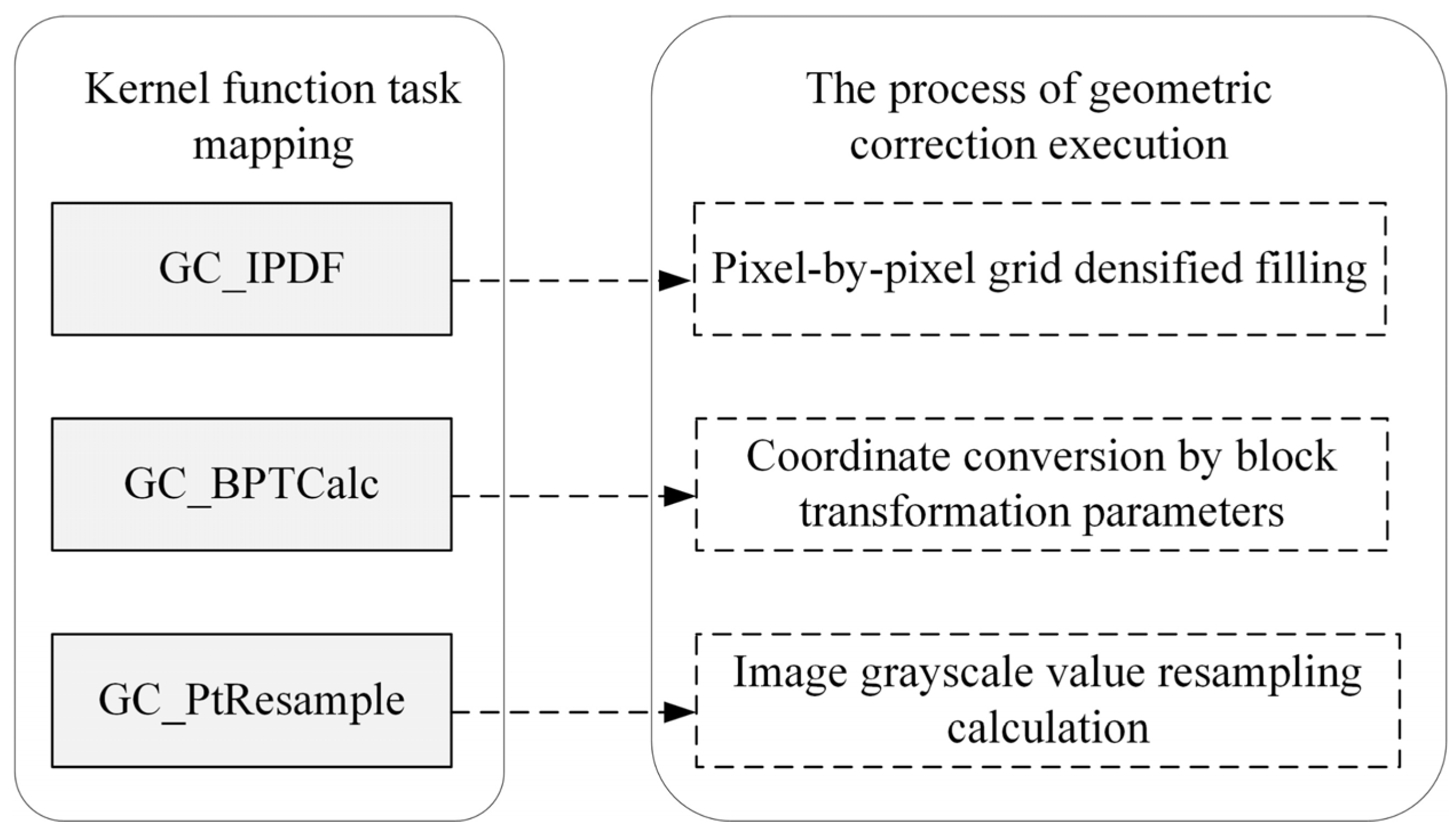
2.3.1. Kernel Function Task Mapping

First, kernel function task mapping is performed to determine the logical flow of geometric correction execution on the GPU. Since the pixel densified calculation, direct linear transformation calculation, and image resampling calculation are all grid-/pixel-independent, they have high parallelism. Therefore, based on the principle of maximum GPU parallel execution, the above three steps are mapped to the GPU for execution. Considering the logical continuity of the three steps, in order to reduce the additional overhead caused by repeated kernel function calls, the three steps are further mapped to three independent kernel functions: GC_IPDF, GC_BPTCalc, and GC_PtResample, as shown in Figure 6. Specifically, the GC_IPDF kernel function assigns each CUDA thread to densify pixel grids in the row and across-track directions; the GC_BPTCalc kernel function assigns each CUDA thread to calculate its coordinates in the original image and its pixel coordinates in the image to be stitched using the coordinate mapping parameters calculated by the CPU; and the PixelResample kernel function assigns each CUDA thread to utilize the pixels around the densified pixel in the original image, determine its grayscale value through bilinear interpolation, and fill it into the image to be stitched.

2.3.2. GPU Parameter Optimization Settings

Kernel function performance optimization mainly includes three parts: kernel function instruction optimization, thread block size, and storage hierarchy access.

• Kernel function instruction optimization: (1) As few variables as possible should be defined, and variables should be reused as much as possible to save register resources. (2) Sub-functions should be unrolled to avoid function call overhead. (3) Variables should be defined only when they are used to better adhere to the principle of locality, facilitating the compiler optimization of register usage. (4) The use of the branching and cycle code should be avoided if possible.
• Thread block size: (1) The size of the thread block should be at least 64 threads. (2) The maximum number of threads in a block cannot exceed 1024. (3) The size of the thread block should be a multiple of the number of thread warps (32 threads) to avoid meaningless operations on partially unrolled thread warps. In the kernel function, we set the number of threads in a block to 256 (16 pixels × 16 pixels), with each thread responsible for processing 1 pixel. Therefore, if the size of the image to be processed is width × height, [width/16] × [height/16] thread blocks are required to process the entire image (rounding up to ensure that all pixels are covered).
• Optimization of hierarchical memory access in storage: The CUDA architecture provides multiple levels of memory available to each executing thread. Arranged from top to bottom, they are registers, shared memory (L1 cache), L2 cache, constant memory, and global memory. As the level goes down, the capacity gradually increases, while the speed decreases. In the process of IPDF correction, the basic processing unit for a single thread is several adjacent pixels, and there is no need for interaction among the threads. The CUDA function “cudaFuncCachePreferL1” can be used to allocate on-chip shared memory to the L1 cache, optimizing thread performance. Parts of the algorithm that can be considered constants, such as RPC parameters and polynomial fitting parameters, which need to be concurrently read a large number of times during algorithm execution and only involve read operations without write operations, can be placed in constant memory to improve parameter access efficiency by leveraging its broadcast mechanism.

3. Results

3.1. Study Area and Data Source

This study selected four sets of LuoJia3-01 frame array push-frame data obtained at different times and locations; the specific information is shown in

Table 2. Detailed information of experimental data.

DataId	Image Time	Center Position	Attitude Angle (°)
			Roll	Pitch	Yaw
Data1	26 Feb 2023	E106.52_N29.54	−22.7~−16.2	13.4~−20.8	−7.6~−6.7
Data2	27 Feb 2023	E93.51_N42.780	−8.8~0.4	13.1~−24.9	−9.6~−9.3
Data3	10 Mar 2023	E89.20_N42.91	9.0~15.8	11.7~14.7	−10.6~−10.9
Data4	18 Mar 2023	E65.52_N44.61	−6.8~3.4	24.9~−15.0	−10.0~−9.95

. The spatial resolution of these data is 0.7 m, with the image size of a single frame being 7872 (cross-track) × 5984 (along-track) × 3 (bands) pixels. Each set of data contains 60 frames, with an imaging duration of 30 s. These data cover different scenes such as mountains, rivers, plains, and cities. The satellite travels at a speed of 7 km/s, which would theoretically result in the satellite covering a distance of 210 km. However, during the push-frame imaging process, the satellite performs agile maneuvers to extend the exposure time for each frame by continuously adjusting its attitude angles. This results in an effective speed along the flight direction of the camera image that is lower than the satellite speed. The overlap between adjacent frames is 90%, leading to a total effective image length of about 24 km. Considering the significant overlap in the sequence images, we select a frame interval with 10 for processing and presentation, as shown in Figure 7 (top-to-bottom direction). We can see that these data have complex overlaps between frames, which need to be corrected and stitched through algorithms to meet application requirements. The DEM required for the processing is the publicly available global ASTER DEM, which has an elevation accuracy of within 50 m and is sufficient to meet the elevation accuracy requirements for the geometric correction of push-frame strips.

3.2. Algorithm Accuracy Analysis

To verify the effectiveness of the algorithm in this study, three experimental schemes are designed for verification analysis.

E1: According to the sequence images of push-frame imaging and RPC parameter information, geometric correction is performed frame-by-frame, and then physical geometric stitching is carried out on this basis [24].

E2: Based on the sequence images of push-frame imaging and RPC, geometric correction is carried out frame-by-frame. On this basis, image registration is performed through ORB matching, and, finally, object–space geometric stitching is conducted [36].

E3: ORB feature extraction is carried out on the original image in the overlapped regions of adjacent frames, and reliable tie points are selected through global motion consistency. With the previous frame image as the reference frame and the following frame image as the main frame, RPC compensation is conducted. Based on the compensated RPC and original images, long-strip geometrically corrected images are generated according to the method in Section 2.2.

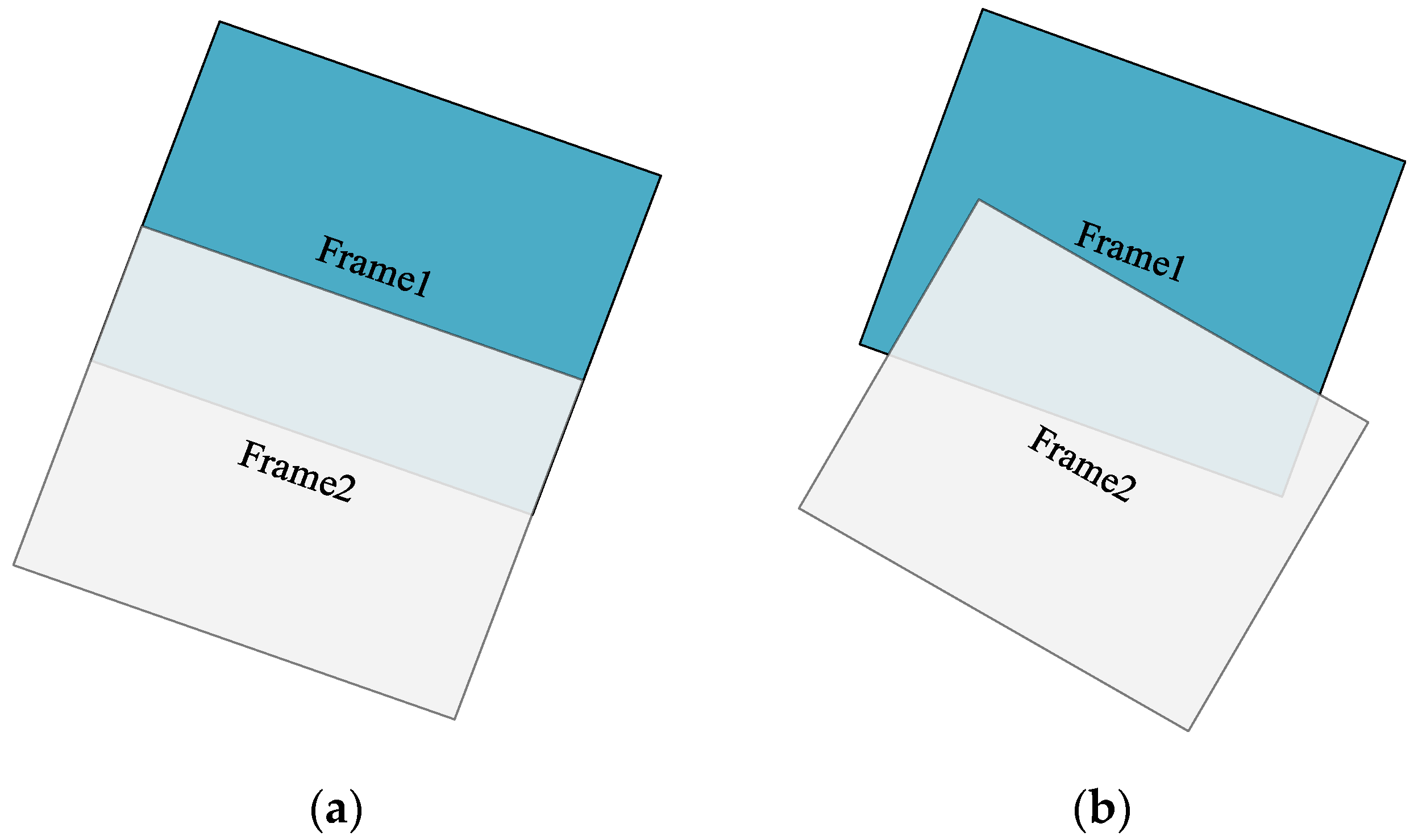
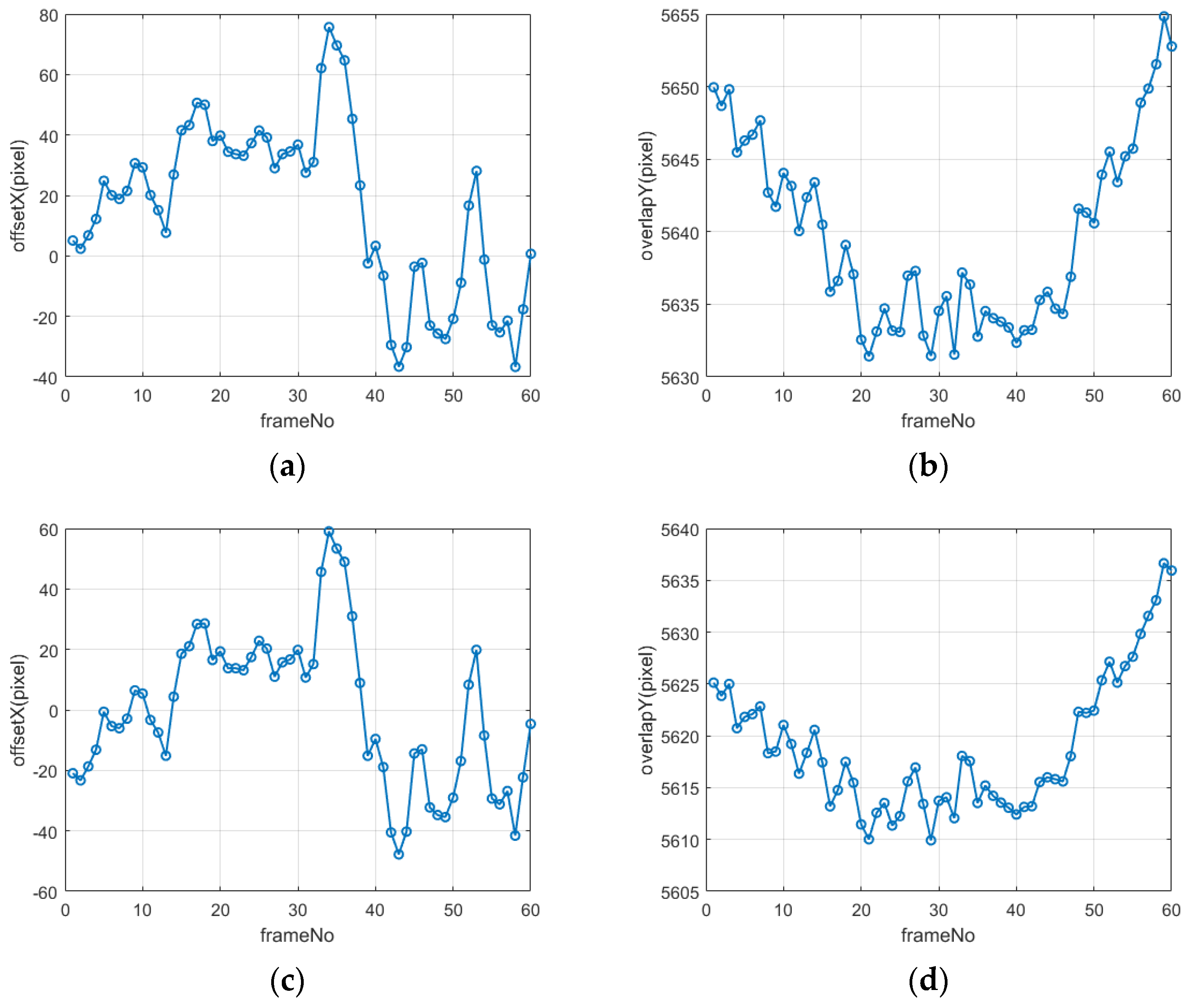
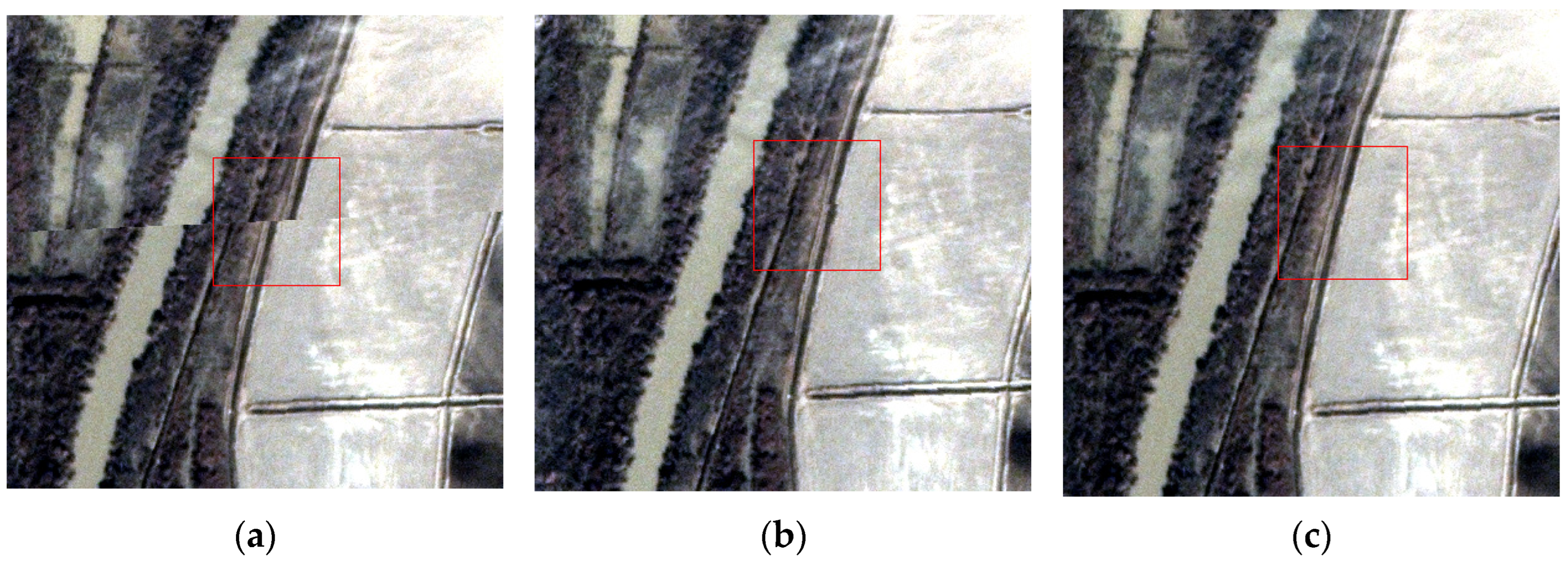
3.2.1. Analysis of Inter-Frame Image Misalignment

Analyzing the misalignment relationship between adjacent frames helps to further verify the platform jitter during the agile imaging process of LuoJia3-01. This is also the basis for subsequent inter-frame geometric stitching. We select the previous frame as the reference frame image and the following frame as the compensatory frame image. By calculating the row and column positions of the first and last pixels of the first row of the compensatory frame image in the reference frame image through object coordinate consistency, the number of overlapping rows in the track direction and the relative offset in the perpendicular track direction of the adjacent frame images can be roughly determined.

According to an analysis of the results in Figure 8, the number of overlapping rows in the track direction of adjacent frame images is between 5605 and 5655 rows. The number of overlapping rows varies significantly between different inter-frame images, and it also differs between different pixels in the same row. In the across-track direction, the offset between inter-frame images is between −60 and 80 pixels, and it changes non-systematically with the frame number. It can be foreseen that, in the push-frame imaging mode, in order to maintain nearly north–south vertical stripe imaging, the satellite needs to perform large attitude maneuvers in real time, resulting in the unstable imaging of the platform and a decrease in attitude measurement accuracy. This, in turn, causes the misalignment and distortion of the stripe images.

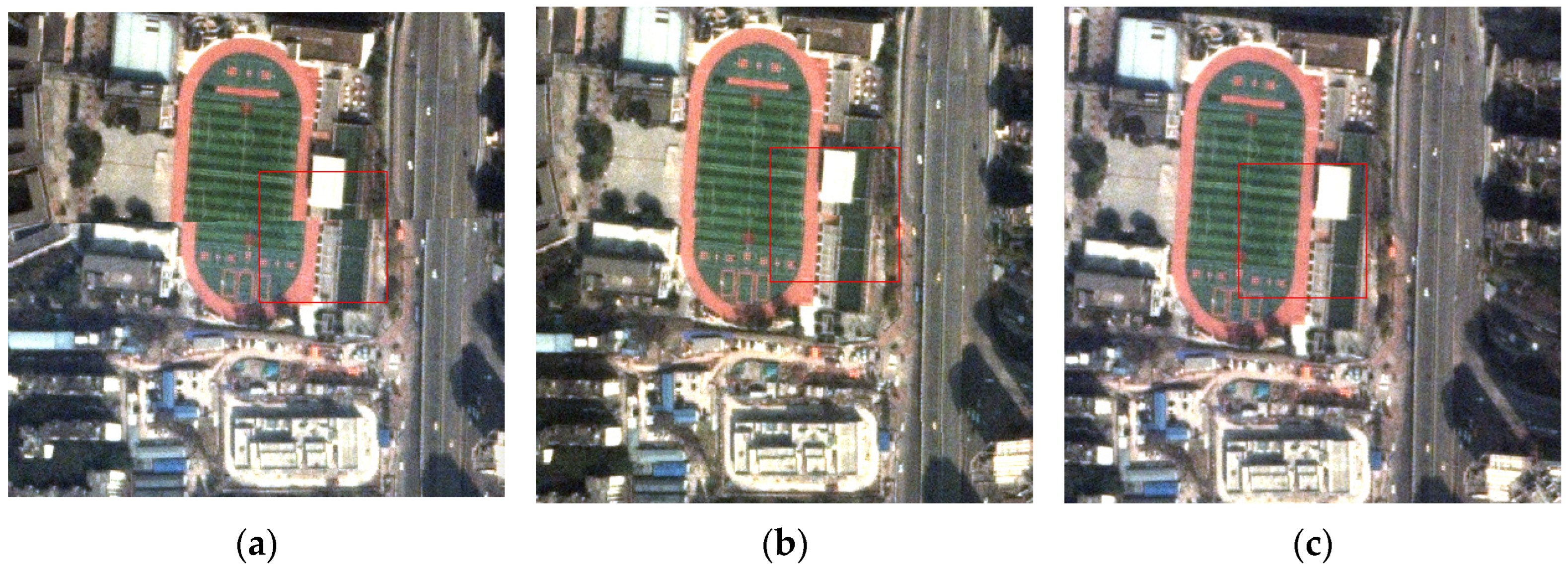
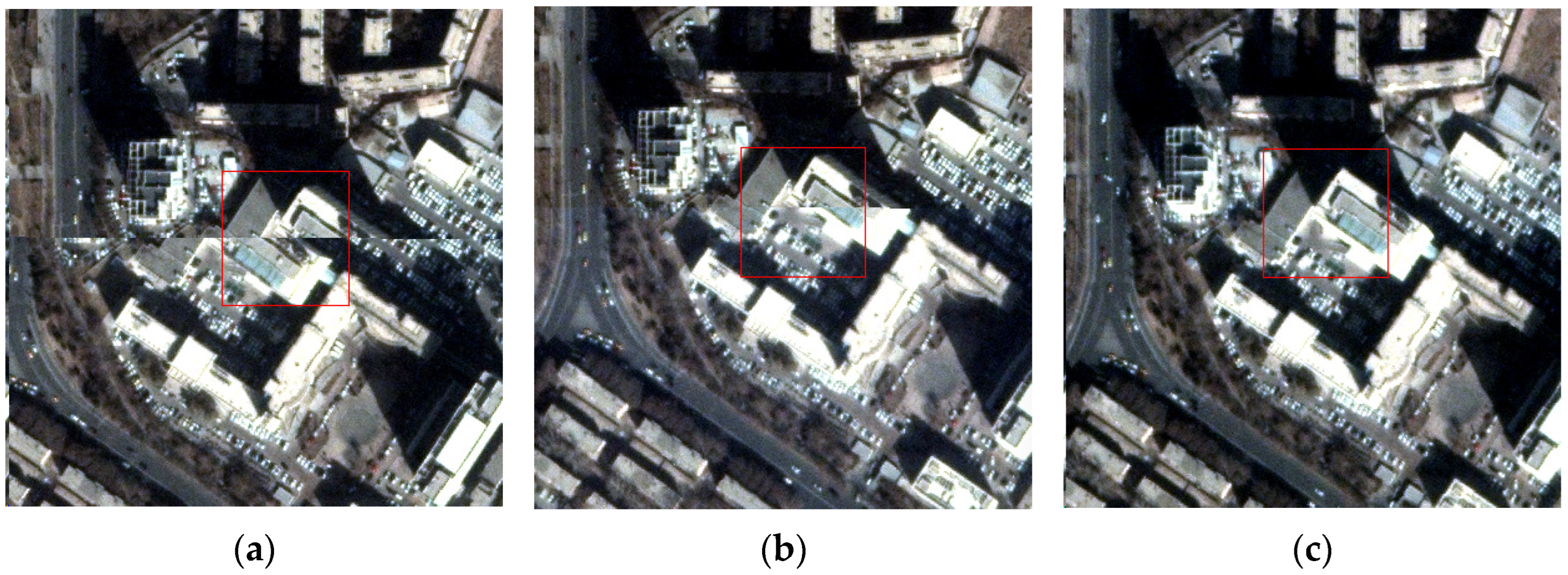
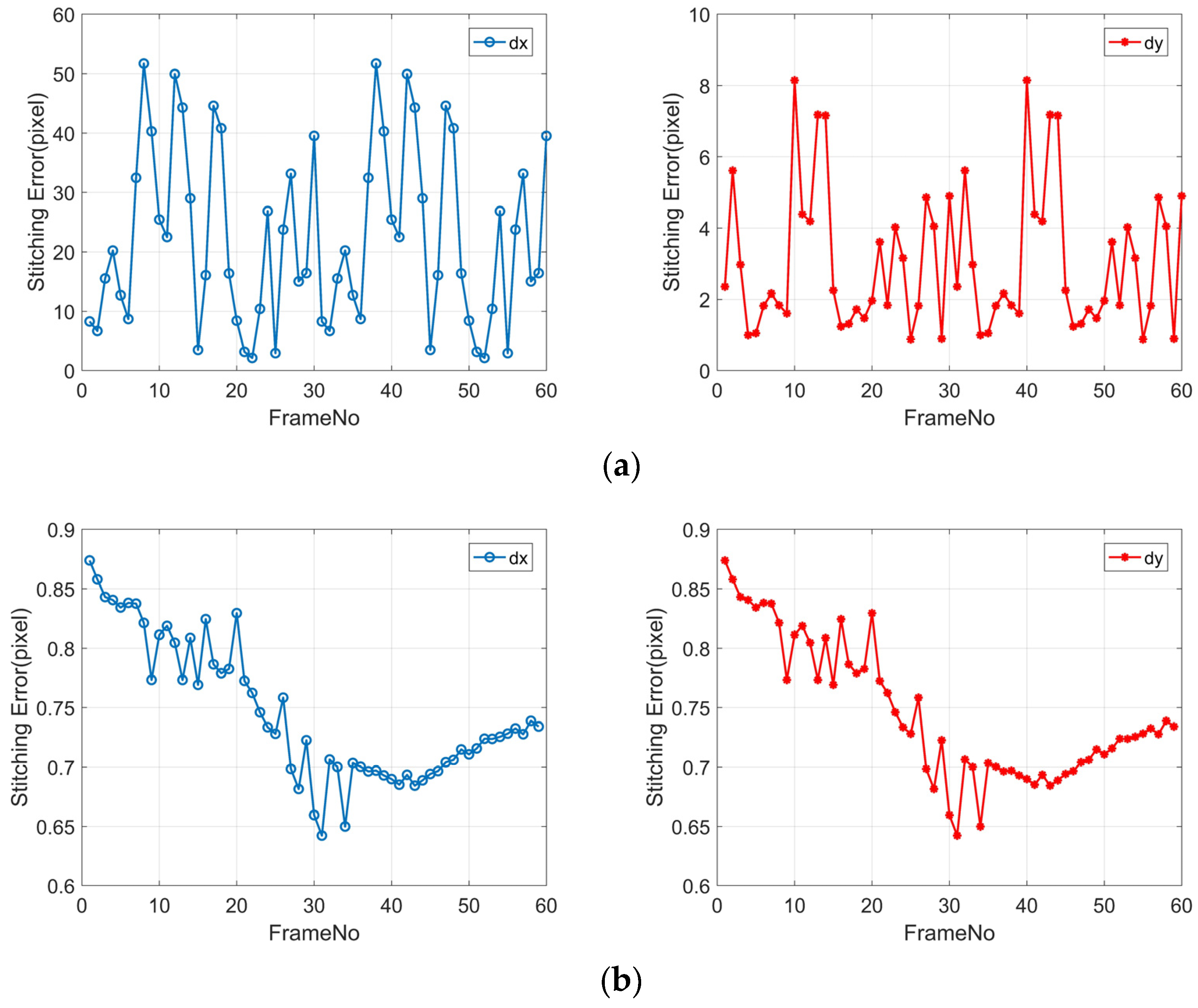
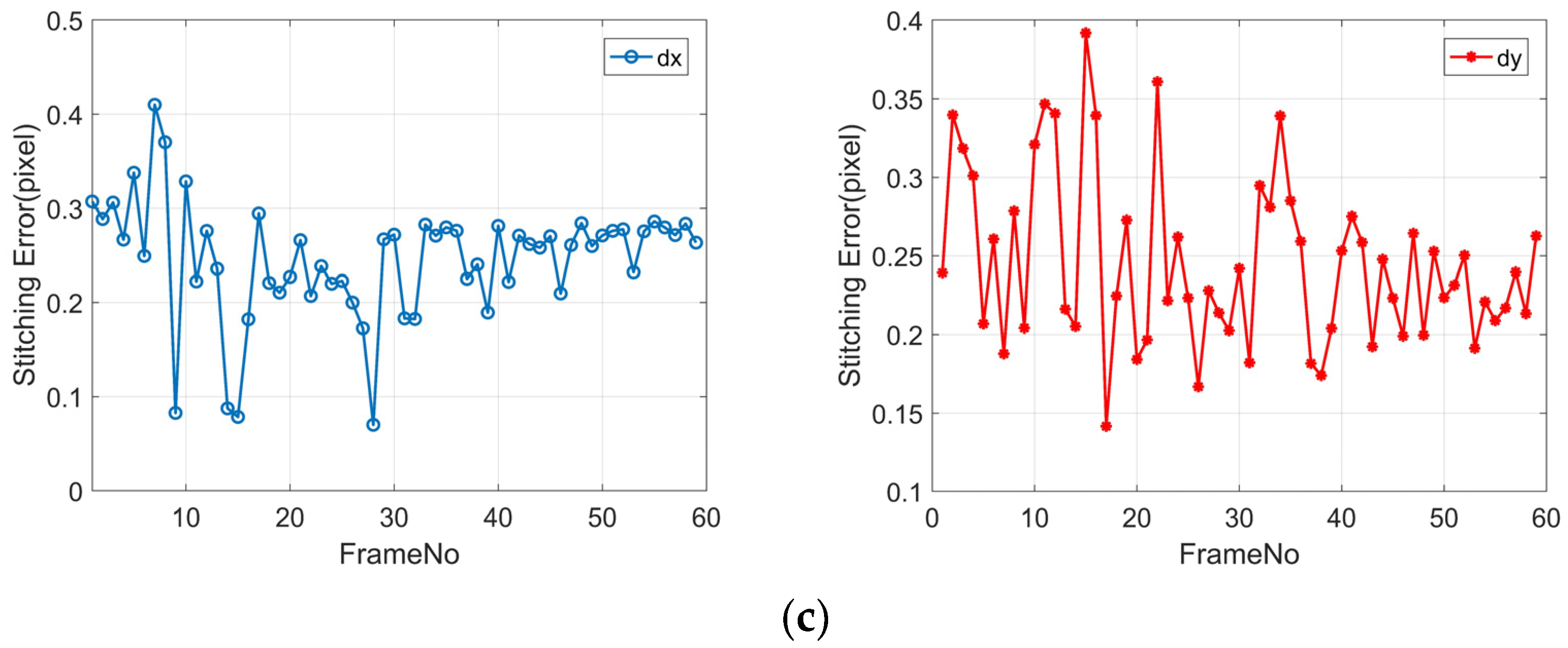
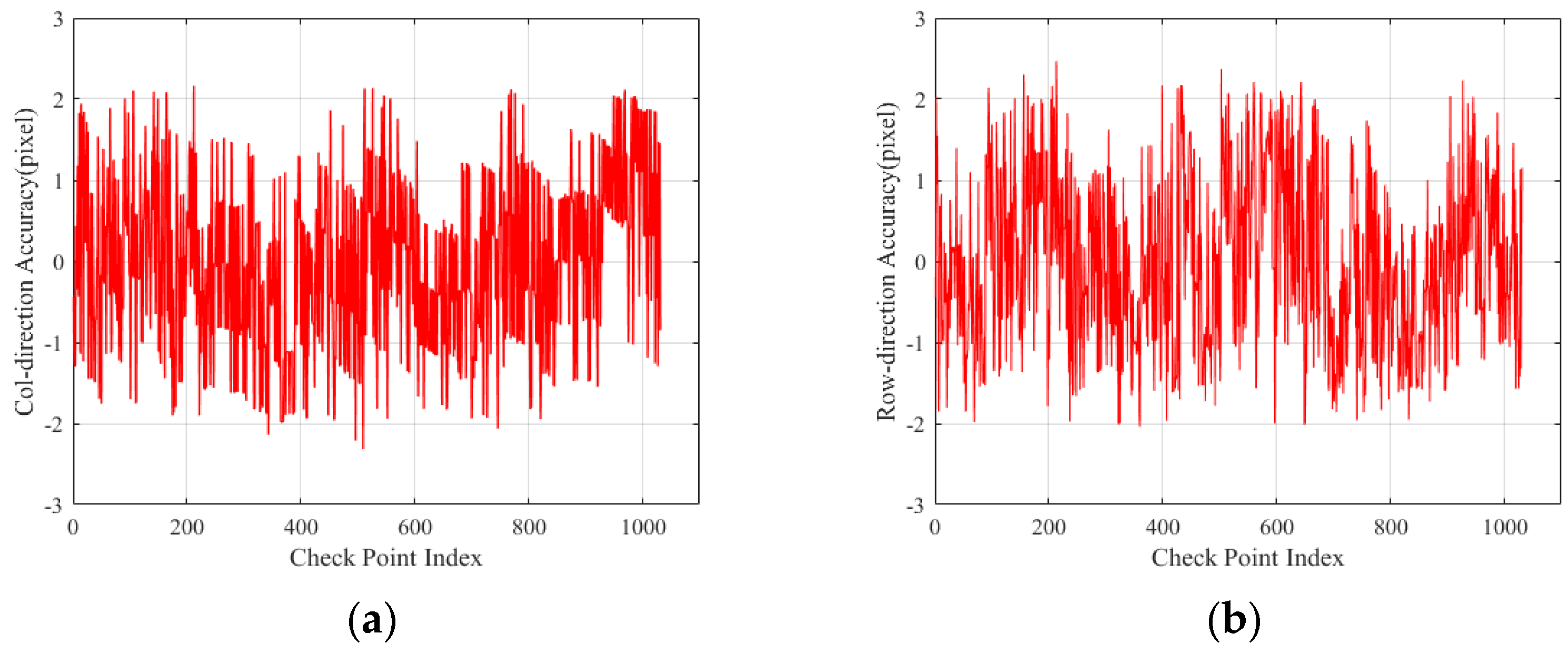
3.2.2. Analysis of Inter-Frame Registration Accuracy

The registration accuracy of adjacent images directly determines the geometric quality of the stitched image. Therefore, we project the adjacent frame images from the image space to the object space, and we conduct comparative experiments following the three test scenarios in Section 3.1, analyzing the registration effect of inter-frame images using visual and quantitative methods. The comparative test results of the four sets of data are shown in Figure 9, Figure 10, Figure 11 and Figure 12. In these result images, the first row shows local images with a 400 × 400 window, the second row shows the magnified results of the red box area, and panels (a–c) present the results corresponding to experiments E1/E2/E3, respectively.

It can be observed that there is a significant geometric misalignment in the inter-frame images in E1, reaching tens of pixels. The E2 results show almost imperceptible overall misalignment, but there are subtle misalignments in the further local magnification window. After processing with the algorithm in this study, E3 achieves precise registration and the seamless geometric stitching of inter-frame images.

In order to further quantitatively analyze the reliability of inter-frame registration accuracy, dense matching was performed on overlapping images of adjacent frames to calculate the relative accuracy of the same-name matching points as the registration accuracy evaluation index. The experiment selected data1 data for the inter-frame registration accuracy analysis according to the three experimental schemes E1/E2/E3, and the results are shown in Figure 13.

Due to the lack of compensation for the relative differences in exterior orientation elements between the inter-frame images in E1, there is a registration error of more than 50 pixels in the cross-track direction and over 8 pixels in the along-track direction. These results arise because the satellite platform’s stability during push-frame agile imaging introduces random errors, with a maximum deviation of up to 0.005°. Additionally, errors from time synchronization and attitude interpolation contribute to this issue. Consequently, if RPCs are generated directly from the original geometric imaging model for positioning, the maximum inter-frame relative error can reach over 50 pixels.

In E2, image registration is performed based on geometric correction, significantly reducing inter-frame registration errors, with a planar error of around 1 pixel. The image registration accuracy of the results from E2 is relatively low, likely due to inaccurate terrain changes, sensor measurement errors, and errors in control point distribution introduced during geometric correction, making it difficult to perform image registration through a global transformation model. E3 has registration accuracies better than 0.5 pixels in the along-track, nadir, and planar directions, as it utilizes L1A-level images before geometric correction and corrects relative errors on the image plane caused by attitude errors through global affine transformation. These results indicate that conducting geometric stitching based on relative orientation is feasible, and the inter-frame registration accuracy can meet the requirements for seamless geometric stitching.

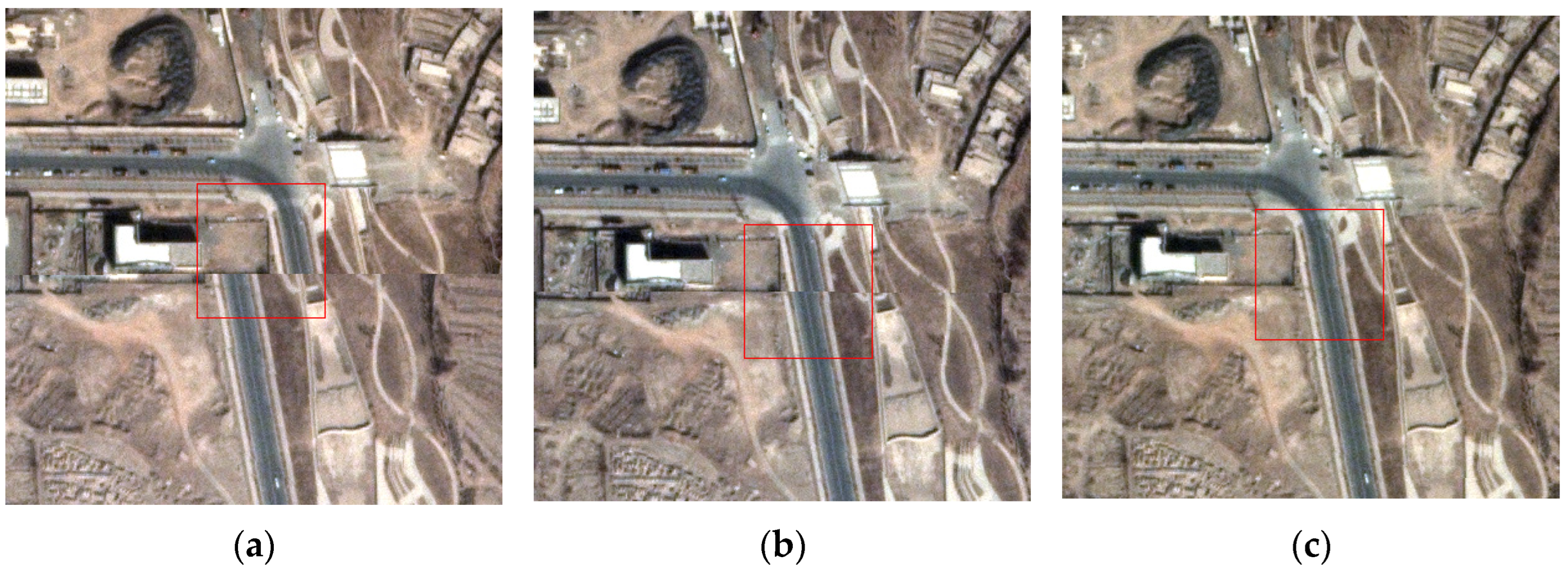
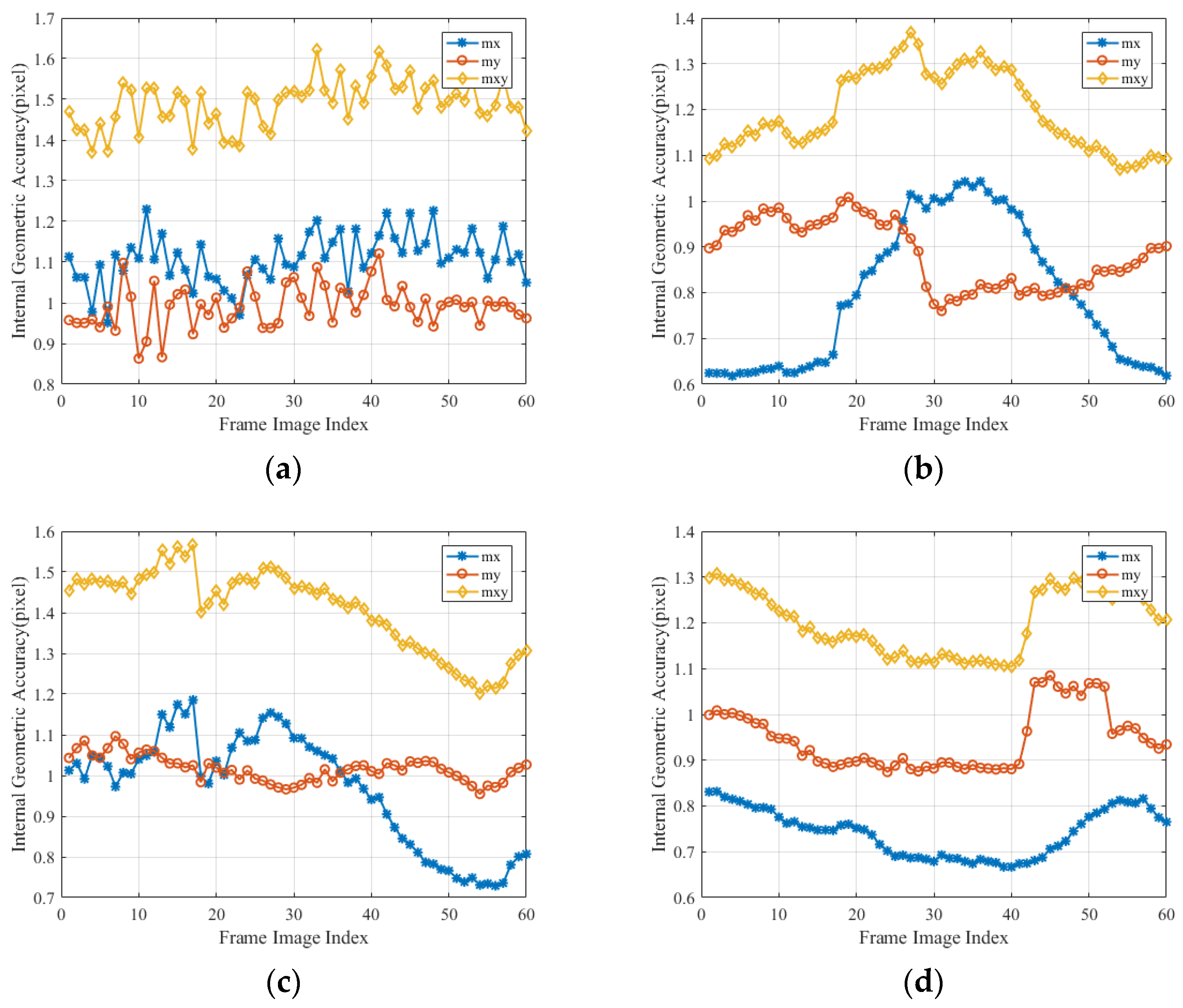
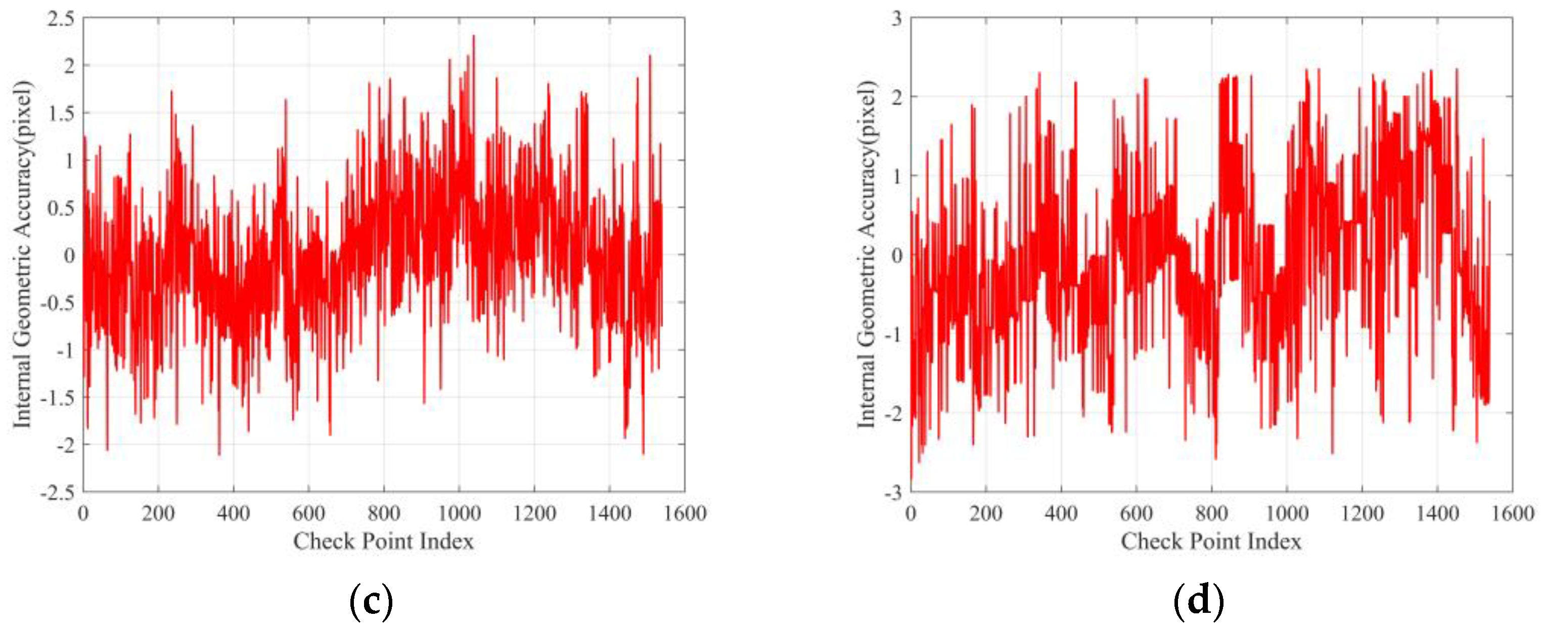
3.2.3. Analysis of Strip Geometric Correction Images’ Internal Geometric Accuracy

A strip geometric correction product is generated through sequential frame image geometric correction and stitching. Its geometric internal accuracy can well reflect the relative geometric accuracy between frames. Figure 14 shows the overall stitching results of all data under different experimental methods. Due to the inaccuracies in satellite attitude measurements during agile imaging, we can see that, in Figure 14a,b, the stitching results of the sequence frame images exhibit approximate north–south vertical stripes, with distorted deformation at the edges of the stitched images, and the degree of inter-frame misalignment and deformation undergo non-systematic changes with the image row coordinate position. It can also be observed that, within adjacent frame images, there are cross-track direction offsets, along-track direction offsets, and relative rotation amounts, consistent with the inter-frame misalignment caused by the previously analyzed attitude angle errors, severely affecting the data application. After processing with our method E3, very good visual stitching results are achieved, as shown in Figure 14c, effectively eliminating misalignment and cropping the image’s black edges that are not aligned.

The internal geometric accuracy of the image is determined by calculating the statistical values of the relative errors between the checkpoints in the image, reflecting the magnitude of non-linear errors within the image. As show in Equation (16), $X_{Oi}$ and $Y_{Oi}$ are the positioning errors in the x-direction (across-track direction) and y-direction (along-track direction) for the i-th checkpoint, and the average value of the absolute positioning errors of all checkpoints is selected as the reference error. For $n-1$ checkpoints, the mean errors $m_x$, $m_y$, and $m_{xy}$ are calculated in the x-direction, y-direction, and plane direction, respectively.

$$\left\{\begin{array}{l}{m}_x=\sqrt{{\displaystyle \sum _{i=1}^{n-1}}(X_{Oi}-{\stackrel{̑}{X}}_O{)}^2/n-1}\\ m_y=\sqrt{{\displaystyle \sum _{i=1}^{n-1}}(Y_{Oi}-{\stackrel{̑}{Y}}_O{)}^2/n-1}\\ m_{xy}=\sqrt{RM{S}_x^2+RM{S}_y^2}\end{array}\right.$$

(18)

The internal geometric accuracy of stitched images can not only reflect the internal geometric consistency of sub-frame images, but can also demonstrate the overall internal geometric consistency of stitched images. The internal geometric accuracy of stitched images is determined by calculating the mean errors between the image plane coordinates of the stitched images and the corresponding matching point image plane coordinates.

Figure 15 shows the sequence of sub-frame images’ internal geometric accuracy for four sets of test data, with results fluctuating between 1.0 and 1.5 pixels. From the results in

Table 3. Internal geometric accuracy results of long-strip geometric corrected images.

DataId	Control Points	Maximum Error (Pixel)			Mean Squares Error (Pixel)
		Across-Track	Along-Track	Plane	Across-Track	Along-Track	Plane
Data1	1031	2.47	2.16	3.28	1.05	1.01	1.45
Data2	1538	2.63	2.43	3.58	0.71	1.05	1.26
Data3	1003	2.69	2.68	3.79	0.89	1.14	1.45
Data4	7306	2.96	3.29	4.43	0.95	0.91	1.32
Mean value					0.90	1.03	1.37

, it can be seen that the internal geometric accuracy of the stitched images is better than 1.5 pixels, consistent with the internal geometric accuracy of the sub-frame images. Figure 16 illustrates the distribution of the residual internal geometric accuracy of the stitched images, showing that there is no non-linear distortion in the stitched images. Therefore, it can be concluded that it is feasible to perform long-strip geometric correction on LuoJia3-01, as the geometric accuracy is not lost after stitching sub-frames together.

3.3. Algorithm Performance Analysis

The server used for data processing is equipped with an Intel Xeon Gold 6226R CPU (Intel Corporation, Santa Clara, CA, USA) @ 2.90 GHz, an NVIDIA Quadro RTX 4000 GPU (NVIDIA, Santa Clara, CA, USA) with 8 GB of video memory, CUDA version 11.8, and the CentOS Linux release 7.9.2009 operating system. Additionally, the device has 128 GB of RAM and a 2 TB high-speed Nvme SSD. It is important to note that the processing time discussed in this study does not include the data reading and writing time. We use “chrono class” (CPU) and “cudaEvent class” (GPU) to accurately time the algorithm-related processes, with precision down to milliseconds, without impacting the algorithm’s performance. To evaluate the performance of the method proposed in this study, we assess it from two aspects: the time consumption of each step in the single-frame geometric correction algorithm and the overall time consumption of the strip’s geometric correction.

3.3.1. GPU Parallel Acceleration Performance Analysis

The algorithm in this study includes two main steps: relative orientation and strip geometric correction. In the relative orientation step, the computation workload for outlier rejection and RPC compensation is relatively small, with the time consumption focused on image feature point matching. By utilizing the cudafeatures2d module in Opencv for CUDA-accelerated ORB matching, the time consumption is within 0.1 s. As shown in

Table 4. Performance comparison of different processing methods in each step.

Processing Steps		CPU Time/s	GPU Times/s	Speed-Up Ratio
Orientation	image matching	3.318	0.135	24.57
	solving RPCs
Rectification	point mapping	35.214	0.255	138.09
	pixel resampling
	cuda management	—	1.128	—
Total time		38.532	1.518	25.383

, the overall time consumption for CPU/GPU relative orientation processing is only 0.135 s, with the majority of the time spent on rectification.

The acceleration ratio of the point mapping and pixel resampling modules mapped to GPU computation can reach up to 138.09 times. However, the overall efficiency improvement is only 25.383 times, as GPU processing requires additional steps, such as data copying between the CPU and GPU, which consumes a significant amount of time and reduces overall efficiency. The reason for such a significant improvement is that the algorithms mapped to the GPU exhibit high parallelism. During long-strip geometric correction, model parameters are computed on the CPU, which is computationally complex but has a small load, allowing for copying to CUDA global memory. Most time is spent on coordinate mapping and grayscale resampling. When performing block correction, all pixel points need to undergo grid IPDF processing, with a high load but relatively simple calculation processes and high parallelism.

As shown in Figure 17, when performing CPU/GPU collaborative acceleration processing, the time consumption for the processing of the first frame image (2.24 s) is much higher than that for the subsequent frame (1.35 s). This is because, in CUDA programming, when the GPU computation is first carried out, it involves a series of initialization operations, such as GPU memory allocation, data copying to the GPU, and compiling CUDA kernels. These initialization operations typically require additional time, especially when the CUDA runtime library is loaded for the first time. Therefore, processing the first image may incur these overheads, resulting in a slower processing speed. Once these initialization operations are completed, the processing of subsequent images can skip these steps, leading to a faster processing speed.

3.3.2. Analysis of Time Consumption for Strip Geometric Correction

In order to verify the performance of strip correction in this method, a sequence of 1 frame, 10 frames, 20 frames, 30 frames, 40 frames, 50 frames, and 60 frames of images was selected for comparative experiments using the following three methods, and the running times were recorded:

• Method 1: Geometric correction of the sequence frame images in the CPU environment, followed by the geometric stitching of the sub-frame images;
• Method 2: Geometric correction of the sequence frame images into long-strip images in the CPU environment;
• Method 3: Geometric correction of the sequence frame images into long-strip images in the GPU environment.

In

Table 5. Comparing the time consumption of different methods for long-strip geometric correction.

Frames Count	Method 1 Time/s		Method 2 Time/s		Method 3 Time/s		Speed-Up Ratio
	Total	Average	Total	Average	Total	Average
1	75.38	75.38	39.53	39.53	2.13	2.13	35.47
10	714.68	71.47	366.57	36.66	13.69	1.37	52.22
20	1423.66	71.18	735.91	36.80	25.92	1.30	54.94
30	2159.91	72.00	1090.84	36.36	37.08	1.24	58.26
40	2889.49	72.24	1473.24	36.83	51.96	1.30	55.62
50	3564.01	71.28	1811.80	36.24	63.53	1.27	56.10
60	4349.01	72.48	2187.23	36.45	76.19	1.27	57.08

, it can be seen that the average processing time per frame for the geometric correction of long-strip images (CPU) is between 71 and 76 s, while the average processing time per frame for standard frame stitching (CPU) is between 36 and 39 s, resulting in an overall performance improvement of about 1 time. This is because the geometric correction of long-strip images only requires mapping processing once per pixel during the process, avoiding the multiple pixel double mapping (correction mapping and stitching mapping) processes of standard frame stitching, as well as the time-consuming IO operations of memory allocation, copying, and releasing. This significantly improves the efficiency of processing. Through the improvement in the long-strip image geometric correction method based on the GPU in this article, the average processing time per frame is reduced to 1.0–2.2 s, which is 58.26 times higher than the maximum performance improvement in standard frame stitching (CPU) processing. It is worth noting that there is a significant difference in the average processing time for GPU-based long-strip geometric correction between single-frame processing and multi-frame processing, which is caused by GPU memory allocation and initialization. The experimental results show that, under the premise of achieving geometric accuracy, the average processing time for the single-frame processing of the long-strip geometric correction (GPU) method is within 1.5 s, and the efficiency of obtaining long-strip geometric correction products is more than 50 times higher than the standard frame stitching method, on average.

4. Discussion

The transformation model used for geometric correction has a significant impact on the accuracy and performance of the processing. The transformation model of block perspective transformation correction was selected in this article. Here, we discuss the reasons for choosing block perspective transformation correction. As mentioned in Section 2.2.2, converting between image coordinates and object coordinates point by point through the RFM, especially in the RPC inverse calculation, requires multiple iterations for each point, resulting in a large amount of computation. Therefore, in order to improve efficiency as much as possible while ensuring accuracy, this article proposes the use of a block linear transformation method for geometric correction. To verify the superiority of the method in the coordinate mapping process, a single-frame image was selected for RFM correction, block affine transformation model (BATM) correction, and block perspective transformation model (BPTM) correction on a CPU, and experimental verification was conducted from performance and accuracy perspectives.

Table 6. Comparing the impact of different correction models on performance and accuracy.

DataId	Model	Time/s	${\mathit{m}}_{\mathit{x}}$	${\mathit{m}}_{\mathit{y}}$	${\mathit{m}}_{\mathit{x}\mathit{y}}$
Data1	RFM	457.818	0.965	1.083	1.451
	BATM	35.132	0.991	1.126	1.500
	BPTM	35.999	0.987	1.105	1.482
Data2	RFM	461.705	0.667	0.834	1.068
	BATM	36.408	0.703	1.001	1.223
	BPTM	36.244	0.686	0.982	1.198
Data3	RFM	462.010	0.868	1.026	1.344
	BATM	33.227	0.913	1.185	1.496
	BPTM	33.219	0.889	1.156	1.458
Data4	RFM	462.432	0.884	0.888	1.253
	BATM	35.390	1.034	0.965	1.414
	BPTM	35.013	0.986	0.892	1.330
Average	RFM	460.991	0.846	0.958	1.279
	BATM	35.039	0.910	1.069	1.408
	BPTM	35.119	0.887	1.034	1.367

provides four sets of experimental data showing the accuracy and processing time results when using the RFM, BATM, and BPTM for geometric correction. It can be seen that the average time for coordinate mapping with the RFM is 460.991 s, significantly higher than the 35.039 s for the BATM and 35.119 s for the BPTM. This is because RFM coordinate mapping involves an RPC inverse calculation and projection transformation, resulting in a huge computational workload per pixel. In contrast, the BATM and BPTM only require a small number of control points for strict RPC projection during mapping, and then they utilize BPTM parameters for coordinate mapping, significantly reducing the computational workload. In terms of processing accuracy, the geometric internal accuracy values of the RFM, BATM, and BPTM are 1.279, 1.408, and 1.367, respectively. Since the BATM and BPTM are segmented mathematical fits of the RFM, their accuracy tends to be lower. Comparing the BATM and BPTM, the BPTM slightly outperforms the BATM in terms of processing time, but its accuracy is better than that of the BATM.

In addition, increasing the interval between sequential frames can further improve the processing speed. When LuoJia3-01 conducts push-frame imaging, there is a high overlap between the images, with the same area covered in up to 15 frames. Therefore, when performing strip geometric correction, increasing the interval between image frames appropriately can reduce the data volume, thus further improving the processing speed. However, this approach may result in some loss of processing accuracy, primarily manifested in decreased stitching accuracy and increased image color deviation. This is because, as the frame interval increases, the imaging time interval between adjacent images also increases, causing temporal differences between the images. Therefore, it is necessary to balance the selection of a reasonable frame interval based on processing performance and accuracy requirements, as an important parameter for push-frame imaging strip stitching. In the push-frame mode of LuoJia3-01, the exposure time for one frame image is 0.5 s, and the processing time for a single-frame image on the CPU/GPU is about 1.5 s, which is lower than the imaging rate. If one frame image is processed using every four frames extracted, the processing rate will be higher than the push-frame imaging speed, thus meeting the real-time processing requirements of LuoJia3-01.

It is worth noting that while the method proposed in this paper can significantly reduce inter-frame misalignment after relative orientation compensation of RPCs, it requires the original images to have high geometric accuracy to ensure seamless global image stitching between frames. To achieve near-real-time processing, this method employs the ORB matching method for point extraction, which has certain limitations in accuracy under conditions such as cloud cover, large viewing angle differences, and significant radiometric variations.

5. Conclusions

In this study, we present a real-time geometric correction method for push-frame long-strip images. Initially, the relative orientation model based on frame-by-frame adjustment is used to compensate for RPC, improving the relative geometric accuracy between frames. Then, by constructing a block perspective transformation model with image point densified filling (IPDF), each frame image is mapped pixel by pixel to a virtual object–space stitching plane, thereby achieving the generation of geometrically corrected long-strip images. The matching and correction processes involve a significant computational load, and these steps are mapped to the GPU for parallel accelerated processing.

This method eliminates the traditional process of first geometrically correcting and then geometrically stitching sub-frames, directly treating the long-strip image as a whole for processing to obtain geometrically corrected products at the long-strip level. This significantly improves the efficiency of the algorithm without compromising processing accuracy. Even considering the additional operations brought about by GPU processing, the GPU processing performance is increased by 25.83 times compared to the CPU processing performance. In the experimental test, 60 frame images from LuoJia3-01 are used to generate a long-strip geometrically corrected image, resulting in a geometric internal accuracy of better than 1.5 pixels and improving the stitching accuracy from a maximum of 50 pixels to better than 0.5 pixels. The processing time per frame is reduced from 72.43 s to 1.27 s, effectively enhancing the geometric accuracy and processing efficiency of LuoJia3-01 images.

References

1. Li, D.; Wang, M.; Yang, F.; Dai, R. Internet intelligent remote sensing scientific experimental satellite LuoJia3-01. Geo-Spat. Inf. Sci. 2023, 26, 257–261. [Google Scholar] [CrossRef]
2. Wang, M.; Guo, H.; Jin, W. On China’s earth observation system: Mission, vision and application. Geo-Spat. Inf. Sci. 2024, 1, 1–19. [Google Scholar] [CrossRef]
3. Li, D. On space-air-ground integrated earth observation network. Geo-Inf. Sci. 2012, 14, 419–425. [Google Scholar] [CrossRef]
4. Dial, G.; Bowen, H.; Gerlach, F.; Grodecki, J.; Oleszczuk, R. IKONOS satellite, imagery, and products. Remote Sens. Environ. 2003, 88, 23–36. [Google Scholar] [CrossRef]
5. Marí, R.; Ehret, T.; Anger, J.; de Franchis, C.; Facciolo, G. L1B+: A perfect sensor localization model for simple satellite stereo reconstruction from push-frame image strips. ISPRS Ann. Photogramm. Remote Sens. Spat. Inf. Sci. 2022, V-1-2022, 137–143. [Google Scholar] [CrossRef]
6. Wei, J.; Wang, X.; Huamg, C.; Zhuang, X. A Sequence Inter-frame Registration Technique Applying the NAR Motion Estimation Method. Spacecr. Recovery Remote Sens. 2017, 38, 86–93. [Google Scholar] [CrossRef]
7. Sun, Y.; Liao, N.; Liang, M. Image motion analysis and compensation algorithm for the frame-push-broom imaging spectrometer. In Proceedings of the 2012 International Conference on Systems and Informatics (ICSAI2012), Yantai, China, 19–20 May 2012. [Google Scholar] [CrossRef]
8. Nguyen, N.L.; Anger, J.; Davy, A.; Arias, P.; Facciolo, G. Self-supervised super-resolution for multi-exposure push-frame satellites. In Proceedings of the 2022 IEEE/CVF Conference on Computer Vision and Pattern Recognition (CVPR), New Orleans, LA, USA, 18–24 June 2022. [Google Scholar] [CrossRef]
9. Anger, J.; Ehret, T.; Facciolo, G. Parallax estimation for push-frame satellite imagery: Application to Super-Resolution and 3D surface modeling from Skysat products. In Proceedings of the IGARSS 2021—2021 IEEE International Geoscience and Remote Sensing Symposium, Brussels, Belgium, 11–16 July 2021. [Google Scholar] [CrossRef]
10. Ma, L.; Zhan, D.; Jiang, G.; Fu, S.; Jia, H.; Wang, X.; Huang, Z.; Zheng, J.; Hu, F.; Wu, W.; et al. Attitude-correlated frames approach for a star sensor to improve attitude accuracy under highly dynamic conditions. Appl. Opt. 2015, 54, 7559–7566. [Google Scholar] [CrossRef]
11. Yan, J.; Jiang, J.; Zhang, G. Dynamic imaging model and parameter optimization for a star tracker. Opt. Express 2016, 24, 5961–5983. [Google Scholar] [CrossRef]
12. Wang, Z.; Jiang, J.; Zhang, G. Global field-of-view imaging model and parameter optimization for high dynamic star tracker. Opt. Express 2018, 26, 33314–33332. [Google Scholar] [CrossRef]
13. Wang, J.; Xiong, K.; Zhou, H. Low-frequency periodic error identification and compensation for Star Tracker Attitude Measurement. Chin. J. Aeronaut. 2012, 25, 615–621. [Google Scholar] [CrossRef]
14. Wang, Y.; Dong, Z.; Wang, M. Attitude low-frequency error spatiotemporal compensation method for VIMS imagery of gaofen-5b satellite. IEEE Geosci. Remote Sens. Lett. 2024, 21, 1–5. [Google Scholar] [CrossRef]
15. Li, X.; Yang, L.; Su, X.; Hu, Z.; Chen, F. A correction method for thermal deformation positioning error of geostationary optical payloads. IEEE Trans. Geosci. Remote Sens. 2019, 57, 7986–7994. [Google Scholar] [CrossRef]
16. Radhadevi, P.V.; Solanki, S.S. In-flight geometric calibration of different cameras of IRS-P6 using a physical sensor model. Photogramm. Rec. 2008, 23, 69–89. [Google Scholar] [CrossRef]
17. Yang, B.; Pi, Y.; Li, X.; Yang, Y. Integrated geometric self-calibration of stereo cameras onboard the ziyuan-3 satellite. ISPRS J. Photogramm. Remote Sens. 2020, 162, 173–183. [Google Scholar] [CrossRef]
18. Cao, J.; Shang, H.; Zhou, N.; Xu, S. In-orbit geometric calibration of multi-linear array optical remote sensing satellites with TIE Constraints. Opt. Express 2022, 30, 28091–28111. [Google Scholar] [CrossRef] [PubMed]
19. Guo, B.; Pi, Y.; Wang, M. Sensor Correction method based on image space consistency for planar array sensors of optical satellite. IEEE Trans. Geosci. Remote Sens. 2024, 62, 1–15. [Google Scholar] [CrossRef]
20. Devaraj, C.; Shah, C.A. Automated geometric correction of multispectral images from high resolution CCD camera (HRCC) on-board CBERS-2 and cbers-2b. ISPRS J. Photogramm. Remote Sens. 2014, 89, 13–24. [Google Scholar] [CrossRef]
21. Toutin, T. Geometric processing of remote sensing images: Models, algorithms and methods. Int. J. Remote Sens. 2004, 25, 1893–1924. [Google Scholar] [CrossRef]
22. Xie, G.; Wang, M.; Zhang, Z.; Xiang, S.; He, L. Near real-time automatic sub-pixel registration of Panchromatic and multispectral images for Pan-Sharpening. Remote Sens. 2021, 13, 3674. [Google Scholar] [CrossRef]
23. Zhang, L.; Zhang, J.; Chen, X. Block-adjustment with sparse GCPS and spot-5 hrs imagery for the project of West China topographic mapping at 1:50,000 scale. In Proceedings of the 2008 International Workshop on Earth Observation and Remote Sensing Applications (EORSA), Beijing, China, 30 June–2 July 2008. [Google Scholar] [CrossRef]
24. Cao, J.; Zhang, Z.; Jin, S.; Chang, X. Geometric stitching of a haiyang-1c Ultra Violet Imager with a distorted virtual camera. Opt. Express 2020, 28, 14109–14126. [Google Scholar] [CrossRef]
25. Grodecki, J.; Dial, G. Block adjustment of high-resolution satellite images described by rational polynomials. Photogramm. Eng. Remote Sens. 2003, 69, 59–68. [Google Scholar] [CrossRef]
26. Wang, M.; Cheng, Y.; Chang, X.; Jin, S.; Zhu, Y. On-orbit geometric calibration and geometric quality assessment for the high-resolution geostationary optical satellite gaofen4. ISPRS J. Photogramm. Remote Sens. 2017, 125, 63–77. [Google Scholar] [CrossRef]
27. Yang, B.; Wang, M.; Xu, W.; Li, D.; Gong, J.; Pi, Y. Large-scale block adjustment without use of ground control points based on the compensation of geometric calibration for ZY-3 Images. ISPRS J. Photogramm. Remote Sens. 2017, 134, 1–14. [Google Scholar] [CrossRef]
28. Pi, Y.; Yang, B.; Li, X.; Wang, M.; Cheng, Y. Large-scale planar block adjustment of GAOFEN1 WFV images covering most of mainland China. IEEE Trans. Geosci. Remote Sens. 2019, 57, 1368–1379. [Google Scholar] [CrossRef]
29. Christophe, E.; Michel, J.; Inglada, J. Remote Sensing Processing: From multicore to GPU. IEEE J. Sel. Top. Appl. Earth Obs. Remote Sens. 2011, 4, 643–652. [Google Scholar] [CrossRef]
30. Fu, Q.; Tong, X.; Liu, S.; Ye, Z.; Jin, Y.; Wang, H.; Hong, Z. GPU-Accelerated PCG method for the block adjustment of large-scale high-resolution optical satellite imagery without GCPS. Photogramm. Eng. Remote Sens. 2023, 89, 211–220. [Google Scholar] [CrossRef]
31. Fang, L.; Wang, M.; Li, D.; Pan, J. CPU/GPU near real-time preprocessing for ZY-3 satellite images: Relative radiometric correction, MTF compensation, and geocorrection. ISPRS J. Photogramm. Remote Sens. 2014, 87, 229–240. [Google Scholar] [CrossRef]
32. Tong, X.; Liu, S.; Weng, Q. Bias-corrected rational polynomial coefficients for high accuracy geo-positioning of QuickBird stereo imagery. ISPRS J. Photogramm. Remote Sens. 2010, 65, 218–226. [Google Scholar] [CrossRef]
33. Zhang, Z.; Qu, Z.; Liu, S.; Li, D.; Cao, J.; Xie, G. Expandable on-board real-time edge computing architecture for Luojia3 Intelligent Remote Sensing Satellite. Remote Sens. 2022, 14, 3596. [Google Scholar] [CrossRef]
34. Oi, L.; Liu, W.; Liu, D. Orb-based fast anti-viewing image feature matching algorithm. In Proceedings of the 2018 Chinese Automation Congress (CAC), Xi’an, China, 30 November–2 December 2018. [Google Scholar] [CrossRef]
35. Rublee, E.; Rabaud, V.; Konolige, K.; Bradski, G. ORB: An efficient alternative to SIFT or SURF. In Proceedings of the IEEE International Conference on Computer Vision, Barcelona, Spain, 6–13 November 2011. [Google Scholar] [CrossRef]
36. Kim, C.-W.; Sung, H.S.; Yoon, H.-J. Camera Image Stitching using Feature Points and Geometrical Features. Int. J. Multimedia Ubiquitous Eng. 2015, 10, 289–296. [Google Scholar] [CrossRef]
Figure 1. The agile push-frame imaging process of the Luojia3-01 satellite.
Remotesensing 16 03281 g001
Figure 2. Inter-frame misalignment under different attitudes: (a) smooth attitude and (b) jitter attitude.
Remotesensing 16 03281 g002
Figure 3. Relative orientation process of push-frame sequence images.
Remotesensing 16 03281 g003
Figure 4. Near-real-time long-strip geometric correction process.
Remotesensing 16 03281 g004
Figure 5. Determination process of virtual object plane.
Remotesensing 16 03281 g005
Figure 6. Mapping process of original blocked images and output stitched image.
Remotesensing 16 03281 g006
Figure 7. Test data of original strip images: panels (ad) represent data1–4, respectively.
Remotesensing 16 03281 g007
Figure 8. Analysis of overlapping parts of adjacent images: (a) across-track direction of first pixel, (b) along-track direction of first pixel, (c) across-track direction of last pixel, and (d) along-track direction of last pixel.
Remotesensing 16 03281 g008
Figure 9. Registration effect between frames of urban area in data1: panels (ac) represent E1/E2/E3, respectively.
Remotesensing 16 03281 g009
Figure 10. Registration effect between frames of urban area in data2: panels (ac) represent E1/E2/E3, respectively.
Remotesensing 16 03281 g010
Figure 11. Registration effect between frames of suburban road in data3: panels (ac) represent E1/E2/E3, respectively.
Remotesensing 16 03281 g011
Figure 12. Registration effect between frames of river in data4: panels (ac) represent E1/E2/E3, respectively.
Remotesensing 16 03281 g012
Figure 13. Registration accuracy of adjacent frame images: panels (ac) represent E1/E2/E3, respectively; dx represents the error in across-track direction registration; and dy represents the error in along-track direction registration.
Remotesensing 16 03281 g013aRemotesensing 16 03281 g013b
Figure 14. Object–space geometric stitching results of different experiments: panels (ac) present the results of E1, E2, and E3.
Remotesensing 16 03281 g014
Figure 15. The distribution of internal geometric accuracy in frame images: panels (ad) present data1–4, respectively.
Remotesensing 16 03281 g015
Figure 16. Internal geometric accuracy distribution of stitched images: panels (ad) present the residual distribution of the geometric accuracy of data1 and data2 in the across-track direction and along-track direction, respectively.
Remotesensing 16 03281 g016aRemotesensing 16 03281 g016b
Figure 17. Relationship between processing time and number of sub-frames: (a) CPU and (b) GPU.
Remotesensing 16 03281 g017