Abstract
Stripe noise is a general phenomenon in original remote sensing images that both degrades image quality and severely limits its quantitative application. While the classical statistical method is effective in correcting common stripes caused by inaccurately calibrating relative gains and offsets between detectors, it falls short in correcting other nonlinear stripe noises originating from subtle nonlinear changes or random contamination within the same detector. Therefore, this paper proposes a novel trend repair method based on two normal columns directly adjacent to a defective column to rectify the trend by considering the geospatial structure of contaminated pixels, eliminating residual stripe noise evident in level 0 (L0) remote sensing images after histogram matching. GF5-02 VIMI (Gaofen5-02, visual and infrared multispectral imager) images and simulated Landsat 8 thermal infrared sensor (TIRS) images deliberately infused with stripe noise are selected to test the new method and two other existing methods, the piece-wise method and the iterated weighted least squares (WLS) method. The effectiveness of these three methods is reflected by streaking metrics (Streaking), structural similarity (SSIM), peak signal-to-noise ratio (PSNR), and improvement factor (IF) on the uniformity, structure, and information content of the corrected GF5-02 VIMI images and by the accuracy of the corrected simulated Landsat 8 TIRS images. The experimental results indicate that the trend repair method proposed in this paper removes nonlinear stripe noise effectively, making the results of IF > 20. The remaining indicators also show satisfactory results; in particular, the mean accuracy derived from the simulated image remains below a digital number (DN) of 15, which is far superior to the other two methods.
1. Introduction
With the advancement of charged coupled devices (CCD) technology, push-broom scanners [1], such as moderate resolution imaging spectroradiometer (MODIS), thematic mapper (TM), advanced spaceborne thermal emission and reflection radiometer (ASTER), and visual and infrared multispectral imager (VIMI), have become a dominant choice for passive sensor design on satellites. Ideally, when different detectors receive the same radiance, the acquired images should exhibit consistency in the digital number (DN). However, due to the different response functions between detectors and other minor errors, such as internal systematic calibration, variations in the response function and mechanical movement [2,3], initial remote sensing images often suffer from considerable stripe noise, even though the satellite passes over a fairly uniform area. This phenomenon affects visual perception and impedes the extensive qualitative and quantitative application of remote sensing data, such as target detection, land surface temperature retrieval, products validation, and other relevant applications [4,5,6,7]. According to Freitas et al. [8], radiometric noise of SEVIRI thermal channels leads to land surface temperature (LST) uncertainty by using a generalized split-window; the value may be above 2K, while total column water vapor increases.
Hence, significant effort has been devoted to stripe noise removal, leading to the development of numerous efficient methods to address this problem. In the research of [2,9], these methods can be broadly divided into four classes: filter-based, statistical-based, model-optimization-based, and deep-learning-based. Filter-based methods were used by Srinivasan et al. [10] and Green et al. [11], who used Fourier transformation (FT) and maximum noise fraction transformation (MNF), respectively, to separate the information and the noise. Subsequently, Donoho innovatively removed noise via a wavelet [12]. Since then, improved filter-based methods [13,14,15] are all approximately based on several basic approaches. Statistical-based methods utilize statistical knowledge about remote sensing images and include two classical methods: the histogram matching method and the moment matching method [16,17,18]. The fundamental operation of these methods is to correct each detector’s statistical magnitude to a reference magnitude. Model-optimization-based and deep-learning-based methods have significantly improved in recent years, Model-optimization-based methods depend on minimizing a constructed mathematical variation equation to obtain ideal images [19], and deep-learning-based methods acquire ideal images by training a network in advance, the quality of which depends on the training images and seriously affects the outcome [20,21]. Although methods other than the statistical-based approach may introduce new values to some extent or complicate the calculation, the reliability of these methods is often difficult to explain.
In practice, the statistical-based method is widely adopted in engineering due to its simplicity, computational efficiency, and interpretability of corrected values [22]. Many scholars have substantially contributed to improving and supplementing this topic in different ways. Su et al. [23] proposed an advanced moment matching method considering the similarity of adjacent columns. Cao et al. [3] also considered this approach by dynamically defining the sliding width to preserve more information, and both methods acquired positive results. In addition, Wang et al. [24] employed two-point correction to correct infrared camera images using a double-sided mirror. Pesta et al. [25] and Li et al. [26] conducted relative radiometric calibration using images acquired by a side-slither maneuver. Although the correction effect is significant, both are upheld by special satellite equipment and abilities, which are not universal. Nevertheless, the aforementioned methods were created to address common stripe noise. Wegener [27] added two requirements for nonlinear situations to select subimages whose probability density functions are unimodal and for which there are no outliers as primitive normal pixel values of the full scene. Rakwatin et al. [28] combined the histogram matching method with an iterated weighted least-squares (WLS) facet filter to correct the Terra/Aqua MODIS images and performed well. Shen et al. [29] proposed a piece-wise destriping method to divide the defective rows into different portions and remove noise by applying the moment matching method in each portion with referenced coefficients calculated through the neighbor row. However, few statistical methods are available for effectively removing stripe noise, especially nonlinear and random stripe noise, without manual intervention and information loss. How to solve this problem is still a challenge.
Considering practical necessities, this paper presents a novel statistical algorithm, the trend repair method combined with the histogram matching method, to address stripe noise including common stripe noise resulting from inaccuracies in calibrating relative gains and offsets between detectors and nonlinear and random stripe noise stemming from minor nonlinear changes or random contamination within the same detector. The proposed method undergoes a comprehensive comparative analysis with the existing piece-wise and the iterated WLS facet filter methods. The evaluation is conducted on GF5-02 VIMI (Gaofen5-02, visual and infrared multispectral imager) images and simulated Landsat 8 thermal infrared sensor (TIRS) images. Section 2 provides an overview of the experimental data, followed by a discussion of the methodology used to remove stripe noise in Section 3. Experimental results and comparisons with other methods in terms of streaking metrics (Streaking), structural similarity (SSIM), peak signal-to-noise ratio (PSNR), improvement factor (IF), and accuracy are presented in Section 4. Finally, Section 5 offers a comprehensive summary and discussion of the presented trend repair method.
2. Experimental Data
A few images selected from GF5-02 VIMI data and a batch of images simulated from Landsat 8 TIRS data support the experiment. The GF5-02 VIMI data are used to test the ability of the three methods to remove stripe noise from different indicators. The simulated data are used to evaluate the accuracy, which originates from the bias between the rectified and true values.
2.1. GF5-02 VIMI Data
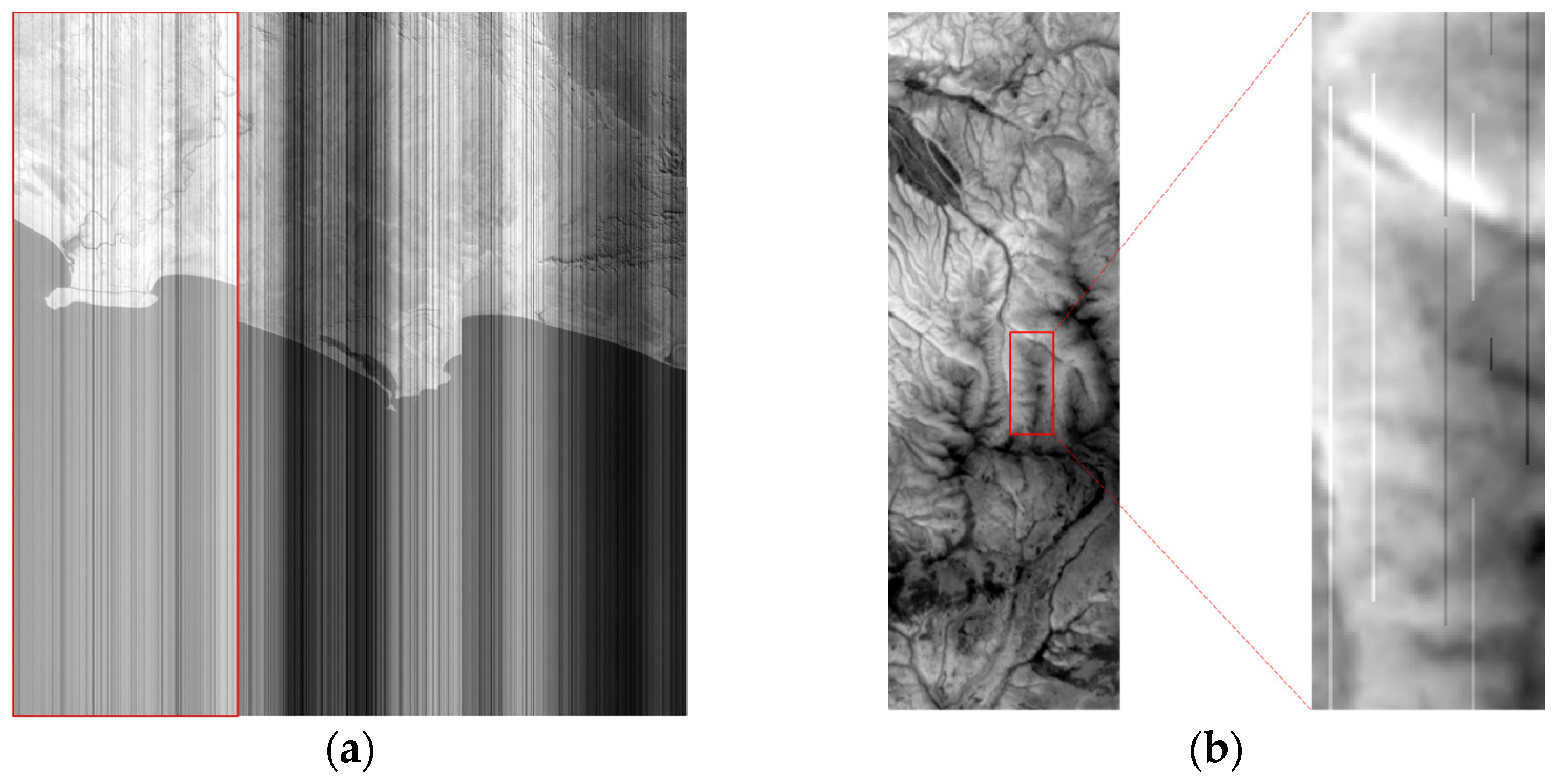
Band 9 (8.01~8.39 μm) and band 10 (8.42~8.83 μm) level 0 (L0) images that possess abundant stripe noise obtained from the VIMI sensor on the GF5-02 satellite are used to validate the effectiveness of the proposed trend repair method. Further information on the VIMI and GF5-02 satellites can be found in [30,31]. Notably, the VIMI utilizes a three-panel mosaic assembly technique to capture images with a swath width of 60 km at a spatial resolution of 40 m, which introduces discernible differences between neighboring sections. The focus of this paper is on testing a new method for removing stripe noise rather than addressing interplane calibration issues; therefore, a specific array that can easily distinguish stripe noise and is convenient for conducting experimentation among the three splicing planes is selected—covering a region of 1536 × 512 pixels on the leftmost side of the image, as exhibited within the red box in Figure 1a. Ten different GF5-02 VIMI scenes were analyzed, which contain different surface types, to verify the universality of the new method proposed in this paper. These scenes are displayed in Figure 2, and their detailed information is organized in Table 1.
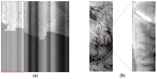
Figure 1.
Original thermal images of GF5-02 VIMI and Landsat 8 TIRS. (a) Image of GF5-02 VIMI band 9; (b) image of Landsat TIRS band 10 experimental area and the simulated stripe noises.
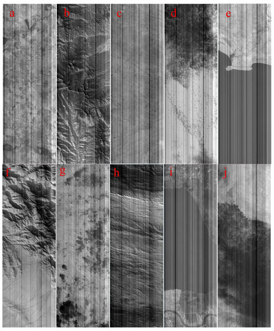
Figure 2.
GF5-02 VIMI experimental data including different surface types (one of three splicing panels in each image covers 1536 × 512 pixels, (a–j) are the numbers of these experimental images.).

Table 1.
Detailed information of GF5-02 VIMI images utilized in the experiment.
2.2. Landsat 8 TIRS Data
Landsat 8 band 10 (10.60~11.19 μm) L1 image data acquired on 26 October 2021 by TIRS at (37.09°N, 104.78°W) is used to verify the accuracy of the proposed trend repair method by simulating nonlinear stripe noise in advance. Considering the large swath width of the Landsat 8 band 10 image, this article crops the same size (1536 × 512 pixels) as the experimental area of the GF5-02 VIMI band 9 and band 10 images. The selected experimental area of the Landsat 8 TIRS band 10 image is displayed in Figure 1b, where the specific details within the red boxes of the simulated results are enlarged for enhanced visibility. This paper employs the Mersenne twister [32] engine and uniform int distribution in C++ in conjunction to simulate stripe noise to ascertain the sequence number of random simulated columns, as well as the random starting and ending positions of the stripe noise. Additionally, the degree of contamination in each selected column’s stripe noise region is generated using the Mersenne twister engine and uniform real distribution in C++ within the range of 0~10% relative to the mean value of the raw pixels in the randomly selected stripe area. Then, ten simulated images corresponding to contamination levels (0,0.01], (0.01,0.02], (0.02,0.03], (0.03,0.04], (0.04,0.05], (0.05,0.06], (0.06,0.07], (0.07,0.08], (0.08,0.09], (0.09,0.10] (0~1%, 1~2%, 2~3%, 3~4%, 4~5%, 5~6%, 6~7%, 7~8%, 8~9%, 9~10%) are produced with a total of 25 stripe noise columns on each image.
3. Methodology
The histogram matching method is one of the most representative techniques in the statistical category for addressing common stripe noises. In addition to removing common stripe noise effectively, it is particularly effective in mitigating nonlinear noise prevalent in sensor columns, even though the complete elimination of such noise may not be achieved [33]. Therefore, an innovative trend repair method that combines the strengths of the histogram matching method is proposed, providing a comprehensive solution to the challenges posed by both common and nonlinear stripe noise. Streaking, SSIM, PSNR, and IF are used to assess the variations in image uniformity, structure, and information before and after image correction.
3.1. Histogram Matching Method
The histogram matching method operates based on the fundamental assumption that all sensor detectors should exhibit a consistent response range in the same response function. It relies on the premise that when the image extent and pixel count are sufficiently large, the frequency histogram depicting the occurrence of various pixel values should demonstrate comparable profiles between each detector column and the entire image. Based on this hypothesis, the histogram matching algorithm constructs each column and the entire image cumulative probability density function (CPDF) separately. Then, a lookup table is built by matching different column CPDF curves to the entire image CPDF curve to correct the noisy satellite image. References [16,18,27] provide a more detailed explanation for a more comprehensive understanding of the histogram matching algorithm. Some of the key steps are briefly described below:
- (1)
- Calculate the probability density function (PDF) of each column and the entire image:
- (2)
- Calculate the CPDF of each PDF histogram:
- (3)
- Match each column CPDF curve to the entire image CPDF curve to obtain a lookup table:
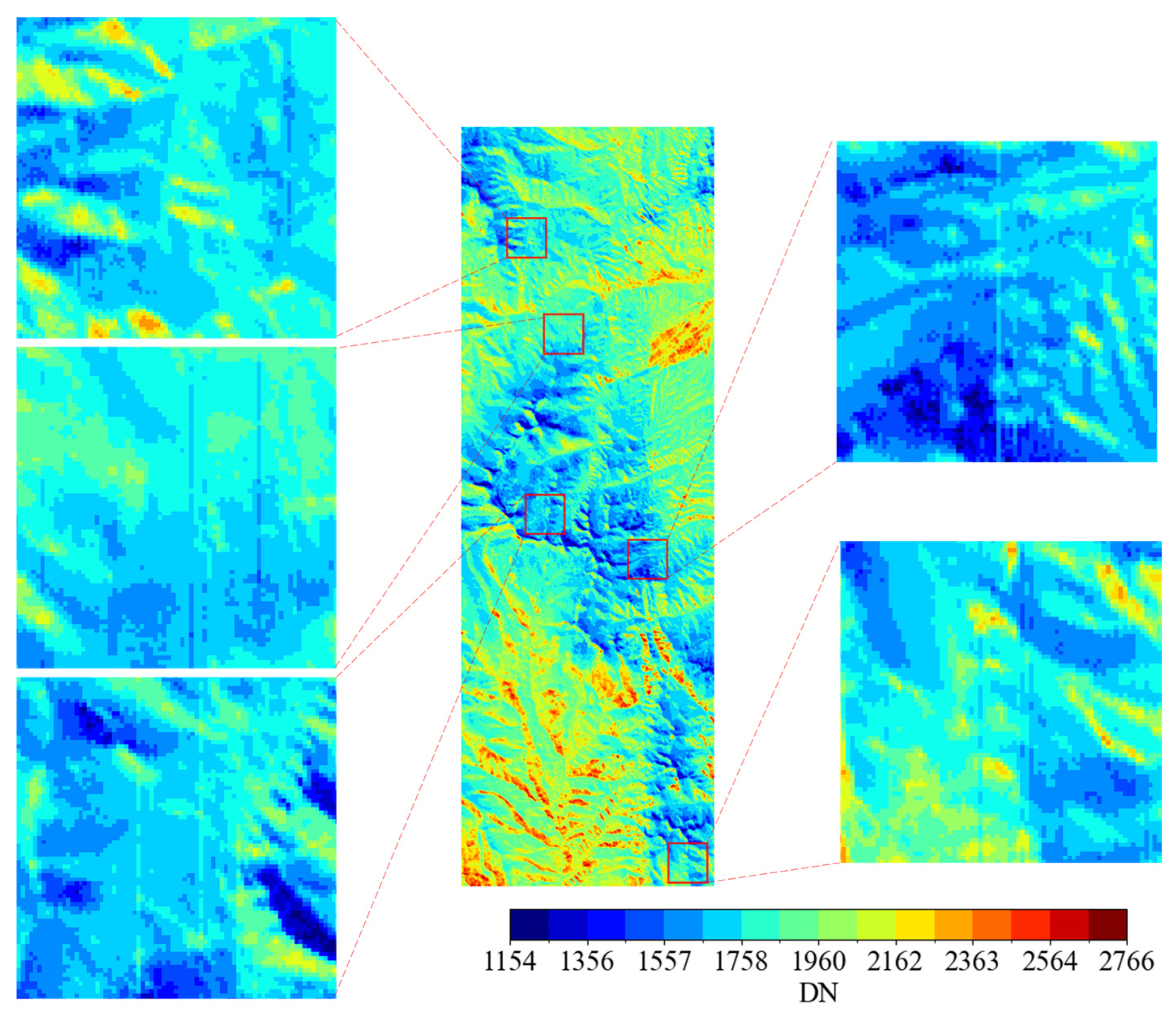
Figure 3 displays an enlarged view of the processed image b after histogram matching in Figure 2 and highlights nonlinear stripe noise with a pseudo-color transformation. Apparently, the histogram matching algorithm leaves certain nonlinear striping noises, which manifest as noncontinuous disruptions in columns and exhibit distinct gray levels compared to the surrounding pixels in the visual representation. Columns that contain this stripe noise are called defective columns, while other columns without this stripe noise are normal columns. The defective columns in the experimental images are picked out by visual interpretation in this paper. Addressing these defective columns is very important for the subsequent application of images.
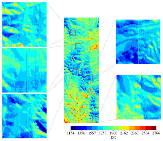
Figure 3.
Details of the nonlinear stripe noise on GF5-02 VIMI band 9.
3.2. Trend Repair Method
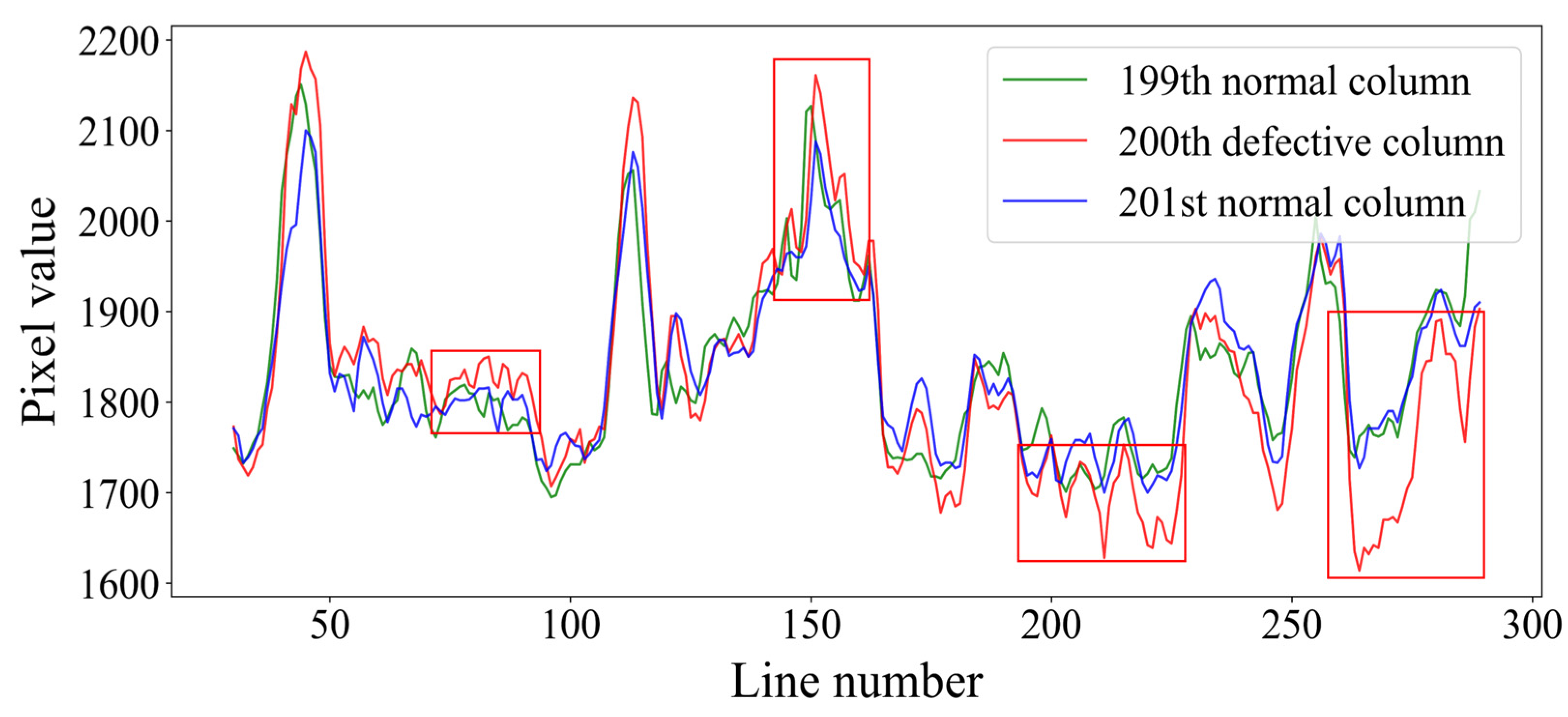
Comparing the defective column and the adjacent normal columns of image b in Figure 4 shows that the noisy regions in the red boxes within the defective column generally exhibit similar trends to the corresponding areas in the adjacent normal columns. Based on this observation, the nonlinear stripe noises that persist after applying the histogram matching algorithm are likely a result of the unstable operation of the detector over a certain period. This instability causes the base value (the mean of a certain segment within the column) to deviate from the normal level, resulting in nonlinear stripe noise. The key to eliminate this residual nonlinear stripe noise lies in accurately rectifying the base value of certain defective segments where the inner pixel values are different from other pixel values around it.
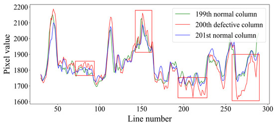
Figure 4.
Trend profiles of the defective column and normal columns in Figure 3. The red line is a part of the region of the 200th defective column, and the green and blue lines are a part of the region of the 199th and the 201st normal column, respectively. The red boxes indicate the noisy regions that the pixel values in the defective column deviate surrounding normal pixel values severely.
In fact, the images acquired from space by sensors are the records of actual conditions on the ground that possess geographical traits. Hence, according to the first law of geography [34], near objects have more similarities than distant objects. This is also appropriate to pixels on an image: near pixels have more similar statistical characteristics than distant pixels. This law provides a probability of using near-normal pixel values to correct abnormal pixel values. Meanwhile, for an abnormal pixel, its value contains not only the true value of a surface object but also noise. It is vital to keep more useful information by removing noise precisely.
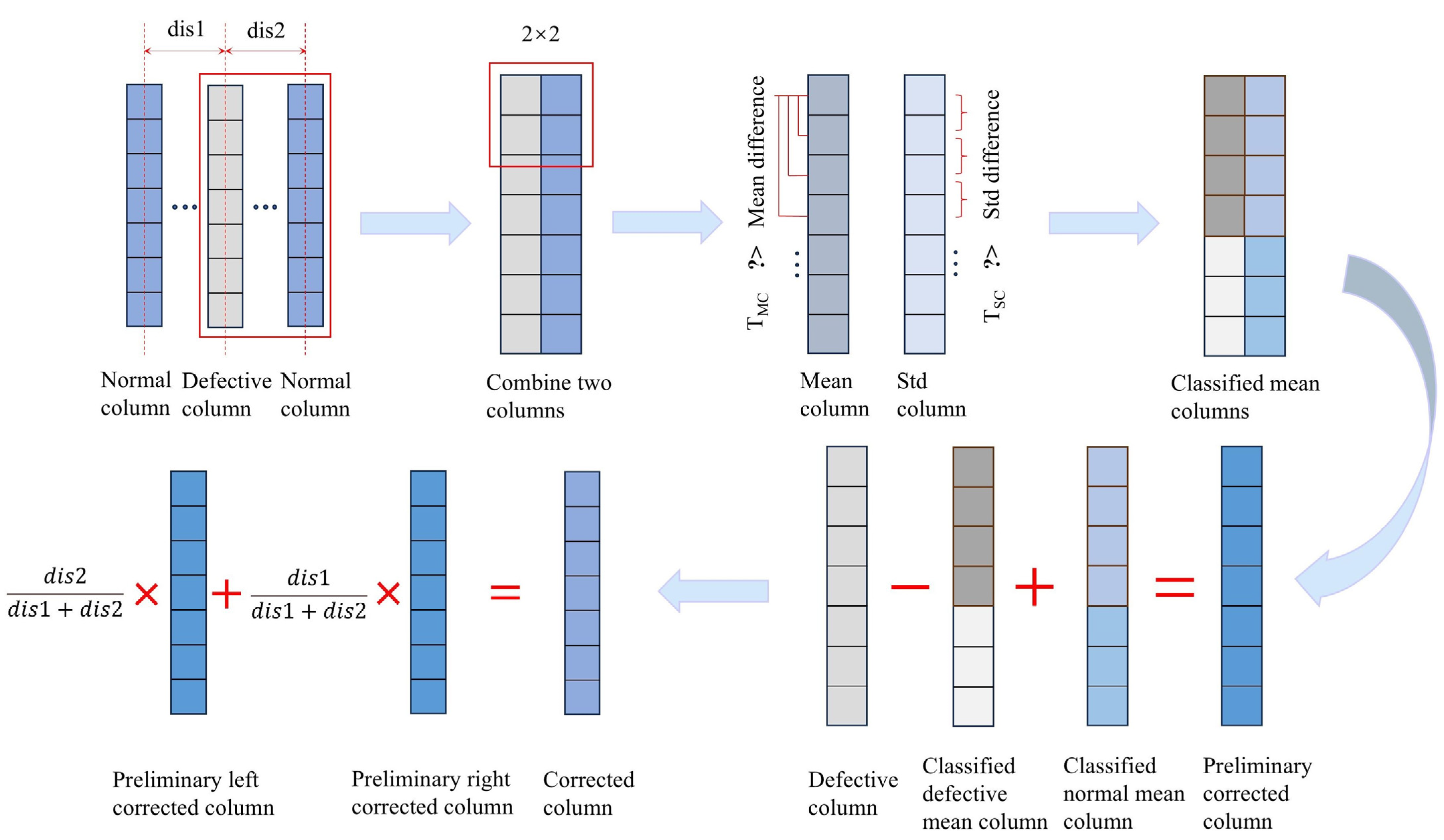
Therefore, this paper replaces the base value of the defective column with the base value calculated by the two adjacent normal columns in the same segment according to the hypothesis above to keep as much useful information as possible, creating an innovative trend repair method to recover the normal trends of the contaminated regions within the defective columns. Figure 5 depicts the entire processing flow, and the following steps were undertaken to implement the approach:
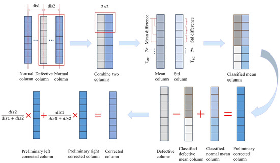
Figure 5.
Processing flow of the trend repair method (the Mean difference is the difference between the specific mean value and the value in the mean column. The Std difference represents the difference between two contiguous standard deviation values in the std column).
- (1)
- Find two nearest adjacent normal columns: find two adjacent normal columns located on both sides of the defective column; record the distances (dis1 and dis2) to the defective column separately.
- (2)
- Calculate the mean and standard deviation columns: combine one of two adjacent normal columns with the defective column and define a 2 × 2 window. Slide the window and calculate its mean and standard deviation iteratively. The mean column (MC) and standard deviation column (SC) are obtained at the end of the ergodic.
- (3)
- Classify within two columns: contrast the first mean value in the mean column with the subsequent mean values and compare each pair of contiguous standard deviation values in the standard deviation column acquired from previous steps in sequence. If the difference values are less than the preset thresholds TMC and TSC (these two thresholds are automatically determined according to the mean and standard deviation columns; for the calculation method, refer to Formulas (6) and (7)) simultaneously, then label the corresponding 2 × 2 pixels in the same class; otherwise, two pixels at the end of the current window are labeled as the beginning of another class. Then, the comparison steps are repeated until the final pixel is reached. Ultimately, the two combined columns are partitioned into several distinct segments, and corresponding segments which represent class in defective column (CDC) and class in normal column (CNC) exhibit similar structural characteristics.where and are thresholds to subsection. and are the mth values in mean and standard deviation columns acquired in step (2), respectively. is the mean value of the mean column, and is the length of the standard deviation column.
- (4)
- Calculate mean value: calculate mean values of the different classes in the defective column and corresponding normal column to reach classified mean columns.where and denote the mth class mean at the location of the defective column and the normal column separately. and denote the pixel value at the location in the mth class of the defective column and the normal column, respectively. and denote the number of pixels in the mth class of the defective column and the normal column.
- (5)
- Repeat the steps: for the other adjacent normal column, repeat steps (2) to (4).
- (6)
- Correct preliminarily: traverse every pixel in the original defective column, subtract the mean of the class to which the pixel belongs in the classified defective mean column from its initial value. Then, add the difference value to its corresponding class mean in the classified normal mean column to obtain its preliminary correction value:where denotes the preliminary correction columns combined with the left and right normal columns. represents the DN value at the ith line and jth column on the image. , and denote the mean value at location , and of the defective column and its left and right normal column, respectively.
- (7)
- Weight the preliminary corrected values: considering the influence of the geospatial structure of adjacent pixels on the contaminated value, calculate the final corrected value by preliminary correction values of both side pixels using the inverse distance weighting method:where is the corrected value at the ith line and the jth column on the image. dis1 and dis2 indicate the distance from the normal column to the left and right defective column, respectively. denotes the preliminary correction value obtained from step (6).
- (8)
- Traverse the defective column: traverse and correct each pixel in the defective columns to reach the new corrected image.
3.3. Index of Assessment
3.3.1. Streaking Metrics
Streaking metrics employ the mean value in the current column and its immediate neighbors to estimate whether the stripe exists between detectors [35]. Lower streaking metrics represent more uniform images. Because of its insensitivity to feature type on the ground, it is selected to evaluate the performance of the proposed method using the following equation:
where is the mean value of the ith column and and are the mean values of both sides of the ith column.
3.3.2. Structural Similarity
The SSIM combines three aspects (luminance comparison, contrast comparison, and structure comparison) to measure the relative signal quality in two images [36]. Normally, the range of SSIM values is between 0 and 1; the higher the SSIM is, the more similar the two images are. SSIM is calculated by Formula (14):
where and denote the means of the original and corrected images, respectively. denotes the covariance of the original and corrected images. and denote the standard deviations of the original and corrected images, respectively. and are two tiny constant values added to avoid dividing by zero.
3.3.3. Peak Signal-to-Noise Ratio
The PSNR is converted by the mean squared error (MSE), which describes the level of error or distortion between the original image and the processed image [37]. A large PSNR represents higher image quality in retaining the information and vice versa. PSNR is defined by the following equations:
where and denote the number of lines and columns, respectively. and denote the pixel values at the mth line and the nth column in the original image and the corrected image, respectively. denotes the maximum value of the original image data type.
3.3.4. Improvement Factor
The IF, which is an index of image quality after destriping, first appeared in an article by Corsini et al. [38], evaluating the effect of destriping on MOS-B data in the band direction. A higher IF indicates better improvement. IF is computed by the following equations:
where , , and represent the mean pixel value of the jth column for the push-broom scanner in the original image, the de-striped image, and the image that recorded the true value of the object, respectively. Because of the lack of a perfect image, a low-pass filter is applied to the de-striped image to accomplish the assignment.
4. Results
4.1. Visual Analysis
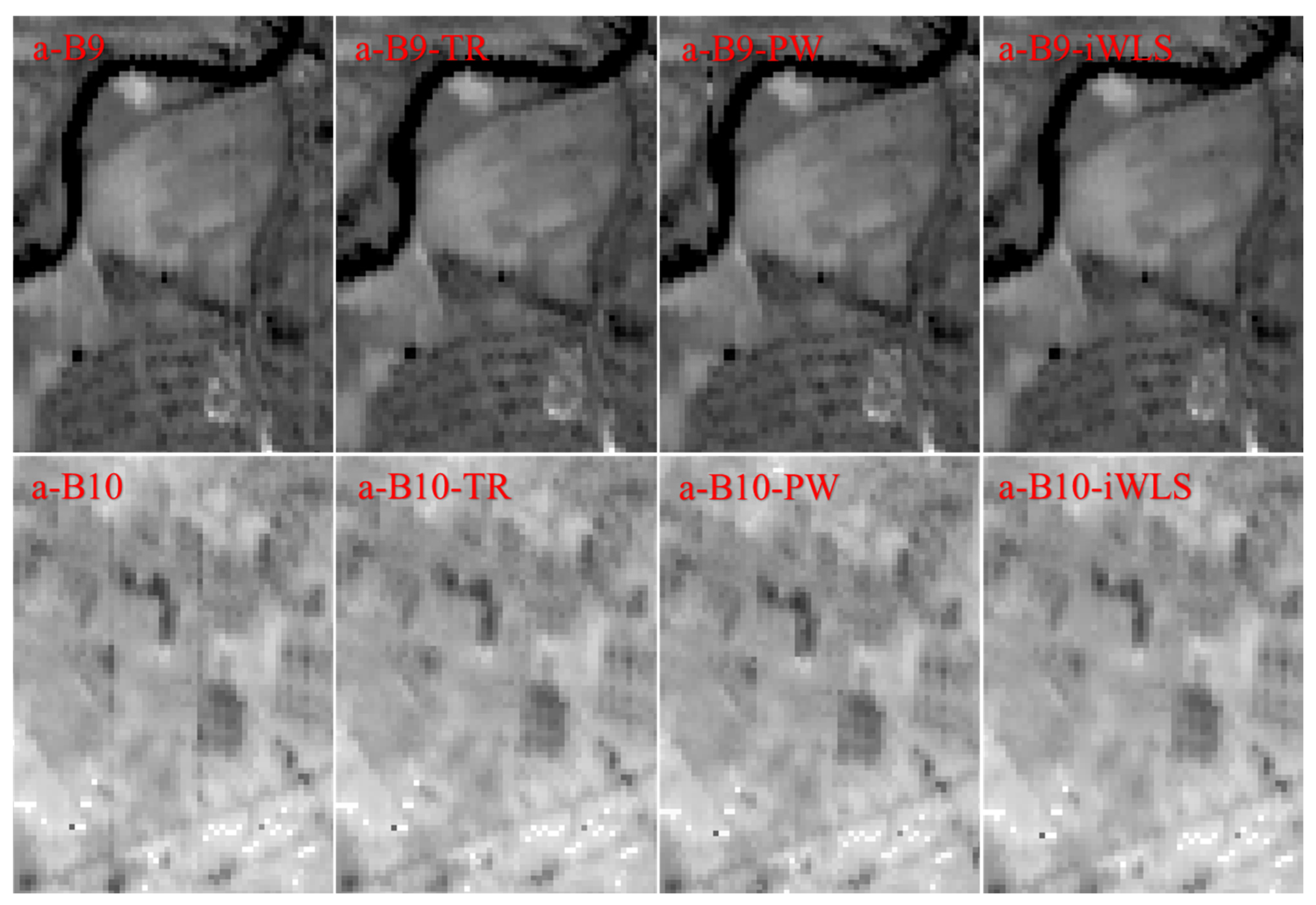
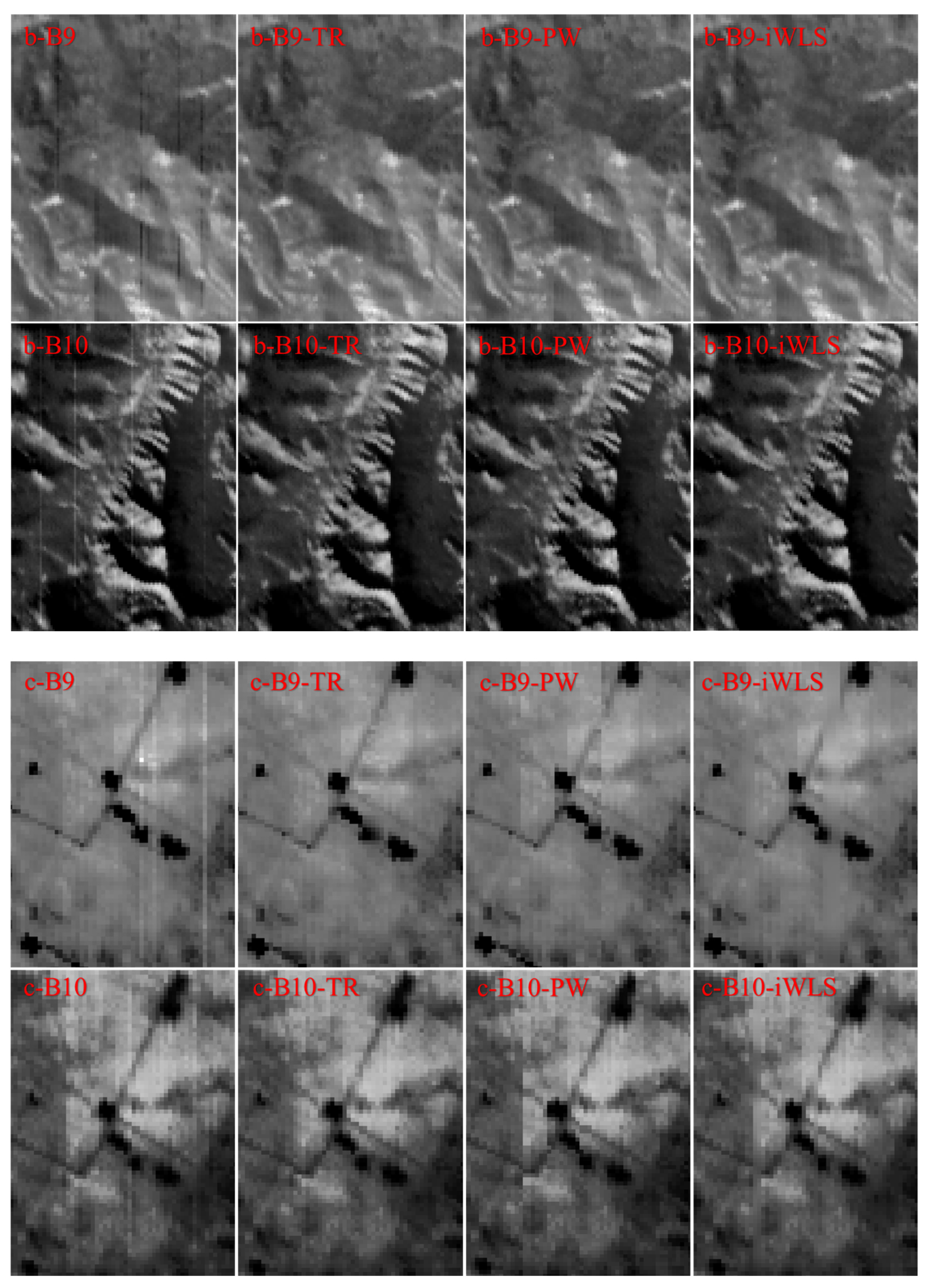
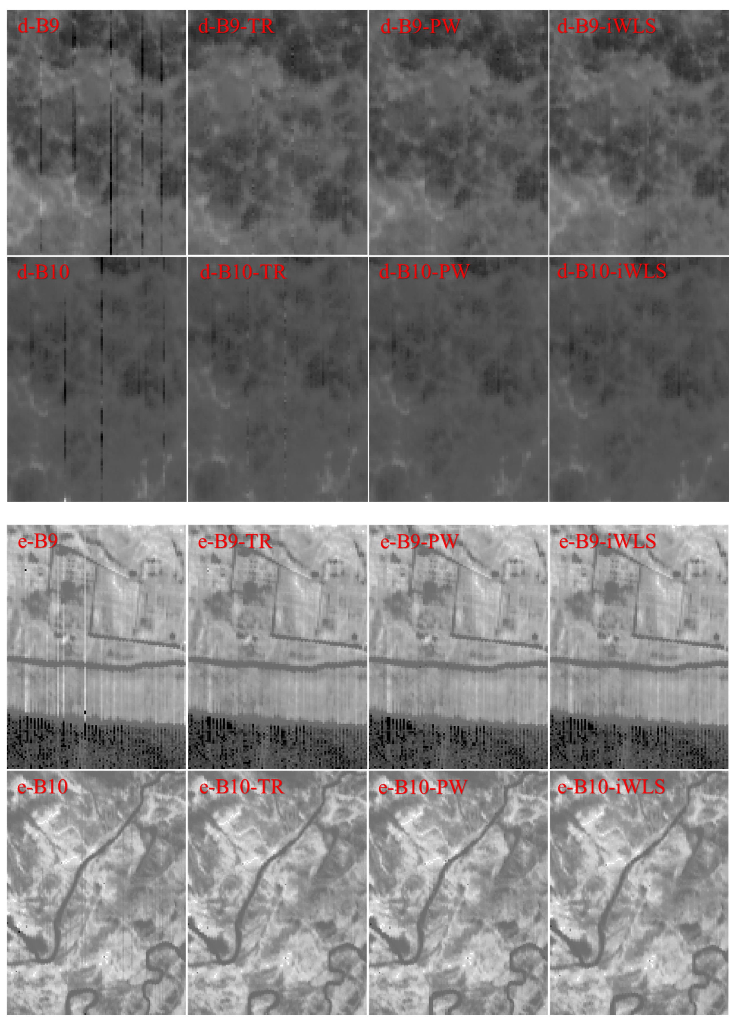
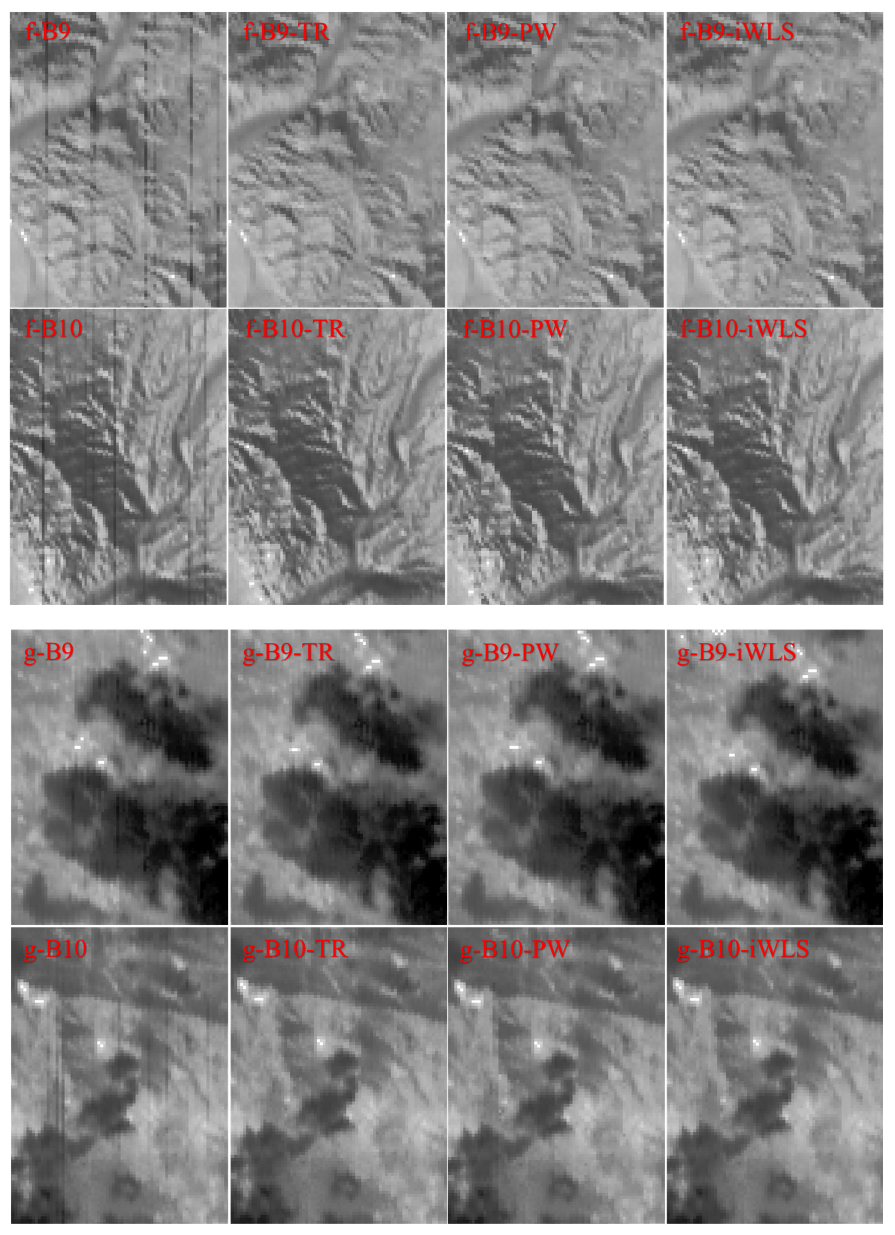
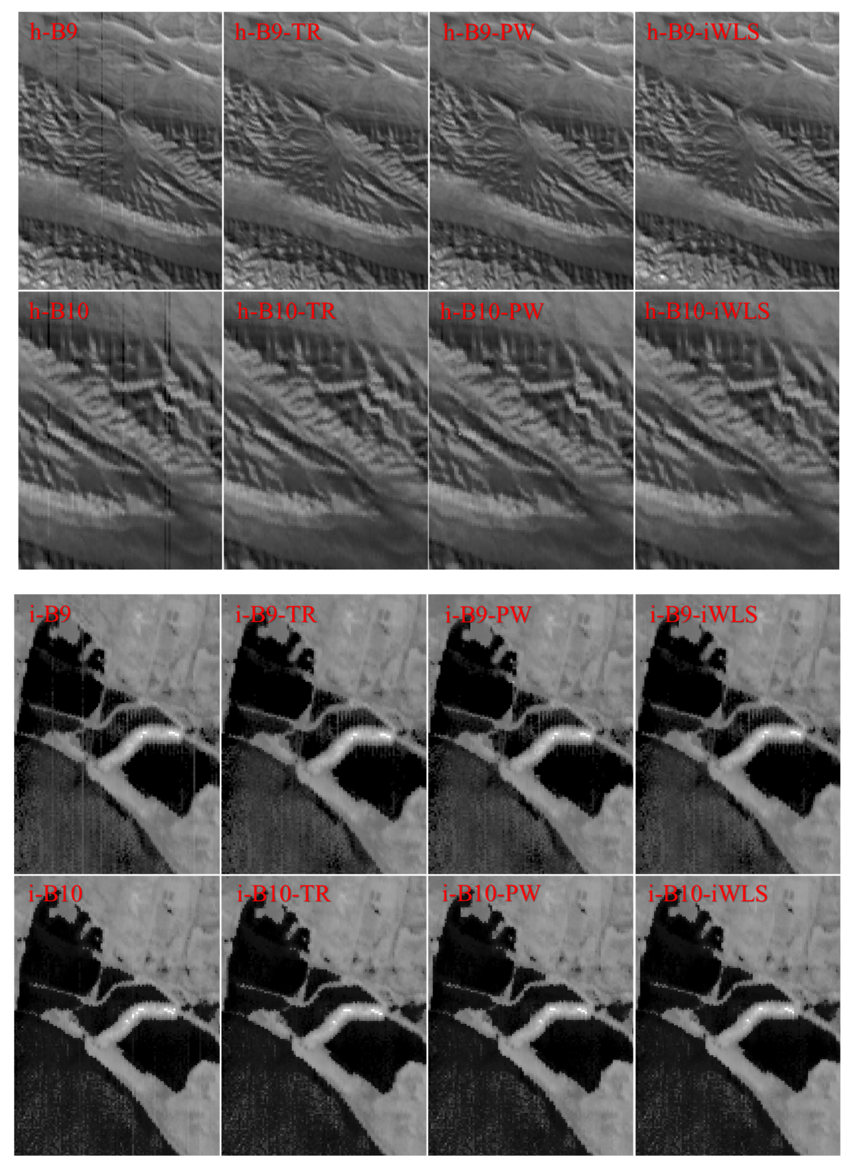
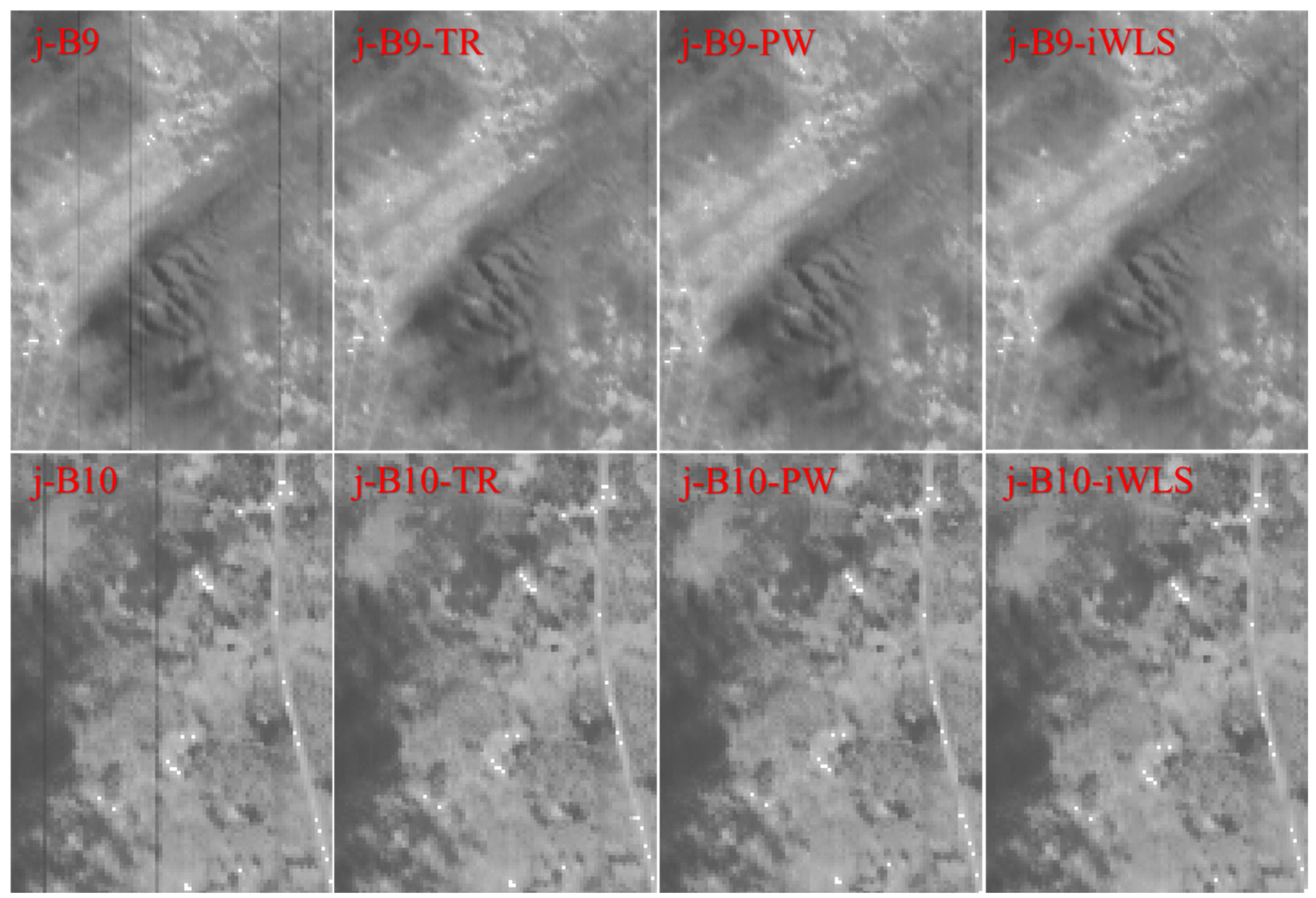
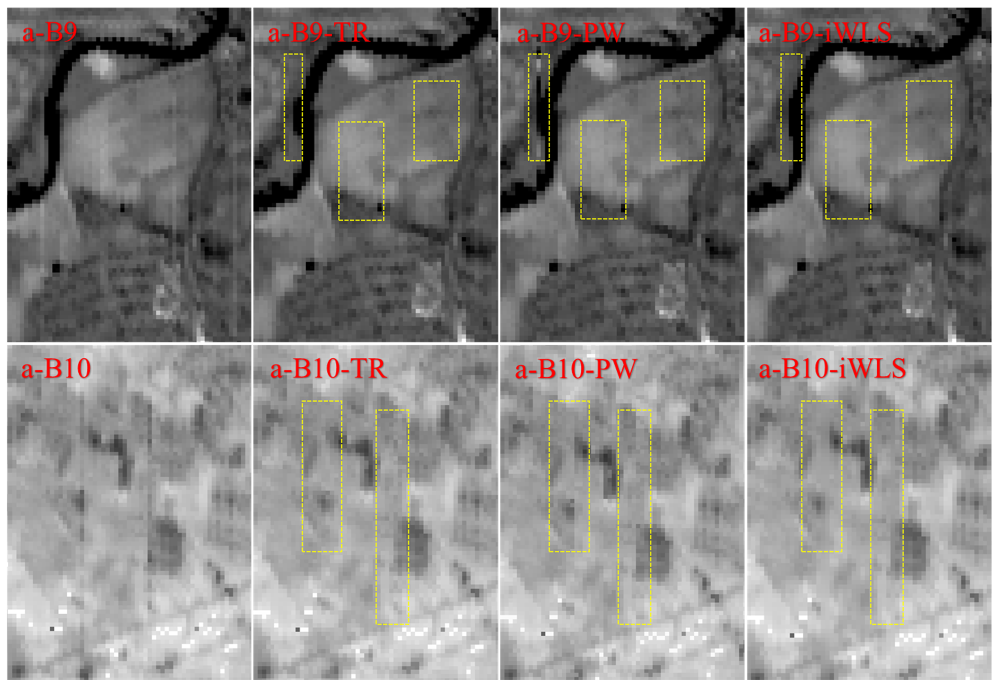
Figure 6 shows a set of partial images of bands 9 and 10 before and after using the trend repair method and the other two methods in the same area (other sets of results are displayed in Appendix A). Most stripe noise has been eliminated, and bands 9 and 10 of the image both become clear and similar to reality by applying the trend repair method. This means that the methods presented in this paper meet the requirements qualitatively. Furthermore, the characteristics of the three methods are implied according to more details in the yellow boxes in Figure 6, showing that the trend repair method corrects the image with a gradual process; restoration by the piece-wise method seems a little sudden, i.e., lacking the consideration of surrounding environments; and the iterated WLS method often smooths the stripe noise excessively. However, it is not sufficient to explain the specific strengths of the new method in a simple visual way. Therefore, a set of classical indices defined to evaluate image quality quantitatively in Section 2 is used hereafter. Two other published destriping methods are also compared with the trend repair method utilizing simulated Landsat 8 data in addition to GF5-02 VIMI data.
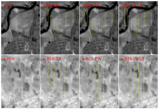
Figure 6.
Set of contrasting images of the GF5-02 VIMI bands 9 and 10 before and after using the trend repair method and the other two methods (a is the number of experimental images, B9 and B10 represent the histogram matching results on bands 9 and 10 of the GF-02 VIMI thermal bands, respectively. TR, PW and iWLS indicate the images corrected by the trend repair method, piece-wise method, and iterated WLS method, respectively. The yellow boxes highlight the differences between the three methods).
4.2. Results of the Assessment Index
This section employs Streaking, SSIM, PSNR, and IF as the key indices to assess the image variations in uniformity, structure, and information between images before and after correction to evaluate the effectiveness of the trend repair method quantitatively. Moreover, a comparative analysis of the trend repair method, juxtaposed against both the piece-wise method and the iterated WLS facet technique, is performed by processing identical GF5-02 VIMI experimental images, as previously described.
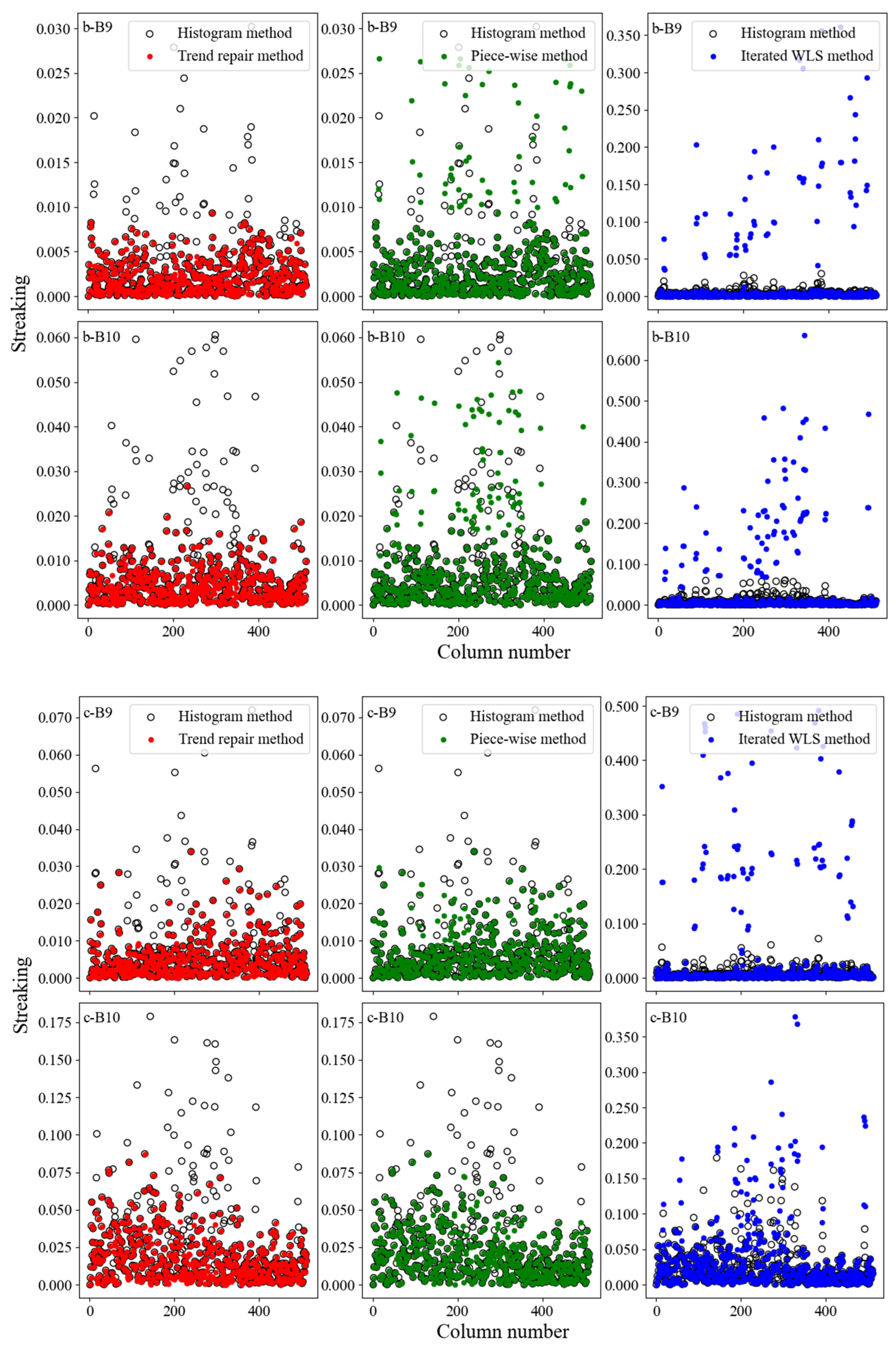
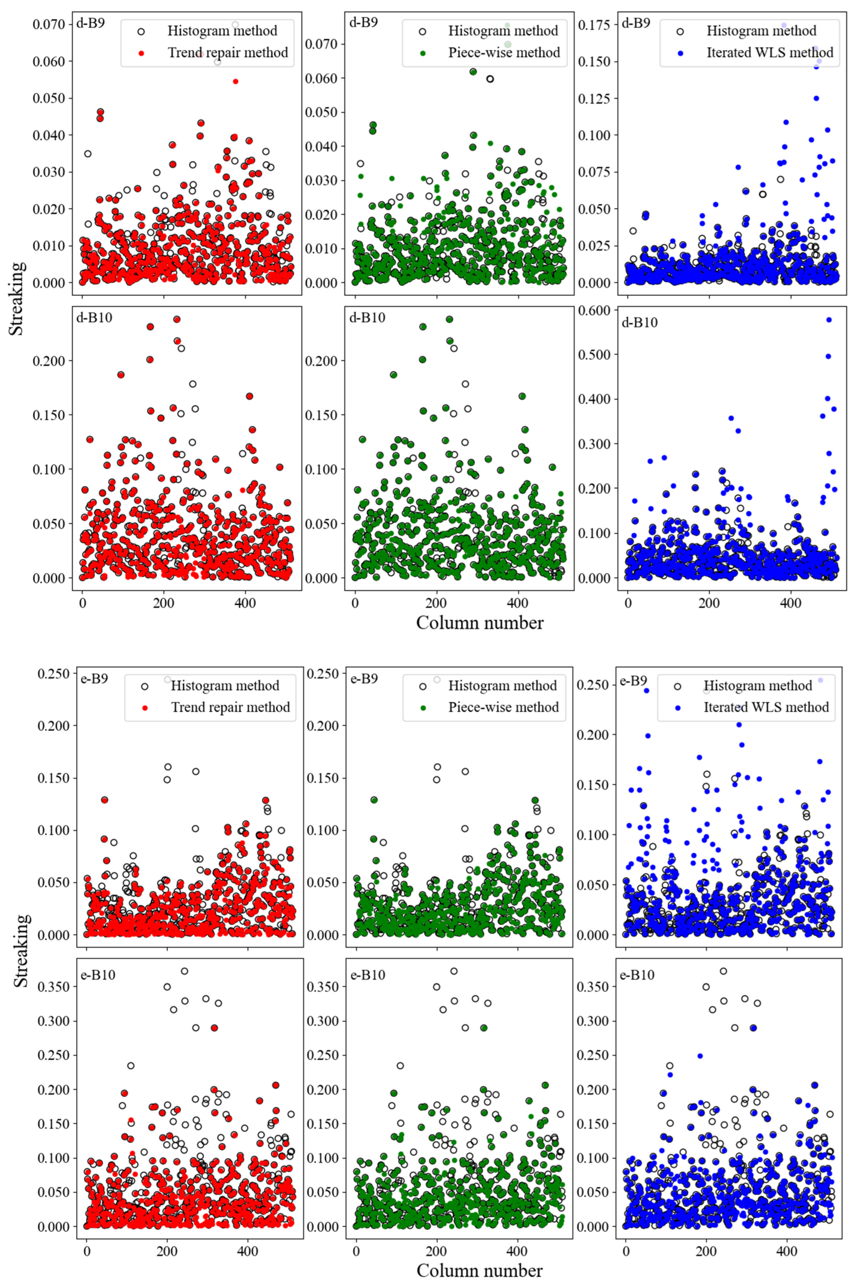
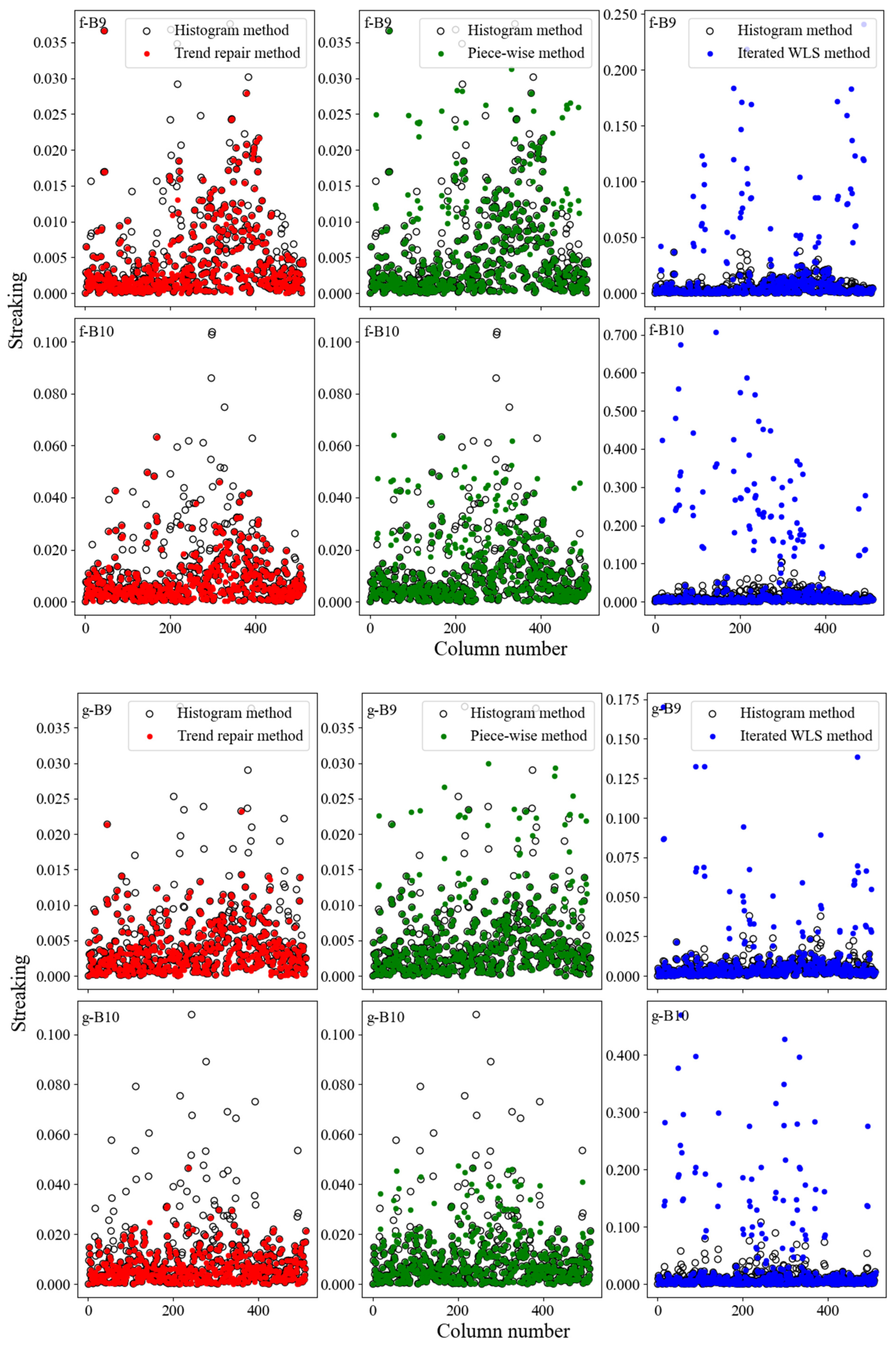
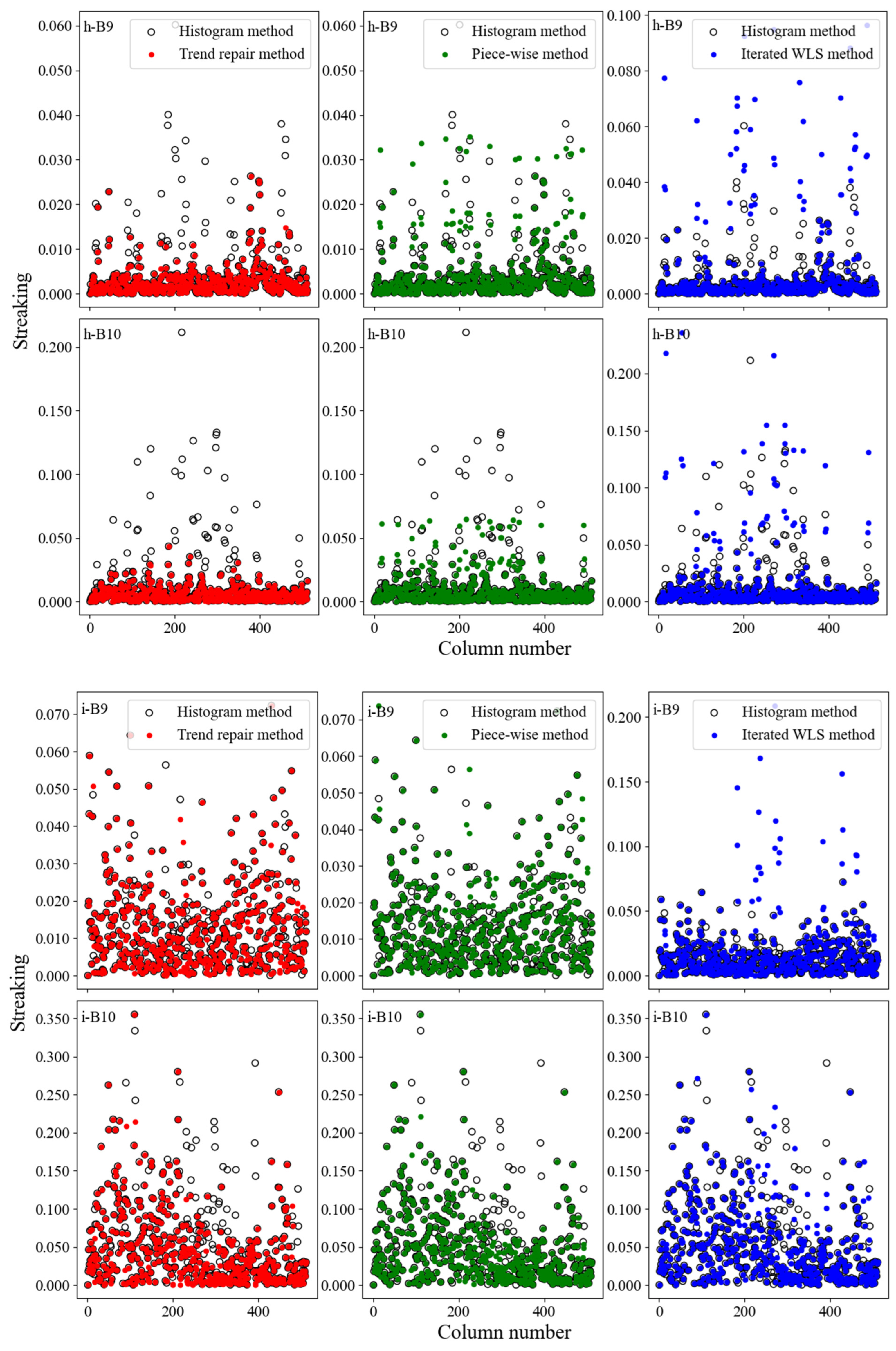
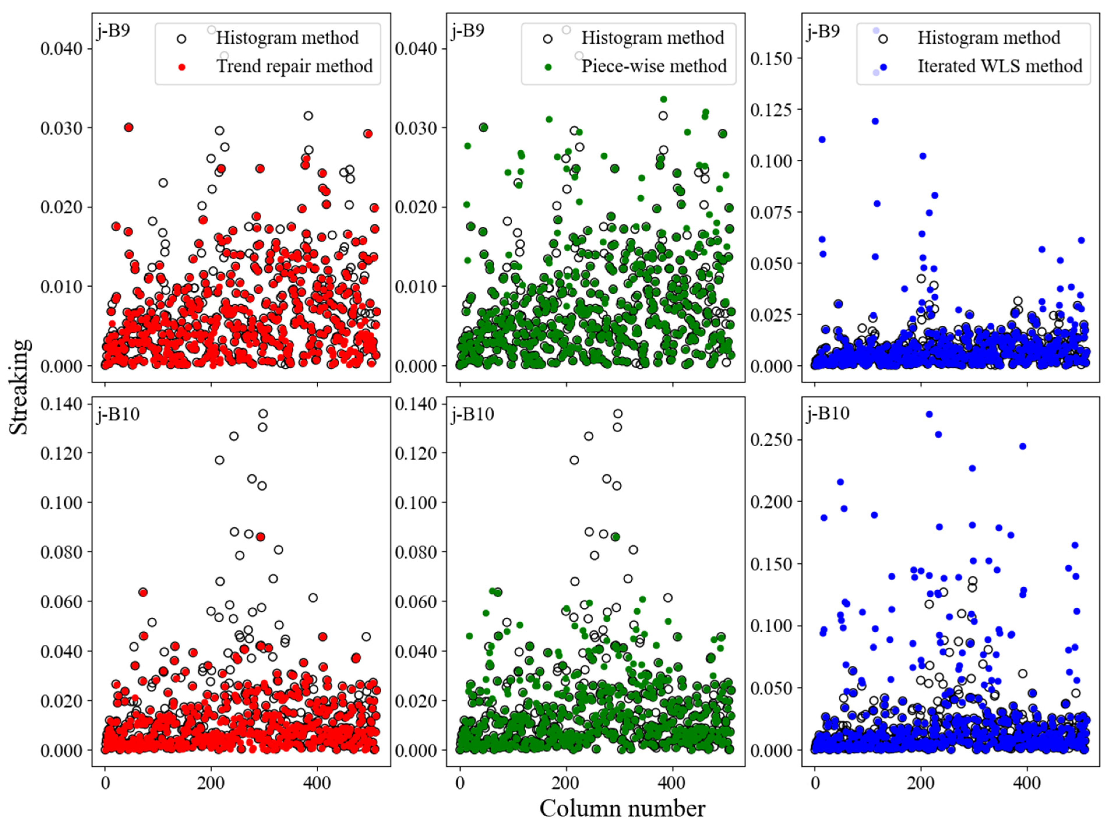
Figure 7 shows the Streaking scatterplot of each column on bands 9 and 10 of the GF5-02 VIMI experimental data (the results of other images are displayed in Appendix B). The hollow circle on the graph indicates the Streaking on the image without removing the stripe noise, while the solid dot represents the Streaking calculated on the image after the stripe noise is removed for specific columns. The hollow circles and the solid dots will coincide for normal columns that do not need to use the repairing method. Figure 7 shows that the columns that experienced the trend repair method became more consistent with the surrounding environment than the other two methods, as shown by a decrease in the value of the red dot.

Figure 7.
Comparison of the Streaking indices obtained using the trend repair method, the piece-wise method, and the iterated WLS method on bands 9 and 10 (B9 and B10) of the experimental image a.
The SSIM, PSNR, and IF calculation processes compare the statistical characteristics of the images before and after processing to determine whether the approach is valuable. Generally, these indicators use the whole image. In this experiment, however, the destriping method is not performed across the entire image, and the number of columns requiring correction is a small fraction of the total columns (approximately 1/20). Consequently, only the columns requiring correction were selected for computation, aiming to mitigate insignificant discrepancies in the results caused by normal columns.
The SSIM, PSNR, and IF results of the three methods in Table 2 indicate that the trend repair method provides more information and exhibits a greater degree of structural similarity to the original image than do the piece-wise method and the iterated WLS facet method in most cases. Especially notable is the IF indicator, whose value significantly surpasses those of the other two methods, which indicates a clear improvement in stripe removal effectiveness with the trend repair method. We also observed that the results on image d show that the SSIM and PSNR of the iterated WLS facet method slightly outperform those of the new method in this paper. This is probably because the clouds on the d image exhibit rapid numerical variations, resulting in many instances of single-pixel segments during the segmentation process. These single-pixel segments often represent extreme or outlier points, leading to significant changes in the structural integrity and information content of the corrected columns compared to the original columns in some areas (more details can be seen from the results on image d in Appendix A). However, the new method still results in a more pronounced elimination of stripe noise when considering the IF indicator, which characterizes the status of stripe removal.
Table 2.
Comparison of three methods assessed by three indices.
As described above, a conclusion can be drawn that the trend repair method effectively removes stripe noise while ensuring the maximal preservation of image structure and information content, possessing a comparative advantage over other methods.
4.3. Accuracy
Although the indices above evaluate the image quality before and after correction quantitatively, these indicators still cannot clarify how much bias compared to the real value will be achieved by employing the proposed trend repair method in this paper. Hence, a simulated stripe noise image from Landsat 8 band 10 introduced in Section 2 was used to evaluate the rectified accuracy of the method. Afterward, the stability of these three methods on different degrees of stripe noise contamination is also explored in this section.
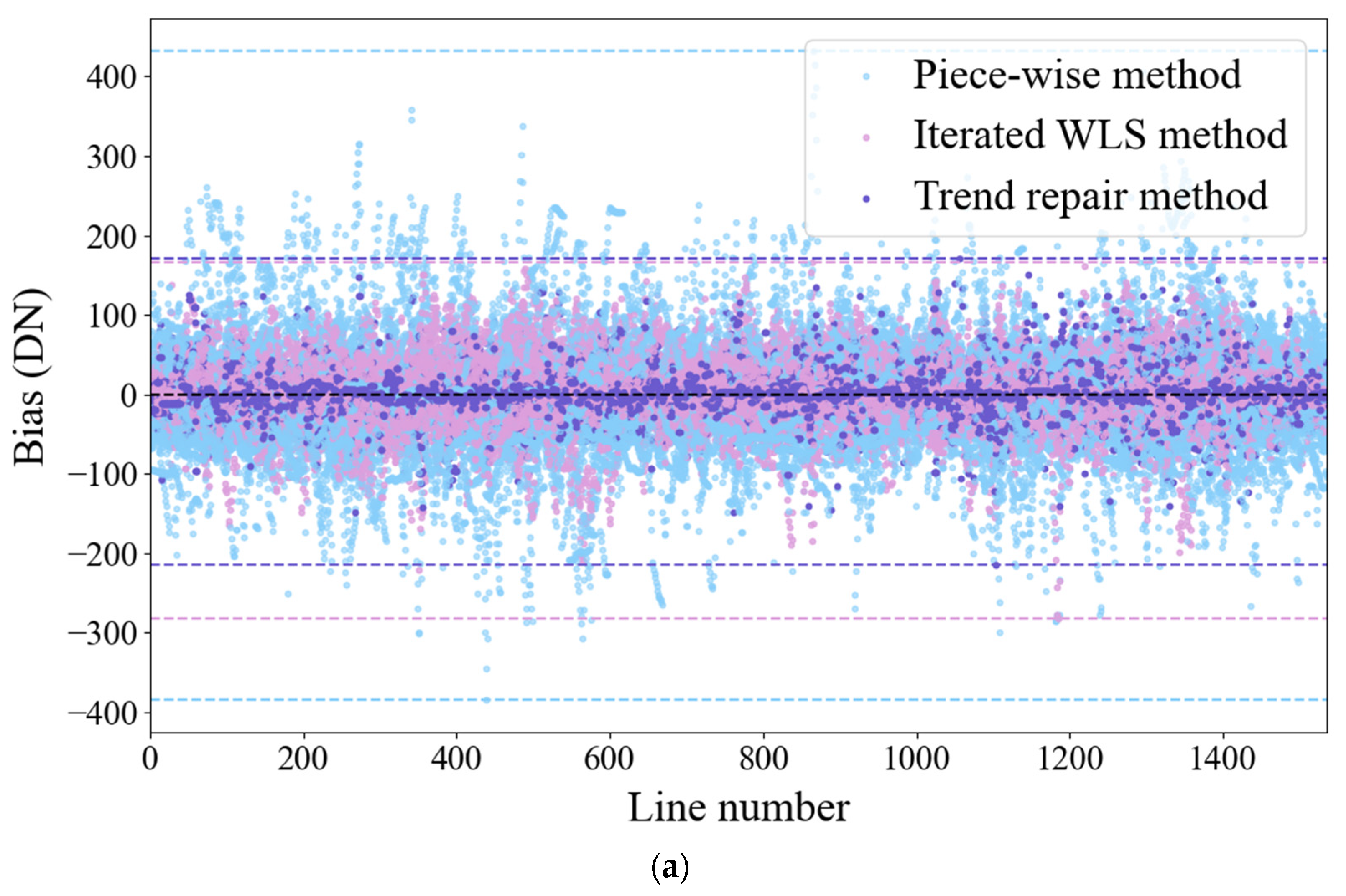
Figure 8a displays the bias between the corrected images obtained through the three methods individually and the original simulated image with a 1% degree of contamination. The image corrected by the proposed trend repair method causes smaller errors, with the majority of biases fluctuating around the zero line within the range of −214 to ~174, with a standard deviation of 18.36. Nevertheless, the bias introduced by the iterated WLS method spans the range of −282 to ~166, while the piece-wise method leads to significant errors within the range of −385 to ~432, with standard deviations of 31.97 and 59.61, respectively. Notably, the fluctuation range in the case of the piece-wise method is nearly twice that observed in the trend repair method. The maximum bias of the proposed trend repair method results in an error of approximately 1.10% relative to the mean of the entire original Landsat 8 band 10 experimental area. In comparison, it is approximately 1.44% of the iterated WLS method and 2.21% of the piece-wise method equivalent to 0.62 K, 0.82 K, and 1.25 K, respectively, when converted to the temperature according to the formula provided in the official documentation [39].

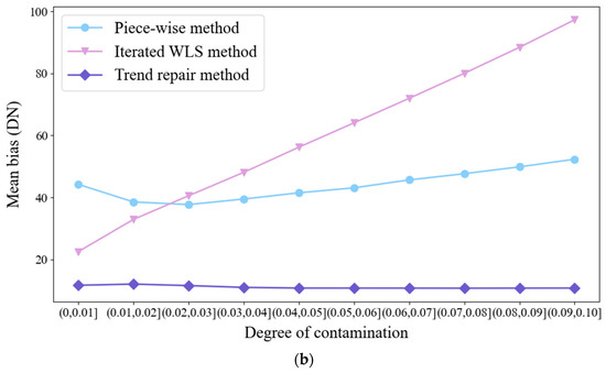
Figure 8.
Bias between the corrected image and the original image of the simulated Landsat 8 band 10 experimental data. (a) Bias after implementing three methods on the simulated image of 0~1% degree contamination; (b) Variation in average bias between different corrected contaminating images.
Additionally, Figure 8b shows that as the level of contamination increases, the deviations of the other two methods also show varying degrees of increase. Specifically, the correction deviation of the iterated WLS method increases rapidly. In contrast, the trend repair method demonstrates relatively stable performance, and the average bias consistently remains below 15 DN; moreover, its effectiveness improves with higher contamination levels. The underlying cause of this phenomenon is that as the contamination level increases, the stripe noise boundaries become more pronounced, making segmentation in step (3) more rational.
Hence, the trend repair method proposed in this paper has a credible ability to correct the nonlinear and random stripe noise in thermal band images.
5. Conclusions and Discussion
Common and nonlinear stripe noise are two kinds of stripe noise in the original remote sensing L0 images. The representative statistical histogram matching method is validated to be feasible for removing common stripe noise. This paper proposes an innovative method named the trend repair method to remove residual stripe noise based on rectifying the trend in the defective column with the adjacent normal columns’ mean value to correct the nonlinear stripe noise after histogram matching on the original remote sensing image data. Then, the results are compared with those of the piece-wise method and the iterated WLS method by processing the same image data containing a variety of surface types. The experimental results showed that the method proposed in this paper attains a better effect both visually and quantitatively by retaining maximal spatial structures and information content. It demonstrates superior performance in terms of the rectified accuracy and the stability of stripe noise removal across different contamination levels.
The trend repair method improves the original image quality after histogram matching by considering the geospatial structure. Compared to the piece-wise method, which uses only a single column as a reference, and the iterated WLS facet filter method, which uses neighborhood information excessively, the new method is theoretically and practically more convincing. In addition, the trend repair method preserves the range of changes in the value relative to the average level well.
The thresholds of the mean and standard deviation columns are the keys to segmenting the pixels in the defective column and the adjacent pairs of normal columns, as they directly influence the precision of the rectified results. The more pixels are in the right segment, the better the peak will be preserved. Although the definitions of thresholds TMC and TSC are automatically determined in Section 3, in practical applications, the boundary pixels between the normal and contaminated regions may encounter misclassification issues, leading to significant deviations in the correction results. Furthermore, if the pixel values in the defective column vary dramatically, the extrema may be segmented improperly, and the efficiency of the method will be impaired, and new stripe noise may arise due to outliers. Therefore, determining thresholds or segmentation methods requires further exploration.
Whether this novel trend repair method is suitable for other satellites or sensors is not discussed in this paper. Moreover, this paper focuses on removing residual stripe noise after preliminary correction using the histogram matching method. Therefore, more investigations on eliminating nonlinear or random stripe noise before relative radiometric calibration of the entire image are necessary.
Author Contributions
Conceptualization, Y.D.; Methodology, Y.D. and Z.Z.; Software, Z.Z.; Validation, Z.Z. and G.Z.; Formal analysis, Y.C.; Investigation, G.Z.; Resources, Y.D. and H.L.; Data curation, H.L.; Writing—original draft preparation, Z.Z.; Writing—review and editing, Z.Z., H.L., Y.D., Z.B., B.C. and Y.C.; Supervision, Y.D. and H.L.; Project administration, H.L.; Funding acquisition, H.L., Q.L. and Q.X. All authors have read and agreed to the published version of the manuscript.
Funding
This research was funded by the Chinese Natural Science Foundation Project (41930111, 42471365, 42071317, 42271362 and 42130111).
Data Availability Statement
The GF5-02 VIMI and Landsat8 TIRS images used in this study can be accessed at the China Centre for Resources Satellite Data and Application and GloVis, respectively.
Conflicts of Interest
The authors declare no conflicts of interest.
Appendix A
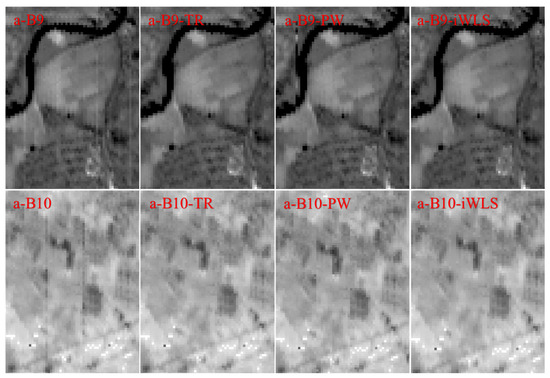
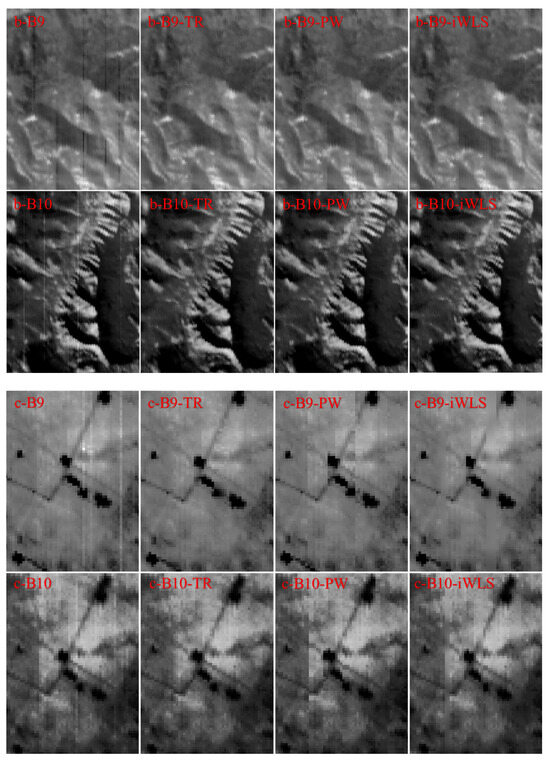
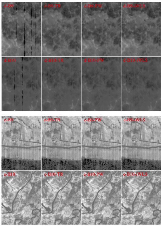
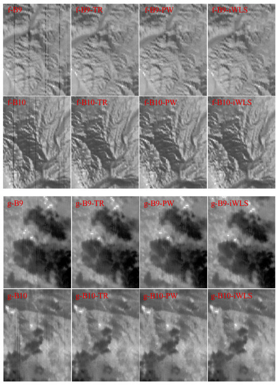
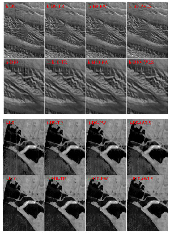
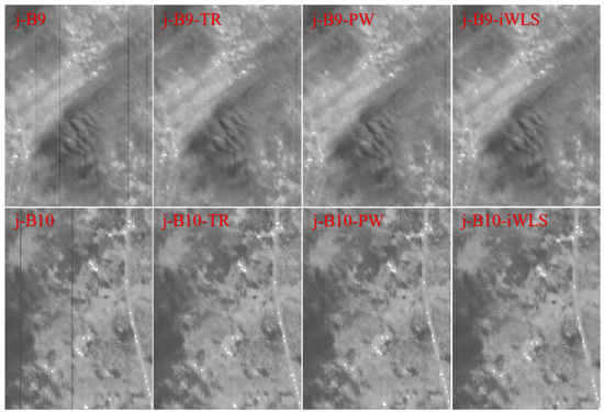
Figure A1.
Whole sets of experimental results of GF5-02 VIMI thermal band ((a–j) are the numbers of experimental images, B9 and B10 represent the histogram matching results on bands 9 and 10 of the GF-02 VIMI thermal bands, respectively. TR, PW, and iWLS indicate the images corrected by the trend repair method, piece-wise method, and iterated WLS method, respectively).
Appendix B
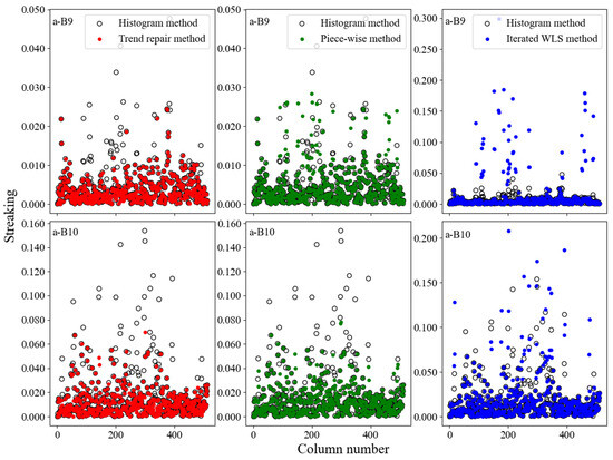

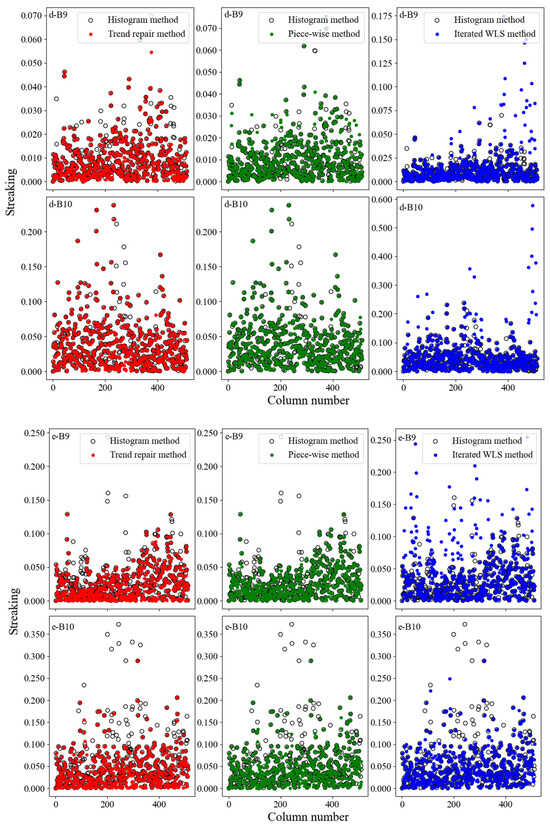
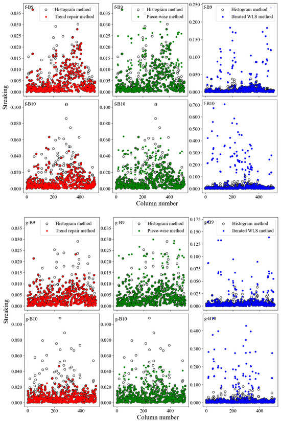

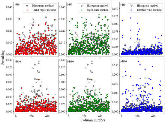
Figure A2.
Whole sets of Streaking results of GF5-02 VIMI thermal band ((a–j)are the numbers of experimental images, B9 and B10 represent the histogram matching results on bands 9 and 10 of the GF-02 VIMI thermal bands, respectively.
Figure A2.
Whole sets of Streaking results of GF5-02 VIMI thermal band ((a–j)are the numbers of experimental images, B9 and B10 represent the histogram matching results on bands 9 and 10 of the GF-02 VIMI thermal bands, respectively.

References
- Liu, J.G. Remote Sensing | Passive Sensors. In Reference Module in Earth Systems and Environmental Sciences; Elsevier: Amsterdam, The Netherlands, 2013; p. 9780124095489029560. ISBN 978-0-12-409548-9. [Google Scholar]
- Yan, F.; Wu, S.; Zhang, Q.; Liu, Y.; Sun, H. Destriping of Remote Sensing Images by an Optimized Variational Model. Sensors 2023, 23, 7529. [Google Scholar] [CrossRef] [PubMed]
- Cao, B.; Du, Y.; Xu, D.; Li, H.; Liu, Q. An Improved Histogram Matching Algorithm for the Removal of Striping Noise in Optical Remote Sensing Imagery. Optik 2015, 126, 4723–4730. [Google Scholar] [CrossRef]
- Chen, B.; Liu, L.; Zou, Z.; Shi, Z. Target Detection in Hyperspectral Remote Sensing Image: Current Status and Challenges. Remote Sens. 2023, 15, 3223. [Google Scholar] [CrossRef]
- Li, R.; Li, H.; Hu, T.; Bian, Z.; Liu, F.; Cao, B.; Du, Y.; Sun, L.; Liu, Q. Land Surface Temperature Retrieval From Sentinel-3A SLSTR Data: Comparison Among Split-Window, Dual-Window, Three-Channel, and Dual-Angle Algorithms. IEEE Trans. Geosci. Remote Sens. 2023, 61, 5003114. [Google Scholar] [CrossRef]
- Li, H.; Li, R.; Yang, Y.; Cao, B.; Bian, Z.; Hu, T.; Du, Y.; Sun, L.; Liu, Q. Temperature-Based and Radiance-Based Validation of the Collection 6 MYD11 and MYD21 Land Surface Temperature Products Over Barren Surfaces in Northwestern China. IEEE Trans. Geosci. Remote Sens. 2021, 59, 1794–1807. [Google Scholar] [CrossRef]
- Bian, Z.; Roujean, J.L.; Fan, T.; Dong, Y.; Hu, T.; Cao, B.; Li, H.; Du, Y.; Xiao, Q.; Liu, Q. An Angular Normalization Method for Temperature Vegetation Dryness Index (TVDI) in Monitoring Agricultural Drought. Remote Sens. Environ. 2023, 284, 113330. [Google Scholar] [CrossRef]
- Freitas, S.C.; Trigo, I.F.; Bioucas-Dias, J.M.; Gottsche, F.-M. Quantifying the Uncertainty of Land Surface Temperature Retrievals From SEVIRI/Meteosat. IEEE Trans. Geosci. Remote Sens. 2010, 48, 523–534. [Google Scholar] [CrossRef]
- Zhao, X.; Li, M.; Nie, T.; Han, C.; Huang, L. An Innovative Approach for Removing Stripe Noise in Infrared Images. Sensors 2023, 23, 6786. [Google Scholar] [CrossRef]
- Srinivasan, R.; Cannon, M.; White, J. Landsat Data Destriping Using Power Spectral Filtering. Opt. Eng. 1988, 27, 939–943. [Google Scholar] [CrossRef]
- Green, A.A.; Berman, M.; Switzer, P.; Craig, M.D. A Transformation for Ordering Multispectral Data in Terms of Image Quality with Implications for Noise Removal. IEEE Trans. Geosci. Remote Sens. 1988, 26, 65–74. [Google Scholar] [CrossRef]
- Donoho, D.L. De-Noising by Soft-Thresholding. IEEE Trans. Inform. Theory 1995, 41, 613–627. [Google Scholar] [CrossRef]
- Chang, S.G.; Yu, B.; Vetterli, M. Adaptive Wavelet Thresholding for Image Denoising and Compression. IEEE Trans. Image Process. 2000, 9, 1532–1546. [Google Scholar] [CrossRef]
- Pande-Chhetri, R.; Abd-Elrahman, A. De-Striping Hyperspectral Imagery Using Wavelet Transform and Adaptive Frequency Domain Filtering. ISPRS J. Photogramm. Remote Sens. 2011, 66, 620–636. [Google Scholar] [CrossRef]
- Alaeiyan, H.; Mosavi, M.R.; Ayatollahi, A. Hybrid Noise Removal to Improve the Accuracy of Inertial Sensors Using Lifting Wavelet Transform Optimized by Genetic Algorithm. Alex. Eng. J. 2023, 80, 326–341. [Google Scholar] [CrossRef]
- Horn, B.K.P.; Woodham, R.J. Destriping LANDSAT MSS Images by Histogram Modification. Comput. Graph. Image Process. 1979, 10, 69–83. [Google Scholar] [CrossRef]
- Fischel, D. Validation of the Thematic Mapper Radiometric and Geometric Correction Algorithms. IEEE Trans. Geosci. Remote Sens. 1984, GE-22, 237–242. [Google Scholar] [CrossRef]
- Gadallah, F.L.; Csillag, F.; Smith, E.J.M. Destriping Multisensor Imagery with Moment Matching. Int. J. Remote Sens. 2000, 21, 2505–2511. [Google Scholar] [CrossRef]
- Li, M.; Nong, S.; Nie, T.; Han, C.; Huang, L.; Qu, L. A Novel Stripe Noise Removal Model for Infrared Images. Sensors 2022, 22, 2971. [Google Scholar] [CrossRef] [PubMed]
- Kuang, X.; Sui, X.; Chen, Q.; Gu, G. Single Infrared Image Stripe Noise Removal Using Deep Convolutional Networks. IEEE Photonics J. 2017, 9, 3900913. [Google Scholar] [CrossRef]
- Xiao, P.; Guo, Y.; Zhuang, P. Removing Stripe Noise from Infrared Cloud Images via Deep Convolutional Networks. IEEE Photonics J. 2018, 10, 7801114. [Google Scholar] [CrossRef]
- Weinreb, M.P.; Xie, R.; Lienesch, J.H.; Crosby, D.S. Destriping GOES Images by Matching Empirical Distribution Functions. Remote Sens. Environ. 1989, 29, 185–195. [Google Scholar] [CrossRef]
- Su, J.; Zhou, C.; Li, Y.; Zhang, K. Relative Radiometric Correction of OHS Remote Sensing Images Based on Improved Moment Matching. Geomat. Spat. Inf. Technol. 2021, 44, 98–101. [Google Scholar]
- Wang, H.; Yu, J.; Li, Z. Analysis of Relative Calibration Algorithm of Space-Borne Infrared Camera. Spacecr. Recovery Remote Sens. 2009, 30, 44–49. [Google Scholar]
- Pesta, F.; Bhatta, S.; Helder, D.; Mishra, N. Radiometric Non-Uniformity Characterization and Correction of Landsat 8 OLI Using Earth Imagery-Based Techniques. Remote Sens. 2015, 7, 430–446. [Google Scholar] [CrossRef]
- Li, L.; Zhang, G.; Jiang, Y.; Shen, X. An Improved On-Orbit Relative Radiometric Calibration Method for Agile High-Resolution Optical Remote-Sensing Satellites with Sensor Geometric Distortion. IEEE Trans. Geosci. Remote Sens. 2022, 60, 1–15. [Google Scholar] [CrossRef]
- Wegener, M. Destriping Multiple Sensor Imagery by Improved Histogram Matching. Int. J. Remote Sens. 1990, 11, 859–875. [Google Scholar] [CrossRef]
- Rakwatin, P.; Takeuchi, W.; Yasuoka, Y. Stripe Noise Reduction in MODIS Data by Combining Histogram Matching with Facet Filter. IEEE Trans. Geosci. Remote Sens. 2007, 45, 1844–1856. [Google Scholar] [CrossRef]
- Shen, H.; Jiang, W.; Zhang, H.; Zhang, L. A Piece-Wise Approach to Removing the Nonlinear and Irregular Stripes in MODIS Data. Int. J. Remote Sens. 2014, 35, 44–53. [Google Scholar] [CrossRef]
- Zhao, Y.; Dai, L.; Bai, S.; Liu, J.; Peng, H.; Wang, H. Design and Implementation of Full-spectrum Spectral Imager System. Spacecr. Recovery Remote Sens. 2018, 39, 38–50. [Google Scholar]
- Zhang, M.; Wen, Y.; Sun, L.; Li, Y. Overview and Application of GaoFen 5-02 Satellite. Aerosp. China 2022, 12, 9–15. [Google Scholar] [CrossRef]
- Tian, X.; Benkrid, K. Mersenne Twister Random Number Generation on FPGA, CPU and GPU. In Proceedings of the 2009 NASA/ESA Conference on Adaptive Hardware and Systems, San Francisco, CA, USA, 29 July–1 August 2009; pp. 460–464. [Google Scholar]
- Pan, Z.; Gu, X.; Liu, G.; Yan, X. Relative Radiometric Correction of CBERS-01 CCD Data Based on Detector Histogram Matching. Editor. Board Geomat. Inf. Sci. Wuhan Univ. 2005, 30, 925–927. [Google Scholar]
- Tobler, W.R. A Computer Movie Simulating Urban Growth in the Detroit Region. Econ. Geogr. 1970, 46, 234. [Google Scholar] [CrossRef]
- Krause, K.S. Relative Radiometric Characterization and Performance of the QuickBird High-Resolution Commercial Imaging Satellite. In Proceedings of the SPIE 49th Annual Meeting Optical Science and Technology, Denver, CO, USA, 26 October 2004; Barnes, W.L., Butler, J.J., Eds.; International Society for Optics and Photonics: Bellingham, WA, USA, 2004; p. 35. [Google Scholar]
- Wang, Z.; Bovik, A.C.; Sheikh, H.R.; Simoncelli, E.P. Image Quality Assessment: From Error Visibility to Structural Similarity. IEEE Trans. Image Process. 2004, 13, 600–612. [Google Scholar] [CrossRef]
- Wang, Z.; Bovik, A.C. Mean Squared Error: Lot It or Leave It? A New Look at Signal Fidelity Measures. Signal Process. Mag. IEEE 2009, 26, 98–117. [Google Scholar] [CrossRef]
- Corsini, G.; Diani, M.; Walzel, T. Striping Removal in MOS-B Data. IEEE Trans. Geosci. Remote Sens. 2000, 38, 1439–1446. [Google Scholar] [CrossRef]
- Landsat 8 (L8) Data Users Handbook; Department of the Interior U.S. Geological Survey: Sioux Falls, SD, USA, 2019.


Disclaimer/Publisher’s Note: The statements, opinions and data contained in all publications are solely those of the individual author(s) and contributor(s) and not of MDPI and/or the editor(s). MDPI and/or the editor(s) disclaim responsibility for any injury to people or property resulting from any ideas, methods, instructions or products referred to in the content. |
© 2024 by the authors. Licensee MDPI, Basel, Switzerland. This article is an open access article distributed under the terms and conditions of the Creative Commons Attribution (CC BY) license (https://creativecommons.org/licenses/by/4.0/).