AoI Analysis of Satellite–UAV Synergy Real-Time Remote Sensing System

Abstract

With the rapid development of space–air–ground integrated networks (SAGIN), the synergy between the satellite and unmanned aerial vehicles (UAVs) in sensing environmental status information reveals substantial potential. In SAGIN, applications such as disaster response and military operations require fresh status information to respond effectively. The freshness of information, quantified by the age of information (AoI) metric, is crucial for an effective response. Therefore, it is urgent to investigate the AoI in real-time remote sensing systems leveraging satellite–UAV synergy. To this end, we first establish a comprehensive system model, corresponding to the satellite–UAV “multiscale explanation” synergy remote sensing system in SAGIN, in which we focus on the typical information transmission and fusion strategies of the system, the analysis framework of AoI, and the temporal evolution of AoI. Subsequently, the time-varying process of the system model is transformed into a corresponding finite-states continuous-time Markov chain, enabling a precise analysis of its stochastic behavior. By employing the stochastic hybrid system (SHS) approach, the moment generating functions (MGFs) and mean AoI, offering quantitative insights into the freshness of status information, are derived. Following this, a comparative analysis of AoI under different queuing disciplines, highlighting their respective performance characteristics, is conducted. Furthermore, considering transmit power and bandwidth constraints of the system, the AoI performances under full frequency reuse (FFR), and frequency division multiple access (FDMA) strategies are analyzed. The energy advantage and spectrum advantage associated with AoI are also examined to explore the superior AoI-related performance of the FFR strategy in SAGIN.

1. Introduction

In recent years, as the space–air–ground integrated network (SAGIN) improves by leaps and bounds, the utilization of platforms such as low Earth orbit (LEO) satellites and unmanned aerial vehicles (UAVs) to provide environmental remote sensing and monitoring services is of significant importance [1]. Specifically, LEO satellites and UAVs are configured with sensing equipment that collects environmental status information such as images and videos. This environmental status information facilitates a variety of sensing and monitoring services for public users, such as surveillance and monitoring, navigation, road traffic analysis, and geographical photography. In scenarios such as disaster response, military operations, and rural areas, due to the non-deployment or destruction of terrestrial networks, it is necessary to employ satellites and UAVs to provide real-time services directly to ground users (GUs) [2]. Due to the different working altitudes, satellites collect low-resolution environmental status information from large-scale areas, and UAVs collect high-resolution status information from small-scale areas, both sending their collected information to GUs [3]. Consequently, satellites and UAVs can adopt the “multiscale explanation” synergy strategy to sense an area. This is a strong synergy strategy that integrates the observation scales of each data source to enhance data interpretation [4,5,6]. In such a satellite–UAV synergy sensing system corresponding to a multi-correlated sources status update system, the GUs continuously receive status information from the two sources and then perform the fusion of the information. Furthermore, it is essential to ensure the freshness of the fused status information for GUs [7].

However, traditional performance metrics, such as delay and throughput, do not capture the freshness of status information effectively. Particularly, reducing the delay or increasing the throughput may fail to ensure that the status information at the destination remains as fresh as can be [8,9]. In recent years, the age of information (AoI) has attracted increasing attention in the field of SAGIN research because of its effectiveness in measuring the freshness of information [10,11,12,13,14,15,16,17]. The AoI is defined as the time elapsed since the latest status information was received by the devices at the destination. It inherently measures the freshness of the status information from the receiver’s perspective [10,18,19,20]. Therefore, an analysis of AoI for satellite–UAV “multiscale explanation” synergy sensing and monitoring scenario is necessary.

The analysis of state-of-the-art in AoI studies is detailed below to offer a thorough clarification. The current studies of AoI focus on specific status update models. In the previous works, the researchers have made many significant contributions to the studies of AoI in a real-time status update system. The concept of AoI was first proposed in [18]. In Ref. [8], the authors derived the expression of average AoI in M/M/1, D/M/1, and M/D/1 single-source and single-server systems under the first-come-first-served (FCFS) queuing discipline. In Refs. [21,22], the authors proposed the notion of packet management and identified three types of single-source single-server lossy systems as M/M/1/1 queue, M/M/1/2 queue, and M/M/1/2* queue. They also proposed a novel metric termed peak age, which has the advantage of simpler mathematical formulation. In Refs. [23,24,25], the authors analyzed the AoI in single-source multi-server systems. In these systems, the updates from a single source are parallel served by multi-servers. The AoI in M/M/2 system and M/M/∞ system are analyzed in Refs. [23,24], respectively. The authors of [25] analyzed the AoI in single-source M/M/c* last-come-first-served (LCFS) system by using the modified SHS approach [26].

On the other hand, while the initial studies primarily concentrated on the AoI in single-source status update systems, the research has also started to pay attention to the AoI in multi-source update systems as the field has advanced. In Refs. [26,27,28,29,30], the authors analyzed the AoI in a multi-source and single-server system where each source i generates updates as a rate ${\lambda }_i$ Poisson process and the expected value of the service time for updates is $1/\mu$. The authors of [27] derived the expressions of the average AoI and the average peak AoI of each source in the M/G/1/1 queuing system. The authors of [26] proposed a modified SHS approach to analyze the AoI and derived the average AoI of status information from all sources in the multi-source LCFS M/M/1 lossy systems. In Ref. [29], the authors analyzed the AoI of the status information from all sources in the multi-source FCFS M/M/1 lossless systems by employing the SHS approach. In Ref. [30], based on the SHS approach, the authors investigated the AoI of the prioritized stream in a multi-source LCFS M/M/1 lossy system.

In the studies described above, the correlation between multiple sources was not considered. Note that the information sources in the satellite–UAV “multiscale explanation” synergy sensing scenario are correlated. More specifically, most of the studies are based on the assumption that the statuses observed and updated by the sources are independent and without common observations. As the research progressed, the researchers increasingly focused on exploring the AoI in status update systems with multiple correlated sources. In Refs. [7,31,32,33], the authors investigated the AoI in correlated-source status update systems. In the systems under consideration, multiple IoT devices are deployed as sources to monitor a common objective from multiple perspectives, revealing correlations among the sources. In Ref. [7], the authors assumed that sources transmit status information to the receiver over orthogonal frequency channels and then researched transmission scheduling policies for sources to optimize AoI in the fused status information. In Ref. [32], the authors contributed an AoI minimization algorithm applicable to the frequency division multiple access (FDMA) strategy. In Ref. [33], the authors investigated an AoI optimization problem under the orthogonal time slot assumption. The correlated sources update models considered in these studies are not suitable for satellite–UAV “multiscale explanation” synergy sensing scenario. Additionally, considering the spectrum constraints, the full frequency reuse (FFR) strategy is widely adopted in SAGIN. Therefore, the orthogonal channel assumptions in these studies are not suitable for the communication-resource-constrained SAGIN. The existing studies lack the performance analysis of AoI in a satellite–UAV “multiscale explanation” synergy remote sensing system.

In this paper, the satellite and UAV “multiscale explanation” synergy sensing scenario is considered. Considering the freshness of information, accurately determining the AoI of fused status information in the scenario is significant. Unfortunately, the research into the AoI of fused status information in SAGIN is lacking in the previous works. Additionally, there is a research gap in the AoI analysis of fused status information in the correlated-sources status update system. Therefore, it is challenging to accurately determine the AoI of fused status information in the satellite–UAV “multiscale explanation” synergy remote sensing and monitoring scenario. To meet the above challenges, in this article, we derive the closed-form expressions for AoI and analyze the performance of AoI in the satellite–UAV synergy remote sensing scenario.

The remaining part of the paper is organized as follows. In Section 2, the scenario, network model, and the AoI analysis model are described. Then, the queuing disciplines considered in this paper are presented. In Section 3, the time-varying process of AoI is transformed into a corresponding finite-states continuous-time Markov chain. Then MGF of the AoI is derived by leveraging the stochastic hybrid system (SHS) approach, and the AoI performances under three queuing disciplines are briefly compared. In Section 4, the AoI under FFR and FDMA is compared, and the variation of AoI with respect to transmit power and bandwidth is also analyzed. Further, the energy advantage and spectrum advantage related to AoI are analyzed. Section 5 concludes this paper.

2. System Model

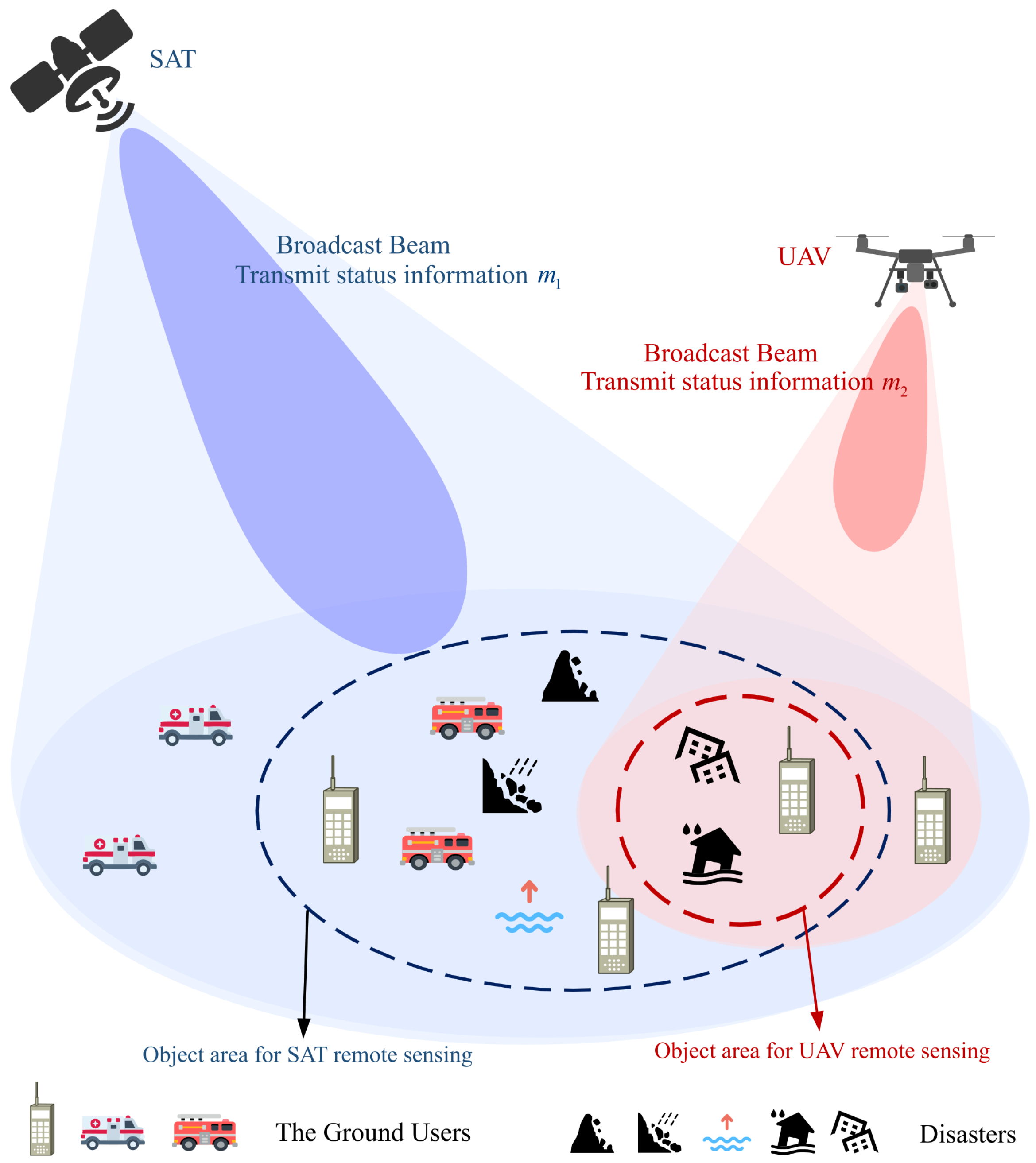
2.1. Scenario

The satellite–UAV “multiscale explanation” synergy real-time sensing scenario is illustrated in Figure 1, which leverages the integrated space–air–ground communication network to provide environmental status information remote sensing and transmission services for military operations, disaster response, relief actions, etc. The satellite, which is recorded as SAT, is dedicated to continuously sensing the status information of a large-scale area, while the UAV focuses on a small-scale area. We assume that there are K GUs in the remote sensing scenario. For brevity, we denote the status information collected by SAT and UAV as $m_1$ and $m_2$, respectively. After each collection, the SAT and UAV immediately transmit the collected information to GUs via broadcast beams. Upon successful transmission of an $m_i$ ($i\in \{1,2\}$) to GU k, the SAT and UAV immediately initiate the next transmission. The GUs, within the beam coverage area, perform fusion processing on the latest received status information to generate the fused status information $m_0$. Considering the spectrum constraints in SAGIN, the FFR strategy is employed by UAV and SAT. The spot beam coverage area of SAT and UAV is, respectively, denoted as $A_{SAT}$ and ${\mathrm{A}}_{UAV}$ that ${\mathrm{A}}_{UAV}\subseteq A_{SAT}$. Additionally, note that in this section, the variables are measured in standard units.

2.2. Communication Model

This subsection presents the communication model under the FFR strategy for the scenario, which mainly includes the channel gain from SAT to GU k in $A_{SAT}$, the channel gain from UAV to GU k in $A_{UAV}$, and the signal to interference plus noise ratio (SINR) at GU k.

2.2.1. The Channel Gain $h_k^s$

The channel gain from SAT to GU k in $A_{SAT}$ is denoted as $h_k^s$. According to [34,35], $h_k^s$ can be expressed as

$$h_k^s=\sqrt{G_s{G}_k{\left({\displaystyle \frac{c}{4\pi f_c{d}_k^s}}\right)}^2},$$

(1)

where $d_k^s$ is the distance between SAT and GU k, $f_c$ is the frequency of operation, c is the speed of light, and $G_s$ and $G_k$, respectively, denote the antenna gain of SAT and GU k. In Equation (1), $G_s$ can be expressed as [36,37,38]

$$G_s\left({\theta }_s\right)=G_{s,max}·{\left({\displaystyle \frac{J_1\left(u_s\right)}{2u_s}}+36{\displaystyle \frac{J_3\left(u_s\right)}{u_s^3}}\right)}^2,$$

(2)

where $u_s=2.07123·sin{\theta }_s/sin{\theta }_{s,3\mathrm{dB}}$, $G_{s,max}$ is the maximum SAT antenna gain, ${\theta }_s$ is the angle between the spot beam center and the location of GU k as seen from the SAT, and $J_1(·)$ and $J_3(·)$, respectively, denote Bessel function of the first kind with order 1 and 3. Without loss of generality, each GU is assumed to equip with an omni-directional antenna.

2.2.2. The Channel Gain $h_k^u$

The channel gain from UAV to GU k in $A_{UAV}$ is denoted as $h_k^u$. It can be expressed as

$$h_k^u=\sqrt{G_u{G}_k{\left({\displaystyle \frac{c}{4\pi f_c{d}_k^u}}\right)}^2},$$

(3)

where $d_k^u$ is the distance between UAV and GU k, and $G_u$ is the UAV antenna gain. According to [39,40], the directional antenna half-power beamwidth of UAV is denoted as $2{\varphi }_u$. Thus, the UAV antenna gain can be approximated by

$$G_u\left({\theta }_u\right)=\left\{\begin{array}{cc}{G}_0/{\varphi }_u^2,\hfill & -{\varphi }_u\le {\theta }_u\le {\varphi }_u,\hfill \\ g_0\approx 0,\hfill & \mathrm{otherwise},\hfill \end{array}\right.$$

(4)

where ${\theta }_u$ is the sector angle, $G_0\approx 29000/2{\varphi }_u$ with ${\varphi }_u$ in degrees [41]. Note that in practice, $g_0$ satisfies $0<g_0\ll G_0/{\varphi }_u^2$, and for simplicity in this paper, $g_0=0$.

2.2.3. SINR

Since the $m_2$ collected by UAV is more correlated to the location of GU k compared to $m_1$ collected by SAT, the reception quality of $m_2$ at GU is prioritized. Therefore, GUs adopt the successive interference cancellation (SIC) to first decode $m_1$ and then decode $m_2$. The SINR of decoding $m_1$ at the GU k in $A_{SAT}$, which is denoted as ${\gamma }_k^s$, can be expressed as

$${\gamma }_k^s={\displaystyle \frac{{\left|\sqrt{p_s}{h}_k^s\right|}^2}{{\left|\sqrt{p_u}{h}_k^u\right|}^2+{\sigma }^2}},k\mathrm{in}{A}_{SAT},$$

(5)

where $p_s$ and $p_u$, respectively, denote the transmit power of SAT and UAV, and ${\sigma }^2$ is the power of additive white Gaussian noise (AWGN). The SINR of decoding $m_2$ at the GU k in $A_{UAV}$, which is denoted as ${\gamma }_k^u$, can be expressed as

$${\gamma }_k^u={\displaystyle \frac{{\left|\sqrt{p_u}{h}_k^u\right|}^2}{{\sigma }^2}},k\mathrm{in}{A}_{UAV},$$

(6)

To ensure that all GUs can correctly decode the packets from the UAV and the SAT, the transmit rate of $m_1$ should be no larger than

$$R_s=B{log}_2\left(1+min\left\{{\gamma }_k^s\mid k\mathrm{in}{A}_{SAT}\right\}\right),$$

(7)

and the transmit rate of $m_2$ should be no larger than

$$R_u=B{log}_2\left(1+min\left\{{\gamma }_k^u\mid k\mathrm{in}{A}_{UAV}\right\}\right),$$

(8)

where B is the FFR bandwidth allocated to SAT and UAV for transmission.

2.3. AoI Analysis Model

This subsection presents the AoI analysis model for fused information corresponding to the scenario described in Section 2.1 and describes the evolution of AoI. As depicted in Figure 2, GU k reserves two queues, queue₁ and queue₂, for storing the received $m_1$ and $m_2$, respectively. GU k generates the fused status information $m_0$ using the $m_1$ and $m_2$ stored at the first position of queue₁ and queue₂ and then discards them immediately. Moreover, define the AoI of the $m_i$ being stored at the jth position of queue_i at time t as ${\Delta }_{m_i}^j\left(t\right)=t-u_{m_i}^j\left(t\right)$, where $u_{m_i}^j\left(t\right)$ is the timestamp. Once GU k generates a new $m_0$, the $m_i$ stored at the head position of queue_i is discarded.

The AoI of the latest fused status information $m_0$, abbreviated as AoI₀, evolves as follows.

$${\mathrm{AoI}}_0\left(t\right)=t-u_{m_0}\left(t\right)+max\left\{{\Delta }_{m_i}^1\left(u_{m_0}\left(t\right)\right)\mid i\in \{1,2\}\right\},$$

(9)

where $u_{m_0}\left(t\right)$ is the timestamp of the latest $m_0$ before time t. Equation (9) indicates that AoI₀$\left(t\right)$ is reset to the larger value between ${\Delta }_{m_1}^1\left(u_{m_0}\left(t\right)\right)$ and ${\Delta }_{m_2}^1\left(u_{m_0}\left(t\right)\right)$ at the completion instant of an $m_0$ generation. Define $M_i$ as the number of transmitted bits for each $m_i$. Typically, $M_i\sim \mathrm{Exp}(1/\overline{M_i})$ with mean $\overline{M_i}$ [42], leading to the transmission time $\Delta t_i$ for each $m_i$, where $\Delta t_i\sim \mathrm{Exp}(1/\overline{\Delta t_i})$ with mean $\overline{\Delta t_i}=\overline{M_i}/R_i$. Therefore, the updating of $m_1$ and $m_2$ can be modeled as two different Poisson processes with rate ${\lambda }_1=R_1/\overline{M_1}$ and ${\lambda }_2=R_2/\overline{M_2}$. Additionally, $m_0$ is generated by GU k as the Poisson process with rate $\mu$.

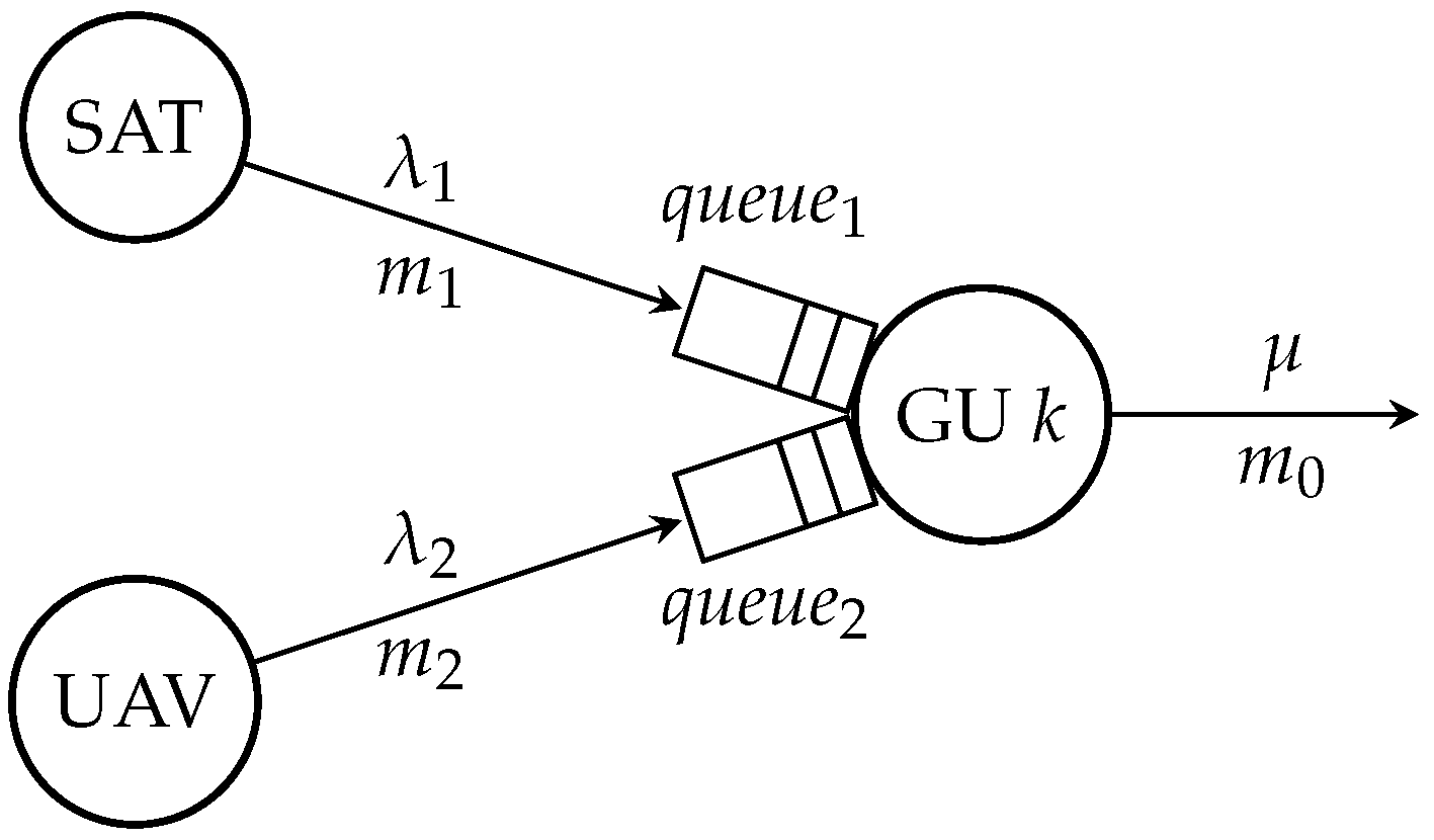
2.4. Queuing Disciplines

To facilitate the study of AoI, the status information update systems are typically modeled as queuing systems, where arriving status information is served following queuing disciplines [43]. In this paper, the AoI₀ performance is analyzed under three queuing disciplines that are commonly considered in research.

Define tuple $\mathbf{a}=(a_1,a_2)$, where $a_1$ denotes the number of $m_1$ currently being stored in queue₁, and $a_2$ denotes the number of $m_2$ stored in queue₂. In the following, the three adopted queuing disciplines are described:

LCFS with no preemption (LCFS-NP): Under the LCFS-NP queuing discipline, queue_i has only one storage position and is non-preemptive. In this paper, for a new arriving $m_1$, if $\mathbf{a}=(0,0)$, the new $m_1$ enters queue₁ and GU k keeps idle. If $\mathbf{a}=(0,1)$, the new $m_1$ enters queue₁ and GU k starts to generate $q_0$ immediately. If $\mathbf{a}=(1,0)$ or $\mathbf{a}=(1,1)$, the new $m_1$ is discarded. For a new arriving $m_2$, it is similar to the above.

LCFS with preemption in service (LCFS-PS): Under the LCFS-PS queuing discipline, queue_i has only one storage position and is preemptive. The new arriving packets are allowed to preempt packets in service and packets in waiting. In this paper, for a new arriving $m_1$, if $\mathbf{a}=(0,0)$, or $\mathbf{a}=(0,1)$, the management of the packet under LCFS-PS is same as the LCFS-NP one. If $\mathbf{a}=(1,0)$, the new $m_1$ preempts the old one stored in queue₁, and the old one is discarded, GU k keeps idle. If $\mathbf{a}=(1,1)$ (i.e., GU k is generating $m_0$), the new $m_1$ preempts the old one stored in queue₁, and the old one is discarded. GU k restarts to generate $m_0$ based on the new $m_1$ and the $m_2$ stored in queue₂. For a new arriving $m_2$, it is similar to the above.

LCFS with preemption in waiting (LCFS-PW): Under the LCFS-PW queuing discipline, queue_i has two storage positions and is preemptive. The new arriving packets are only allowed to preempt packets in waiting. In this paper, for a new arriving $m_1$, if $\mathbf{a}=(0,0)$, or $\mathbf{a}=(0,1)$, or $\mathbf{a}=(1,0)$, the management of the packet under LCFS-PW is the same as the LCFS-PS one. If $\mathbf{a}=(1,1)$ or $\mathbf{a}=(1,2)$, the new $m_1$ enters queue₁. If $\mathbf{a}=(2,1)$ or $\mathbf{a}=(2,2)$, the new $m_1$ preempts the old one stored in the second position of queue₁ and the old one is discarded. For a new arriving $m_2$, it is similar to the above.

In this section, the physical layer communication of the system is built up in the communication model. The information fusion process and the information transmission process are considered in the AoI analysis model. This establishes the relationship between the AoI of fused information and the communication resources of SAGIN. The management for arriving status information is governed by the queuing disciplines. The closed-form expressions of MGF can be derived based on this model, which provide the theoretical basis for AoI analysis in SAGIN in Section 4.

3. Derivation for MGF of AoI₀

3.1. Preliminaries on SHS

Under the three queuing disciplines described in Section 2.4, the queues depicted in Figure 2 are lossy where packets might be preempted or discarded. It is challenging to derive the moments and MGF of AoI₀$\left(t\right)$ in a lossy system by using the graphical approach [8]. Therefore, we solve this problem by utilizing the SHS framework for AoI, which was initially customized by [26,44] for researching AoI.

For the sake of completeness, the main idea of the SHS framework for AoI is briefly presented. In the SHS framework for AoI, the state of a system is partitioned into a discrete component $q\left(t\right)\in \mathcal{Q}=\{0,1,\dots ,w\}$ that evolves as a continuous-time Markov chain and a continuous component $\mathbf{x}$$\left(t\right)=\left[x_0\left(t\right),\cdots ,x_n\left(t\right)\right]$ that describes the evolution processes related to AoI. In the state transition diagram $(\mathcal{Q},\mathcal{L})$ of Markov chain $q\left(t\right)$, each $q\in \mathcal{Q}$ and each transition $l\in \mathcal{L}$ are, respectively, represented as a vertex and a directed edge $\left(q_l,q_l^{\prime }\right)$. Furthermore, the transition rate is ${\lambda }^{\left(l\right)}{\delta }_{q_l,q\left(t\right)}$. It is ensured by the Kronecker delta function ${\delta }_{q_l,q\left(t\right)}$ that the transition l may only occur when $q\left(t\right)=q_l$. For the state $q\in \mathcal{Q}$, the sets ${\mathcal{L}}_q=\left\{l\in \mathcal{L}:q_l=q\right\}$ and ${\mathcal{L}}_q^{\prime }=\left\{l\in \mathcal{L}:q_l^{\prime }=q\right\}$, respectively, denote the collections of outgoing and incoming transitions. As a result of the occurrence of transition l, the system jumps from state $q_l$ to state $q_l^{\prime }$ and resets the continuous component from $\mathbf{x}$ to ${\mathbf{x}}^{\prime }=\mathbf{x}{\mathbf{A}}_l$. ${\mathbf{A}}_l$ is a $(n+1)$-order binary reset map matrix that depends on the characteristics of the specific system. The evolution of continuous component $\mathbf{x}\left(t\right)$ is based on the differential equation $\dot{\mathbf{x}}\left(t\right)=\mathbf{1}$ when $q\left(t\right)=q$. Unlike ordinarily, the SHS may contain self-transitions and multiple transitions. Specifically, self-transitions represent the cases where a reset occurs in the $\mathbf{x}\left(t\right)$ but the $q\left(t\right)$ is unchanged. For the state pair $i,j\in \mathcal{Q}$, multiple transitions represent that the discrete state $q\left(t\right)$ may jump from i to j through transitions with different reset map matrices.

Then, some aspects for deriving MGF using the SHS approach are introduced. ${\pi }_q\left(t\right)$ denotes the probability of being in state $q\in \mathcal{Q}$ at time t. Furthermore, ${\mathbf{v}}_q\left(t\right)$ denotes the correlation vector of $q\left(t\right)$ and $\mathbf{x}\left(t\right)$, and ${\mathbf{v}}_q^{\overline{s}}\left(t\right)$ denotes the correlation vector of $q\left(t\right)$ and $e^{\overline{s}\mathbf{x}\left(t\right)}$, where $\overline{s}\in \mathcal{R}$. ${\widehat{\mathbf{A}}}_l$ is defined as a diagonal companion matrix where if $i=j$ and $[{\mathbf{A}}_l{]}_j={\mathbf{0}}^{\mathsf{T}}$, then $[{\widehat{\mathbf{A}}}_l{]}_{i,j}=1$; otherwise, $[{\widehat{\mathbf{A}}}_l{]}_{i,j}=0$.

$$\begin{array}{c}\hfill {\pi }_q\left(t\right)=\mathbf{E}\left[{\delta }_{q,q\left(t\right)}\right]=Pr[q\left(t\right)=q],\forall q\in \mathcal{Q}\end{array}$$

(10)

$$\begin{array}{c}\hfill {\mathbf{v}}_q\left(t\right)=v_{q0}\left(t\right),\cdots ,v_{qn}\left(t\right)=\mathbf{E}\left[\mathbf{x}\left(t\right){\delta }_{q,q\left(t\right)}\right],\forall q\in \mathcal{Q}\end{array}$$

(11)

$$\begin{array}{c}\hfill {\mathbf{v}}_q^{\overline{s}}\left(t\right)=v_{q0}^{\overline{s}}\left(t\right),\cdots ,v_{qn}^{\overline{s}}\left(t\right)=\mathbf{E}\left[e^{\overline{s}\mathbf{x}\left(t\right)}{\delta }_{q,q\left(t\right)}\right],\forall q\in \mathcal{Q}\end{array}$$

(12)

Based on the ergodicity assumption of Markov chain in [26,44], the probability of state $q\in \mathcal{Q}$ is denoted as $\mathit{\pi }\left(t\right)=\left[\begin{array}{ccc}{\pi }_0\left(t\right),& \cdots ,& {\pi }_w\left(t\right)\end{array}\right]$, which always converges to unique stationary distribution $\overline{\pi }=\left[\begin{array}{ccc}{\overline{\pi }}_0,& \cdots ,& {\overline{\pi }}_w\end{array}\right]$, complying with

$$\begin{array}{c}\hfill {\overline{\pi }}_q\sum _{l\in {\mathcal{L}}_q}{\lambda }^{\left(l\right)}=\sum _{l\in {\mathcal{L}}_q^{\prime }}{\lambda }^{\left(l\right)}{\overline{\pi }}_{q_l},\forall q\in \mathcal{Q},\sum _{q\in \mathcal{Q}}{\overline{\pi }}_q=1.\end{array}$$

(13)

According to ([44], Theorem 1), the MGF $\mathbf{E}\left[e^{\overline{s}\mathbf{x}\left(t\right)}\right]$ converges to $\mathbf{E}\left[e^{\overline{s}\mathbf{x}}\right]$, which can be found by using (14).

$$\begin{array}{cc}\hfill {\overline{\mathbf{v}}}_q^{\overline{s}}\sum _{l\in {\mathcal{L}}_q}{\lambda }^{\left(l\right)}& =s{\overline{\mathbf{v}}}_q^{\overline{s}}+\sum _{l\in {\mathcal{L}}_q^{\prime }}{\lambda }^{\left(l\right)}\left[{\overline{\mathbf{v}}}_{q_l}^{\overline{s}}{\mathbf{A}}_l+{\overline{\pi }}_{q_l}\mathbf{1}{\widehat{\mathbf{A}}}_l\right],\forall q\in \mathcal{Q}\hfill \end{array}$$

(14a)

$$\begin{array}{cc}\hfill \mathbf{E}\left[e^{\overline{s}\mathbf{x}}\right]& =\sum _{q\in \mathcal{Q}}{\overline{v}}_q^{\overline{s}},\mathbf{E}[e^{\overline{s}{x}_0}]=\sum _{q\in \mathcal{Q}}{\overline{v}}_{q0}^{\overline{s}}.\hfill \end{array}$$

(14b)

The n-order moments of $x_0$ are

$$\begin{array}{c}\hfill {\nu }^{\left(n\right)}={\left\{\mathbf{E}\right[e^{\overline{s}{x}_0}\left]{|}_{\overline{s}=0}\right\}}^{\left(n\right)}.\end{array}$$

(15)

3.2. Calculate the MGF of AoI₀ under LCFS-NP

In this subsection, the SHS Markov chain in Figure 3 is built up, which models the discrete state under LCFS-NP. Based on the definitions and notations in Section 3.1, the MGF for the AoI₀ under LCFS-NP is derived by using (13) and (14).

As depicted in Figure 3, when GU k manages the arrived packets under LCFS-NP, the discrete component $q\in \mathcal{Q}=\{0,1,2,3\}$. Each state in $\mathcal{Q}$ represents a potential combination of the numbers of the status information in the queue₁ and queue₂ of GU. For example, a state q = ($a_1$, $a_2$) indicates that the queue₁ at GU has $a_1$ status information $m_1$, and the number of $m_2$ in queue₂ is $a_2$. Note that under the LCFS-NP queuing discipline, if there is already an $m_i$ ($i=1,2$) stored in queue_i, the newly arrived $m_i$ cannot preempt the old one, and the GU discards the newly arrived $m_i$. When q = (1, 1), the GU is busy, which indicates that the GU is performing the fusion of $m_1$ and $m_2$ to generate the fused information $m_0$. When either $a_1$ or $a_2$ is 0, the GU is idle. On the other hand, the continuous component $\mathbf{x}\left(t\right)$ in the system is given by $\mathbf{x}\left(t\right)=\left[x_0\left(t\right),x_1\left(t\right),x_2\left(t\right)\right]$. $x_0\left(t\right)$ captures the continuous-time evolution of AoI₀$\left(t\right)$ in (9); $x_i\left(t\right)$ (i = 1,2) captures the continuous-time AoI evolution of $m_i$ stored in the head position of queue_i and corresponds to ${\Delta }_{m_i}^1\left(u_{m_0}\left(t\right)\right)$ in Equation (9). As long as the discrete state q remains unchanged (i.e., no status information arrives and preempts the old one, or the fused information has been generated), we have ${\displaystyle \frac{\partial \mathbf{x}\left(t\right)}{\partial t}}=1$. This means that the elements recording the age in the vector $\mathbf{x}\left(t\right)$ grow linearly with time.

The transitions are the directed edges $l\in \{1,\cdots ,6\}$. For transitions l,

Table 1. Transitions in Figure 3.

l	${\mathit{q}}_{\mathit{l}}\mathbf{\to }{\mathit{q}}_{\mathit{l}}^{\mathbf{\prime }}$	${\mathit{\lambda }}^{\mathbf{\left(}\mathit{l}\mathbf{\right)}}$	$\mathbf{x}{\mathbf{A}}_{\mathit{l}}$	${\mathbf{A}}_{\mathit{l}}$
1	$0\to 1$	${\lambda }_1$	$\left[\begin{array}{ccc}{x}_0& 0& 0\end{array}\right]$	$\left[\begin{array}{ccc}{\mathbf{m}}_1& {\mathbf{m}}_0& {\mathbf{m}}_0\end{array}\right]$
2	$0\to 2$	${\lambda }_2$	$\left[\begin{array}{ccc}{x}_0& 0& 0\end{array}\right]$	$\left[\begin{array}{ccc}{\mathbf{m}}_1& {\mathbf{m}}_0& {\mathbf{m}}_0\end{array}\right]$
3	$1\to 3$	${\lambda }_2$	$\left[\begin{array}{ccc}{x}_0& x_1& 0\end{array}\right]$	$\left[\begin{array}{ccc}{\mathbf{m}}_1& {\mathbf{m}}_2& {\mathbf{m}}_0\end{array}\right]$
4	$2\to 3$	${\lambda }_1$	$\left[\begin{array}{ccc}{x}_0& 0& x_2\end{array}\right]$	$\left[\begin{array}{ccc}{\mathbf{m}}_1& {\mathbf{m}}_0& {\mathbf{m}}_3\end{array}\right]$
5	$3\to 0$	$\mu$	$\left[\begin{array}{ccc}{x}_1& 0& 0\end{array}\right]$	$\left[\begin{array}{ccc}{\mathbf{m}}_2& {\mathbf{m}}_0& {\mathbf{m}}_0\end{array}\right]$
6	$3\to 0$	$\mu$	$\left[\begin{array}{ccc}{x}_2& 0& 0\end{array}\right]$	$\left[\begin{array}{ccc}{\mathbf{m}}_3& {\mathbf{m}}_0& {\mathbf{m}}_0\end{array}\right]$

presents the transition pair $q_l\to q_l^{\prime }$, the transition rate ${\lambda }^{\left(l\right)}$, the reset map matrix ${\mathbf{A}}_l$, and the transition reset mapping ${\mathbf{x}}^{\prime }=\mathbf{x}{\mathbf{A}}_l$. The directed edge l indicates that transitions from state $q_l$ to $q_l^{\prime }$ occur at rate ${\lambda }^{\left(l\right)}$. Additionally, in this paper, ${\mathbf{m}}_0={\left[\begin{array}{ccc}0& 0& 0\end{array}\right]}^{\mathsf{T}}$, ${\mathbf{m}}_1={\left[\begin{array}{ccc}1& 0& 0\end{array}\right]}^{\mathsf{T}}$, ${\mathbf{m}}_2={\left[\begin{array}{ccc}0& 1& 0\end{array}\right]}^{\mathsf{T}}$, ${\mathbf{m}}_3={\left[\begin{array}{ccc}0& 0& 1\end{array}\right]}^{\mathsf{T}}$. The description of l in Table 1 is as follows.

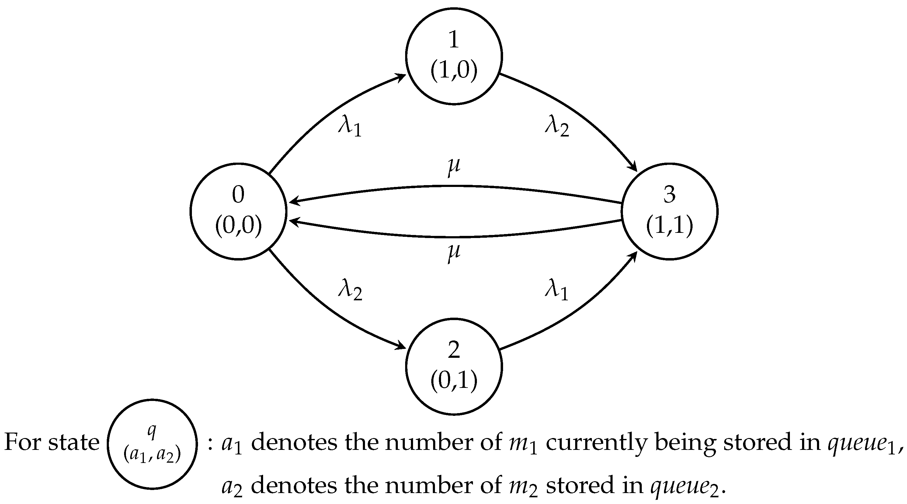
• $l=1$ or 2: In state 0, transition $l=1$ occurs when a new $m_1$ arrives at GU k. ${\mathbf{A}}_l$ governs that $x_0^{\prime }=x_0$ because no new $m_0$ is generated at the end of state 0, $x_1^{\prime }=0$ because the new $m_1$ is fresh, and $x_2^{\prime }=0$ because $x_2$ is irrelevant in state 1. Similarly, the transition $l=2$ occurs when a new $m_2$ arrives. ${\mathbf{A}}_l$ governs that $x_0^{\prime }=x_0$, $x_2^{\prime }=0$, and $x_1^{\prime }=0$;
• $l=3$ or 4: In state 1, the transition $l=3$ occurs when a new $m_2$ arrives at GU k. ${\mathbf{A}}_l$ governs that $x_0^{\prime }=x_0$, $x_1^{\prime }=x_1$ because no new $m_0$ is generated at the end of state 1, and $x_2^{\prime }=0$ because the new $m_2$ is fresh. Similarly, in state 2, the transition $l=4$ occurs when a new $m_1$ arrives. ${\mathbf{A}}_l$ governs that $x_0^{\prime }=x_0$, $x_2^{\prime }=x_2$, and $x_1^{\prime }=0$;
• $l=5$ or 6: In state 3, the transition $l=5$ occurs when a new $m_0$ is generated by GU k and $x_1\left(t\right)>x_2\left(t\right)$ at the same instant. ${\mathbf{A}}_l$ governs that $x_0^{\prime }=x_1$ and governs that {$x_1^{\prime }=0$, $x_2^{\prime }=0$} because the $m_1$ and $m_2$ stored in GU k are discarded when the new $m_0$ is generated. Similarly, the transition $l=6$ occurs when a new $m_0$ is generated and $x_1\left(t\right)$ < $x_2\left(t\right)$ at the same instant. ${\mathbf{A}}_l$ governs that $x_0^{\prime }=x_2$, $x_1^{\prime }=x_0$, and $x_2^{\prime }=0$.

To calculate MGF, the stationary distribution $\overline{\mathit{\pi }}$ is first solved according to (13) and Table 1.

$$\begin{array}{c}\hfill \overline{\mathit{\pi }}=\left[\begin{array}{cccc}{\overline{\pi }}_0& {\overline{\pi }}_1& {\overline{\pi }}_2& {\overline{\pi }}_3\end{array}\right]=\left[\begin{array}{cccc}{\displaystyle \frac{2\mu {\lambda }_1{\lambda }_2}{\alpha }}& {\displaystyle \frac{2\mu {{\lambda }_1}^2}{\alpha }}& {\displaystyle \frac{2\mu {{\lambda }_2}^2}{\alpha }}& {\displaystyle \frac{{\lambda }_1{\lambda }_2({\lambda }_1+{\lambda }_2)}{\alpha }}\end{array}\right],\end{array}$$

(16)

where $\alpha =2\mu ({{\lambda }_1}^2+{{\lambda }_2}^2)+{\lambda }_1{\lambda }_2({\lambda }_1+{\lambda }_2+2\mu )$. Second, equation set (17) is built up according to (14a) and Table 1 to find the matrix $\left[\begin{array}{cccc}{\overline{\mathbf{v}}}_1^{\overline{s}}& {\overline{\mathbf{v}}}_2^{\overline{s}}& \cdots & {\overline{\mathbf{v}}}_m^{\overline{s}}\end{array}\right]$.

$$\begin{array}{cc}\hfill {\overline{\mathbf{v}}}_0^{\overline{s}}({\lambda }_1+{\lambda }_2)& =s{\overline{\mathbf{v}}}_0^{\overline{s}}+\mu \left[\begin{array}{ccc}{\overline{v}}_{31}^{\overline{s}}+{\overline{v}}_{32}^{\overline{s}}& 2{\overline{\pi }}_3& 2{\overline{\pi }}_3\end{array}\right]\hfill \\ \hfill {\overline{\mathbf{v}}}_1^{\overline{s}}{\lambda }_2& =s{\overline{\mathbf{v}}}_0^{\overline{s}}+{\lambda }_1\left[\begin{array}{ccc}{\overline{v}}_{00}^{\overline{s}}+{\overline{v}}_{10}^{\overline{s}}& {\overline{\pi }}_0+{\overline{\pi }}_1& {\overline{\pi }}_0+{\overline{\pi }}_1\end{array}\right]\hfill \\ \hfill {\overline{\mathbf{v}}}_2^{\overline{s}}{\lambda }_1& =s{\overline{\mathbf{v}}}_0^{\overline{s}}+{\lambda }_2\left[\begin{array}{ccc}{\overline{v}}_{00}^{\overline{s}}+{\overline{v}}_{20}^{\overline{s}}& {\overline{\pi }}_0+{\overline{\pi }}_2& {\overline{\pi }}_0+{\overline{\pi }}_2\end{array}\right]\hfill \\ \hfill {\overline{\mathbf{v}}}_3^{\overline{s}}2\mu & =s{\overline{\mathbf{v}}}_0^{\overline{s}}+{\lambda }_2\left[\begin{array}{ccc}{\overline{v}}_{10}^{\overline{s}}+{\overline{v}}_{30}^{\overline{s}}& {\overline{v}}_{11}^{\overline{s}}+{\overline{v}}_{31}^{\overline{s}}& {\overline{\pi }}_1+{\overline{\pi }}_3\end{array}\right]\hfill \\ \hfill & +{\lambda }_1\left[\begin{array}{ccc}{\overline{v}}_{20}^{\overline{s}}+{\overline{v}}_{30}^{\overline{s}}& {\overline{\pi }}_2+{\overline{\pi }}_3& {\overline{v}}_{22}^{\overline{s}}+{\overline{v}}_{32}^{\overline{s}}\end{array}\right].\hfill \end{array}$$

(17)

With some algebraic operations and applying (14b) and (12), the MGF of AoI₀ under LCFS-NP is given by

$$\begin{array}{c}\hfill MG{F}_{NP}\left(\overline{s}\right)={\displaystyle \frac{2{\lambda }_1{\lambda }_2{\mu }^2{\beta }_4{\beta }_5}{{{\beta }_1}^2{{\beta }_2}^2{{\beta }_3}^2\alpha }},\end{array}$$

(18)

where ${\beta }_1=\overline{s}-{\lambda }_1$, ${\beta }_2=\overline{s}-{\lambda }_2$, ${\beta }_3=\overline{s}-2\mu$, ${\beta }_4={\lambda }_2{\beta }_1+{\lambda }_1{\beta }_2$, ${\beta }_5={{\beta }_2}^2{\beta }_3-{\lambda }_1({\beta }_1+{\beta }_2)({\beta }_2-2\mu )$.

According to (15), the mean of AoI₀ under LCFS-NP can be derived as

$$\begin{array}{c}\hfill {\mathrm{AAoI}}_{NP}={\left\{\mathbf{E}\right[MG{F}_{NP}\left(\overline{s}\right)\left]{|}_{\overline{s}=0}\right\}}^{\left(1\right)}.\end{array}$$

(19)

3.3. Calculate the MGF of AoI₀ under LCFS-PS

In this subsection, the SHS Markov chain in Figure 4 is built up, which models the discrete state under LCFS-PS. Then, the MGF for AoI₀ under LCFS-PS is derived.

As depicted in Figure 4, when GU k manages the arrived packets under LCFS-PS, the state $q\in \mathcal{Q}=\{0,1,2,3\}$. The meaning of the discrete component q and the continuous component $\mathbf{x}\left(t\right)$ under LCFS-PS is similar to that under LCFS-NP, as described in Section 3.2. Note that unlike Section 3.2, under the LCFS-PS, newly arrived $m_i$ can preempt the old one already stored in the queue_i at GU, and GU discards the old one. The transitions are labeled $l\in \{1,\dots ,10\}$. The detailed description of the transitions l in

Table 2. Transitions in Figure 4.

l	${\mathit{q}}_{\mathit{l}}\mathbf{\to }{\mathit{q}}_{\mathit{l}}^{\mathbf{\prime }}$	${\mathit{\lambda }}^{\mathbf{\left(}\mathit{l}\mathbf{\right)}}$	$\mathbf{x}{\mathbf{A}}_{\mathit{l}}$	${\mathbf{A}}_{\mathit{l}}$
1	$0\to 1$	${\lambda }_1$	$\left[\begin{array}{ccc}{x}_0& 0& 0\end{array}\right]$	$\left[\begin{array}{ccc}{\mathbf{m}}_1& {\mathbf{m}}_0& {\mathbf{m}}_0\end{array}\right]$
2	$0\to 2$	${\lambda }_2$	$\left[\begin{array}{ccc}{x}_0& 0& 0\end{array}\right]$	$\left[\begin{array}{ccc}{\mathbf{m}}_1& {\mathbf{m}}_0& {\mathbf{m}}_0\end{array}\right]$
3	$1\to 3$	${\lambda }_2$	$\left[\begin{array}{ccc}{x}_0& x_1& 0\end{array}\right]$	$\left[\begin{array}{ccc}{\mathbf{m}}_1& {\mathbf{m}}_2& {\mathbf{m}}_0\end{array}\right]$
4	$2\to 3$	${\lambda }_1$	$\left[\begin{array}{ccc}{x}_0& 0& x_2\end{array}\right]$	$\left[\begin{array}{ccc}{\mathbf{m}}_1& {\mathbf{m}}_0& {\mathbf{m}}_3\end{array}\right]$
5	$3\to 0$	$\mu$	$\left[\begin{array}{ccc}{x}_1& 0& 0\end{array}\right]$	$\left[\begin{array}{ccc}{\mathbf{m}}_2& {\mathbf{m}}_0& {\mathbf{m}}_0\end{array}\right]$
6	$3\to 0$	$\mu$	$\left[\begin{array}{ccc}{x}_2& 0& 0\end{array}\right]$	$\left[\begin{array}{ccc}{\mathbf{m}}_3& {\mathbf{m}}_0& {\mathbf{m}}_0\end{array}\right]$
7	$1\to 1$	${\lambda }_1$	$\left[\begin{array}{ccc}{x}_0& 0& 0\end{array}\right]$	$\left[\begin{array}{ccc}{\mathbf{m}}_1& {\mathbf{m}}_0& {\mathbf{m}}_0\end{array}\right]$
8	$2\to 2$	${\lambda }_2$	$\left[\begin{array}{ccc}{x}_0& 0& 0\end{array}\right]$	$\left[\begin{array}{ccc}{\mathbf{m}}_1& {\mathbf{m}}_0& {\mathbf{m}}_0\end{array}\right]$
9	$3\to 3$	${\lambda }_2$	$\left[\begin{array}{ccc}{x}_0& x_1& 0\end{array}\right]$	$\left[\begin{array}{ccc}{\mathbf{m}}_1& {\mathbf{m}}_2& {\mathbf{m}}_0\end{array}\right]$
10	$3\to 3$	${\lambda }_1$	$\left[\begin{array}{ccc}{x}_0& 0& x_2\end{array}\right]$	$\left[\begin{array}{ccc}{\mathbf{m}}_1& {\mathbf{m}}_0& {\mathbf{m}}_3\end{array}\right]$

is as follows.

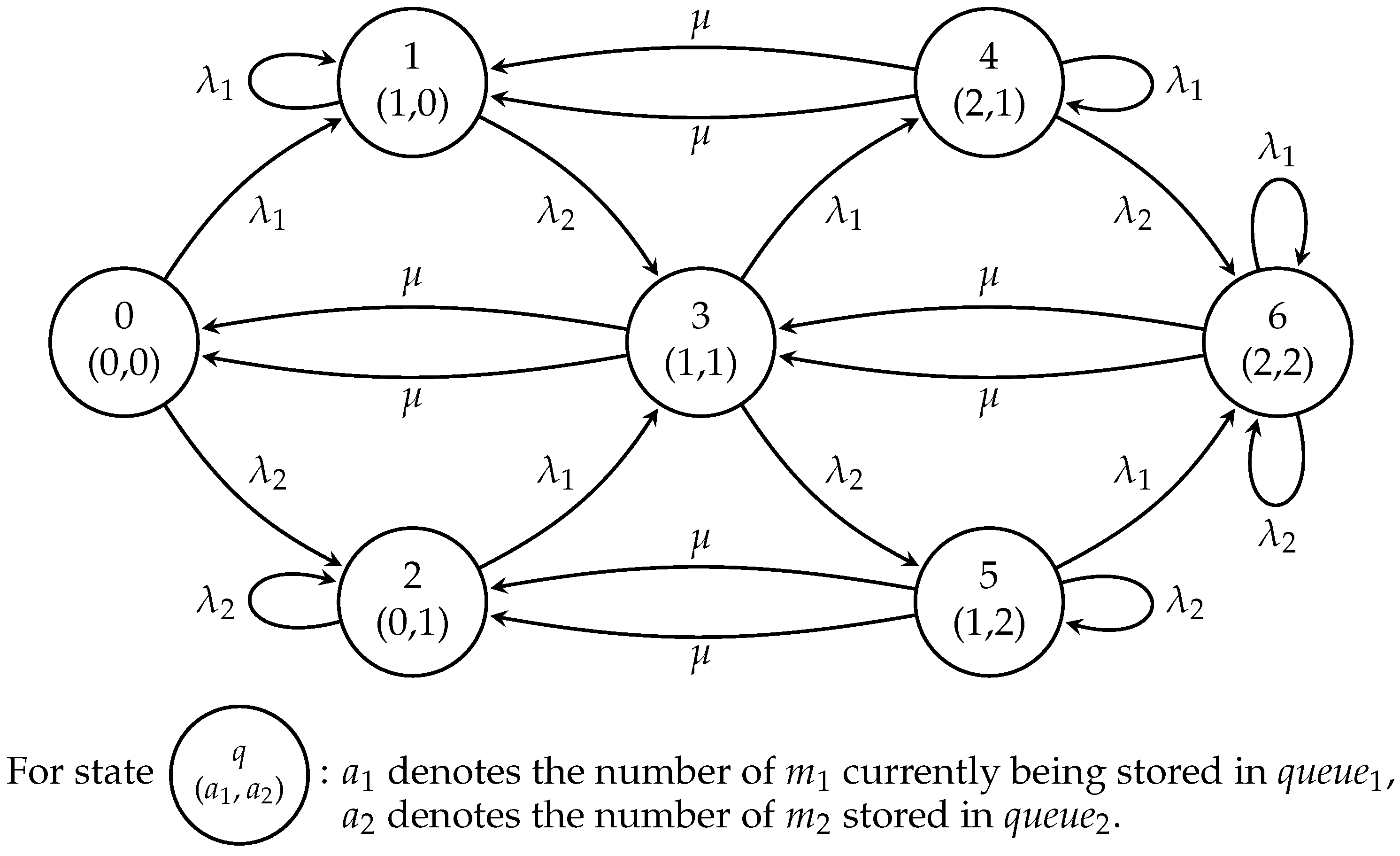
• $l\in \{1,2,3,4,5,6\}$: The descriptions are same as the ones of the transitions $l\in \{1,2,3,4,5,6\}$ in Table 1;
• $l=7$ or 8: In state 1, transition $l=7$ occurs when a new $m_1$ arrives at GU k. The new $m_1$ preempts the old one stored in queue₁. ${\mathbf{A}}_l$ governs that $x_0^{\prime }=x_0$, because no new $m_0$ is generated when the transition occurs, $x_1^{\prime }=0$ because the new $m_1$ is fresh, and $x_2^{\prime }=0$ is due to the irrelevance of $x_2$ to state 1. Similarly, In state 2, the transition occurs when a new $m_2$ arrives, and the new $m_2$ preempts the old one stored in queue₂. ${\mathbf{A}}_l$ governs that $x_0^{\prime }=x_0$, $x_2^{\prime }=0$, and $x_1^{\prime }=0$;
• $l=9$ or 10: In state 3, transition $l=9$ occurs when a new $m_2$ arrives at GU k. The new $m_2$ preempts the old one stored in queue₂. ${\mathbf{A}}_l$ governs that $x_0^{\prime }=x_0$, because no new $m_0$ is generated when the transition occurs, $x_2^{\prime }=0$ because the new $m_2$ is fresh, $x_1^{\prime }=x_1$ because $x_1$ is irrelevant to $m_2$. Similarly, transition $l=10$ occurs when a new $m_1$ arrives. ${\mathbf{A}}_l$ governs that $x_0^{\prime }=x_0$, $x_1^{\prime }=0$, and $x_2^{\prime }=x_2$.

Similar to Section 3.2, with some algebraic operations by using Equations (12)–(14), the MGF of AoI₀ under LCFS-PS is given by

$$\begin{array}{c}\hfill MG{F}_{PS}\left(\overline{s}\right)={\displaystyle \frac{{\lambda }_1{\lambda }_2\mu {\beta }_5({\lambda }_2{\gamma }_2{\gamma }_4+{{\lambda }_1}^3{\gamma }_5+{{\lambda }_1}^2{\gamma }_6+{\lambda }_1{\gamma }_7)}{{\beta }_1{\beta }_2{\beta }_3{{\gamma }_3}^2{\gamma }_1{\gamma }_2\alpha }},\end{array}$$

(20)

where ${\gamma }_1=\overline{s}-{\lambda }_1-2\mu$, ${\gamma }_2=\overline{s}-{\lambda }_2-2\mu$, ${\gamma }_3=-\overline{s}+{\lambda }_1+{\lambda }_2$, ${\gamma }_4=\overline{s}{\lambda }_2+2\overline{s}\mu -4{\lambda }_2\mu$, ${\gamma }_5=-\overline{s}+2{\lambda }_2+4\mu$, ${\gamma }_6={\overline{s}}^2-5\overline{s}{\lambda }_2+4{{\lambda }_2}^2-8\overline{s}\mu +12{\lambda }_2\mu +8{\mu }^2$, ${\gamma }_7=2{\overline{s}}^2{\lambda }_2-5\overline{s}{{\lambda }_2}^2+2{{\lambda }_2}^3+2{\overline{s}}^2\mu -12\overline{s}{\lambda }_2\mu +12{{\lambda }_2}^2\mu -4\overline{s}{\mu }^2+16{\lambda }_2{\mu }^2$.

According to Equation (15), the mean of AoI₀ under the LCFS-PS queuing discipline is derived as ${\mathrm{AAoI}}_{PS}={\left\{\mathbf{E}\right[MG{F}_{PS}\left(\overline{s}\right)\left]{|}_{\overline{s}=0}\right\}}^{\left(1\right)}$.

3.4. Calculate the MGF of AoI₀ under LCFS-PW

In this subsection, the SHS Markov chain in Figure 5 is built up, which models the discrete state under LCFS-PW. Then, the MGF for AoI₀ is derived.

As depicted in Figure 5, when GU k manages the arrived packets under LCFS-PW, the state $q\in \mathcal{Q}=\{0,1,\cdots ,6\}$. The $a_1$ and $a_2$ in the state q = ($a_1$, $a_2$) denote the number of status information stored in queue₁ and queue₂ of GU, respectively. When both $a_1\ge 1$ and $a_2\ge 1$ are true, the GU is busy, indicating that the GU is performing the fusion of $m_1$ and $m_2$ to generate $m_0$. Moreover, when GU is busy, the status information arranged and stored in the second position in queue₁ and queue₂ is in waiting. When either $a_1$ or $a_2$ is 0, the GU is idle, and the status information in queue₁ or queue₂ is in waiting. Under the LCFS-PW, the newly arrived $m_i$ is only able to preempt the old ones that have been stored in queue_i and in waiting. Once a $m_i$ has been preempted, it is discarded by the GU. On the other hand, the continuous component $\mathbf{x}\left(t\right)$ in the system captures the continuous time processes, which are represented by the vector $\mathbf{x}\left(t\right)=\left[x_0\left(t\right),x_1\left(t\right),x_2\left(t\right),x_3\left(t\right),x_4\left(t\right)\right]$. Moreover, $x_0\left(t\right)$ captures the evolution of AoI₀$\left(t\right)$ in Equation (9); $x_{\overline{i}}\left(t\right)$ ($\overline{i}$ = 1,2) captures the evolution of AoI of $m_{\overline{i}}$ stored in the head position of ${\mathit{queue}}_{\overline{i}}$; and $x_{\overline{i}+2}\left(t\right)$ captures the evolution of AoI of $m_{\overline{i}}$ stored in the second position of ${\mathit{queue}}_{\overline{i}}$. Similar to the description in Section 3.2, the elements recording the age in $\mathbf{x}\left(t\right)$ grow linearly with time as long as the discrete state remains unchanged. The transitions $l\in \{1,\dots ,22\}$. For transitions,

Table 3. Transitions in Figure 5.

l	${\mathit{q}}_{\mathit{l}}\mathbf{\to }{\mathit{q}}_{\mathit{l}}^{\mathbf{\prime }}$	${\mathit{\lambda }}^{\mathbf{\left(}\mathit{l}\mathbf{\right)}}$	$\mathbf{x}{\mathbf{A}}_{\mathit{l}}$	${\mathbf{A}}_{\mathit{l}}$
1	$0\to 1$	${\lambda }_1$	$\left[\begin{array}{ccccc}{x}_0& 0& 0& 0& 0\end{array}\right]$	$\left[\begin{array}{ccccc}{\overline{\mathbf{m}}}_1& {\overline{\mathbf{m}}}_0& {\overline{\mathbf{m}}}_0& {\overline{\mathbf{m}}}_0& {\overline{\mathbf{m}}}_0\end{array}\right]$
2	$0\to 2$	${\lambda }_2$	$\left[\begin{array}{ccccc}{x}_0& 0& 0& 0& 0\end{array}\right]$	$\left[\begin{array}{ccccc}{\overline{\mathbf{m}}}_1& {\overline{\mathbf{m}}}_0& {\overline{\mathbf{m}}}_0& {\overline{\mathbf{m}}}_0& {\overline{\mathbf{m}}}_0\end{array}\right]$
3	$1\to 3$	${\lambda }_2$	$\left[\begin{array}{ccccc}{x}_0& x_1& 0& 0& 0\end{array}\right]$	$\left[\begin{array}{ccccc}{\overline{\mathbf{m}}}_1& {\overline{\mathbf{m}}}_2& {\overline{\mathbf{m}}}_0& {\overline{\mathbf{m}}}_0& {\overline{\mathbf{m}}}_0\end{array}\right]$
4	$2\to 3$	${\lambda }_1$	$\left[\begin{array}{ccccc}{x}_0& 0& x_2& 0& 0\end{array}\right]$	$\left[\begin{array}{ccccc}{\overline{\mathbf{m}}}_1& {\overline{\mathbf{m}}}_0& {\overline{\mathbf{m}}}_3& {\overline{\mathbf{m}}}_0& {\overline{\mathbf{m}}}_0\end{array}\right]$
5	$3\to 4$	${\lambda }_1$	$\left[\begin{array}{ccccc}{x}_0& x_1& x_2& 0& 0\end{array}\right]$	$\left[\begin{array}{ccccc}{\overline{\mathbf{m}}}_1& {\overline{\mathbf{m}}}_2& {\overline{\mathbf{m}}}_3& {\overline{\mathbf{m}}}_0& {\overline{\mathbf{m}}}_0\end{array}\right]$
6	$3\to 5$	${\lambda }_2$	$\left[\begin{array}{ccccc}{x}_0& x_1& x_2& 0& 0\end{array}\right]$	$\left[\begin{array}{ccccc}{\overline{\mathbf{m}}}_1& {\overline{\mathbf{m}}}_2& {\overline{\mathbf{m}}}_3& {\overline{\mathbf{m}}}_0& {\overline{\mathbf{m}}}_0\end{array}\right]$
7	$4\to 6$	${\lambda }_2$	$\left[\begin{array}{ccccc}{x}_0& x_1& x_2& x_3& 0\end{array}\right]$	$\left[\begin{array}{ccccc}{\overline{\mathbf{m}}}_1& {\overline{\mathbf{m}}}_2& {\overline{\mathbf{m}}}_3& {\overline{\mathbf{m}}}_4& {\overline{\mathbf{m}}}_0\end{array}\right]$
8	$5\to 6$	${\lambda }_1$	$\left[\begin{array}{ccccc}{x}_0& x_1& x_2& 0& x_4\end{array}\right]$	$\left[\begin{array}{ccccc}{\overline{\mathbf{m}}}_1& {\overline{\mathbf{m}}}_2& {\overline{\mathbf{m}}}_3& {\overline{\mathbf{m}}}_0& {\overline{\mathbf{m}}}_5\end{array}\right]$
9	$1\to 1$	${\lambda }_1$	$\left[\begin{array}{ccccc}{x}_0& 0& 0& 0& 0\end{array}\right]$	$\left[\begin{array}{ccccc}{\overline{\mathbf{m}}}_1& {\overline{\mathbf{m}}}_0& {\overline{\mathbf{m}}}_0& {\overline{\mathbf{m}}}_0& {\overline{\mathbf{m}}}_0\end{array}\right]$
10	$2\to 2$	${\lambda }_2$	$\left[\begin{array}{ccccc}{x}_0& 0& 0& 0& 0\end{array}\right]$	$\left[\begin{array}{ccccc}{\overline{\mathbf{m}}}_1& {\overline{\mathbf{m}}}_0& {\overline{\mathbf{m}}}_0& {\overline{\mathbf{m}}}_0& {\overline{\mathbf{m}}}_0\end{array}\right]$
11	$4\to 4$	${\lambda }_1$	$\left[\begin{array}{ccccc}{x}_0& x_1& x_2& 0& 0\end{array}\right]$	$\left[\begin{array}{ccccc}{\overline{\mathbf{m}}}_1& {\overline{\mathbf{m}}}_2& {\overline{\mathbf{m}}}_3& {\overline{\mathbf{m}}}_0& {\overline{\mathbf{m}}}_0\end{array}\right]$
12	$5\to 5$	${\lambda }_2$	$\left[\begin{array}{ccccc}{x}_0& x_1& x_2& 0& 0\end{array}\right]$	$\left[\begin{array}{ccccc}{\overline{\mathbf{m}}}_1& {\overline{\mathbf{m}}}_2& {\overline{\mathbf{m}}}_3& {\overline{\mathbf{m}}}_0& {\overline{\mathbf{m}}}_0\end{array}\right]$
13	$6\to 6$	${\lambda }_1$	$\left[\begin{array}{ccccc}{x}_0& x_1& x_2& 0& x_4\end{array}\right]$	$\left[\begin{array}{ccccc}{\overline{\mathbf{m}}}_1& {\overline{\mathbf{m}}}_2& {\overline{\mathbf{m}}}_3& {\overline{\mathbf{m}}}_4& {\overline{\mathbf{m}}}_0\end{array}\right]$
14	$6\to 6$	${\lambda }_2$	$\left[\begin{array}{ccccc}{x}_0& x_1& x_2& x_3& 0\end{array}\right]$	$\left[\begin{array}{ccccc}{\overline{\mathbf{m}}}_1& {\overline{\mathbf{m}}}_2& {\overline{\mathbf{m}}}_3& {\overline{\mathbf{m}}}_0& {\overline{\mathbf{m}}}_5\end{array}\right]$
15	$3\to 0$	$\mu$	$\left[\begin{array}{ccccc}{x}_1& 0& 0& 0& 0\end{array}\right]$	$\left[\begin{array}{ccccc}{\overline{\mathbf{m}}}_0& {\overline{\mathbf{m}}}_1& {\overline{\mathbf{m}}}_0& {\overline{\mathbf{m}}}_0& {\overline{\mathbf{m}}}_0\end{array}\right]$
16	$3\to 0$	$\mu$	$\left[\begin{array}{ccccc}{x}_2& 0& 0& 0& 0\end{array}\right]$	$\left[\begin{array}{ccccc}{\overline{\mathbf{m}}}_0& {\overline{\mathbf{m}}}_0& {\overline{\mathbf{m}}}_1& {\overline{\mathbf{m}}}_0& {\overline{\mathbf{m}}}_0\end{array}\right]$
17	$4\to 1$	$\mu$	$\left[\begin{array}{ccccc}{x}_1& x_3& 0& 0& 0\end{array}\right]$	$\left[\begin{array}{ccccc}{\overline{\mathbf{m}}}_0& {\overline{\mathbf{m}}}_1& {\overline{\mathbf{m}}}_0& {\overline{\mathbf{m}}}_2& {\overline{\mathbf{m}}}_0\end{array}\right]$
18	$4\to 1$	$\mu$	$\left[\begin{array}{ccccc}{x}_2& x_3& 0& 0& 0\end{array}\right]$	$\left[\begin{array}{ccccc}{\overline{\mathbf{m}}}_0& {\overline{\mathbf{m}}}_0& {\overline{\mathbf{m}}}_1& {\overline{\mathbf{m}}}_2& {\overline{\mathbf{m}}}_0\end{array}\right]$
19	$5\to 2$	$\mu$	$\left[\begin{array}{ccccc}{x}_1& x_4& 0& 0& 0\end{array}\right]$	$\left[\begin{array}{ccccc}{\overline{\mathbf{m}}}_0& {\overline{\mathbf{m}}}_1& {\overline{\mathbf{m}}}_0& {\overline{\mathbf{m}}}_0& {\overline{\mathbf{m}}}_2\end{array}\right]$
20	$5\to 2$	$\mu$	$\left[\begin{array}{ccccc}{x}_2& x_4& 0& 0& 0\end{array}\right]$	$\left[\begin{array}{ccccc}{\overline{\mathbf{m}}}_0& {\overline{\mathbf{m}}}_0& {\overline{\mathbf{m}}}_1& {\overline{\mathbf{m}}}_0& {\overline{\mathbf{m}}}_2\end{array}\right]$
21	$6\to 3$	$\mu$	$\left[\begin{array}{ccccc}{x}_1& x_3& x_4& 0& 0\end{array}\right]$	$\left[\begin{array}{ccccc}{\overline{\mathbf{m}}}_0& {\overline{\mathbf{m}}}_1& {\overline{\mathbf{m}}}_0& {\overline{\mathbf{m}}}_2& {\overline{\mathbf{m}}}_3\end{array}\right]$
22	$6\to 3$	$\mu$	$\left[\begin{array}{ccccc}{x}_2& x_3& x_4& 0& 0\end{array}\right]$	$\left[\begin{array}{ccccc}{\overline{\mathbf{m}}}_0& {\overline{\mathbf{m}}}_0& {\overline{\mathbf{m}}}_1& {\overline{\mathbf{m}}}_2& {\overline{\mathbf{m}}}_3\end{array}\right]$

presents transition pair $q_l\to q_l^{\prime }$, transition rate ${\lambda }^{\left(l\right)}$, reset map matrix ${\mathbf{A}}_l$, and transition reset mapping ${\mathbf{x}}^{\prime }=\mathbf{x}{\mathbf{A}}_l$. Additionally, in this paper, ${\overline{\mathbf{m}}}_0={\left[\begin{array}{ccccc}0& 0& 0& 0& 0\end{array}\right]}^{\mathsf{T}}$, ${\overline{\mathbf{m}}}_1={\left[\begin{array}{ccccc}1& 0& 0& 0& 0\end{array}\right]}^{\mathsf{T}}$, ${\overline{\mathbf{m}}}_2={\left[\begin{array}{ccccc}0& 1& 0& 0& 0\end{array}\right]}^{\mathsf{T}}$, ${\overline{\mathbf{m}}}_3={\left[\begin{array}{ccccc}0& 0& 1& 0& 0\end{array}\right]}^{\mathsf{T}}$, ${\overline{\mathbf{m}}}_4={\left[\begin{array}{ccccc}0& 0& 0& 1& 0\end{array}\right]}^{\mathsf{T}}$. ${\overline{\mathbf{m}}}_5={\left[\begin{array}{ccccc}0& 0& 0& 0& 1\end{array}\right]}^{\mathsf{T}}$. The essential idea of the transitions l in Table 3 is similar to the ones in Table 1 and Table 2. Therefore, the transitions in Table 3 are not described in detail.

Similar to Section 3.2, with some algebraic operations, the MGF of AoI₀ under LCFS-PW is given by Equation (21).

$$\begin{array}{c}\hfill MG{F}_{PW}\left(\overline{s}\right)={\displaystyle \frac{2{\eta }_1\mu \left(\begin{array}{cc}\hfill & 4{\lambda }_2^2{\mu }^2{\eta }_3^2-{\overline{s}}^3{\eta }_2{\eta }_3{\eta }_4+{\lambda }_1^4{\eta }_5+2{\lambda }_1^3{\eta }_6+2{\lambda }_1{\lambda }_2\mu {\eta }_7+{\lambda }_1^2{\eta }_8\hfill \\ \hfill & -\overline{s}{\lambda }_1{\eta }_{13}+2{\overline{s}}^2({\lambda }_1^3{\eta }_3+2\mu {\eta }_{14}{\eta }_3^2+2{\lambda }_1^2{\eta }_9+{\lambda }_1{\eta }_{10})\hfill \\ \hfill & -\overline{s}({\lambda }_1^4{\eta }_3+2{\lambda }_2\mu {\eta }_{15}{\eta }_3^2+4{\lambda }_1^3{\eta }_{11}+{\lambda }_1^2{\eta }_{12})\hfill \end{array}\right)}{-{\beta }_1{\beta }_2{\beta }_3{\gamma }_3\left(\begin{array}{c}4{\lambda }_2^2{\mu }^2{\eta }_3^2+{\lambda }_1^4{\eta }_5+2{\lambda }_1^3{\eta }_6+2{\lambda }_1{\lambda }_2\mu {\eta }_7+{\lambda }_2^2{\eta }_8\hfill \end{array}\right)}},\end{array}$$

(21)

where ${\eta }_1={\lambda }_1{\lambda }_2({\lambda }_1+{\lambda }_2)$, ${\eta }_2={\lambda }_1+2\mu$, ${\eta }_3={\lambda }_2+2\mu$, ${\eta }_4={\lambda }_1+{\lambda }_2+2\mu$,${\eta }_5={{\lambda }_2}^2+2{\lambda }_2\mu +4{\mu }^2$,${\eta }_6={{\lambda }_2}^3+4{{\lambda }_2}^2\mu +8{\lambda }_2{\mu }^2+8{\mu }^3$, ${\eta }_7={{\lambda }_2}^3+8{{\lambda }_2}^2\mu +16{\lambda }_2{\mu }^2+8{\mu }^3$, ${\eta }_8={{\lambda }_2}^4+8{{\lambda }_2}^3\mu +20{{\lambda }_2}^2{\mu }^2+32{\lambda }_2{\mu }^3+16{\mu }^4$, ${\eta }_9={{\lambda }_2}^2+4{\lambda }_2\mu +5{\mu }^2$, ${\eta }_{10}={{\lambda }_2}^3+8{{\lambda }_2}^2\mu +18{\lambda }_2{\mu }^2+16{\mu }^3$, ${\eta }_{11}={{\lambda }_2}^2+3{\lambda }_2\mu +4{\mu }^2$, ${\eta }_{12}=4{{\lambda }_2}^3+22{{\lambda }_2}^2\mu +44{\lambda }_2{\mu }^2+40{\mu }^3$, ${\eta }_{13}={{\lambda }_2}^4+12{{\lambda }_2}^3\mu +44{{\lambda }_2}^2{\mu }^2+72{\lambda }_2{\mu }^3+32{\mu }^4$, ${\eta }_{14}={\lambda }_2+\mu$, ${\eta }_{15}={\lambda }_2+4\mu$.

According to (15), the mean of AoI₀ under the LCFS-PW queuing discipline is derived as ${\mathrm{AAoI}}_{PW}={\left\{\mathbf{E}\right[MG{F}_{PW}\left(\overline{s}\right)\left]{|}_{\overline{s}=0}\right\}}^{\left(1\right)}$.

Based on the above derivation, Figure 6 briefly compares the average AoI performance under the three queuing disciplines, for ${\lambda }_1=10,{\lambda }_2\in \{1,2,\dots ,10\},\mu =10$. From the figure, it is evident that as parameter ${\lambda }_2$ increases towards ${\lambda }_1$, ${\mathrm{AAoI}}_{NP}$, ${\mathrm{AAoI}}_{PS}$, and ${\mathrm{AAoI}}_{PW}$ decrease. The AAoI initially decreases significantly as the update rate ${\lambda }_2$ increases from zero, and the AoI reduction diminishes as the ${\lambda }_2$ continues to increase. Specifically, as ${\lambda }_2$ increases, ${\mathrm{AAoI}}_{PW}$ becomes lower compared to ${\mathrm{AAoI}}_{NP}$ and ${\mathrm{AAoI}}_{PS}$, signifying better AoI performance from the LCFS-PW. In the next section, the ${\mathrm{AAoI}}_{PW}$-related performance is simulated and analyzed in the satellite and UAV synergy remote sensing scenario.

4. Numerical Results

This section analyzes and compares the AAoIPW-related performance in the SAGIN remote sensing system. The system consists of a low earth orbit (LEO) satellite and a UAV as information sources and ground users (GUs) as information receivers. These GUs continuously receive status information from both sources and perform multiscale information fusion. Considering the limited spectrum resources in real SAGIN, the FFR strategy is employed in the system. Under the FFR strategy, GUs adopt successive interference cancellation (SIC) to first decode the information from the UAV and then decode the information from the satellite. Since satellite and UAV nodes are sensitive to the transmission energy consumption and system bandwidth resources in the SAGIN remote sensing system, here, we mainly focus on the impact of transmission power and bandwidth.

The main simulation parameters of SAT are presented in

Table 4. Simulation Parameters.

Parameter of SAT [45]	Value
Orbital height (LEO)	$H_s=600\mathrm{km}\left(\mathrm{LEO}\right)$
3 dB beamwidth	${\theta }_{s,3\mathrm{dB}}=8.8320°$
Beam diameter	$r_s=45\mathrm{km}$
Downlink carrier frequency	$f_c=2\mathrm{GHz}$ (S-band)
Satellite maximum antenna gain	$G_{s,max}=24\mathrm{dBi}$
Parameter of UAV	Value
Altitude of UAV	$H_u=5\mathrm{km}$
Half beamwidth of UAV	${\varphi }_u=80°$ [39]

. According to the technical reports of the 3rd Generation Partnership Project (3GPP) [45], for SAT, set orbital height $H_s=600\mathrm{km}$, 3 dB beamwidth ${\theta }_{s,3\mathrm{dB}}=8.83°$, beam diameter $r_u=45\mathrm{km}$, and maximum gain $G_{s,max}=24$ dBi. For UAV, set altitude $H_u=5\mathrm{km}$, and half beamwidth ${\varphi }_u=80°$. The downlink carrier frequency in system $f_c=2$ GHz. Moreover, the receiver noise temperature for the GUs is set as 24 $\mathrm{dBK}$ [46]. Without loss of generality, the bandwidths allocated to SAT and UAV are equal under FDMA. Additionally, $\overline{M_1}=\overline{M_2}=2\ast {10}^6$. ${\mathrm{AAoI}}_{PW}^{FF}$ and ${\mathrm{AAoI}}_{PW}^{FD}$, respectively, denote the ${\mathrm{AAoI}}_{PW}$ under FFR and FDMA. Unless stated otherwise, in the simulation environment, the magnitudes of the variables are set to standard units.

Figure 7 shows the performance of ${\mathrm{AAoI}}_{PW}^{FD}$ and ${\mathrm{AAoI}}_{PW}^{FF}$ versus $p_u$, for $p_s\in \{40,43,45\}$ dbm, $p_u\in \{0,2,4,\dots ,28,30\}$ dbm, and B = 2 MHz. From the red line in the figure, the ${\mathrm{AAoI}}_{PW}^{FF}$ initially experiences a decline followed by an incline as $p_u$ increases. The inclining trend is due to the augmented interference with the SAT-GU link resulting from the increased $p_u$ of the UAV at a lower altitude. Consequently, the SAT’s status information update rate ${\lambda }_1$ decreases, leading to a deterioration in ${\mathrm{AAoI}}_{PW}^{FF}$. It can be further noted that increasing $p_s$ decreases minimum ${\mathrm{AAoI}}_{PW}^{FF}$ and the $p_u$ value corresponding to minimum ${\mathrm{AAoI}}_{PW}^{FF}$ increases. This is owing to the fact that increasing $p_s$ improves the update rate ${\lambda }_1$ and mitigates interference from UAV. Nevertheless, due to stringent power constraints for individual beams of the satellite, enhancing ${\mathrm{AAoI}}_{PW}^{FF}$ performance through increasing $p_s$ is a cost-ineffective approach. Moreover, under the FDMA strategy, the UAV signals do not interfere with the SAT signals, resulting in a limited impact of $p_u$ on ${\mathrm{AAoI}}_{PW}^{FD}$. Furthermore, as $p_u$ increases, the relative performance advantage of ${\mathrm{AAoI}}_{PW}^{FF}$ over ${\mathrm{AAoI}}_{PW}^{FD}$ diminishes progressively. The above analysis can provide a reference for the design of power control algorithms that dynamically adjust the transmit power of satellites and UAVs in SAGIN based on real-time channel conditions to optimize AoI. Such algorithms are particularly important in dense urban or disaster scenarios where interference is more likely to degrade communication quality.

In the following content, define the relative performance advantage of ${\mathrm{AAoI}}_{PW}^{FF}$ over ${\mathrm{AAoI}}_{PW}^{FD}$ as ${\mathrm{AAoI}}_{advan}$ = $-({\mathrm{AAoI}}_{PW}^{FF}-{\mathrm{AAoI}}_{PW}^{FD})$, which quantifies the advantage of the FFR strategy over the FDMA strategy in terms of ${\mathrm{AAoI}}_{PW}$. Moreover, the metric energy advantage (EA) is defined to evaluate ${\mathrm{AAoI}}_{advan}$ per unit transmit power in this paper. The EA with respect to $p_u$ and $p_s$ is calculated as

$$\begin{array}{c}\hfill \mathrm{EA}(p_u,p_s,B)={\displaystyle \frac{{\mathrm{AAoI}}_{advan}}{{10}^{(p_s-30)/10}+{10}^{(p_u-30)/10}}}.\end{array}$$

(22)

To clearly illustrate the numerical differences in energy advantage under various parameter settings, we converted the units of $p_s$ and $p_u$ from dBm to Watts through ${10}^{(p_s-30)/10}$ and ${10}^{(p_u-30)/10}$.

Similarly, define the metric spectrum advantage (SA) to evaluate ${\mathrm{AAoI}}_{advan}$ per unit spectrum resource in this paper. The SA with respect to B is calculated as

$$\begin{array}{c}\hfill \mathrm{SA}(p_u,p_s,B)={\displaystyle \frac{{\mathrm{AAoI}}_{advan}}{B}}\end{array}$$

(23)

In Figure 8, EA > 0 indicates that under the current settings of $p_u$ and $p_s$, the FFR strategy outperforms FDMA in ${\mathrm{AAoI}}_{advan}$ per unit transmit power. This indicates that under these settings, the FFR strategy exhibits superior energy efficiency compared to FDMA. It verifies that FFR can be a preferable strategy in scenarios where energy resources are constrained, such as in battery-operated UAVs or power-limited satellites. As $p_s$ increases, more energy is consumed, leading to a decrease in EA. This is due to the fact that it is inefficient to reduce the AoI by increasing the rate of only one Poisson process. However, when more $p_s$ is spent, EA is still above 0, especially when $p_u$ < 15 dBm. This is mainly due to two reasons. On the one hand, the FFR strategy can improve the spectrum efficiency and network throughput in SAGIN, which improves the AoI performance. On the other hand, appropriately increasing $p_s$ can improve the SINR of the SAT-GU channel, which mitigates the effects of interference from the UAV-GU channel to the SAT-GU channel and then enhances the resistance of the satellite signal. This improves the communication rate of the SAT-UAV channel and, to some extent, improves the AoI performance of the fused information at GU under the FFR strategy. This insight suggests that power control strategies should be an integral part of network design. In practice, the AoI of fused remote sensing information in the SAGIN network can be improved by deploying the power control mechanism to adjust the satellite power output according to the real-time interference level. Additionally, as $p_u$ increases, the interference from the UAV-GU channel to the SAT-GU channel increases, thereby reducing EA. For example, as shown by the blue line in Figure 8, when $p_s$ = 45 dBm and $p_u$ > 21 dBm, EA becomes less than 0. The reduced EA at high $p_u$ highlights the significance of interference management in SAGIN. Techniques such as interference cancellation, beamforming, and advanced modulation schemes could be employed to reduce the impact interference, thereby further improving the AoI performance of fused information in SAGIN.

Figure 9 studies the impact of bandwidth B on the spectrum advantage SA, for $p_s\in \{43,45\}$ dBm, $p_u\in \{13,18,23\}$ dBm, and $B\in \{2,3,4,5,6\}$ MHz. When both $p_u\le 18$ dBm and $p_s\ge 42$ dBm, SA > 0, which indicates that the FFR strategy outperforms FDMA in ${\mathrm{AAoI}}_{advan}$ per unit spectrum resource. Under the FFR strategy, interference from the UAV-GU channel to the SAT-GU channel can be mitigated by setting $p_u$ and $p_s$ appropriately to fully utilize spectrum resources and improve system throughput. This, in turn, increases the status information update rate and improves the ${\mathrm{AAoI}}_{PW}$ and SA. The above analysis informs that in spectrum-constrained scenarios such as rural areas lacking infrastructure, the FFR strategy allows for better utilization of available spectrum, leading to improved system throughput and AoI performance. Moreover, SA gradually decreases with the increase in B. This trend suggests that the advantage of FFR in terms of spectrum efficiency diminishes when the spectrum resource is sufficient. It further informs that FFR is beneficial in scenarios with constrained spectrum. On the other hand, when $p_u$ > 18 dBm or $p_s$ < 42 dBm, SA < 0. Under the FFR strategy, either small $p_s$ or large $p_u$ leads to significant interference from UAV-GU channel to SAT-GU channel, which deteriorates the system throughput and SA. Although increasing B improves SA, the benefit is not significant. This is obviously because more spectrum resources have to be allocated. The insights observed from above analysis of SA can provide a reference for spectrum management strategies in SAGIN. For example, in SAGIN, dynamic adjustment of spectrum allocation based on the current power settings and interference levels can optimize network performance. In practice, this could mean deploying cognitive radio techniques that allow the network to dynamically sense and adapt to varying interference, thereby optimizing spectrum efficiency and improving network performance such as AoI.

Based on the comprehensive analysis of Figure 7, Figure 8 and Figure 9, it can be concluded that optimizing AAoI-related performance requires the judicious selection of transmit power to effectively utilize constrained power and spectrum resources. Moreover, the analysis shows the advantages of FFR in SAGIN and highlights the requirement for adaptive management strategies in SAGIN. For the satellite–UAV synergy remote sensing application in SAGIN, it is necessary to dynamically adjust the transmit power and spectrum allocation according to the real-time network environment to optimize system energy efficiency, spectrum efficiency, AoI, etc., ensuring that quality of service is satisfied while avoiding the waste of resources. The future research could focus on developing intelligent algorithms that leverage machine learning to predict and respond to the complex and dynamic network environment in SAGIN. This would enable more efficient and effective resource management. Furthermore, the analysis highlights the critical role of interference management in SAGIN. It is essential to explore technologies such as beamforming, interference cancellation, and advanced modulation schemes to mitigate the impact of interference, especially in disaster areas, rural areas, and battlefield electromagnetic environment.

5. Conclusions

In this paper, a comprehensive analysis of AoI is carried out for the real-time “multiscale explanation” information fusion in the satellite–UAV synergy remote sensing system. The closed-form expression of mean AoI for the fused status information in the system is derived. Based on the closed-form expression, AoI performance, energy advantage, and spectrum advantage of FFR strategy over the FDMA strategy are analyzed. The analysis shows that the FFR strategy yields improved AoI-related performance, especially under spectrum-constrained conditions and within some commonly used transmit power ranges. Moreover, the analysis results emphasize the requirement for adaptive power control strategies, spectrum management strategies, and interference management strategies in SAGIN. The proposed analytical methodology holds significant value for the examination and optimization of AoI for the real-time remote sensing system in SAGIN. It provides a robust framework for assessing the impact of various queuing disciplines and communication strategies on the freshness of information, thereby facilitating the development of more efficient and effective remote sensing systems.

Given the promising findings of this study, it is essential to address the practical limitations and challenges that arise in real-world applications. The future work should focus on addressing practical challenges, such as the limitations of UAVs in terms of battery management and susceptibility to weather conditions, as well as the constraints of LEO satellite systems, including limited communication time. To enhance the applicability of the proposed methodology in real-time systems, the future works will explore the development of adaptive energy and spectrum management strategies, robust UAV path planning algorithms that account for environmental variability, and optimized rate transition and sampling time strategies. These efforts will ensure the proposed methods can be effectively applied in dynamic and unpredictable real-world environments.

References

- Lu, H.; Gui, Y.; Jiang, X.; Wu, F.; Chen, C.W. Compressed robust transmission for remote sensing services in space information networks. IEEE Wirel. Commun. 2019, 26, 46–54. [Google Scholar] [CrossRef]
- Zhu, X.; Jiang, C. Integrated satellite-terrestrial networks toward 6G: Architectures, applications, and challenges. IEEE Internet Things J. 2021, 9, 437–461. [Google Scholar] [CrossRef]
- Gui, J.; Cai, F. Coverage probability and throughput optimization in integrated mmWave and Sub-6 GHz multi-UAV-assisted disaster relief networks. IEEE Trans. Mob. Comput. 2024. [Google Scholar] [CrossRef]
- Alvarez-Vanhard, E.; Corpetti, T.; Houet, T. UAV & satellite synergies for optical remote sensing applications: A literature review. Sci. Remote Sens. 2021, 3, 100019. [Google Scholar]
- Lei, T.; Wang, J.; Li, X.; Wang, W.; Shao, C.; Liu, B. Flood disaster monitoring and emergency assessment based on multi-source remote sensing observations. Water 2022, 14, 2207. [Google Scholar] [CrossRef]
- Lei, T.; Cheng, H.; Li, A.; Qu, W.; Pang, Z.; Fu, J.; Li, L.; Li, X.; Lu, J. Cooperative emergency monitoring and assessment of flood disasters based on the integrated ground-air-space remote sensing. In Proceedings of the IGARSS 2019—2019 IEEE International Geoscience and Remote Sensing Symposium, Yokohama, Japan, 28 July–2 August 2019; IEEE: Piscataway, NJ, USA, 2019; pp. 9733–9736. [Google Scholar]
- Zhou, B.; Saad, W. On the age of information in Internet of Things systems with correlated devices. In Proceedings of the GLOBECOM 2020—2020 IEEE Global Communications Conference, Taipei, Taiwan, 7–11 December 2020; IEEE: Piscataway, NJ, USA, 2020; pp. 1–6. [Google Scholar]
- Sun, Y.; Uysal-Biyikoglu, E.; Yates, R.D.; Koksal, C.E.; Shroff, N.B. Update or wait: How to keep your data fresh. IEEE Trans. Inf. Theory 2017, 63, 7492–7508. [Google Scholar] [CrossRef]
- Yates, R.D.; Sun, Y.; Brown, D.R.; Kaul, S.K.; Modiano, E.; Ulukus, S. Age of information: An introduction and survey. IEEE J. Sel. Areas Commun. 2021, 39, 1183–1210. [Google Scholar] [CrossRef]
- Kaul, S.; Yates, R.; Gruteser, M. Real-time status: How often should one update? In Proceedings of the 2012 Proceedings IEEE INFOCOM, Orlando, FL, USA, 25–30 March 2012; IEEE: Piscataway, NJ, USA, 2012; pp. 2731–2735. [Google Scholar]
- Long, Y.; Zhao, S.; Gong, S.; Gu, B.; Niyato, D.; Shen, X. AoI-aware Sensing Scheduling and Trajectory Optimization for Multi-UAV-assisted Wireless Backscatter Networks. IEEE Trans. Veh. Technol. 2024. [Google Scholar] [CrossRef]
- Zhu, B.; Bedeer, E.; Nguyen, H.H.; Barton, R.; Gao, Z. UAV trajectory planning for AoI-minimal data collection in UAV-aided IoT networks by transformer. IEEE Trans. Wirel. Commun. 2022, 22, 1343–1358. [Google Scholar] [CrossRef]
- Li, M.; Jia, G.; Li, X.; Qiu, H. Efficient Trajectory Planning for Optimizing Energy Consumption and Completion Time in UAV-Assisted IoT Networks. Mathematics 2023, 11, 4399. [Google Scholar] [CrossRef]
- Liu, C.; Guo, Y.; Li, N.; Song, X. AoI-minimal task assignment and trajectory optimization in multi-UAV-assisted IoT networks. IEEE Internet Things J. 2022, 9, 21777–21791. [Google Scholar] [CrossRef]
- Samir, M.; Assi, C.; Sharafeddine, S.; Ghrayeb, A. Online altitude control and scheduling policy for minimizing AoI in UAV-assisted IoT wireless networks. IEEE Trans. Mob. Comput. 2020, 21, 2493–2505. [Google Scholar] [CrossRef]
- Ngo, Q.T.; Tang, Z.; Jayawickrama, B.; He, Y.; Dutkiewicz, E.; Senanayake, B. Timeliness of Information in 5G Non-Terrestrial Networks: A Survey. IEEE Internet Things J. 2024. [Google Scholar] [CrossRef]
- Yuan, A.; Hu, Z.; Zhang, Q.; Sun, Z.; Yang, Z. Towards the age in Cislunar Communication: An AoI-Optimal Multi-Relay Constellation with Heterogeneous Orbits. IEEE J. Sel. Areas Commun. 2024, 42, 1420–1435. [Google Scholar] [CrossRef]
- Kaul, S.; Gruteser, M.; Rai, V.; Kenney, J. Minimizing age of information in vehicular networks. In Proceedings of the 2011 8th Annual IEEE Communications Society Conference on Sensor, Mesh and Ad Hoc Communications and Networks, Salt Lake City, UT, USA, 27–30 June 2011; IEEE: Piscataway, NJ, USA, 2011; pp. 350–358. [Google Scholar]
- Popovski, P.; Chiariotti, F.; Huang, K.; Kalør, A.E.; Kountouris, M.; Pappas, N.; Soret, B. A perspective on time toward wireless 6G. Proc. IEEE 2022, 110, 1116–1146. [Google Scholar] [CrossRef]
- Kosta, A.; Pappas, N.; Angelakis, V. Age of information: A new concept, metric, and tool. Found. Trends Netw. 2017, 12, 162–259. [Google Scholar] [CrossRef]
- Costa, M.; Codreanu, M.; Ephremides, A. Age of information with packet management. In Proceedings of the 2014 IEEE International Symposium on Information Theory, Honolulu, HI, USA, 29 June–4 July 2014; IEEE: Piscataway, NJ, USA, 2014; pp. 1583–1587. [Google Scholar]
- Costa, M.; Codreanu, M.; Ephremides, A. On the age of information in status update systems with packet management. IEEE Trans. Inf. Theory 2016, 62, 1897–1910. [Google Scholar] [CrossRef]
- Kam, C.; Kompella, S.; Ephremides, A. Age of information under random updates. In Proceedings of the 2013 IEEE International Symposium on Information Theory, Istanbul, Turkey, 7–12 July 2013; IEEE: Piscataway, NJ, USA, 2013; pp. 66–70. [Google Scholar]
- Kam, C.; Kompella, S.; Nguyen, G.D.; Ephremides, A. Effect of message transmission path diversity on status age. IEEE Trans. Inf. Theory 2015, 62, 1360–1374. [Google Scholar] [CrossRef]
- Yates, R.D. Status updates through networks of parallel servers. In Proceedings of the 2018 IEEE International Symposium on Information Theory (ISIT), Vail, CO, USA, 17–22 June 2018; IEEE: Piscataway, NJ, USA, 2018; pp. 2281–2285. [Google Scholar]
- Yates, R.D.; Kaul, S.K. The age of information: Real-time status updating by multiple sources. IEEE Trans. Inf. Theory 2018, 65, 1807–1827. [Google Scholar] [CrossRef]
- Najm, E.; Telatar, E. Status updates in a multi-stream M/G/1/1 preemptive queue. In Proceedings of the IEEE Infocom 2018-IEEE Conference On Computer Communications Workshops (Infocom Wkshps), Honolulu, HI, USA, 15–19 April 2018; IEEE: Piscataway, NJ, USA, 2018; pp. 124–129. [Google Scholar]
- Moltafet, M.; Leinonen, M.; Codreanu, M. On the age of information in multi-source queueing models. IEEE Trans. Commun. 2020, 68, 5003–5017. [Google Scholar] [CrossRef]
- Kaul, S.K.; Yates, R.D. Timely updates by multiple sources: The M/M/1 queue revisited. In Proceedings of the 2020 54th Annual Conference on Information Sciences and Systems (CISS), Princeton, NJ, USA, 18–20 March 2020; IEEE: Piscataway, NJ, USA, 2020; pp. 1–6. [Google Scholar]
- Maatouk, A.; Assaad, M.; Ephremides, A. Age of information with prioritized streams: When to buffer preempted packets? In Proceedings of the 2019 IEEE International Symposium on Information Theory (ISIT), Paris, France, 7–12 July 2019; IEEE: Piscataway, NJ, USA, 2019; pp. 325–329. [Google Scholar]
- Chiang, Y.H.; Lin, H.; Ji, Y. Information cofreshness-aware grant assignment and transmission scheduling for internet of things. IEEE Internet Things J. 2021, 8, 14435–14446. [Google Scholar] [CrossRef]
- Pan, W.; Deng, Z.; Wang, X.; Zhou, P.; Wu, W. Optimizing the age of information for multi-source information update in Internet of Things. IEEE Trans. Netw. Sci. Eng. 2022, 9, 904–917. [Google Scholar] [CrossRef]
- Yan, Y.; Wang, Y.; Zhao, J.; Ni, W. Request oriented cache update for age of information minimization in industrial control systems. In Proceedings of the ICC 2023-IEEE International Conference on Communications, Rome, Italy, 28 May–1 June 2023; IEEE: Piscataway, NJ, USA, 2023; pp. 1774–1779. [Google Scholar]
- Gao, Z.; Liu, A.; Liang, X. Data transmission time minimization for LEO satellite-terrestrial integrated networks. In Proceedings of the 2020 International Conference on Wireless Communications and Signal Processing (WCSP), Nanjing, China, 21–23 October 2020; IEEE: Piscataway, NJ, USA, 2020; pp. 642–647. [Google Scholar]
- Han, C.; Liu, A.; Wang, H.; Huo, L.; Liang, X. Dynamic anti-jamming coalition for satellite-enabled army IoT: A distributed game approach. IEEE Internet Things J. 2020, 7, 10932–10944. [Google Scholar] [CrossRef]
- Huang, Q.; Lin, M.; Wang, J.B.; Tsiftsis, T.A.; Wang, J. Energy efficient beamforming schemes for satellite-aerial-terrestrial networks. IEEE Trans. Commun. 2020, 68, 3863–3875. [Google Scholar] [CrossRef]
- Zheng, G.; Chatzinotas, S.; Ottersten, B. Generic optimization of linear precoding in multibeam satellite systems. IEEE Trans. Wirel. Commun. 2012, 11, 2308–2320. [Google Scholar] [CrossRef]
- Guo, K.; Lin, M.; Zhang, B.; Zhu, W.P.; Wang, J.B.; Tsiftsis, T.A. On the performance of LMS communication with hardware impairments and interference. IEEE Trans. Commun. 2018, 67, 1490–1505. [Google Scholar] [CrossRef]
- Mozaffari, M.; Saad, W.; Bennis, M.; Debbah, M. Efficient deployment of multiple unmanned aerial vehicles for optimal wireless coverage. IEEE Commun. Lett. 2016, 20, 1647–1650. [Google Scholar] [CrossRef]
- He, H.; Zhang, S.; Zeng, Y.; Zhang, R. Joint altitude and beamwidth optimization for UAV-enabled multiuser communications. IEEE Commun. Lett. 2017, 22, 344–347. [Google Scholar] [CrossRef]
- Balanis, C.A. Antenna Theory: Analysis and Design; John Wiley & Sons: Hoboken, NJ, USA, 2016. [Google Scholar]
- Lei, L.; Xu, H.; Xiong, X.; Zheng, K.; Xiang, W. Joint computation offloading and multiuser scheduling using approximate dynamic programming in NB-IoT edge computing system. IEEE Internet Things J. 2019, 6, 5345–5362. [Google Scholar] [CrossRef]
- Inoue, Y.; Masuyama, H.; Takine, T.; Tanaka, T. A general formula for the stationary distribution of the age of information and its application to single-server queues. IEEE Trans. Inf. Theory 2019, 65, 8305–8324. [Google Scholar] [CrossRef]
- Yates, R.D. The age of information in networks: Moments, distributions, and sampling. IEEE Trans. Inf. Theory 2020, 66, 5712–5728. [Google Scholar] [CrossRef]
- 3GPP, Solutions for NR to Support Non-Terrestrial Networks (NTN). 3rd Generation Partnership Project (3GPP), Technical Report (TR) 38.821, May 2021, Version 16.1.0. Available online: https://portal.3gpp.org/desktopmodules/Specifications/SpecificationDetails.aspx?specificationId=3525 (accessed on 27 July 2024).
- Palacios, J.; González-Prelcic, N.; Mosquera, C.; Shimizu, T.; Wang, C.H. A hybrid beamforming design for massive MIMO LEO satellite communications. Front. Space Technol. 2021, 2, 696464. [Google Scholar] [CrossRef]