Target Motion Parameters Estimation by Full-Plane Hyperbola-Warping Transform with a Single Hydrophone

Abstract

In this paper, to counteract the sensitivity of the traditional Hough transform to noise and the fluctuations in parameter estimation, we propose a hyperbolic warping transform that integrates all interference fringes in the time–frequency domain to accurately estimate the motion parameters of a single hydrophone. This method can accurately estimate the target motion parameters, including the time of closest point of approach ($t_{CPA}$), the ratio of the nearest distance to the speed ($b=r_{CPA}/v$), and the waveguide invariant ($\beta$). The two algorithms are compared by simulation and sea trial experiments. Hyperbola-warping improves the noise immunity performance by 10 dB in simulation experiments, increases the detection range by 20% in sea trial experiments, and demonstrates that the method proposed in this paper has better noise resistance and practicality.

1. Introduction

When an acoustic signal propagates in the shallow-water waveguide, each normal mode interferes with the other to form a stable interference structure. The interference structure contains a large amount of target information and marine environment information. Therefore, how to use the interference structure to obtain target parameters [1,2] and marine environment inversion [3,4] has become an important research content in the field of underwater acoustics in recent years. Li et al. [5] proposed an extraction and phase compensation method based on the time–frequency spectrogram, and the acoustic data obtained can be used for source ranging. Song et al. [6], observing a sudden change in the waveguide invariant from the time–frequency spectrum data in sea trial experiments, proposes a new model that accounts for the source’s movement in a gradually varying range and azimuth within a non-radial waveguide. Song et al. [7] presented a method for estimating the range of a distant ship in shallow water, utilizing a vertical array and a guide ship at a known range near the array, by integrating four distinct approaches: blind deconvolution, waveguide invariant, virtual receiver (VR), and array invariant.

Compared with the three sub-array method [8,9,10], target motion analysis (TMA) [11,12], matching field [13] and other methods [14,15], single hydrophone target parameter estimation does not require a large hydrophone array and a large number of sound field calculations, so it has become a research hotspot for scholars at home and abroad.

Current common methods for underwater target parameter estimation using a single hydrophone primarily rely on array invariance, waveguide invariance, and warping transforms. The array-invariant method leverages the multipath and dispersion properties of the waveguide, utilizing a guided sound source to passively estimate sound source parameters by integrating beamformed output sound intensity with array invariants. Wang et al. [16] has extended the generalized array invariant to deep-sea environments where the waveguide invariant varies with distance and has validated the feasibility of deep-sea source distance estimation based on the array invariant with experimental data. Gihoon et al. [17] has expanded the array invariant to fully incorporate the angle dependence of the waveguide invariant, developing what is referred to as the adaptive array invariant, which, in theory, enables the provision of a perfect range estimate without the need to constrain the propagation angle. Wang et al. [18] have proposed a study that significantly improves localization accuracy by employing two-dimensional (2D) deconvolution, which achieves superior beam-time migration over conventional plane-wave beamforming, with simulations demonstrating a substantial reduction in range estimation error for the array-invariant method based on 2D deconvolution compared to existing techniques. This method has fewer requirements on environmental parameters and simple calculations. However, the array-invariant method has a large error for the estimation of long-distance sound source parameters [19].

In our context, the signal is recorded on a single hydrophone as a function of time. When the target approaches close to and then recedes from the hydrophone, a hyperbolic interference fringe structure is generated in the time–frequency domain. Therefore, the waveguide invariant method exploits the intrinsic relationship between sound field distance–frequency and interference structure characteristics in the shallow-water waveguide for passive target estimation. The core approach involves deriving the sound intensity interference fringe equation based on shallow-water sound field interference theory and employing image processing techniques, like the Hough transform, to estimate motion parameters. The Hough transform is often used to estimate the motion parameters of a target, including the time of closest point of approach ($t_{CPA}$), the ratio of the nearest distance to the speed ($r_{CPA}/v$) and other parameters [20,21]. Zhao et al. [22] proposed a passive localization method for vertically moving targets based on interference patterns detected by a single hydrophone, which mainly includes deriving target trajectory equations, designing a homomorphic filter, and using the Hough transform to extract fringe information. However, the Hough transform can only deal with a single stripe. When the target signal is affected by noise or the continuity of the interference pattern is disrupted, the estimation results can be significantly impacted.

Warping transform is essentially to resample the signal in the time domain or frequency domain according to the dispersion characteristics of normal waves and transform the complex non-stationary acoustic propagation signal into a quasi-single-frequency signal with a specific frequency or an instantaneous pulse signal with a specific time delay [23,24], so as to realize the application of passive sound source detection [25], geoacoustic parameter inversion [26] and bubble pulsation elimination [27]. Mao et al. [28] has broadened the application of the Doppler-warping transform, which was traditionally only applicable to sound sources moving in uniform linear motion, to now include a wider array of sound source trajectories. Gao et al. [27] proposed the Doppler-warping transformation to linearize the phase of the Doppler signal and, using this method, deduces the warping operator to devise an algorithm for estimating target motion parameters. Li et al. [29] refined the Warping transform formula to better adapt it for the separation and extraction of normal modes in broadband pulse sound pressure signals within non-ideal waveguides. Wang et al. [30] proposed a passive ranging method for impulsive sound sources in shallow-water environments, which leverages the warping transformation of the received signal’s energy density function. However, at this stage, the signal studied by the warping transform is mainly a pulse signal. If the signal is not transient, such as the broadband continuous noise of the ship, then the method cannot be applied.

In contrast to conventional warping transform methods, this paper introduces a novel approach that applies the warping transform to all interference fringes in the time–frequency domain. This is carried out in accordance with the motion model of the target to address broadband continuous noise, such as that produced by ships. The proposed algorithm is a single hydrophone target motion parameter estimation method based on the full-plane Hyperbola-warping transform. The method presented in this paper utilizes all the information from the interference plane, whereas the Hough transform method only employs information from a single interference bright fringe on the interference plane. It is capable of estimating the waveguide invariant ($\beta$), the time of the target’s closest point of approach ($t_{CPA}$), and the ratio of the closest point distance to the target’s speed ($b=r_{CPA}/v$). Compared to the traditional Hough transform, the proposed algorithm demonstrates superior performance in processing both simulation and sea trial data.

The letter is organized as follows: the parameter searching algorithm is introduced in Section 2. To validate the proposed method, a simulation is given in Section 3, and the results of the sea trial are shown in Section 4. Finally, a conclusion is given in Section 5.

2. Motion Parameter Estimation

2.1. Theoretical Analysis

In a range-independent waveguide, consider a target sound source positioned at a depth $z_S$ with an amplitude $A\left(\omega \right)$, where $\omega$ represents the angular frequency. This source moves linearly at a constant velocity v from point $S_A$ to point $S_B$. A hydrophone is situated at point $S_C$, with a depth of z, and is separated from the sound source by a distance r. As the target navigates toward point $S_D$, it reaches the closest proximity to the hydrophone. The time at which this minimum distance occurs is defined as the nearest point moment, denoted by $t_{CPA}$. Correspondingly, the minimum distance itself is referred to as the nearest point distance, denoted by $r_{CPA}$. A visual representation of this motion model is provided in Figure 1.

As per reference [31], the sound pressure received by the hydrophone at a distance from the source is given by:

$$p\left(r,\omega \right)=A\left(\omega \right)\sum _{m=1}^M{B}_m\left(z_s,z\right)exp\left[-i\left(\omega t-k_{m}r+\pi /4\right)\right]$$

(1)

$$B_m\left(z_s,z\right)={\left({\displaystyle \frac{2\pi }{k_{m}r}}\right)}^{1/2}{\Psi }_m\left(z_s\right){\Psi }_m\left(z\right)$$

(2)

where ${\Psi }_m\left(z\right)$ represents the mode depth function of the mth mode, $k_m$ is the horizontal wave number of the mth mode, m is the number of modes, and the sound intensity $I\left(r,\omega \right)$ received by the hydrophone can be expressed as:

$$I\left(r,\omega \right)\equiv 〈p{p}^{*}〉=A^2\left(\omega \right)\left(\sum _m{B}_m^2+2\sum _{\begin{array}{c}n,m\\ n\ne m\end{array}}{B}_n{B}_{m}cos\left(\Delta k_{mn}\left(\omega \right)r\right)\right)$$

(3)

where $p^{*}$ denotes the complex conjugate of the sound pressure, and $\Delta k_{mn}$ represents the horizontal wave number difference between the m-th and n-th modes. The first term ${\displaystyle \sum _m}{B}_m^2$ in Equation (3) is non-coherent and slowly varying, while the second term ${\displaystyle \sum _{\begin{array}{c}n,m\\ n\ne m\end{array}}}{B}_n{B}_{m}cos\left(\Delta k_{mn}\left(\omega \right)r\right)$ is coherent, which will cause bright and dark stripes in the distance–frequency diagram.

Chuprov et al. [32] initially defined the concept of waveguide invariant $\beta$ based on the slope $\partial \omega /\partial r$ of the interference fringe, with the definition given by:

$$\beta ={\displaystyle \frac{r}{\omega }}{\displaystyle \frac{\partial \omega }{\partial r}}$$

(4)

When the target moves at a constant speed, the radial velocity between the target and the hydrophone changes, and the interference structure is shown in Figure 2.

According to the trajectory shown in Figure 1, the distance between the target and the hydrophone does not change linearly, so the interference fringes of the simulated time–frequency spectrum (Figure 2) show a hyperbolic shape. According to the trajectory of the target, the distance r between the target and the hydrophone at time t can be expressed as:

$$r=\sqrt{r_{CPA}^2+v^2{(t-t_{CPA})}^2}$$

(5)

According to the principle of the waveguide invariant, we substitute Equation (5) into Equation (4) to obtain:

$${\displaystyle \frac{d\omega }{\omega }}=\beta {\displaystyle \frac{dr}{r}}={\displaystyle \frac{\beta d\left(\sqrt{r_{CPA}^2+v^2{(t-t_{CPA})}^2}\right)}{\sqrt{r_{CPA}^2+v^2{(t-t_{CPA})}^2}}}$$

(6)

In Equation (6), we perform a simultaneous integration with respect to both $d\omega /\omega$ and ${\displaystyle \frac{\beta d\left(\sqrt{r_{CPA}^2+v^2{(t-t_{CPA})}^2}\right)}{\sqrt{r_{CPA}^2+v^2{(t-t_{CPA})}^2}}}$, from which Equation (7) can be derived.

$${\displaystyle \frac{\omega }{{\omega }_0}}=[1+{({\displaystyle \frac{v}{r_{CPA}}}{)}^2{(t-t_{CPA})}^2]}^{{\displaystyle \frac{\beta }{2}}}$$

(7)

where ${\omega }_0$ represents the frequency at $t=t_{CPA}$ on an interference fringe.

Therefore, for the same interference fringe, the relationship between time and frequency can be described by Equation (7), or for a known frequency range and time window range, the sound intensity can be transformed as follows:

$$I_R(f,t)=I\left(f*,t\right)=I(f{\left[1+{\displaystyle \frac{{(t-t_{CPA})}^2}{b^2}}\right]}^{{\displaystyle \frac{\beta }{2}}},t)$$

(8)

Then, we define the Hyperbola-warping operator as:

$$h_w=f^{*}=f{\left[1+{\displaystyle \frac{{(t-t_{CPA})}^2}{b^2}}\right]}^{{\displaystyle \frac{\beta }{2}}}$$

(9)

Finally, through the transformation of Equation (8), it is equivalent to extracting the sound intensity $I(f,t_{CPA})$ located on the same interference fringe before the transformation at t time, which is expressed as $I\left(f*,t_{CPA}\right)$. Therefore, in the interference image $I_R$ after the warping transformation of the sound intensity spectrum by the Hyperbola-warping operator in Equation (9), the fluctuation structure of the sound intensity at each time on the frequency is the same as that of the sound intensity at a time $t_{CPA}$ on the frequency.

To clarify the explanation of the algorithm and provide a comprehensive understanding, we have integrated a simulation example. The simulation is conducted in a simplified shallow-water environment with horizontal waveguide invariance, as depicted in Figure 3a. A target at a depth z of 2 m travels at a speed of 5 m/s along the path illustrated in Figure 1. The hydrophone, positioned at a depth $z_S$ of 7 m, remains stationary. The closest approach time $t_{CPA}$ between the hydrophone and the target is 500 s, with the nearest distance r being 1000 m, as represented in Figure 3b. The sound pressure field is computed using the normal mode model Kraken [33], as visualized in Figure 3c.

According to the algorithm, when the target parameters b and $t_{CPA}$ obtain the correct values in the interference image $I_R$ after the Hyperbola-warping transformation, the fluctuation structure of the sound intensity at each moment is the same as the fluctuation structure of the sound intensity at the $t_{CPA}$ moment. When $b=r_{CPA}/v=500/5=100$ s, $t_{CPA}=500$ s and $\beta =1$, the interference image will be ‘straightened’ after the transformation of Equation (8).

To further clarify the algorithm, we select the data from 400 s to 600 s in Figure 2, as depicted in Figure 4a. When the parameter values are correct ($b=100$ s, $t_{CPA}=500$ s, $\beta =1$), the transformed time–frequency spectrum is shown in Figure 4b. Each bright (dark) fringe in the figure is linear, which is completely consistent with the fluctuation structure at $t_{CPA}$ time. When the parameter value is incorrect (for example, $b=125$ s, $t_{CPA}=470$ s, $\beta =0.95$), the transformed time–frequency spectrum is shown in Figure 4c. The bright (dark) stripes in the figure show different bending shapes, which are quite different from the undulating structure at $t_{CPA}$ time.

To further compare the effect of the transformation, we accumulate the time–frequency spectrum along the time axis according to Equation (10) (considering the influence of the entire frequency band on the result, greatly improving the anti-noise ability), and obtain the average value of the frequency band signal in the time period (${\overline{I}}_R(f,b_m,t_{CPAn},{\beta }_q)$).

$${\overline{I}}_R(f,b_m,t_{CPAn},\beta )={\displaystyle \frac{1}{t_2-t_1}}\underset{t_1}{\overset{t_2}{\int }}{I}_R(f,t,b_m,t_{CPAn},{\beta }_q)dt$$

(10)

Then the ${\overline{I}}_R(f,b_m,t_{CPAn},{\beta }_q)$ is compared with the sound intensity change (${\overline{I}}_R(f,b_m,t_{CPA},{\beta }_q)$) the moment of $t_{CPA}$, and the results are shown in Figure 5.

In Figure 5, we can see that under the premise of correct parameter values, the fluctuation structure of the converted time–frequency spectrogram at each moment is basically the same as that of the $t_{CPA}$ moment, which makes the ${\overline{I}}_R\left(f\right)$ waveform change more intense and the periodicity more obvious. Under the premise of wrong parameter values, due to the different fluctuation structures of the converted time–frequency spectrogram at each moment, after cumulative averaging, the ${\overline{I}}_R\left(f\right)$ waveform changes more gently and the periodicity becomes more blurred. Therefore, we calculate the spectrum $Y(\Omega )$ of ${\overline{I}}_R\left(f\right)$ when the parameters are correct and wrong according to Equation (11).

$$Y(\Omega )=\int {\overline{I}}_R\left({\omega }^{\prime }\right)e^{-j\Omega {\omega }^{\prime }}d{\omega }^{\prime },{\omega }^{\prime }={\left({\displaystyle \frac{1}{2\pi f}}\right)}^{-{\displaystyle \frac{1}{\beta }}}$$

(11)

Here, $\Omega$ represents the corresponding frequency. The changes in the spectrum in the two cases are compared, as shown in Figure 6.

In Figure 6, we can clearly see the difference between the spectrum $Y(\Omega )$ when the parameters are correct and wrong. When the parameters are correct, the spectrum $Y(\Omega )$ waveform changes more violently, there are more obvious peaks, and the standard deviation of the signal is relatively large. When the parameters are wrong, the spectrum $Y(\Omega )$ waveform changes more gently, and the standard deviation of the signal is relatively small. Therefore, we can choose Equation (12) as the cost function to determine whether the parameter value is correct.

$$L=\sigma \left(Y\right(\Omega \left)\right)$$

(12)

2.2. Algorithm Description

Based on the previous description, we can summarize the whole processing flow of the algorithm as follows:

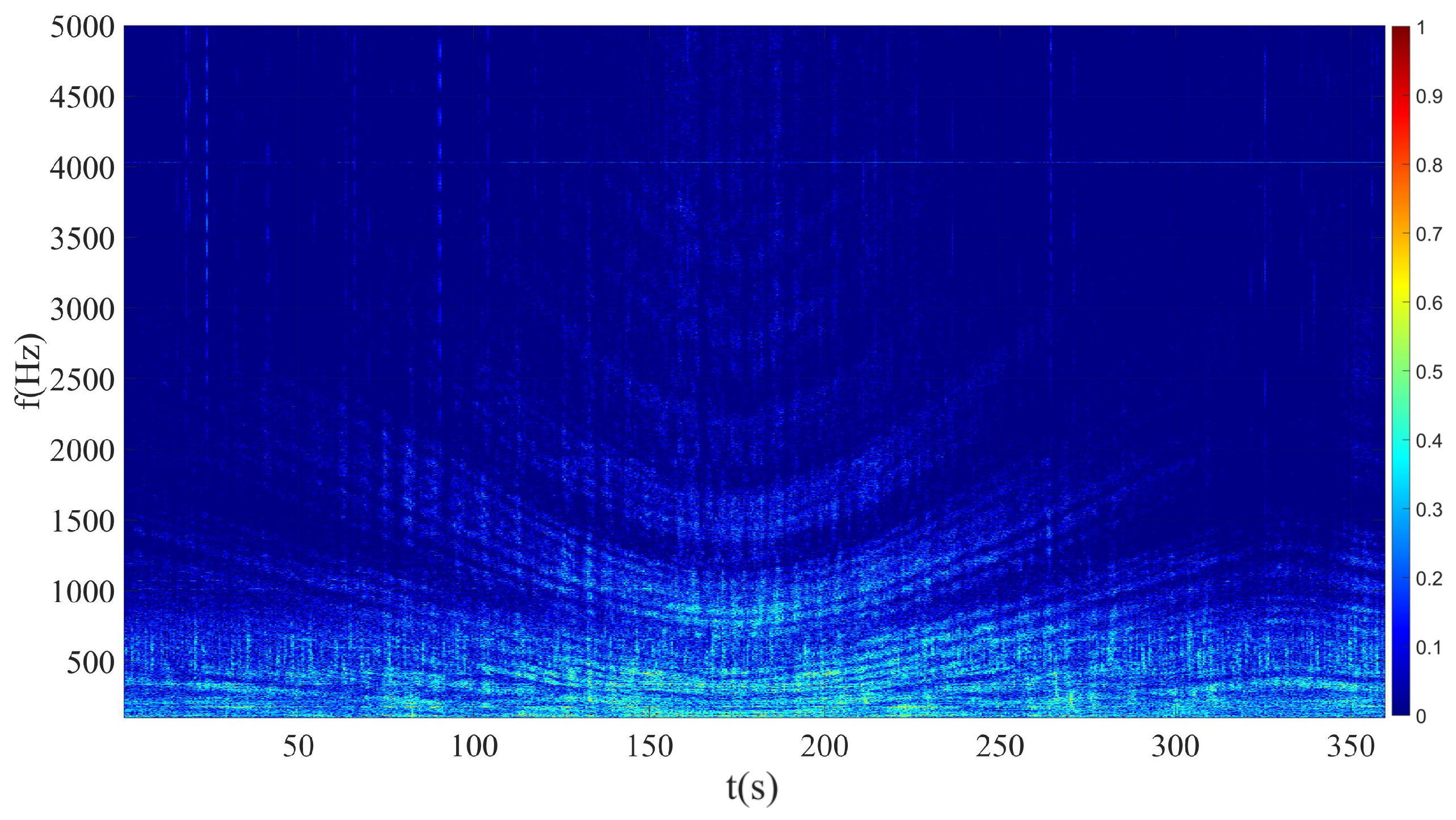
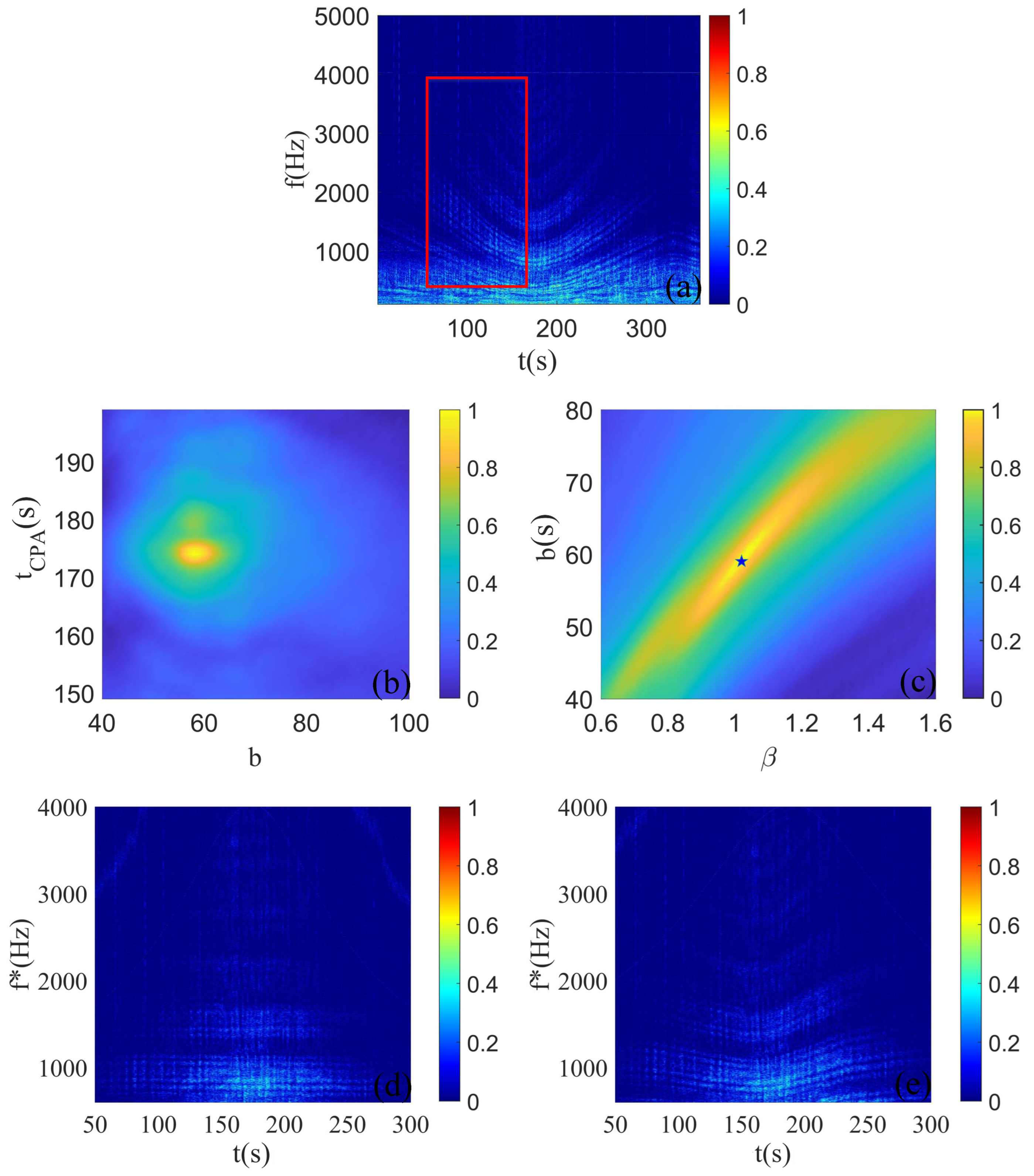
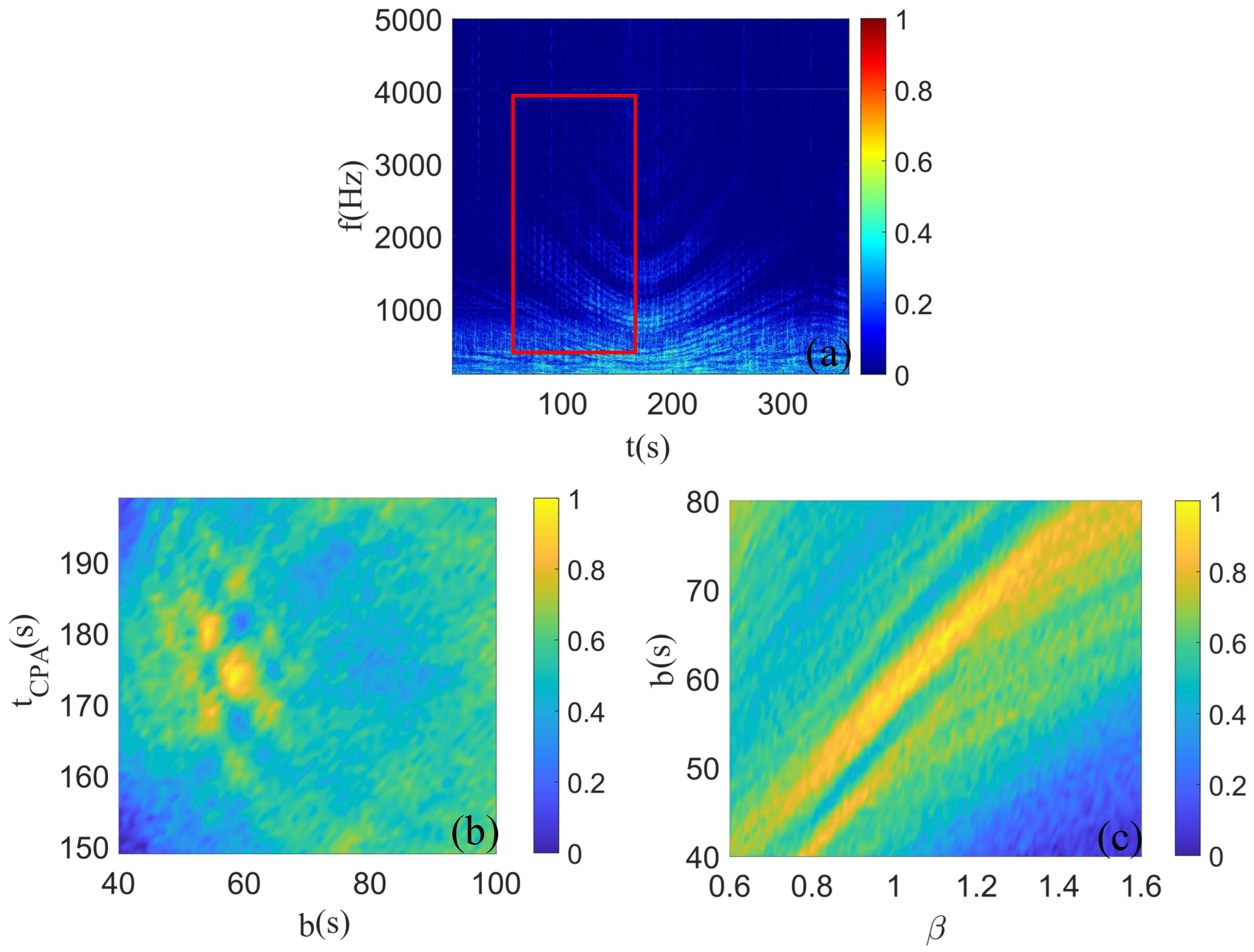
• The received signal is transformed by a short-time Fourier transform to obtain its time–frequency spectrum $I(f,t)$, and the time window $[t_1,t_2]$ and frequency window $[f_1,f_2]$ for parameter estimation are selected in the time–frequency spectrum.
• Define the search grids for parameters b, $t_{CPA}$ and $\beta$, denoted by $\{b_1,b_2,\dots ,b_M\}$, $\{t_{CP{A}_1},t_{CP{A}_2},\dots ,t_{CP{A}_N}\}$ and $\{{\beta }_1,{\beta }_2,\dots ,{\beta }_Q\}$.
• Select any parameter $\{b_m,t_{CP{A}_n},{\beta }_q\}(b_m\in \{b_1,b_2,\dots ,b_M\}$, $t_{CP{A}_n}\in \{t_{CP{A}_1},t_{CP{A}_2},\dots ,t_{CP{A}_N}\},{\beta }_q\in \{{\beta }_1,{\beta }_2,\dots ,{\beta }_Q\})$. The Hyperbola-warping transform is applied to the sound intensity in the $t\in [t_1,t_2]$ range to obtain $I_R(f,t,b_m,t_{CPAn},{\beta }_q)$.
• Calculate the average value of $I_R(f,t,b_m,t_{CPAn},{\beta }_q)$ over the time window, denoted as ${\overline{I}}_R(f,b_m,t_{CPAn},{\beta }_q)$

  $${\overline{I}}_R(f,b_m,t_{CPAn},{\beta }_q)={\displaystyle \frac{1}{t_2-t_1}}\underset{t_1}{\overset{t_2}{\int }}{I}_R(f,t,b_m,t_{CPAn},{\beta }_q)dt$$

  (13)
• Calculate the spectrum of ${\overline{I}}_R(f,b_m,t_{CPAn},{\beta }_q)$, denoted as $Y(\Omega ,b_m,t_{CPAn},{\beta }_q)$.
• Define the standard deviation of the cost function as $Y(\Omega ,$$b_m,t_{CPAn},{\beta }_q)$, denoted by $L(b_m,t_{CP{A}_n},{\beta }_q)$.

  $$\begin{array}{cccc}\hfill & \hfill & \hfill L(b_m,t_{CP{A}_n},{\beta }_q)=\sigma \left(Y(\Omega ,b_m,t_{CPAn},{\beta }_q)\right)& \hfill \end{array}$$

  (14)
• Repeat steps 3–6 until all parameter combinations in the search grid are traversed. When the cost function $L(b_m,t_{CP{A}_n},{\beta }_q)$ reaches the maximum value, the corresponding parameter combination is the estimated motion parameter, denoted by $\{\widehat{b},{\widehat{t}}_{CPA},\widehat{\beta }\}$.

  $$\begin{array}{cccc}\hfill & \hfill & \hfill \{\widehat{b},{\widehat{t}}_{CPA},\widehat{\beta }\}=\underset{{\mathrm{b}}_{\mathrm{m}},{\mathrm{t}}_{\mathrm{CPAn}},{\beta }_{\mathrm{q}}}{\mathrm{argmax}}(L(b_m,t_{CPAn},{\beta }_q\left)\right)& \hfill \end{array}$$

  (15)

3. Simulation

The simulation is conducted in a basic shallow-water, range-independent waveguide environment, the sound speed in the water column is $c_w=1500$ m/s, the water depth is 40 m, parameters of the bottom are $c_b=1593$ m/s, ${\rho }_b=1.76$ g/cc, ${\alpha }_b=0.2$ dB/km/Hz. A target, positioned at a depth z of 2 m, navigates at a velocity of 5 m/s along the path depicted in Figure 1. A hydrophone, situated at a depth $z_s$ of 7 m, remains in a fixed location. The time of the closest point of approach ($t_{CPA}$) between the hydrophone and the target is recorded as 500 s, with the corresponding nearest distance ($r_{CPA}$) being 500 m. The distance r between the hydrophone and the target is illustrated as the black line in Figure 7a. The normal mode model, Kraken, is utilized to compute the sound field between 200 s to 400 s (represented by the red line in Figure 7a), for parameter estimation, as shown in Figure 7b.

According to the theoretical framework detailed in Section 2, the ambiguity map of the cost function L is presented in Figure 7c,d. The parameters corresponding to the peak value of the ambiguity map are $b=101$ s, $t_{CPA}=500$ s, $\beta =0.95$, and the real parameters are $b=100$ s, $t_{CPA}=500$ s, $\beta =1$. To demonstrate the algorithm’s processing capability in the time–frequency domain on full-plane interference fringes, the time–frequency spectrum is transformed using the peak estimated parameters ($b=101$ s, $t_{CPA}=500$ s, $\beta =0.95$), as depicted in Figure 8a. Each bright (dark) stripe in the image is a straight line. The error parameters ($b=125$ s, $t_{CPA}=470$ s, $\beta =1$) are selected to transform the time–frequency spectrum, as shown in Figure 8b.

In contrast to Figure 8a,b, the algorithm presented in this paper takes into account the contributions of all interference fringes in the time–frequency domain to the analysis results.

As reported in Reference [21], the Hough transform can estimate parameters b, $t_{CPA}$ and $\beta$, but it is designed to process individual interference fringes within the time–frequency domain.

To verify the anti-interference performance of the algorithm, we add white noise to the time–frequency spectrum diagram shown in Figure 7b according to Equation (16), so that $SNR=10$ dB, as shown in Figure 9a. In this figure, the red dashed line represents the interference fringe selected by the Hough transform.

$$SNR=10\ast {log}_{10}^{(Ps/Pn)}$$

(16)

where $P_s$ represents the average power of the signal and $P_n$ represents the average power of the noise.

Analyzing the processing results of the two algorithms in Figure 9, at a signal-to-noise ratio (SNR) of 10 dB, the peak of the Hough transform is located at $b=111$ s, $t_{CPA}=505$ s, $\beta =0.9$; whereas the peak of the full-plane Hyperbola-warping transform is at $b=104$ s, $t_{CPA}=501$ s, $\beta =0.96$, with the actual values being $b=100$ s, $t_{CPA}=500$ s, $\beta =1$. Comparing the outcomes, the conventional Hough transform can essentially predict the target parameters at this SNR, but since it processes a single stripe in the time–frequency spectrum, the parameter estimation results are subject to false peak interference, leading to relatively higher errors, as depicted in Figure 9b,c. The full-plane Hyperbola-warping transform proposed in this paper considers the contributions of all interference fringes in the time–frequency domain, therefore achieving superior parameter estimation results, as shown in Figure 9d,e.

To verify the performance of the two algorithms under different SNRs, white noise with different SNRs is added to the time–frequency spectrum of Figure 7b. The proposed algorithm and the conventional Hough transform are applied to time–frequency spectrums under varying signal-to-noise ratios, with the estimation results for three parameters presented in Figure 10a–c. It can be observed from these figures that the conventional Hough transform exhibits significant estimation errors for all three parameters when the SNR is below 6 dB. Even at SNRs of 6 dB and above, the estimation results from the Hough transform show considerable fluctuations due to noise interference. In contrast, the proposed algorithm, which takes into account the contributions of all interference fringes in the time–frequency domain, is capable of estimating parameters even at SNRs as low as −4 dB. This demonstrates approximately a 10 dB improvement in noise resistance compared to the conventional Hough transform. Moreover, at higher SNRs, the parameter estimation results from the proposed algorithm are more stable.

4. Results of Sea Trial Experiments

The sea trial data come from the single hydrophone target observation experiment carried out by the Acoustic Laboratory of Ocean University of China in Qingdao offshore in June 2022. The experiment took place near Xiaogong Island in the vicinity of Qingdao, where the water depth was approximately 24 m, as shown in Figure 11a. The position of the hydrophone is marked with a red circle in Figure 11a, and the sound velocity profile is shown in Figure 11b.

The hydrophone used in the experiment is a self-contained hydrophone with a sensitivity of −180 dB re 1V/μPa. It is fixed on the buoy and has a depth of about 5 m, as shown in Figure 11c. The target vessel is a 150-horsepower fishing boat, depicted in Figure 11d. The vessel’s trajectory and the buoy’s position are detailed in Figure 12a, with the distance between them illustrated in Figure 12b. The nearest distance $r_{CPA}$ is 233.33 m, and the nearest point time $t_{CPA}$ is 175 s.

According to the data of hand-held GPS, the moving speed of the target ship is drawn as shown in Figure 12c, and the average speed $\overline{v}$ between 90 s and 300 s is 4.1301 m/s. If we take the average speed $\overline{v}$ of the target in this period as the speed of the target, the real parameter $b=r_{CPA}/v$$=233.33/4.1301=56.495$ (s) of the target can be inferred.

Figure 13 shows the time–frequency diagram of the noise signal received by the target during the trajectory navigation shown in Figure 12a. It can be seen from the figure that the overall shape of the interference fringes is hyperbolic, which is consistent with the simulation results, but the signal-to-noise ratio of the overall signal is relatively low. From the frequency domain axis, the more obvious interference fringes are concentrated in the frequency range of $[600,4000]$ Hz. The frequency band less than 600 Hz is seriously disturbed by background noise. From the time axis, in the time period of $[50,300]$ S, the interference fringes are more obvious.

Therefore, for parameter estimation, we select the time segment from 50 s to 150 s and the frequency band from 600 Hz to 4000 Hz, as indicated in the red box of Figure 14a. Utilizing the algorithm detailed in Section 2, the cost function for parameter estimation is derived and displayed in Figure 14b,c. The parameter estimates corresponding to the peak of the ambiguity map are: $b=58$ s, $t_{CPA}=175$ s, $\beta =0.95$, which are basically consistent with the real parameters($b=56.495$ s, $t_{CPA}=175$ s, $\beta =1.02$).

To show the processing ability of the algorithm for interference fringes more vividly, we set the parameter as the peak value of the cost function ($b=58$ s, $t_{CPA}=175$ s, $\beta =0.95$). The converted time–frequency spectrum is shown in Figure 14d. The interference fringes in the figure become straight lines. When the parameter is set to the error value ($b=80$ s, $t_{CPA}=190$ s, $\beta =0.9$), the converted time–frequency spectrum is shown in Figure 14e. The interference fringes in the figure show irregular bending.

To compare the processing capabilities of the traditional Hough transform and the full-plane Hyperbola-warping transform proposed in this paper on actual sea trial data, we selected signals from the same time segments for Hough transform processing, as shown in Figure 15a. The resulting parameter estimation is depicted in Figure 15b,c, with peaks located at $b=58$ s, $t_{CPA}=173$ s, $\beta =1.06$, which are close to the true parameters ($b=56.495$ s, $t_{CPA}=175$ s, $\beta =1.02$). However, the parameter estimation contains many false peaks, making the results less distinct.

To further compare the processing effects of the traditional Warping transform and the full-plane Hyperbola-warping transform on actual data, we set the frequency band to [600, 4000] Hz and selected time periods ranging from [5, 105] s to [180, 280] s, performing estimations at every 5 s interval. The comparative results for the three parameters are displayed in Figure 16a–c.

To quantify the estimation capability of the two algorithms for the three parameters, an increase in detection distance D is introduced as a metric for their detection ability, as shown in Equation (17).

$$D={\displaystyle \frac{\left|t_{CPA}-t_W\right|}{\left|t_{CPA}-t_H\right|}}-1$$

(17)

where $t_H$ denotes the time when the Hough transform approaches the true value, and $t_W$ indicates the time when the algorithm presented in this paper approaches the true value.

Analyzing Figure 16a for the estimation of the parameter $t_{CPA}$, the conventional Hough transform begins to approach the true value at 50 s, stabilizing around the true value around 90 s, whereas the algorithm proposed in this paper starts to approach the true value at 25 s and stabilizes around the true value by 50 s, resulting in an increase in detection distance D by 47%. Analyzing Figure 16b for the estimation of the parameter b, the traditional Hough transform approaches the true value at 50 s, while the proposed algorithm approaches the true value at 25 s, resulting in an increase in detection distance D by 20%. Analyzing Figure 16c for the estimation of the parameter $\beta$, the conventional Hough transform begins to approach the true value at 50 s with significant estimation errors, whereas the algorithm presented in this paper starts to approach the true value at 25 s and substantially reduces the estimation errors, resulting in an increase in detection distance D by 20%.

Considering the estimation results of the three parameters, the algorithm proposed in this paper demonstrates better stability, smaller estimation errors, and at least a 20% increase in detection distance compared to the conventional Hough transform.

5. Discussion and Concluding Remarks

In this paper, we introduce a novel single hydrophone target parameter estimation method that utilizes the Hyperbola-warping transform. It can estimate the motion parameters of the target: $t_{CPA}$, $b=r_{CPA}/v$ and $\beta$ before the target reaches the nearest point when only the time–frequency spectrum of the partial target is known. Unlike conventional methods (Hough transform), our approach takes into account the contributions of all interference fringes in the time–frequency domain, leading to improved accuracy and significantly enhanced noise resistance.

In simulation experiments, the proposed method demonstrated approximately 10 dB superior anti-noise performance compared to the traditional Hough transform. Furthermore, during sea trial experiments, our method was able to predict the target parameters with a detection range improvement of 20% and with greater stability than the Hough transform. These results substantiate the proposed algorithm’s enhanced anti-noise capabilities and stable parameter estimation abilities.

However, this study focuses solely on range-independent waveguide environments. The effectiveness of the algorithm in range-dependent waveguide environments warrants investigation in future research.

References

1. Thode, A.M.; Kuperman, W.; D’Spain, G.; Hodgkiss, W. Localization using Bartlett matched-field processor sidelobes. J. Acoust. Soc. Am. 2000, 107, 278–286. [Google Scholar] [CrossRef]
2. Thode, A.M. Source ranging with minimal environmental information using a virtual receiver and waveguide invariant theory. J. Acoust. Soc. Am. 2000, 108, 1582–1594. [Google Scholar] [CrossRef]
3. Heaney, K.D. Rapid geoacoustic characterization using a surface ship of opportunity. IEEE J. Ocean. Eng. 2004, 29, 88–99. [Google Scholar] [CrossRef]
4. Heaney, K.D. Rapid geoacoustic characterization: Applied to range-dependent environments. IEEE J. Ocean. Eng. 2004, 29, 43–50. [Google Scholar] [CrossRef]
5. Li, P.; Wu, Y.; Guo, W.; Cao, C.; Ma, Y.; Li, L.; Leng, H.; Zhou, A.; Song, J. Striation-based beamforming with two-dimensional filtering for suppressing tonal interference. J. Mar. Sci. Eng. 2023, 11, 2117. [Google Scholar] [CrossRef]
6. Song, W.; Gao, D.; Li, X.; Kang, D.; Li, Y. Waveguide invariant in a gradual range-and azimuth-varying waveguide. JASA Express Lett. 2022, 2, 056002. [Google Scholar] [CrossRef]
7. Song, H.; Byun, G. Localization of a distant ship using a guide ship and a vertical array. J. Acoust. Soc. Am. 2021, 149, 2173–2178. [Google Scholar] [CrossRef]
8. Carter, G. Time delay estimation for passive sonar signal processing. IEEE Trans. Acoust. Speech Signal Process. 1981, 29, 463–470. [Google Scholar] [CrossRef]
9. Wu, Q.; Xu, Y. A Nonlinear Data-Driven Towed Array Shape Estimation Method Using Passive Underwater Acoustic Data. Remote Sens. 2022, 14, 304. [Google Scholar] [CrossRef]
10. Zhang, W.; Jiang, P.; Lin, J.; Sun, J. Array shape calibration based on coherence of noise radiated by non-cooperative ships. Ocean Eng. 2024, 303, 117792. [Google Scholar] [CrossRef]
11. Nardone, S.; Lindgren, A.; Gong, K. Fundamental properties and performance of conventional bearings-only target motion analysis. IEEE Trans. Autom. Control 1984, 29, 775–787. [Google Scholar] [CrossRef]
12. Lowney, M.P.; Bar-Shalom, Y.; Luginbuhl, T.; Willett, P. Estimation of the Target State with Passive Measurements and Prior Range Information. In Proceedings of the OCEANS 2023-MTS/IEEE US Gulf Coast, Biloxi, MS, USA, 25–28 September 2023; IEEE: New York, NY, USA, 2023; pp. 1–7. [Google Scholar]
13. Hinich, M.J. Maximum-likelihood signal processing for a vertical array. J. Acoust. Soc. Am. 1973, 54, 499–503. [Google Scholar] [CrossRef]
14. Zhang, X.; Yang, P.; Wang, Y.; Shen, W.; Yang, J.; Wang, J.; Ye, K.; Zhou, M.; Sun, H. A novel multireceiver sas rd processor. IEEE Trans. Geosci. Remote Sens. 2024, 62, 4203611. [Google Scholar] [CrossRef]
15. Zhang, X.; Yang, P.; Wang, Y.; Shen, W.; Yang, J.; Ye, K.; Zhou, M.; Sun, H. LBF-based CS algorithm for multireceiver SAS. IEEE Geosci. Remote Sens. Lett. 2024, 21, 1502505. [Google Scholar] [CrossRef]
16. Wang, C.; Ma, S.; Meng, Z. Array Invariant-Based Source Localization in Deep Sea by Vertical Linear Array. In Proceedings of the 2019 IEEE 2nd International Conference on Information Communication and Signal Processing (ICICSP), Weihai, China, 28–30 September 2019; IEEE: New York, NY, USA, 2019; pp. 180–184. [Google Scholar]
17. Byun, G.; Song, H. Adaptive array invariant. J. Acoust. Soc. Am. 2020, 148, 925–933. [Google Scholar] [CrossRef]
18. Wang, Y.; Chi, C.; Li, Y.; Ju, D.; Huang, H. Passive Array-Invariant-Based Localization for a Small Horizontal Array Using Two-Dimensional Deconvolution. Appl. Sci. 2022, 12, 9356. [Google Scholar] [CrossRef]
19. Lee, S.; Makris, N.C. The array invariant. J. Acoust. Soc. Am. 2006, 119, 336–351. [Google Scholar] [CrossRef] [PubMed]
20. Tao, H.; Hickman, G.; Krolik, J.L.; Kemp, M. Single hydrophone passive localization of transiting acoustic sources. In Proceedings of the OCEANS 2007-Europe, Aberdeen, UK, 18–21 June 2007; IEEE: New York, NY, USA, 2007; pp. 1–3. [Google Scholar]
21. Turgut, A.; Orr, M.; Rouseff, D. Broadband source localization using horizontal-beam acoustic intensity striations. J. Acoust. Soc. Am. 2010, 127, 73–83. [Google Scholar] [CrossRef] [PubMed]
22. Zhao, C.; Liang, G.; Wang, J.; Qiu, L.; Liu, G.; Dong, W. Single-hydrophone-based passive localization for vertically moving targets in shallow water. Ocean Eng. 2024, 306, 118062. [Google Scholar] [CrossRef]
23. Baraniuk, R.G.; Jones, D.L. Unitary equivalence: A new twist on signal processing. IEEE Trans. Signal Process. 1995, 43, 2269–2282. [Google Scholar] [CrossRef]
24. Bonnel, J.; Thode, A.; Wright, D.; Chapman, R. Nonlinear time-warping made simple: A step-by-step tutorial on underwater acoustic modal separation with a single hydrophone. J. Acoust. Soc. Am. 2020, 147, 1897–1926. [Google Scholar] [CrossRef]
25. Qi, Y.B.; Zhou, S.H.; Zhang, R.H.; Zhang, B.; Ren, Y. Modal characteristic frequency in a range-dependent shallow-water waveguide and its application to passive source range estimation. Acta Phys. Sin. 2014, 63, 044303. [Google Scholar] [CrossRef]
26. Bonnel, J.; Dosso, S.E.; Ross Chapman, N. Bayesian geoacoustic inversion of single hydrophone light bulb data using warping dispersion analysis. J. Acoust. Soc. Am. 2013, 134, 120–130. [Google Scholar] [CrossRef] [PubMed]
27. Niu, H.Q.; Zhang, R.H.; Li, Z.L.; Guo, Y.G.; He, L. Bubble pulse cancelation in the time-frequency domain using warping operators. Chin. Phys. Lett. 2013, 30, 084301. [Google Scholar] [CrossRef]
28. Mao, J.; Peng, Z.; Zhang, B.; Wang, T.; Zhai, Z.; Hu, C.; Wang, Q. An Underwater Localization Algorithm for Airborne Moving Sound Sources Using Doppler Warping Transform. J. Mar. Sci. Eng. 2024, 12, 708. [Google Scholar] [CrossRef]
29. Li, X.; Piao, S.; Zhang, H. Modified Warping transformation for typical waveguide with semi-infinite seabed. Harbin Gongcheng Daxue Xuebao/J. Harbin Eng. 2018, 39, 1257–1263. [Google Scholar]
30. Wang, D.; Guo, L.-H.; Liu, J.-J.; Qi, Y.-B. Passive impulsive source range estimation based on warping operator in shallow water. Acta Phys. Sin. 2016, 65, 104302. [Google Scholar] [CrossRef]
31. Brekhovskikh, L.M.; Lysanov, Y.P. Fundamentals of Ocean Acoustics; Springer Science & Business Media: Berlin/Heidelberg, Germany, 2003. [Google Scholar]
32. Chuprov, S.; Brekhovskikh, L. Interference structure of a sound field in a layered ocean. Ocean Acoust. Curr. State 1982, 71–91. [Google Scholar]
33. Porter, M.B. The KRAKEN Normal Mode Program; Naval Research Lab: Washington, DC, USA, 1992. [Google Scholar]
Figure 1. Geometric model of target navigation.
Remotesensing 16 03307 g001
Figure 2. Time–frequency plane interference fringes of sound intensity.
Remotesensing 16 03307 g002
Figure 3. (a) Simulation parameters. (b) Distance between the hydrophone and the target. (c) Time–frequency spectrum of the signal received by the hydrophone.
Remotesensing 16 03307 g003
Figure 4. (a) The selected part of the time–frequency spectrogram. (b) The resampling results of the time–frequency spectrogram using the correct motion parameters. (c) The resampling results of the time–frequency spectrogram using the wrong motion parameters.
Remotesensing 16 03307 g004
Figure 5. (a) When the parameters are correct, the comparison results of I ¯ R ( f ) and I ( f , t C P A ) are obtained. (b) When the parameters are wrong, the comparison results of I ¯ R ( f ) and I ( f , t C P A ) are obtained.
Remotesensing 16 03307 g005
Figure 6. The spectrum analysis results of I ¯ R ( f ) when the parameters are correct and wrong, respectively.
Remotesensing 16 03307 g006
Figure 7. (a) The black line represents the distance between the hydrophone and the target throughout the entire time period, while the red line indicates the distance between the hydrophone and the target during the selected time segment. (b) Time–frequency spectrum of the signal received by the hydrophone. (c,d) Ambiguity map of motion parameter search.
Remotesensing 16 03307 g007
Figure 8. (a) The time–frequency spectrum when the parameter takes the peak value ( b = 101 s, t C P A = 500 s, β = 0.95 ) of the cost function. (b) The time–frequency spectrum when the parameter takes the wrong value ( b = 125 s, t C P A = 470 s, β = 1 ).
Remotesensing 16 03307 g008
Figure 9. (a) Add Gaussian white noise with SNR = 10 dB in Figure 7b, where the red line represents the fringe selected by the Hough transform. (b,c) are the parameter estimation results of the Hough transform. (d,e) are the parameter estimation results of the full-plane Hyperbola-warping transform.
Remotesensing 16 03307 g009
Figure 10. (ac) present comparisons between the estimated target parameters at various SNRs and their corresponding true values.
Remotesensing 16 03307 g010
Figure 11. (a) Nautical chart of the experimental area, where the purple dashed line represents the shipping route. (b) The sound velocity profile. (c) Physical map of the buoy. (d) Physical map of the fishing boat used in the experiment (target ship).
Remotesensing 16 03307 g011
Figure 12. (a) The target trajectory and buoy position. (b) The black line indicates the distance between the target and the buoy throughout the entire time period, while the red line represents the distance during the selected time segment. (c) The target navigation speed.
Remotesensing 16 03307 g012
Figure 13. Time–frequency diagram of buoy receiving target ship radiated noise.
Remotesensing 16 03307 g013
Figure 14. (a) Time–frequency diagram of a buoy receiving target ship radiated noise, where the red square indicates the selected time segment and frequency band. (b,c) are the parameter estimation results of the full-plane Hyperbola-warping transform, where the pentagram indicates the peak values. (d) The time–frequency spectrum when the parameter takes the peak value ( b = 58 s, t C P A = 175 s, β = 0.95 ) of the cost function. (e) The time–frequency spectrum when the parameter takes the wrong value ( b = 80 s, t C P A = 190 s, β = 0.9 ).
Remotesensing 16 03307 g014
Figure 15. (a) The time–frequency spectrum processed by the Hough transform (within the red box). (b,c) are the parameter estimation results of the Warping transform.
Remotesensing 16 03307 g015
Figure 16. (ac) present comparisons between the estimated target parameters at various SNRs and their corresponding true values.
Remotesensing 16 03307 g016
Disclaimer/Publisher’s Note: The statements, opinions and data contained in all publications are solely those of the individual author(s) and contributor(s) and not of MDPI and/or the editor(s). MDPI and/or the editor(s) disclaim responsibility for any injury to people or property resulting from any ideas, methods, instructions or products referred to in the content.