Abstract
This study addresses the potential of machine learning (ML) algorithms in geophysical and geodetic research, particularly for enhancing GNSS time series analysis. We employed XGBoost and Long Short-Term Memory (LSTM) networks to analyze GNSS time series data from the tectonically active Anatolian region. The primary objective was to detect discontinuities associated with seismic events. Using over 13 years of daily data from 15 GNSS stations, our analysis was conducted in two main steps. First, we characterized the signals by identifying linear trends and seasonal variations, achieving values of 0.84 for the XGBoost v.2.1.0 model and 0.81 for the LSTM model. Next, we focused on the residual signals, which are primarily related to tectonic movements. We applied various threshold values and tested different hyperparameters to identify the best-fitting models. We designed a confusion matrix to evaluate and classify the performance of our models. Both XGBoost and LSTM demonstrated robust performance, with XGBoost showing higher true positive rates, indicating its superior ability to detect precise discontinuities. Conversely, LSTM exhibited a lower false positive rate, highlighting its precision in minimizing false alarms. Our findings indicate that the best fitting models for both methods are capable of detecting seismic events (Mw ≥ 4.0) with approximately 85% precision.
1. Introduction
The analysis of time series data is critical in various scientific and engineering areas, particularly in geodesy and geophysics, where it is used to monitor and understand Earth’s dynamic processes. One of the most valuable tools for this purpose is Global Navigation Satellite Systems (GNSS), which provide continuous and precise measurements of the Earth’s surface movements. These measurements are essential for tracking tectonic activities, such as plate motions and deformation, which have significant implications for understanding seismic hazards and geodynamic processes [1]. Although GNSS time series data can comprise further knowledge about the tectonic activity of the region, they also present challenges either due to their general characteristics like noise and/or signal properties [2,3,4,5] or susceptibility to discontinuities caused by seismic events, equipment changes, and environmental factors [6,7,8]. Accurate detection and analysis of these discontinuities are crucial for the reliable interpretation of geophysical phenomena and for maintaining the integrity of GNSS data records.
Traditionally, the analysis of GNSS time series data has relied heavily on conventional statistical and geophysical methods. These methods include linear regression, harmonic analysis, and Kalman filtering, which have been employed to detect trends, periodicities, and abrupt changes in the data. For instance, linear regression is often used to estimate long-term trends, while harmonic analysis is applied to identify periodic signals such as seasonal variations [9]. Kalman filtering, on the other hand, is utilized to smooth the data and to provide real-time estimates of positions and velocities, accommodating both the noise and the dynamic nature of the GNSS measurements [10]. Although these techniques have been instrumental in advancing our understanding of tectonic movements and seismic activities, they often require extensive manual intervention and expert knowledge to accurately interpret the results [11,12]. Additionally, conventional methods can be limited in their ability to handle the nonlinearities and complexities inherent in GNSS time series, particularly when dealing with large datasets or subtle geophysical signals. For example, detecting transient deformation events, such as slow slip events, requires sophisticated modeling techniques and careful examination of the data [6,8,13,14]. As a result, there is a growing recognition of the need for more automated and robust approaches to enhance the accuracy and efficiency of time series analysis in geodesy and geophysics.
Machine learning (ML) algorithms have introduced a paradigm shift in the analysis of GNSS time series data. Machine learning offers powerful tools for modeling complex and nonlinear relationships within large datasets, enabling the detection of patterns and anomalies that may be overlooked by conventional methods. The ability of ML algorithms to learn from data and improve over time makes them particularly well-suited for applications in geodesy and geophysics, where continuous monitoring and real-time analysis are essential. Moreover, machine learning techniques can automate the process of time series analysis, reducing the need for manual intervention and allowing for more efficient data processing [15]. The integration of ML algorithms into geophysical research has the potential to significantly enhance our ability to detect and interpret geophysical phenomena, providing deeper insights into tectonic processes and improving the accuracy of seismic hazard assessments [15,16].
Recent studies have demonstrated the effectiveness of machine learning algorithms in analyzing GNSS time series data for various applications. For example, Wang et al. [17] developed a novel Attention Mechanism with a Long Short-Time Memory Neural Network (AMLSTM NN) model to predict landslide displacement, demonstrating significant potential in accurately forecasting GNSS time series data. Similarly, Crocetti et al. [18] utilized ML techniques for the detection of transient signals in GNSS data, showcasing the robustness of these methods in geophysical monitoring. Some other studies also incorporated many different ML algorithms to analyze GNSS time series for geophysical or geodynamic purposes to test the robustness and possible contributions of these new techniques [19,20,21,22,23,24]. These studies highlight the diverse capabilities of machine learning algorithms in handling the complexities of GNSS time series data, paving the way for more advanced and automated geophysical analysis.
The Anatolian region, situated at the intersection of the Eurasian, African, and Arabian plates, is one of the most seismically active areas in the world [25]. This unique tectonic setting makes it an ideal case study area for GNSS time series analysis. The North Anatolian Fault (NAF) and the East Anatolian Fault (EAF) are the primary tectonic features of this region. The NAF, a right-lateral strike-slip fault extending over 1200 km [26], has been the source of numerous devastating earthquakes, such as the 1999 Izmit and Duzce earthquakes [27]. The EAF, a left-lateral strike-slip fault [28], also accommodates significant tectonic motion and has been associated with major seismic events, i.e., 2011 Van (Mw 7.1), 2017 Kos (Mw 6.6), 2020 Samos earthquake (Mw 6.9), 2020 Elazığ (Mw 6.8) and 2023 Kahramanmaras earthquakes (Mw 7.8) [23,29,30,31,32]. The complex interactions between these fault systems and the Anatolian microplate’s westward escape are driven by the northward convergence of the Arabian plate and the subduction of the African plate beneath the Eurasian plate along the Hellenic and Cyprus trenches [33,34,35].
The high seismic activity and documented fault systems in Anatolia provide a rich dataset for GNSS observations, making it a natural laboratory for studying tectonic processes. Continuous GNSS monitoring in this region has produced extensive time series data, which are crucial for understanding the mechanics of fault interactions, strain accumulation, and release processes. By focusing on Anatolia, researchers can leverage the region’s active tectonic environment to test and refine machine learning algorithms for detecting and interpreting geophysical phenomena. The insights gained from such studies not only enhance our understanding of Anatolian tectonics but also improve our understanding of methods to contribute to seismic hazard assessments and risk mitigation strategies in other tectonically active regions.
The aim of this study is to develop and evaluate the effectiveness of machine learning algorithms for detecting discontinuities in GNSS time series data from the tectonically active region of Anatolia. By leveraging the rich dataset generated by continuous GNSS observations, this study seeks to enhance the accuracy and efficiency of discontinuity detection, which is critical for interpreting tectonic processes and assessing seismic hazards. Specifically, the study will apply and compare the performance of two advanced machine learning techniques, XGBoost and Long Short-Term Memory (LSTM) networks, to identify discontinuities and transient signals within the time series data [36,37]. We will focus on 15 continuous GNSS stations, each providing over 13 years of data, to obtain a comprehensive analysis and robust results. Additionally, we analyze the general characteristics of each time series such as linear trend and seasonal–semi-seasonal periodic signals, training the aforementioned algorithms by designing multiclass structuring methods i.e., [18,19].
Accordingly, Section 2 provides a detailed description of the data collection process, the GNSS stations used in the study, and the acquisition of the raw time series dataset evaluating daily GNSS data. Section 3 includes the implementation details of the XGBoost and LSTM algorithms, and presents our strategies for applying these algorithms to the time series. Section 4 includes a comprehensive analysis of the dataset using the adopted algorithms. We present our best-fitted models for both methods, referring to related parameters and solutions. We analyze the entire signal of each station, particularly focusing on discontinuity detection. We then compare the performance of the machine learning models and discuss our solutions referring to previous studies in Section 5. Finally, Section 6 concludes the study, summarizing the key contributions and suggesting directions for future research. Further details on the methods and a brief summary of the theory behind each employed ML algorithm can be found in Appendix A.
2. Data
2.1. Data Acquiring
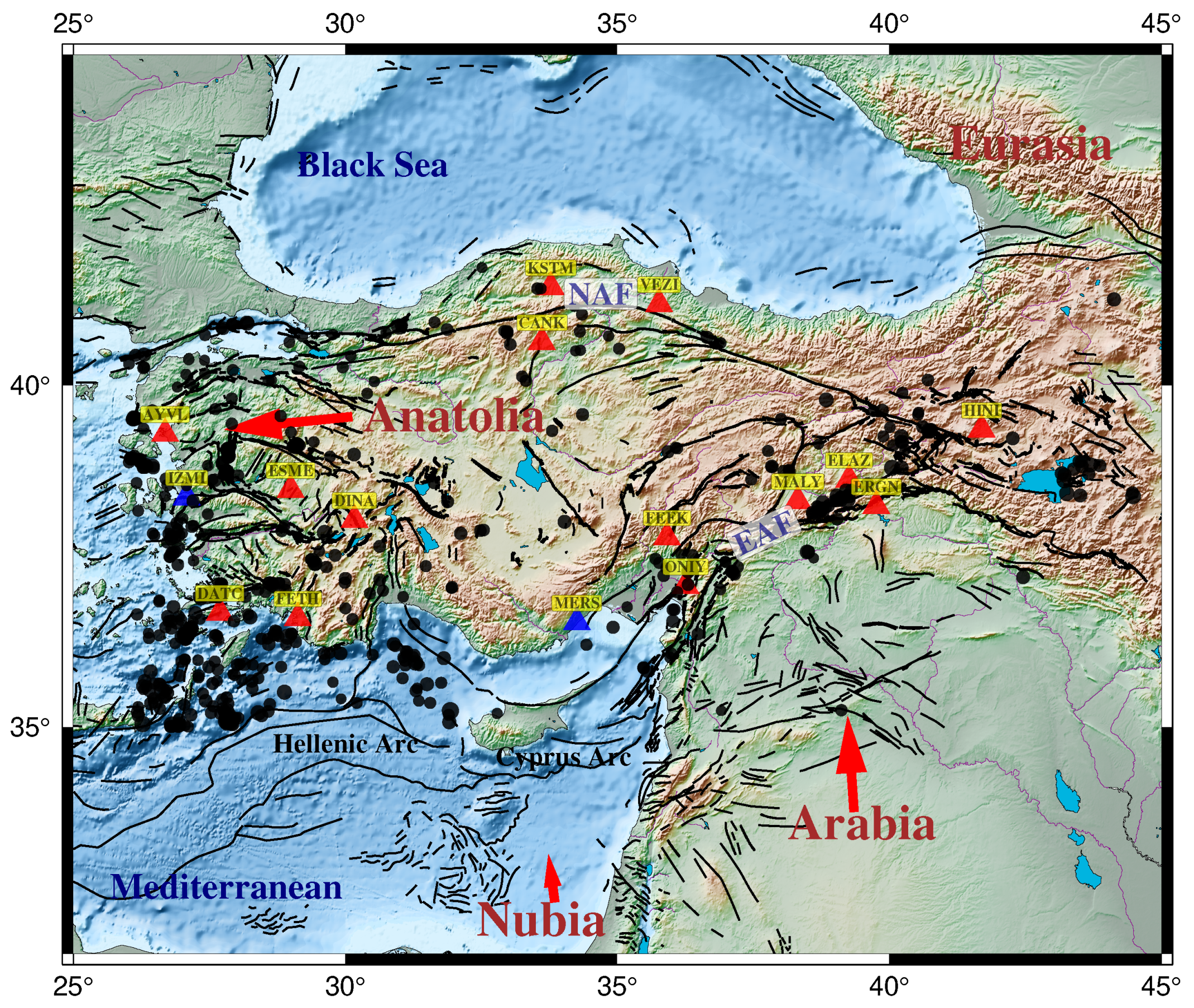
The GNSS time series data utilized in this study were obtained from the Turkish Continuous Permanent GNSS Network (TUSAGA) and the International GNSS Service (IGS). These networks offer continuous observations of Earth’s surface movements, which are crucial for monitoring tectonic activities in the region. The dataset comprises daily coordinate measurements from 15 GNSS stations, each with over 13 years of continuous data (Figure 1).
We applied three criteria to select the GNSS stations: (i) Distance to major earthquakes such as the 2017 Kos, 2019 Samos, and 2020 Elazig events. Our goal was to include stations situated in the near field of these significant seismic events to evaluate the effectiveness of discontinuity detection methods. Additionally, we selected stations that have been previously reported to exhibit coseismic displacements greater than 5 mm due to these major earthquakes, which is crucial for validating the fundamental consistency of our analysis. (ii) The data span of the GNSS stations was another key factor in our selection process. We prioritized stations that met the first criteria and had at least 10 years of continuous data with no more than a 6 month gap. This avoids the possiblity of missing of our semi-annual signal detection, which is essential for detecting seasonal variations in the GNSS time series data. (iii) Lastly, we considered the spatial distribution of seismic activity, as shown in Figure 1. We aimed to select stations located near seismically active regions where earthquakes frequently occurred, according to our catalog. The dataset spans from 1 January 2009, when the Turkish Continuous network began operations, to the end of 2022. Although the IGS stations have a longer data history, we decided to start the same initial epoch for all stations to maintain spatio-temporal consistency among the stations.
Additionally, our earthquake catalog was derived from the Regional Centroid Moment Tensor (RCMT) catalog, as detailed by Pondrelli et al. [38]. Our derived catalog includes datasets for earthquakes with moment magnitudes (Mw 3.5), and we applied a filter so that only the first and second quality solutions were selected for our analysis (the details of the quality classification can be found in the catalog itself).

Figure 1.
Assessed GNSS stations and earthquake distributions. Red triangles belong to the TUSAGA network, whereas blue ones are from the IGS. Black circles are earthquakes, scaled by their magnitudes; Mw ≥ 4.0 occurred between 1 January 2009 and 31 December 2022. Black lines are faults digitized from [39]. Red arrows indicate plate motions. Abbreviations: NAF: North Anatolian Fault, EAF: East Anatolian Fault.
2.2. Evaluation of GNSS Data
To convert the raw GNSS data into precise daily positions, the GAMIT/GLOBK software v10.7 package was used [40]. Since GNSS observations are inherently affected by various sources of noise—such as atmospheric interference, satellite ephemeris errors, and multipath effects—it is crucial to employ an analysis method taking into account all these effects to extract the true tectonic signal from the time series data. We thus chose to analyze our dataset using the GAMIT/GLOBK software v10.7, one of the most established and scientifically validated tools for high-precision GNSS data processing. GAMIT/GLOBK is specifically designed to handle the complexities of GNSS data by applying a series of precise corrections and adjustments. It basically adopts a double-differences approach to determine the coordinates of GNSS stations. GAMIT processes the raw GNSS observations by modeling satellite orbits, atmospheric delays, and Earth orientation parameters. These processes enhance the reliability and accuracy of the generated time series independent from the length of the dataset and location. It incorporates sophisticated algorithms, such as wide-narrow lanes, to resolve phase ambiguities, apply corrections for atmospheric conditions, and generate particular frequency combinations to minimize the impact of errors on the final position estimates. The processing involves several key steps, including data cleaning to remove noise and outliers, cycle slip detection and correction to handle phase discontinuities, and ambiguity resolution to solve integer ambiguity in the carrier phase measurements.
Once the daily evaluation was completed by checking several criteria to ensure the accuracy of the process (see [40]), the processed data were then compiled into time series representing the daily positions of each GNSS station over the 13-year period. In the process of analyzing GNSS time series, it is crucial to account for the common mode error (CME), which refers to the systematic errors that affect multiple stations in a similar manner. These errors can arise from various sources, such as satellite orbits, atmospheric conditions, and signal processing issues. By identifying and mitigating the CME during the raw analysis, we can enhance the accuracy and reliability of the positional data. It is important to note that we consider these common mode errors in our study and remove those effects from all stations before starting the machine learning analysis.
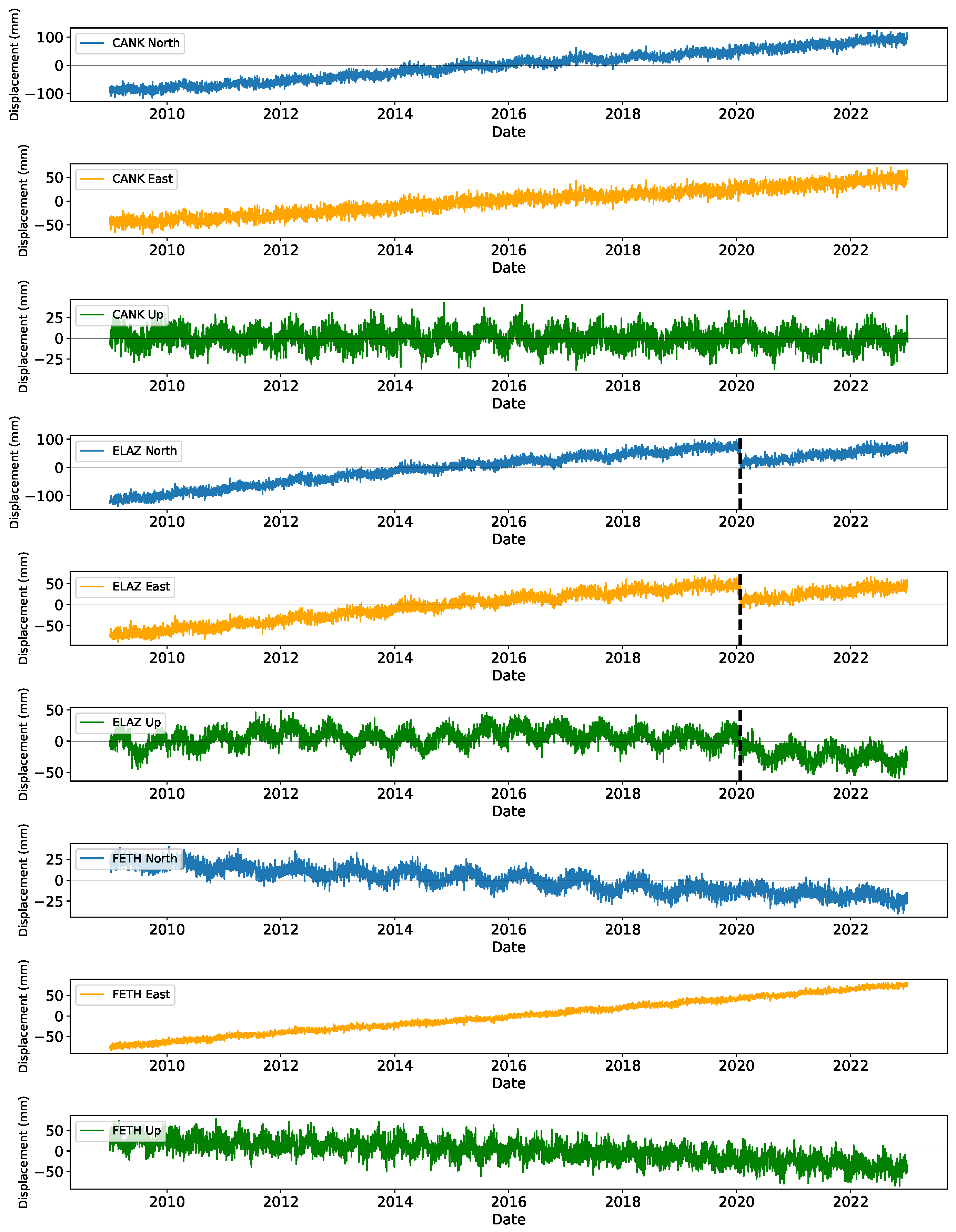
Further details for the daily coordinate processing and time series generation can be found in the study by Herring et al. [40] and the extensive literature therein. Figure 2 shows the raw time series of three stations in our dataset. Additional raw plots are provided in the Supplementary Materials.
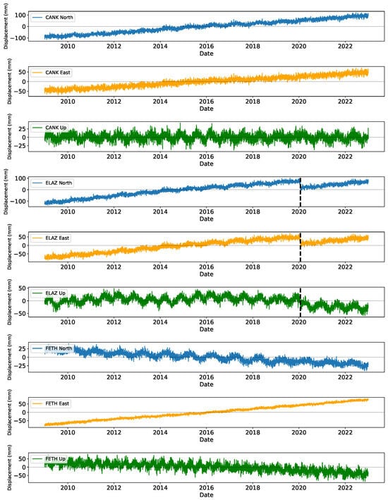
Figure 2.
Raw time series of CANK, ELAZ, and FETH stations, respectively. We chose these stations to show the time series oscillating slowly, being exposed to bigger earthquakes and relatively higher oscillations, respectively. Black dashed lines correspond to the epoch of the Elazig earthquake (Mw 6.9) on the ELAZ time series.
3. Methodology
The dataset was divided into training, validation, and testing sets to achieve robust model evaluation. The training set was used to fit the models, the validation set was utilized to tune hyperparameters, and the testing set was employed to evaluate the final model performance.
3.1. Data Segmentation and Feature Extraction
Data segmentation involves dividing the continuous GNSS time series into smaller, overlapping windows. This technique allows the analysis of short-term patterns and transient events that may not be apparent in the entire dataset. For this study, we used a sliding window approach with a window size of 21 days and an overlap of 10 days. This window size was chosen based on the typical duration of transient geophysical events, such as slow slip events and episodic tremors, and some previous experiments presented in previous studies, i.e., [19]. Each window is treated as an individual sample for the machine learning model. Here, it is important to note that any windows with more than 10% missing data were excluded from the analysis to maintain data integrity.
Feature extraction transforms each segmented window of the GNSS time series into a set of features that detect the essential characteristics of the data. These features include statistical measures, frequency domain characteristics, trend indicators, and displacement metrics. Specifically, for each window, we extract the mean, standard deviation, skewness, and kurtosis to detect the central tendency, dispersion, and shape of the data distribution. We also estimate the Fourier transform coefficients to analyze the periodic components within the time series. To detect trends and changes within each window, we compute the maximum and minimum displacements, as well as the range of displacements, to highlight significant variations in the GNSS coordinates that may indicate discontinuities or transient events (Table 1). These features are essential for training both XGBoost and LSTM models, as they provide comprehensive insights into the data underlying patterns. In general, we adopted the approach presented by Crocetti et al. [18] to design the feature matrix (see their Figure 3 for further detail).

Table 1.
The features extracted from the time series data for each model. These features include statistical measures and patterns that are critical for the models’ ability. They provide a detailed overview of the key characteristics used in the analysis and modeling process.

Figure 3.
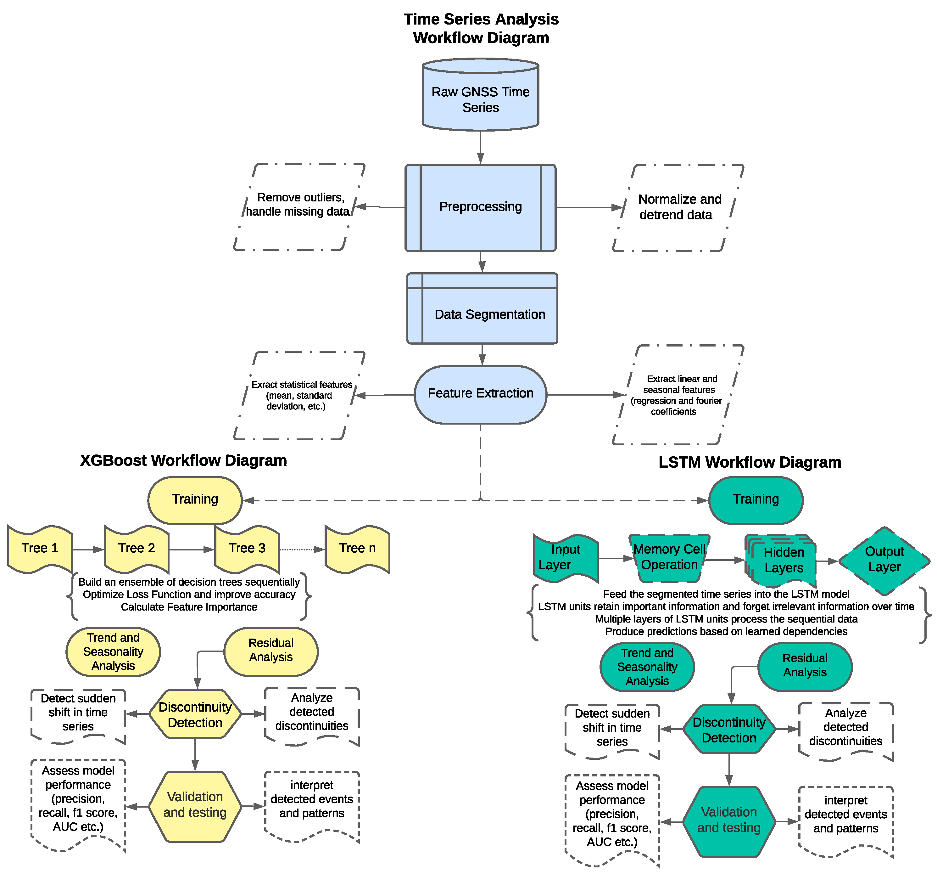
Modeling steps for both XGBoost and LSTM methods. The preprocessing stage was conducted in a similar manner for both of the methods.
3.2. Accuracy and Evaluation Metrics
To investigate the performance of our models, we employ a comprehensive set of metrics that provide a robust evaluation of the models’ predictive capabilities. Here it is important to note that we also construct these models for the data preprocessing part related to removing trends and seasonal signals. We, therefore, used the metric, also known as the coefficient of determination, along with Root Mean Square Error (RMSE) and Mean Absolute Error (MAE). measures the proportion of the variance in the dependent variable that is predictable from the independent variable(s). It provides insight into the model’s ability to explain the variability of the response data. An value close to 1 indicates a model that explains a high proportion of the variance. These are formulated as below where is the actual value, is the predicted value, is the mean of the actual values, and n is the number of observations.
Furthermore, one of the primary goals of this study is analyzing the residual part, mainly focusing on discontinuity detection and assessing how effectively these models identify discontinuities that correspond to significant seismic events, as recorded in earthquake catalogs. We thus construct a confusion matrix that is quite similar to the one presented by Crocetti et al. [18]. The confusion matrix provides a comprehensive overview of the classification performance by displaying the number of true positives (TP), true negatives (TN), false positives (FP), and false negatives (FN) (Table 2). It also helps to identify specific areas where the model may be underperforming. We then maintain following Crocetti et al.’s [18] approach and implement TP′ values accounting for the true detection in terms of the correct window, but it does not correspond to the actual date of the event.

Table 2.
The main features of the confusion matrix, including true positives (TP), false positives (FP), true negatives (TN), and false negatives (FN). These elements are critical for evaluating the performance of the models in classifying seismic events.
Additionally, we utilize some other metrics to address the effectiveness of designed confusion matrix. Precision measures the proportion of true positive predictions among all positive predictions made by the model. It is defined as:
High precision indicates a low false positive rate, meaning that the model does not frequently misclassify nondiscontinuities as discontinuities. Recall, also known as sensitivity or true positive rate, measures the proportion of actual discontinuities correctly identified by the model. It can be formulated as:
High recall indicates that the model successfully identifies most of the actual discontinuities. The F1 score is the harmonic mean of precision and recall, providing a single metric that balances the trade-off between these two measures. The F1 score ranges from 0 to 1, with 1 indicating perfect precision and recall.
The Receiver Operating Characteristic (ROC) curve is a graphical representation of the model’s diagnostic ability, plotting the True Positive Rate (TPR) against the False Positive Rate (FPR) at various threshold settings. The area under the curve (AUC) provides a single value to summarize the model’s performance, with values closer to 1 indicating better performance. The AUC-ROC curve plots the true positive rate (recall) against the false positive rate (FPR) at various threshold settings. The false positive rate is defined as:
The general concept and analyzing strategy of this study are shown for both methods in Figure 3.
4. Results
In this section, we present the results of applying XGBoost and LSTM algorithms to GNSS time series data from 15 continuous stations, covering the period from July 2009 to December 2022. The analysis includes data preprocessing to detect and analyze trends and seasonal variations at each station. We trained both XGBoost and LSTM models, extracting features and setting various hyperparameters. We then discuss the validation process and its key parameters to address the precision of each model. Additionally, we examine the evaluation metrics and the comparative performance of both models.
Once the residual time series is obtained, we assess the performance of the adopted algorithms, particularly in detecting discontinuities. Several threshold values were assigned to determine the best-fitting model according to various metrics. Finally, we discuss the robustness of each model in terms of the objective function and present all related numerical outcomes. It is worthwhile to mention that during this process, we tested many different model parameters and values to determine the best-fitting model. Here, we present our final solutions, particularly focusing on selecting different values for hyperparameters and critical features. We only show the time series of a few stations in the main text; however, the numerical results comprise the results of the entire analysis. Additional outcomes are available in the Supplementary Materials.
4.1. Preprocessing of the Time Series
The preprocessing of GNSS time series data is a critical step to enhance the accuracy and reliability of subsequent analysis. It allows us to isolate the tectonic signals of interest by removing extra patterns and trends that may obscure the underlying geophysical phenomena.
The first step in preprocessing the GNSS time series data is to remove linear trends and seasonal signals. Linear trends can result from various factors, including tectonic plate motions, which manifest as long-term linear displacements. Removing these trends allows us to focus on shorter-term variations and transient events. Seasonal variations, often annual or semi-annual, are common in GNSS time series data and can result from environmental factors such as temperature changes, snow load, and hydrological effects [41]. To construct the models, we began by selecting relevant features from the GNSS time series data that could help in predicting the linear and seasonal components. These features included time indices and any additional external factors that might influence the data. The model was trained using a supervised learning approach and multi-class segmentation (see [18,19]), where the target variable was the GNSS positional data. By optimizing the parameters through cross-validation, we fine-tuned the model to accurately detect the linear trends and periodic signals. The fitted models were then used to predict all these components, which were subsequently subtracted from the original time series to obtain residuals.
Missing data is a common issue in GNSS time series analysis, which can arise due to various reasons such as equipment malfunctions, data transmission errors, or environmental obstructions. To maintain the integrity and continuity of the dataset, it is essential to address these gaps. In this study, we employed linear interpolation to fill the missing data points, which provides a simple yet effective method for estimating the missing values based on the available data. This approach helps maintain the temporal structure of the data while minimizing potential biases introduced by more complex imputation methods. After removing the linear and seasonal trends, the normalization of the time series data to have a mean of zero and a standard deviation of one was performed. This process ensures that the data are on a consistent scale, which is essential for the effective application of machine learning algorithms. Normalization helps to mitigate the effects of varying magnitudes in the data, allowing the algorithms to focus on the underlying patterns rather than the absolute values. Finally, once all these preprocessing stages were applied, we assumed that the residuals primarily contained the tectonic signals and other short-term variations of interest. The combined use of XGBoost and LSTM ensures a comprehensive approach to detrending and denoising the GNSS time series data, providing a cleaner dataset for subsequent analysis.
The training process involves preparing the data, initializing the models with optimal hyperparameters, and executing the training process to minimize the loss and maximize the accuracy. The GNSS time series data were split into three sets: training, validation, and testing. The training set comprises data from July 2009 to December 2018. The validation set covers data from January 2019 to December 2020, and the testing set includes data from January 2021 to December 2022. This split ensures that the models are trained on a substantial portion of the data while storing enough data for validation and testing. Table 3 shows the hyperparameters and initial values for the training process.

Table 3.
Initial hyperparameters for both the XGBoost and LSTM models used in the study. These hyperparameters were selected to optimize the models’ performance in detecting target features.
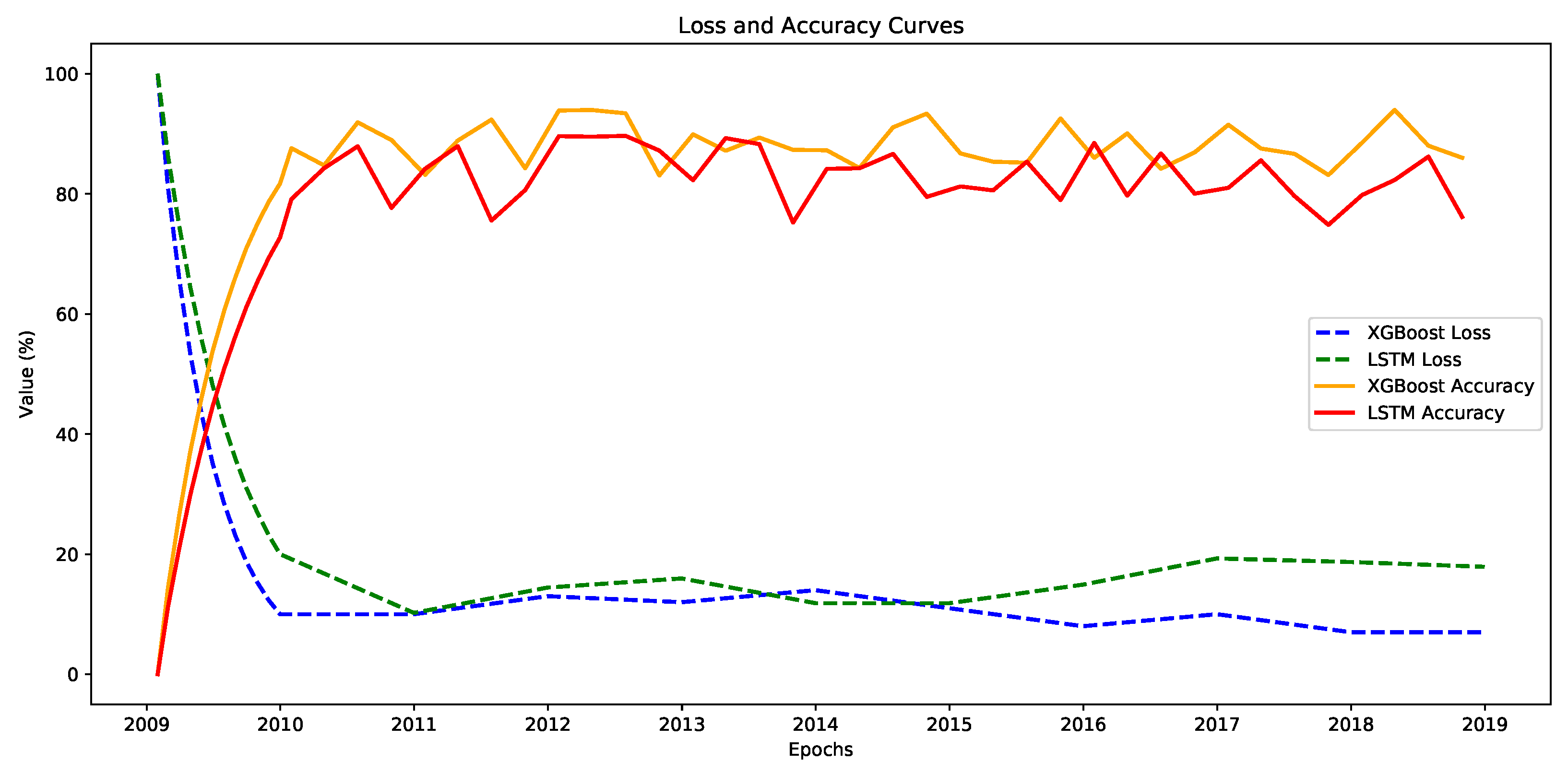
The models were trained using the backpropagation algorithm to minimize the loss function. The training process was monitored using loss and accuracy metrics, with the XGBoost model showing a steady decrease in loss from 25% to 7% and accuracy improvement from 75% to 93%, while the LSTM model saw its loss reduced from 27% to 9% and accuracy increased from 70% to 90% over 50 epochs. The loss and accuracy curves for both models are plotted in Figure 4. The XGBoost model achieved a training loss of 7%, while the LSTM model achieved a training loss of 9%. The training accuracy for the XGBoost model reached 93%, whereas the LSTM model attained a training accuracy of 90%.

Figure 4.
Loss and accuracy curves of each model. The dashed lines represent the training loss curves, while the solid lines represent the accuracy curves. All models show a gradual decrease in loss and a sufficient increase (albeit fluctuate) in accuracy, indicating convergence over time.
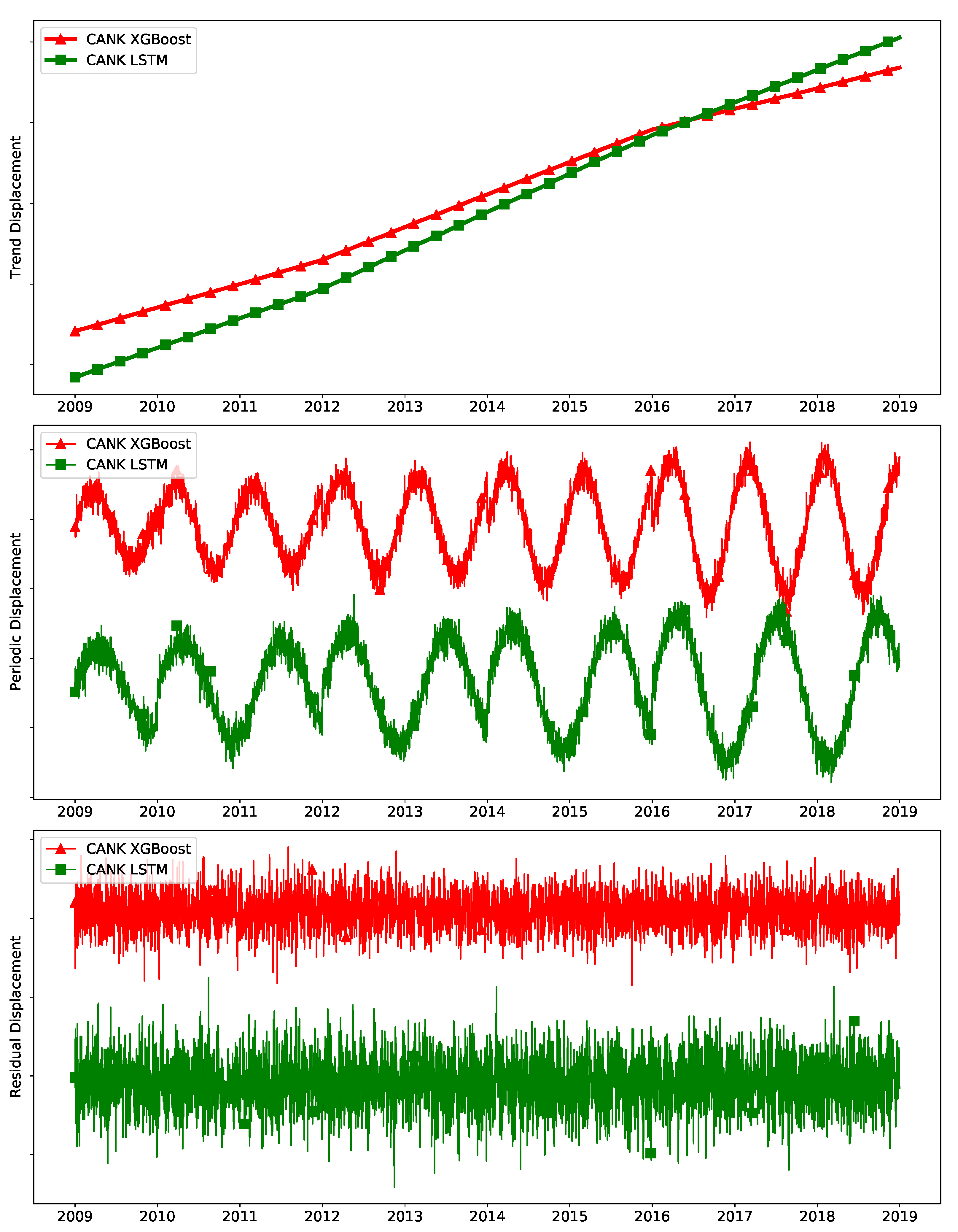
Figure 5 illustrates the time series components utilized for training the XGBoost and LSTM models.
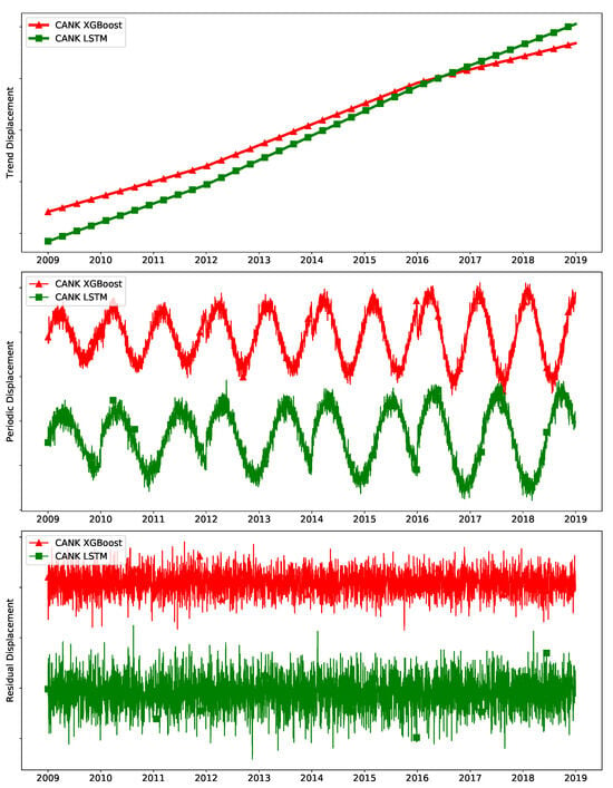
Figure 5.
The training results for each model applied to data from the CANK station. The upper figure displays the extracted trends for each model, highlighting the underlying patterns and long-term changes captured during the training process. The middle figure illustrates the periodic signals identified by each model. This section emphasizes the ability of the models to recognize and represent repeating patterns and seasonal variations in the data. The lower figure presents the residual signal.
The validation process employed 15% of the data as the validation set. The models were assessed on this set to identify the optimal hyperparameters. For the XGBoost model, hyperparameter tuning was conducted using Grid Search, while for the LSTM model, Random Search was adopted as given in Table 4. It seems that there are no strong differences in the results between the initial values of the training process and the tuned hyperparameters. The same values were obtained as best fitted for most of the hyperparameters.

Table 4.
Results of the hyperparameter tuning process for models. It includes all tested values and the final selected values for each parameter. The columns list the names of the parameters, the range of values tested, and the optimal values chosen based on the tuning process.
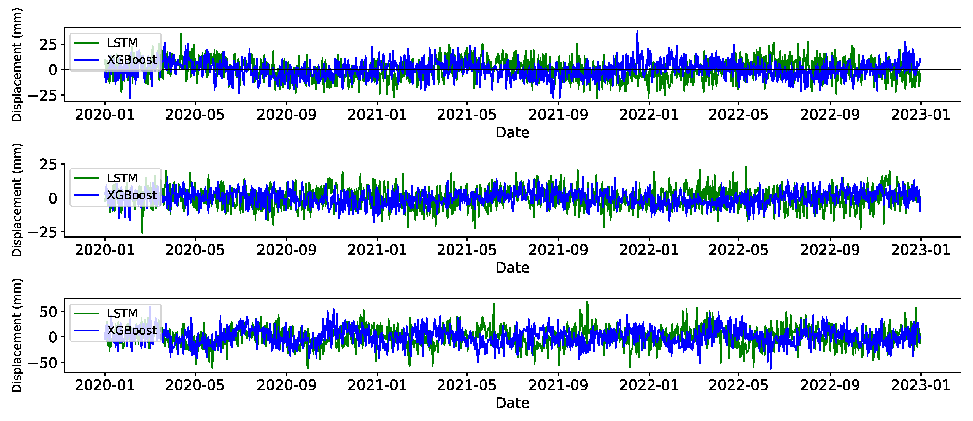
Once the best model and hyperparameters were selected, the final evaluation was performed on the testing set to assess the models’ generalization abilities. The final testing phase utilized the remaining 15% of the data, spanning from January 2021 to December 2022. This evaluation aimed to test the model performances for the “new” data. Comparing the testing results with the validation results revealed consistent performance across both phases, indicating no significant overfitting or underfitting (Figure 6).
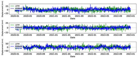
Figure 6.
The prediction results of two models. The blue lines represent the predictions made by the XGBoost model, while the green lines correspond to the predictions made by the LSTM model. Each subplot corresponds to a different station, enabling a comparison of model performance across varied datasets. Notably, the calculated trend values have been removed from the signal, allowing for emphasizing the models’ ability to predict the underlying patterns and variations in the data without the influence of long-term trends.
The XGBoost model achieved a testing MAE of 1.8 mm and RMSE of 2.2 mm, which were closely aligned with the validation MAE of 1.7 mm and RMSE of 2.1 mm, demonstrating consistent predictive accuracy. This consistency implies the model’s robustness and reliability in predicting GNSS time series data for removing trend and seasonal signals. Similarly, the LSTM model’s testing metrics were in alignment with its validation metrics, although slightly lower than those of the XGBoost model.
The results, summarized in Table 5, show that both models achieved values of 0.84 for XGBoost and 0.81 for LSTM, indicating a strong ability to explain 84% and 81% of the variance in the data, respectively. The ability to accurately remove linear trends and seasonal variations from the GNSS time series data is crucial for isolating the tectonic signals of interest. Moreover, the evaluation metrics show the models’ capacity to handle complex, multi-dimensional classified time series data effectively. The consistent performance across training, validation, and testing phases can be interpreted as a contribution to more precisely detecting discontinuities. The model results also indicate the effectiveness of using machine learning techniques for preprocessing GNSS time series to monitor the general characteristic(s) of a long-term time series.

Table 5.
Performance metrics for both models, including Mean Absolute Error (MAE), Root Mean Square Error (RMSE), and R² values. These metrics provide an evaluation of each model’s accuracy and predictive capability.
4.2. Residual Analysis
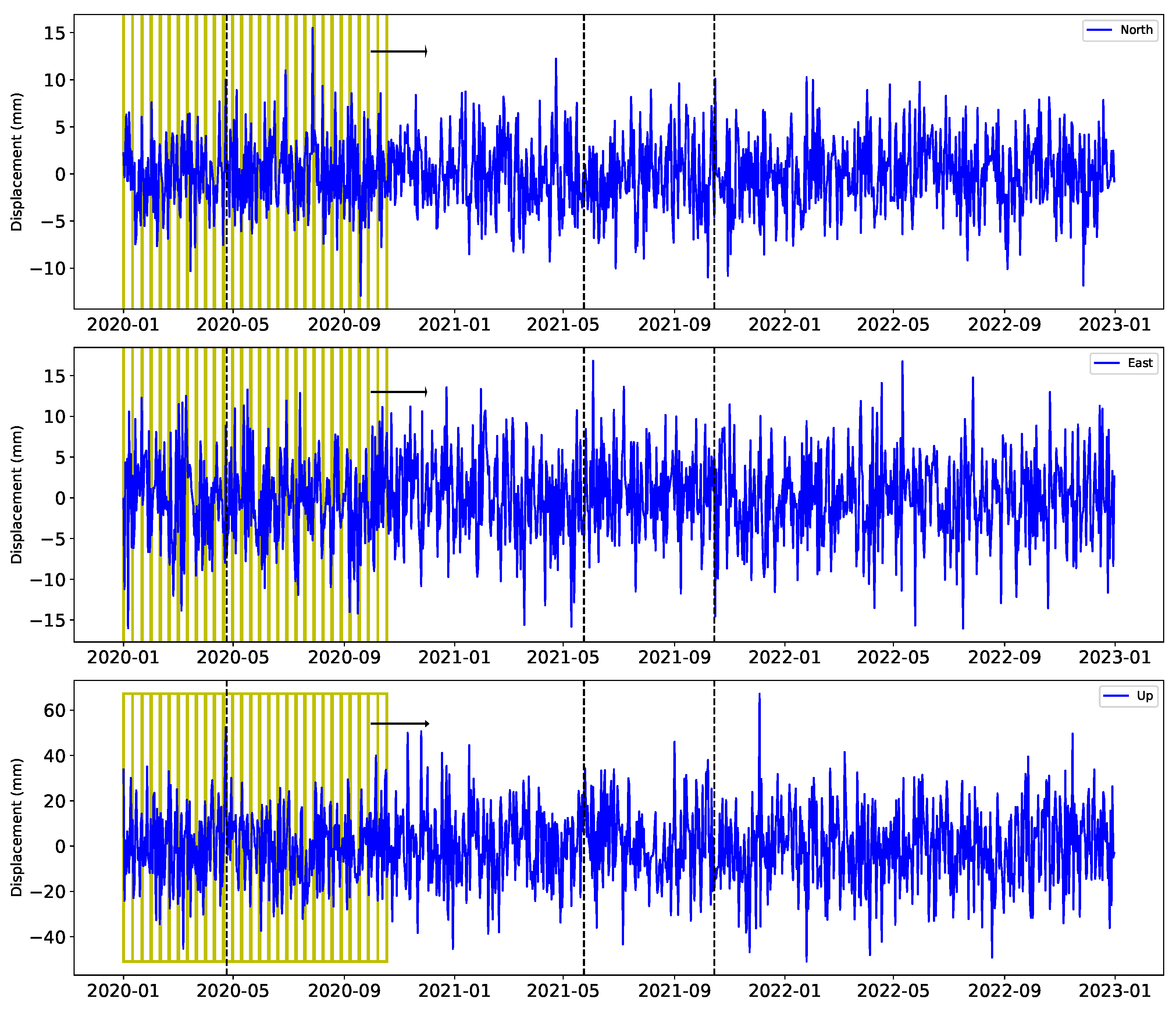
The residual analysis section aims to rigorously evaluate the performance of the XGBoost and LSTM models in detecting discontinuities within the GNSS time series data. After removing the linear trends and seasonal variations, we assume that the residuals primarily represent tectonic signals, including potential discontinuities caused by seismic events. In this study, we define a discontinuity as a sudden change in the GNSS time series exceeding a threshold value of 10 mm. We also investigate the impact of varying the threshold to 5 mm and 20 mm to investigate the robustness of the initial model. By comparing the model-detected discontinuities with an established earthquake catalog, we aim to validate the accuracy and reliability of our models. This analysis not only highlights the strengths and weaknesses of the XGBoost and LSTM models but also provides insights into the effectiveness of different threshold values in capturing significant seismic events. Figure 7 shows the detrended residual time series for the ONIY station and the segmentation of the time series for the discontinuity analysis. Here, it is worthy noting that we mostly follow the aforementioned strategies and parameters for the residual analysis as well. The most important difference is implementing a displacement threshold for the feature classification.
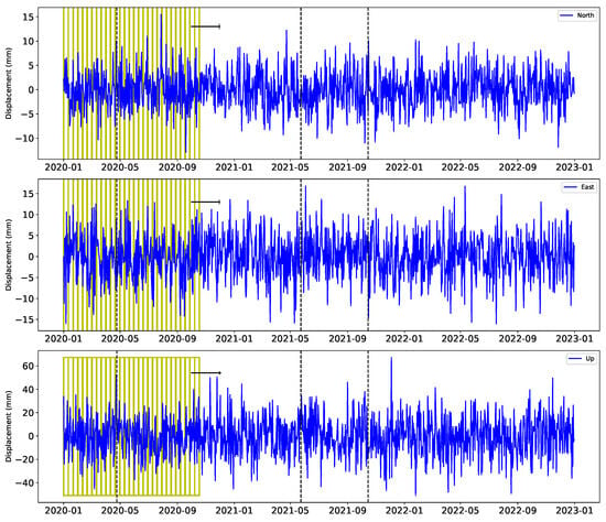
Figure 7.
Detrended residual signal. The focus on the detrended residual signal facilitates the detection of short-term patterns and anomalies visually. The yellow rectangles illustrate the segmentation of the residual signal into 21-day windows. Each window advances by 10 days, allowing for a thorough analysis of the data in overlapping segments. The segmented windows move sequentially through the entire dataset.
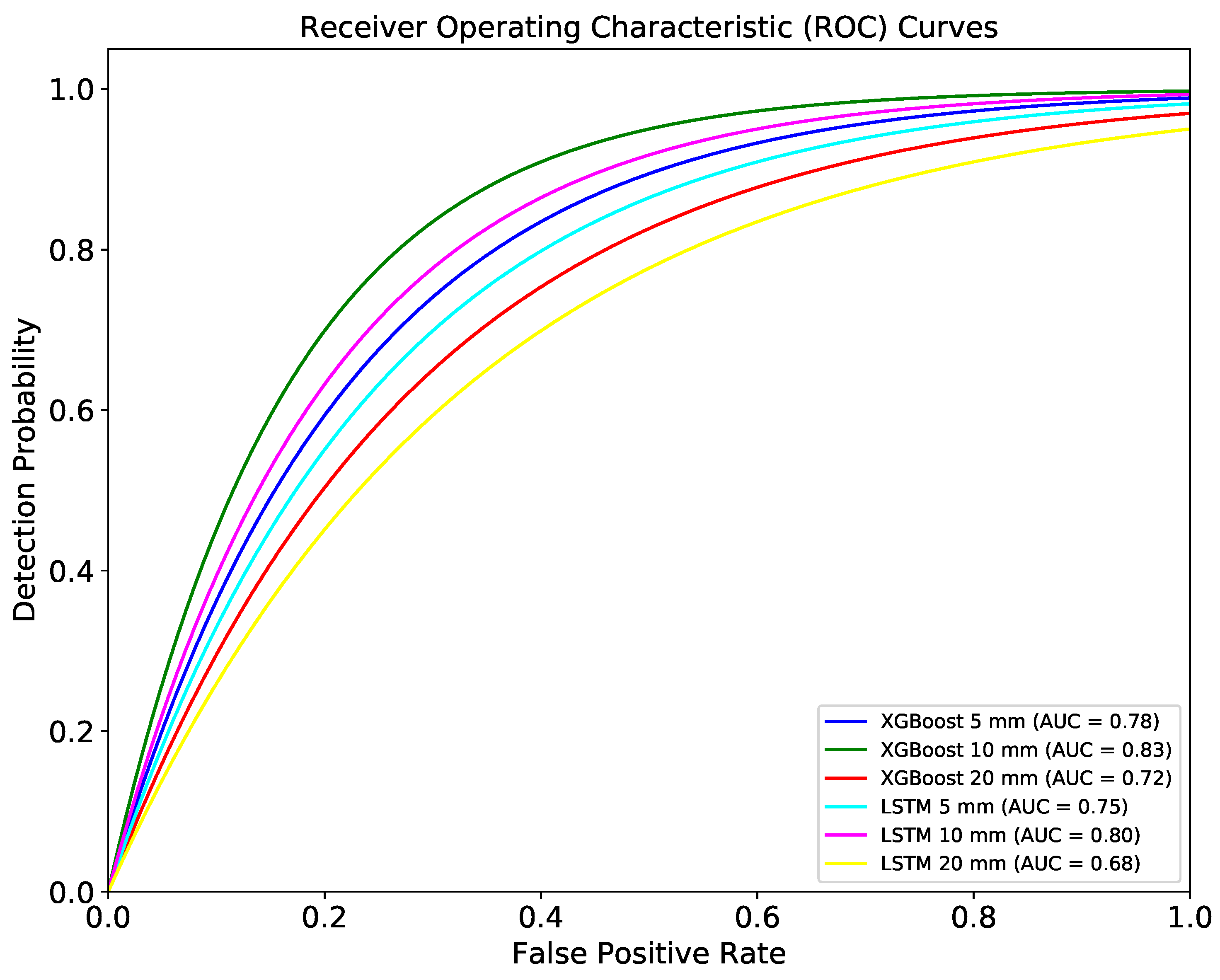
ROC and AUC are particularly valuable over the residual analysis because they allow us to assess how well the models can identify true discontinuities within the residuals of the GNSS time series. By comparing the ROC curves of both models, we can obtain further information into their relative performance and robustness under varying threshold conditions. Additionally, AUC provides a single scalar value that summarizes the models’ performance, making it easier to compare and interpret results. We calculate the ROC curves and AUC values for both models across different threshold values (5 mm, 10 mm, and 20 mm) to understand the impact of threshold selection on model performance. The ROC and AUC curves provide a detailed evaluation of the XGBoost and LSTM models’ performance in detecting discontinuities within the residuals of the GNSS time series. As shown in Figure 8, the ROC curves for both models were plotted for three different threshold values as 5 mm, 10 mm, and 20 mm. The AUC values for each threshold provide a clear quantitative measure of the models’ ability to discriminate between true discontinuities and false detections. For the XGBoost model, the AUC values were 0.79, 0.83, and 0.76 for the 5 mm, 10 mm, and 20 mm thresholds, respectively. This indicates that the model performs exceptionally well in distinguishing discontinuities, with the highest discriminative power observed at the 10 mm threshold. The LSTM model, on the other hand, achieved AUC values of 0.74, 0.78, and 0.76 for the same thresholds.
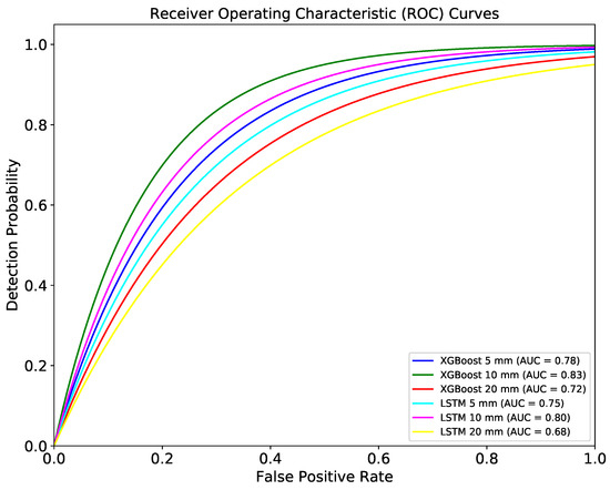
Figure 8.
The ROC (Receiver Operating Characteristic) curves along with their corresponding AUC (Area Under the Curve) values for various models. The ROC curves depict the detection probabilities for models at three different threshold values: 5 mm, 10 mm, and 20 mm. Each curve represents the performance of a model in distinguishing between classes at these specific thresholds. It is noteworthy that the model evaluated at the 10 mm threshold exhibits the best fit, as evidenced by its better ROC curve and the highest AUC value among the compared thresholds.
The ROC curves highlight that both models maintain high true positive rates with relatively low false positive rates, particularly at the 10 mm threshold. However, the XGBoost model consistently outperforms the LSTM model, as evidenced by its higher AUC values. This suggests that XGBoost has a better capability of accurately detecting discontinuities within the residual data, making it a more reliable choice for this application.
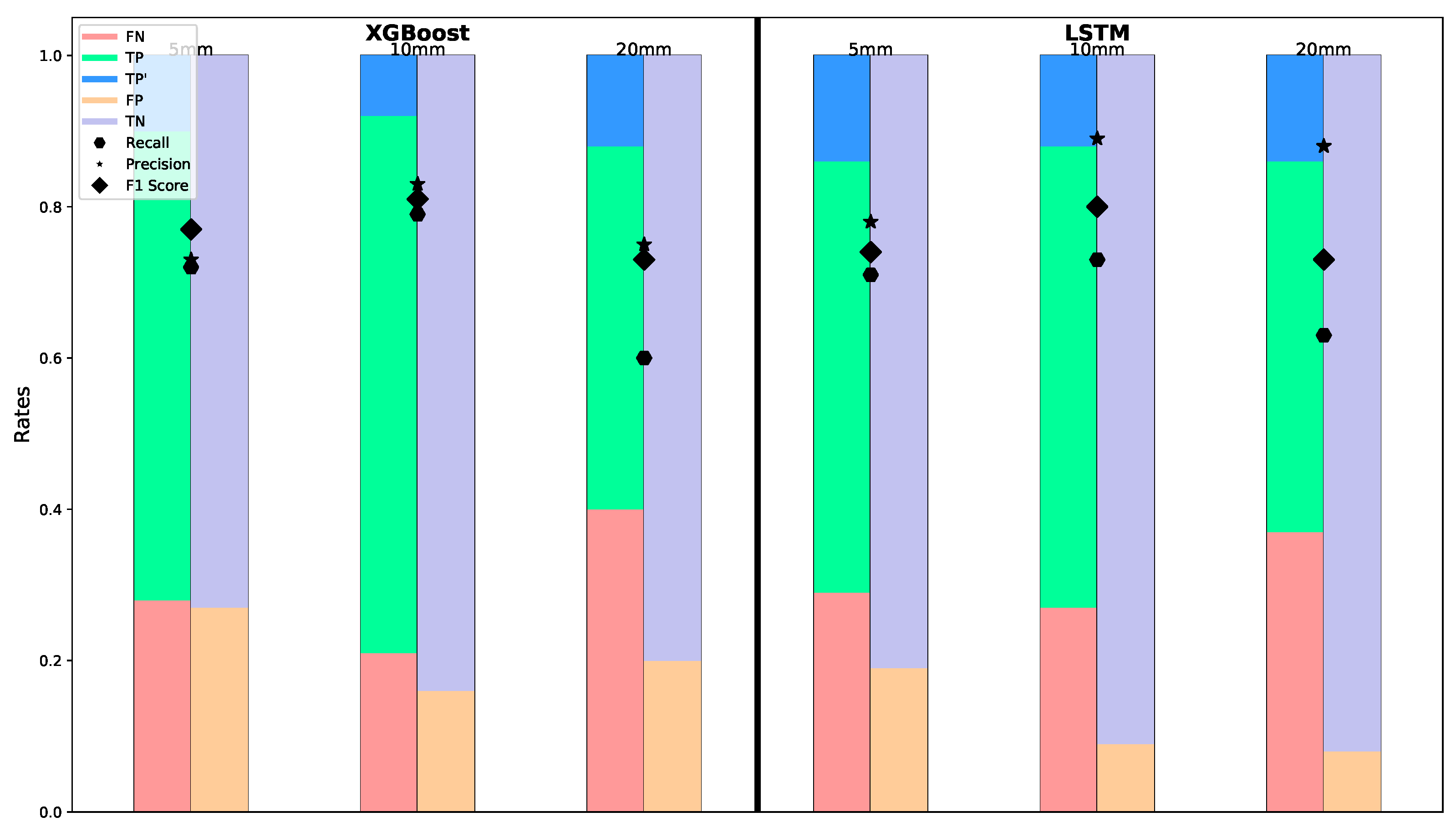
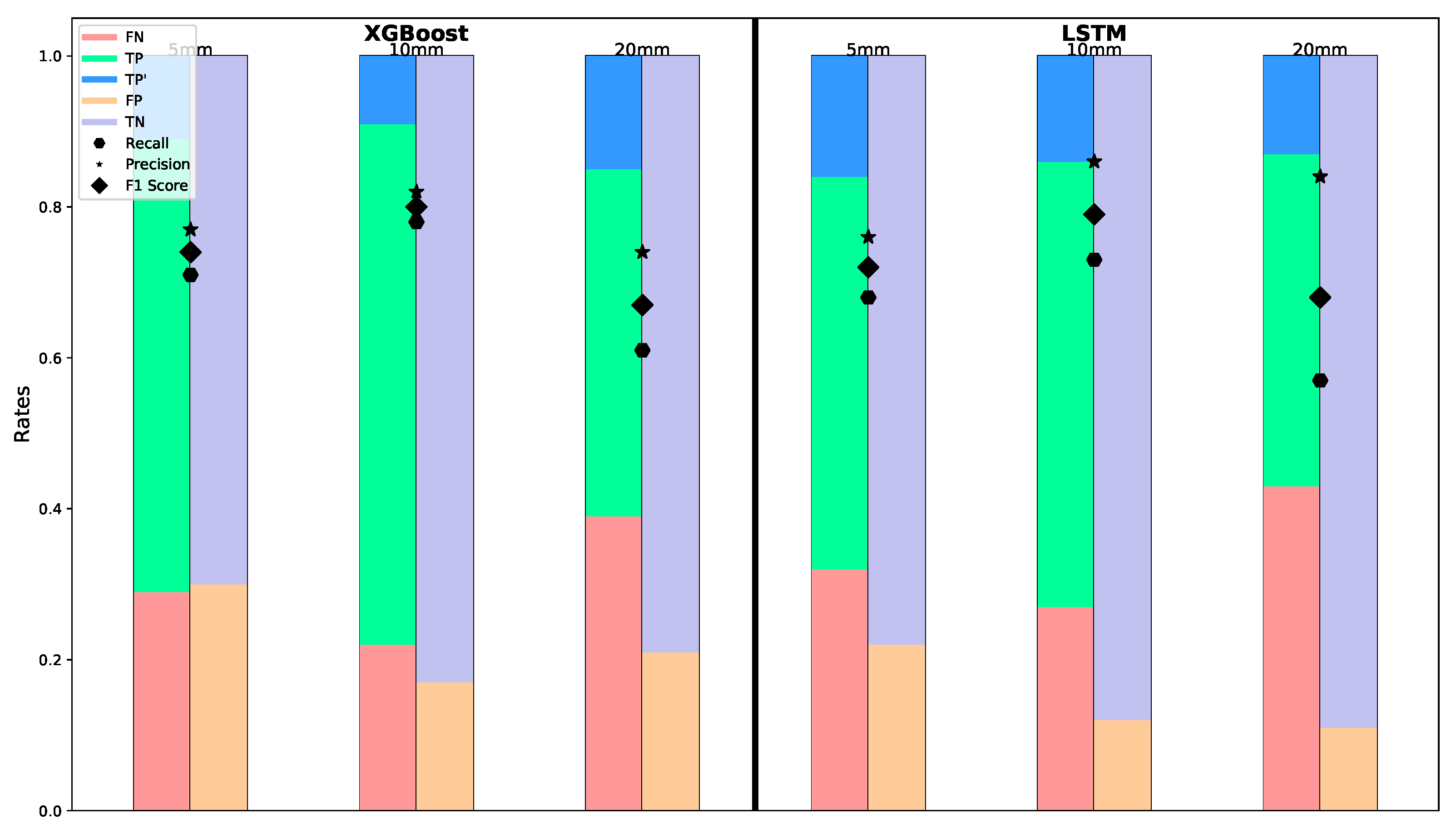
The confusion matrix results for the training phase of the XGBoost and LSTM models reveal extra implications for their performance in detecting discontinuities within the GNSS time series data. For the XGBoost model, the confusion matrix indicates a 0.79 true positive rate (TP+TP′), a 0.16 false positive rate, and a 0.21 false negative rate. These results suggest that the model has a high true positive rate, indicating its capability of correctly identifying discontinuities. The relatively low number of false positives and false negatives further shows the model’s precision and recall, reinforcing its robustness in handling the training data. In contrast, the LSTM model’s confusion matrix shows 0.73 true positive, 0.09 false positive, and 0.27 false negative rates, as shown in Figure 9. While the LSTM model also demonstrates a high true positive rate, it also exhibits a lower number of false positives compared to the XGBoost model. It might be interpreted that a lower false positive rate indicates the reliability of the LSTM model in terms of minimizing incorrect identifications of non-events as events.
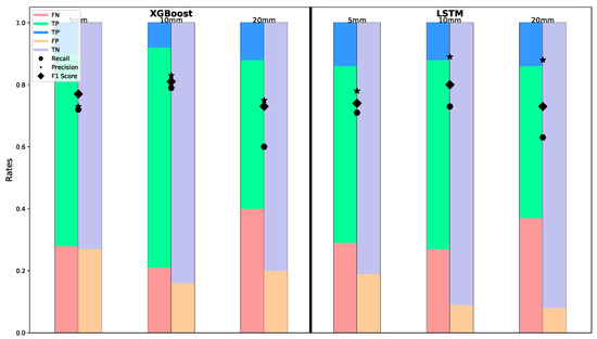
Figure 9.
Histograms illustrating the distribution of the elements of the confusion matrix for each model. Hexagons represent the recall, indicating the proportion of actual positives correctly identified. Stars show the precision, which can be interpreted as the proportion of predicted positive rates that are correctly identified. The F1 scores identified with a diamond provide a harmonic mean of precision and recall for each model.
Moreover, the XGBoost model achieves an MAE of 1.94 mm, RMSE of 2.38 mm, and R² of 0.77, indicating its higher predictive accuracy and degree of explained variance. The LSTM model, with an MAE of 2.16 mm, RMSE of 2.70 mm, and R² of 0.75, performs well but lags slightly behind the XGBoost model. The precision, recall, and F1 score results provide insightful comparisons between the models. XGBoost demonstrates a balanced performance with a solid trade-off between precision and recall, indicating its robustness in correctly identifying true events while maintaining a reasonable rate of false positives. In contrast, the LSTM model shows higher precision, suggesting it is better at minimizing false positives, thus ensuring that most of its positive predictions are accurate. However, LSTM’s lower recall values to a slight weakness in realizing all true events, which might lead to missing some actual events. Despite this, the F1 scores of both models are comparable, indicating that each offers valuable strengths depending on the specific requirements of minimizing false positives or maximizing the detection of true events.
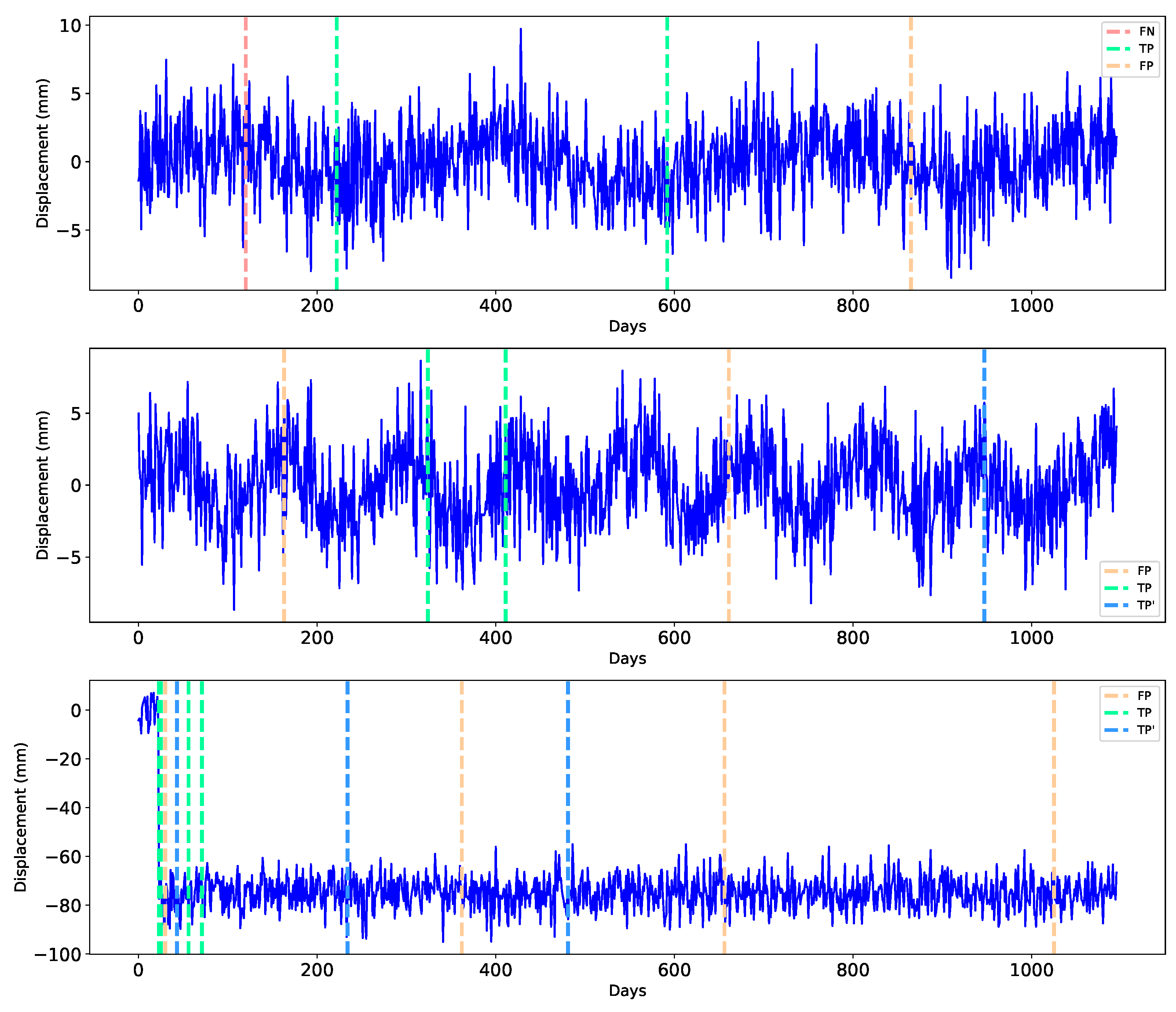
Figure 10 illustrates the time series of BTMN station and actual and detected (both true and false) discontinuities. During the training phase of our analysis, both models were evaluated for their ability to accurately detect discontinuities in GNSS time series data from stations located within 100 km of actual seismic events. For this part of the study, we focused on 80 events to train the models. The True Positive (TP) rates were particularly notable for the XGBoost model, indicating its capability of accurately identifying discontinuities. For instance, at station BTMN, XGBoost identified 8 out of the 10 events correctly, while the LSTM model identified 6. This higher TP rate for XGBoost indicates its effectiveness in learning and predicting precise discontinuities during the training phase.

Figure 10.
Prediction performance of the best fitting model across three different sites. Dashed lines on the figure represent specific epochs corresponding to true positives (TP), false positives (FP), false negatives (FN), and an additional true positive (TP′) for each site. These markers help in understanding the model’s prediction accuracy at different points in time. The bottom subplot is the ELAZ station, which is the nearest station to the epicenter of the Elazig earthquake and aftershocks that occurred.
Conversely, the LSTM model exhibited a slight advantage in reducing FPs, highlighting its sensitivity in detecting subtle changes. At station CANK, LSTM showed one FP compared to three for XGBoost, demonstrating LSTM’s precision in distinguishing between true and false events. However, XGBoost maintained a lower FN rate overall, implying fewer incorrect predictions of discontinuities. XGBoost recorded two FN cases, whereas LSTM had three, suggesting that LSTM’s architecture is slightly more adept at capturing less obvious shifts.
When evaluating the True Positive Prime (TP′) values, which reflect detection within the same window but not on the exact date, both models performed sufficiently well. For example, XGBoost achieved nine TP′ cases, while LSTM recorded seven for the ELAZ station. This shows that both models can reliably identify shifts within a reasonable timeframe, though XGBoost exhibited slightly better accuracy.
The confusion matrix results for the testing phase, on the other hand, have a very similar pattern with training data. It indicates both models are capable of learning sufficient information from their training process The similar rate with validation also implies the selection of hyperparameters. The precision of the XGBoost model in the testing phase stands at 0.82, recall at 0.78, and F1 score at 0.80, while the LSTM model has 0.86, 0.73 and 0.79, respectively (Figure 11). The LSTM model scores reflect a balanced but slightly lower performance across these metrics compared to the XGBoost model.

Figure 11.
The confusion matrix elements obtained during the prediction step. We follow the same legend as presented in Figure 9 for consistency and ease of reference. It seems that the model’s predictive performance, by examining the distribution and frequency of each confusion matrix element and score, is sufficiently close to the test results, albeit a small decrease.
The comparison of the evaluation metrics, with XGBoost achieving an overall precision of 82% and recall of 78%, and confusion matrix results indicates the model’s robustness and reliability in detecting discontinuities within the GNSS time series data. In our analysis, we evaluated the performance of XGBoost and LSTM models in detecting discontinuities within GNSS time series data across stations located within 100 km of actual seismic events. Based on the analysis of over 460 events that occurred within the relevant time frame and consistent with the GNSS time series in the zone of interest, both models demonstrated significant capabilities, each with distinct strengths. The True Positive (TP) rates were higher for the XGBoost model, indicating its ability to detect exact discontinuities accurately. For instance, the XGBoost model has a 0.9 TP for the MARD station which is one of the best scores among the stations.
However, the LSTM model showed better performance in terms of the False Positive (FP) rate, showing that it made fewer incorrect predictions of discontinuities when none existed. This suggests that LSTM is more precise in its predictions, reducing the likelihood of false alarms. For the station BEYS, LSTM had two FP cases compared to five for XGBoost, indicating that LSTM is more sensitive to discriminating oscillations with discontinuities. This sensitivity can be critical in ensuring that minor but significant shifts are not overlooked. The LSTM model’s ability to interpret minor discontinuities, reflected in its 86% precision rate, can be attributed to its recurrent neural network architecture, which effectively captures temporal dependencies and patterns over time. Additionally, the True Negative (TN) rates were fairly comparable between the two models, suggesting that both models are equally effective in correctly identifying periods of stability in the time series data. Furthermore, when considering True Positive Prime (TP′) values, both models showed considerable effectiveness. For instance, five TP′ cases were detected for both models at the RHIY station. This indicates that both models can identify shifts within reasonable proximity to the actual event date.
Our analysis reveals that the best-fitting models for both methods demonstrate a robust ability to detect seismic events (Mw ≥ 4.0). Particularly, these models achieve an impressive precision of approximately 85%. This high precision indicates the reliability of our models in identifying significant seismic events, thereby reducing the rate of false positives and enhancing the overall accuracy of our predictions. Notably, it is important to reiterate that we obtained this score by only taking into account the nearest station of an earthquake. On the other hand, both models successfully detected all discontinuities corresponding to seismic events larger than Mw 6.0 for all stations within the 100 km radius buffer zone. The consistent detection of these larger events highlights the models’ reliability particularly concerning larger events that can be evaluated as "hazards".
5. Discussion
The application of machine learning models in GNSS time series analysis represents a significant advancement in geophysical research, particularly in the detection of discontinuities associated with seismic events. Our study employed XGBoost and LSTM models to analyze GNSS time series data from continuous stations, spanning over a decade. The comparison of our results with existing literature shows both the capability of our approach and areas enhancing model performance with further refinement.
Our choice of XGBoost and LSTM models shows their effectiveness in handling complex and noisy datasets. XGBoost, known for its robustness in handling non-linear relationships and its ability to manage noise, performed exceptionally well in detecting discontinuities within the GNSS time series. This finding is consistent with the work of Gao et al. [20], and Li et al. [23] also concluded XGBoost is effective in GNSS time series forecasting, particularly in scenarios where data complexity is a significant challenge. The performance of LSTM, while slightly lower than that of XGBoost, still demonstrated considerable effectiveness in detecting long-term dependencies within the GNSS data. This is consistent with findings from Wang et al. [19], who highlighted LSTM’s strengths in time series prediction tasks. However, our study also confirmed some of the limitations observed by Wang et al. [19], particularly in detecting abrupt changes or discontinuities. This suggests that while LSTM is powerful for detecting trends, it may require enhancement or hybridization with other models, such as the VMD-LSTM hybrid approach used by Chen et al. [22] to improve its performance in detecting sharp transitions.
Crocetti et al. [18] emphasized the importance of machine learning in detecting coseismic displacements, which directly relates to our study’s focus on discontinuity detection. The consistent detection of larger seismic events (Mw ≥ 6.0) by both XGBoost and LSTM models in our analysis supports the conclusions presented by Crocetti et al. [18] about the potential of machine learning in geophysical monitoring. Our study further confirms that tree-based models like XGBoost are particularly adept at this task, as evidenced by their higher precision and recall rates.
The effectiveness of machine learning in GNSS time series analysis is further supported by Gao et al. [20], who compared traditional least squares and machine learning approaches in surface deformation monitoring. Their findings, which showed the effectiveness of machine learning models in handling complex datasets, parallel our results and emphasize the value of applying such models to GNSS data. However, Gao et al. [20]. also indicated the importance of model validation across different geophysical contexts, also pointed out by our study, aiming to address model performances across various stations and seismic events.
While our study focused on discontinuity detection, the broader application of machine learning in GNSS time series analysis is explored by Xie et al. [24]. They employed a CNN-GRU hybrid model, highlighting the potential benefits of incorporating convolutional layers to extract spatial features from GNSS data before applying recurrent layers for temporal analysis. While our study did not explore this hybrid approach, the success of Xie et al. [24] suggests that integrating CNNs could enhance the feature extraction process in such models.
6. Conclusions
This study has demonstrated the effectiveness of machine learning algorithms, specifically XGBoost and Long Short-Term Memory (LSTM) networks, in detecting discontinuities in GNSS time series data from the tectonically active Anatolian region. By leveraging over 13 years of continuous GNSS observations from 15 stations, we were able to refine and validate models that significantly improve the detection of seismic and geophysical events.
The preprocessing step, which included the removal of linear trends and seasonal signals, might be critical in preparing the data for accurate model training and analysis for discontinuity detection. These steps ensured that the residuals mainly contained the tectonic signals and other short-term variations of interest, providing a cleaner dataset for the machine learning models to analyze. Both models have sufficient scores to analyze the trend and periodic signals for each time series. It can be concluded that machine learning algorithms are also effective in detecting periodic signals, such as those based on atmospheric conditions [21,22].
Our analysis revealed that XGBoost consistently outperformed LSTM in terms of True Positive (TP) rates, indicating its ability to accurately detect precise discontinuities. LSTM’s lower False Positive (FP) rate further emphasized its precision, making it a more reliable choice for identifying true discontinuities without generating false alarms. This characteristic of LSTM highlights its potential usefulness in applications where detecting minor yet significant changes is critical.
The robust performance in detecting discontinuities (corresponding to Mw ≥ 4.0) for both models, albeit for the nearest stations, indicates the potential of these new methods together with the further high spatial resolution for both seismic and geodetic networks. This capability indicates the models’ reliability in identifying significant seismic impacts, which is crucial for understanding seismic hazards.
The inclusion of True Positive Prime (TP′) values in our analysis provided additional insights into the models’ ability to detect shifts within a reasonable timeframe, even if not on the exact event date. This aspect is particularly important for practical applications where exact timing might not always be possible, but the detection of shifts within a certain window is still valuable.
Future work can focus on further enhancing model accuracy, particularly in detecting smaller transient and slow slip events, which require more sophisticated approaches. Improving the sensitivity and precision of these models can lead to better real-time monitoring and prediction capabilities, ultimately contributing to more effective seismic hazard assessments and risk mitigation strategies.
Overall, this study has successfully demonstrated the potential of machine learning algorithms in enhancing the analysis of GNSS time series data. The results highlight the advantages of integrating ML algorithms into geophysical research, providing deeper insights into tectonic processes and improving the accuracy of seismic hazard assessments. However, as mentioned by Crocetti et al. [18], these two methods, along with other algorithms, should be employed in future studies across different tectonically active regions to further test their reliability and contribute to the broader field of geodesy and geophysics.
Supplementary Materials
The following supporting information can be downloaded at: https://www.mdpi.com/article/10.3390/rs16173309/s1.
Author Contributions
Conceptualization, V.Ö. and S.E.; methodology, V.Ö. and S.E.; software, V.Ö.; validation, V.Ö.; formal analysis, V.Ö.; investigation, V.Ö., S.E. and E.T.; resources, V.Ö., S.E and E.T.; data curation, V.Ö.; writing—original draft preparation, V.Ö.; writing—review and editing, S.E. and E.T.; visualization, V.Ö.; supervision, S.E. and E.T. All authors have read and agreed to the published version of the manuscript.
Funding
This research received no external funding.
Data Availability Statement
The raw GNSS time series data utilized in this study are available in the electronic Supplementary Materials that provides comprehensive access to the dataset, enabling further exploration and validation of the results presented in this study.
Acknowledgments
We extend our gratitude to the editor and anonymous reviewers for their valuable comments and suggestions, which have significantly enhanced the quality of our study. We would like to express our thanks to Seda Ozarpaci, Alpay Ozdemir and Efe Ayruk for their support during the data processing of GNSS time series and model analysis. Their expertise and assistance were crucial in advancing this research. We also extend our special thanks to the General Directorate of the Mapping Unit of Turkey and Ali Ihsan Kurt for supplying the necessary data. Our research greatly benefited from the use of Generic Mapping Tools (GMT) and several Python libraries, including NumPy, pandas, scikit-learn, and TensorFlow [42,43,44,45,46]. These tools and libraries were instrumental in visualizing and analyzing the solutions presented in this study. The numerical calculations reported in this paper were partially performed at TUBITAK ULAKBIM, High Performance and Grid Computing Center (TRUBA resources).
Conflicts of Interest
The authors declare no conflicts of interest.
Abbreviations
The following abbreviations are used in this manuscript:
| GNSS | Global Navigational Satellite System |
| TUSAGA | Turkish National Continuous GNSS Network |
| RCMT | Regional Centroid Moment Tensor |
| Mw | Moment Magnitude |
| CME | Common Mode Error |
| ML | Machine Learning |
| LSTM | Long Short-Term Memory |
| NAF | North Anatolian Fault |
| EAF | East Anatolian Fault |
| IGS | International GNSS Service |
| AMLSTM NN | Attention Mechanism with Long Short-Time Memory Neural Network |
| TP | True Positive |
| TN | True Negative |
| FP | False Positive |
| FN | False Negative |
| TP′ | True Positive Prime |
| RNN | Recurrent Neural Network |
| MSE | Mean Squared Error |
| MAE | Mean Absolute Error |
| RMSE | Root Mean Squared Error |
| R2 | R-squared (Coefficient of Determination) |
| ROC | Receiver Operating Characteristic |
| AUC | Area Under the Curve |
| GMT | Generic Mapping Tools |
Appendix A
In this section, we describe the machine learning methods adopted for the analysis of GNSS time series data. We particularly focus on two techniques: eXtreme Gradient Boosting (XGBoost) and Long Short-Term Memory (LSTM) networks. These methods were selected due to their demonstrated effectiveness in handling complex, high-dimensional time series data.
XGBoost is an implementation of gradient-boosted decision trees designed for speed and performance. It is widely used in many machine learning applications due to its robustness and efficiency. XGBoost builds an ensemble of decision trees sequentially, where each subsequent tree attempts to correct the errors of the previous ones. The objective function in XGBoost combines a loss function and a regularization term. The loss function measures how well the model fits the training data, while the regularization term penalizes model complexity to prevent overfitting. The objective function is formulated as:
where l is a differentiable convex loss function that measures the difference between the prediction and the target . The term constrains the complexity of the model (e.g., the number of leaves in the trees and the norm of the weights). The model is trained in an additive manner, where each iteration adds a new tree that minimizes the objective function. The prediction for a data point i at the t-th iteration is given by:
The architecture of an XGBoost model involves the sequential addition of decision trees. Each tree aims to reduce the residual errors of the previous trees. This process continues until the model reaches a specified number of trees or the error no longer decreases significantly. Hyperparameters are also critical to the performance of XGBoost. We employed a grid search with cross-validation to find the optimal set of hyperparameters. Table A1 includes the key hyperparameters for this method.

Table A1.
Key hyperparameters for the adopted XGBoost algorithm.
Table A1.
Key hyperparameters for the adopted XGBoost algorithm.
| Hyperparameter | Explanation |
|---|---|
| Number of trees | Number of boosting rounds |
| Learning Rate | Step size shrinkage used to prevent overfitting |
| Maximum depth | Maximum depth of a tree |
| Minimum Child Weight | Minimum sum of instance weight (hessian) needed in a child |
| Subsample | Fraction of observations to be randomly sampled for each tree |
| Column sample | Fraction of features to be randomly sampled for each tree |
XGBoost provides a way to calculate the importance of each feature by how much it contributes to improving the model’s performance. This is useful for understanding which features are most influential in predicting the target variable. Our model for analyzing GNSS time series comprises preprocessed GNSS raw time series as the input layer. It then sequentially creates a decision-tree-type structure to improve the model. The final step is the aggregation of the predictions from all the trees to produce the final output.
Long Short-Term Memory (LSTM) networks, on the other hand, are a type of recurrent neural network (RNN) capable of learning long-term dependencies, which makes them particularly effective for time series prediction tasks. LSTM networks are designed to overcome the limitations of traditional RNNs, which require long-term dependencies due to issues such as vanishing and exploding gradients. LSTMs address this by incorporating memory cells that can maintain their state over extended periods. Each LSTM unit consists of three main gates: the input gate, the forget gate, and the output gate. These gates control the flow of information into, out of, and within the memory cell, allowing the network to retain or discard information as needed. The mathematical formulation of an LSTM unit can be summarized as:
where is the sigmoid function, is the hyperbolic tangent function, and ⊙ denotes element-wise multiplication. is the hidden state vector at time step t. This vector contains the output from the LSTM cell, which is used as input for the next time step and can be passed to subsequent layers in a deep network. presents the input vector, for our analysis, and represents the features extracted from the GNSS data for the current time step. are the bias vectors for the input gate, forget gate, output gate, and cell state update, respectively. These biases are added to the linear combinations of the inputs and previous hidden states to shift the activation functions. are the weight matrices transforming the concatenation of the input vector and the previous hidden state linearly.
The architecture of an LSTM model typically consists of multiple layers of LSTM units, followed by dense layers to produce the final output. In terms of GNSS time series analysis, the LSTM network is designed to detect the temporal dependencies in the data, such as trends, seasonal patterns, and abrupt changes due to tectonic events. Training an LSTM model involves feeding the GNSS time series data into the network, adjusting the weights and biases through backpropagation, and minimizing the loss function. The loss function typically used for regression tasks is the mean squared error (MSE). We employed the Adam optimizer, one of the commonly used ones, to update the model parameters due to its efficiency and ability to handle sparse gradients. Grid search or random search methods can be adopted to systematically explore different combinations of hyperparameters and identify the optimal configuration. Key parameters of the LSTM algorithm are shown in Table A2.

Table A2.
Key hyperparameters for the selected LSTM method.
Table A2.
Key hyperparameters for the selected LSTM method.
| Hyperparameter | Explanation |
|---|---|
| Number of Layers | The depth of the network |
| Number of Units per Layer | The number of memory cells in each layer |
| Dropout Rate | The fraction of input units to drop during training to prevent overfitting |
| Learning Rate | The step size for the optimizer |
| Batch Size | The number of samples per gradient update |
| Number of Epochs | The number of times the entire dataset is passed through the network during training |
References
- Blewitt, G.; Hammond, W.C.; Kreemer, C.; Plag, H.P.; Stein, S.; Okal, E. GPS for real-time earthquake source determination and tsunami warning systems. J. Geod. 2009, 83, 335–343. [Google Scholar] [CrossRef]
- Mao, A.; Harrison, C.G.A.; Dixon, T.H. Noise in GPS coordinate time series. J. Geophys. Res. Solid Earth 1999, 104, 2797–2816. [Google Scholar] [CrossRef]
- Dong, D.; Fang, P.; Bock, Y.; Cheng, M.K.; Miyazaki, S. Anatomy of apparent seasonal variations from GPS-derived site position time series. J. Geophys. Res. Solid Earth 2002, 107, ETG 9-1–ETG 9-16. [Google Scholar] [CrossRef]
- Williams, S. The effect of coloured noise on the uncertainties of rates estimated from geodetic time series. J. Geodesy 2003, 76, 483–494. [Google Scholar] [CrossRef]
- King, M.A.; Williams, S.D.P. Apparent stability of GPS monumentation from short-baseline time series. J. Geophys. Res. Solid Earth 2009, 114, B10403. [Google Scholar] [CrossRef]
- Jiang, Y.; Wdowinski, S.; Dixon, T.H.; Hackl, M.; Protti, M.; Gonzalez, V. Slow slip events in Costa Rica detected by continuous GPS observations, 2002–2011. Geochem. Geophys. Geosyst. 2012, 13, Q04006. [Google Scholar] [CrossRef]
- Gazeaux, J.; Williams, S.; King, M.; Bos, M.; Dach, R.; Deo, M.; Moore, A.W.; Ostini, L.; Petrie, E.; Roggero, M.; et al. Detecting offsets in GPS time series: First results from the detection of offsets in GPS experiment. J. Geophys. Res. Solid Earth 2013, 118, 2397–2407. [Google Scholar] [CrossRef]
- Frank, W.B.; Rousset, B.; Lasserre, C.; Campillo, M. Revealing the cluster of slow transients behind a large slow slip event. Sci. Adv. 2018, 4, eaat0661. [Google Scholar] [CrossRef]
- Bos, M.; Fernandes, R.; Williams, S.; Bastos, L. Fast error analysis of continuous GPS observations. J. Geodesy 2008, 82, 157–166. [Google Scholar] [CrossRef]
- Dong, D.; Fang, P.; Bock, Y.; Webb, F.; Prawirodirdjo, L.; Kedar, S.; Jamason, P. Spatiotemporal filtering using principal component analysis and Karhunen-Loeve expansion approaches for regional GPS network analysis. J. Geophys. Res. Solid Earth 2006, 111, B03405. [Google Scholar] [CrossRef]
- Williams, S.D.P.; Bock, Y.; Fang, P.; Jamason, P.; Nikolaidis, R.M.; Prawirodirdjo, L.; Miller, M.; Johnson, D.J. Error analysis of continuous GPS position time series. J. Geophys. Res. Solid Earth 2004, 109, B03412-1. [Google Scholar] [CrossRef]
- Williams, S.D. CATS: GPS coordinate time series analysis software. GPS Solut. 2008, 12, 147–153. [Google Scholar] [CrossRef]
- Segall, P.; Desmarais, E.K.; Shelly, D.; Miklius, A.; Cervelli, P. Earthquakes triggered by silent slip events on Kīlauea volcano, Hawaii. Nature 2006, 442, 71–74. [Google Scholar] [CrossRef] [PubMed]
- Brown, J.R.; Beroza, G.C.; Ide, S.; Ohta, K.; Shelly, D.R.; Schwartz, S.Y.; Rabbel, W.; Thorwart, M.; Kao, H. Deep low-frequency earthquakes in tremor localize to the plate interface in multiple subduction zones. Geophys. Res. Lett. 2009, 36. [Google Scholar] [CrossRef]
- Bishop, C.M.; Nasrabadi, N.M. Pattern Recognition and Machine Learning; Springer: New York, NY, USA, 2006; Volume 4. [Google Scholar]
- Goodfellow, I.; Bengio, Y.; Courville, A. Deep Learning; MIT Press: Cambridge, MA, USA, 2016. [Google Scholar]
- Wang, J.; Nie, G.; Gao, S.; Wu, S.; Li, H.; Ren, X. Landslide Deformation Prediction Based on a GNSS Time Series Analysis and Recurrent Neural Network Model. Remote Sens. 2021, 13, 1055. [Google Scholar] [CrossRef]
- Crocetti, L.; Schartner, M.; Soja, B. Discontinuity Detection in GNSS Station Coordinate Time Series Using Machine Learning. Remote Sens. 2021, 13, 3906. [Google Scholar] [CrossRef]
- Wang, J.; Jiang, W.; Li, Z.; Lu, Y. A New Multi-Scale Sliding Window LSTM Framework (MSSW-LSTM): A Case Study for GNSS Time-Series Prediction. Remote Sens. 2021, 13, 3328. [Google Scholar] [CrossRef]
- Gao, W.; Li, Z.; Chen, Q.; Jiang, W.; Feng, Y. Modelling and prediction of GNSS time series using GBDT, LSTM and SVM machine learning approaches. J. Geodesy 2022, 96, 71. [Google Scholar] [CrossRef]
- Ruttner, P.; Hohensinn, R.; D’Aronco, S.; Wegner, J.D.; Soja, B. Modeling of Residual GNSS Station Motions through Meteorological Data in a Machine Learning Approach. Remote Sens. 2022, 14, 17. [Google Scholar] [CrossRef]
- Chen, H.; Lu, T.; Huang, J.; He, X.; Yu, K.; Sun, X.; Ma, X.; Huang, Z. An Improved VMD-LSTM Model for Time-Varying GNSS Time Series Prediction with Temporally Correlated Noise. Remote Sens. 2023, 15, 3694. [Google Scholar] [CrossRef]
- Li, Z.; Lu, T.; Yu, K.; Wang, J. Interpolation of GNSS Position Time Series Using GBDT, XGBoost, and RF Machine Learning Algorithms and Models Error Analysis. Remote Sens. 2023, 15, 4374. [Google Scholar] [CrossRef]
- Xie, Y.; Wang, J.; Li, H.; Dong, A.; Kang, Y.; Zhu, J.; Wang, Y.; Yang, Y. Deep Learning CNN-GRU Method for GNSS Deformation Monitoring Prediction. Appl. Sci. 2024, 14, 4004. [Google Scholar] [CrossRef]
- McKenzie, D. Active tectonics of the Mediterranean region. Geophys. J. Int. 1972, 30, 109–185. [Google Scholar] [CrossRef]
- Şengör, A.; Tüysüz, O.; İmren, C.; Sakınç, M.; Eyidoğan, H.; Görür, N.; Le Pichon, X.; Rangin, C. The North Anatolian Fault: A New Look. Annu. Rev. Earth Planet. Sci. 2005, 33, 37–112. [Google Scholar] [CrossRef]
- Reilinger, R.E.; Ergintav, S.; Bürgmann, R.; McClusky, S.; Lenk, O.; Barka, A.; Gurkan, O.; Hearn, L.; Feigl, K.L.; Cakmak, R.; et al. Coseismic and Postseismic Fault Slip for the 17 August 1999, M = 7.5, Izmit, Turkey Earthquake. Science 2000, 289, 1519–1524. [Google Scholar] [CrossRef]
- McKenzie, D. The East Anatolian Fault: A major structure in eastern Turkey. Earth Planet. Sci. Lett. 1976, 29, 189–193. [Google Scholar] [CrossRef]
- Fielding, E.J.; Lundgren, P.R.; Taymaz, T.; Yolsal-Çevikbilen, S.; Owen, S.E. Fault-Slip Source Models for the 2011 M 7.1 Van Earthquake in Turkey from SAR Interferometry, Pixel Offset Tracking, GPS, and Seismic Waveform Analysis. Seismol. Res. Lett. 2013, 84, 579–593. [Google Scholar] [CrossRef]
- Chousianitis, K.; Konca, A.O. Rupture Process of the 2020 M7.0 Samos Earthquake and its Effect on Surrounding Active Faults. Geophys. Res. Lett. 2021, 48, e2021GL094162. [Google Scholar] [CrossRef]
- Yıldırım, C.; Aksoy, M.E.; Özcan, O.; İşiler, M.; Özbey, V.; Çiner, A.; Salvatore, P.; Sarıkaya, M.A.; Doğan, T.; İlkmen, E.; et al. Coseismic (20 July 2017 Bodrum-Kos) and paleoseismic markers of coastal deformations in the Gulf of Gökova, Aegean Sea, SW Turkey. Tectonophysics 2022, 822, 229141. [Google Scholar] [CrossRef]
- Cakir, Z.; Doğan, U.; Akoğlu, A.M.; Ergintav, S.; Özarpacı, S.; Özdemir, A.; Nozadkhalil, T.; Çakir, N.; Zabcı, C.; Erkoç, M.H.; et al. Arrest of the Mw 6.8 January 24, 2020 Elaziğ (Turkey) earthquake by shallow fault creep. Earth Planet. Sci. Lett. 2023, 608, 118085. [Google Scholar] [CrossRef]
- McClusky, S.; Balassanian, S.; Barka, A.; Demir, C.; Ergintav, S.; Georgiev, I.; Gurkan, O.; Hamburger, M.; Hurst, K.; Kahle, H.; et al. Global Positioning System constraints on plate kinematics and dynamics in the eastern Mediterranean and Caucasus. J. Geophys. Res. Solid Earth 2000, 105, 5695–5719. [Google Scholar] [CrossRef]
- Reilinger, R.; McClusky, S.; Vernant, P.; Lawrence, S.; Ergintav, S.; Cakmak, R.; Ozener, H.; Kadirov, F.; Guliev, I.; Stepanyan, R.; et al. GPS constraints on continental deformation in the Africa-Arabia-Eurasia continental collision zone and implications for the dynamics of plate interactions. J. Geophys. Res. Solid Earth 2006, 111, B05411. [Google Scholar] [CrossRef]
- Özbey, V.; Şengör, A.; Henry, P.; Özeren, M.S.; Haines, A.J.; Klein, E.; Tarı, E.; Zabcı, C.; Chousianitis, K.; Guvercin, S.E.; et al. Kinematics of the Kahramanmaraş triple junction and of Cyprus: Evidence of shear partitioning. BSGF-Earth Sci. Bull. 2024, 195, 15. [Google Scholar] [CrossRef]
- Hochreiter, S.; Schmidhuber, J. Long Short-Term Memory. Neural Comput. 1997, 9, 1735–1780. [Google Scholar] [CrossRef]
- Chen, T.; Guestrin, C. Xgboost: A scalable tree boosting system. In Proceedings of the 22nd Acm Sigkdd International Conference on Knowledge Discovery and Data Mining, San Francisco, CA, USA, 13–17 August 2016; pp. 785–794. [Google Scholar] [CrossRef]
- Pondrelli, S.; Morelli, A.; Ekström, G.; Mazza, S.; Boschi, E.; Dziewonski, A. European–Mediterranean regional centroid-moment tensors: 1997–2000. Phys. Earth Planet. Inter. 2002, 130, 71–101. [Google Scholar] [CrossRef]
- Şengör, A.M.C.; Zabci, C. The North Anatolian Fault and the North Anatolian Shear Zone BT. In Landscapes and Landforms of Turkey; Springer International Publishing: Cham, Switzerland, 2019; pp. 481–494. [Google Scholar] [CrossRef]
- Herring, T.; King, R.; Floyd, M.; McClusky, S. Introduction to GAMIT/GLOBK, Release 10.7, GAMIT/GLOBK Documentation; Massachusetts Institute of Technology: Cambridge, MA, USA, 2018. [Google Scholar]
- Blewitt, G.; Lavallée, D. Effect of annual signals on geodetic velocity. J. Geophys. Res. Solid Earth 2002, 107, ETG 9-1–ETG 9-11. [Google Scholar] [CrossRef]
- McKinney, W. Data structures for statistical computing in Python. In Proceedings of the SciPy, Austin, TX, USA, 28–30 June 2010; Volume 445, pp. 51–56. [Google Scholar]
- Pedregosa, F.; Varoquaux, G.; Gramfort, A.; Michel, V.; Thirion, B.; Grisel, O.; Blondel, M.; Prettenhofer, P.; Weiss, R.; Dubourg, V.; et al. Scikit-learn: Machine learning in Python. J. Mach. Learn. Res. 2011, 12, 2825–2830. [Google Scholar]
- Abadi, M.; Agarwal, A.; Barham, P.; Brevdo, E.; Chen, Z.; Citro, C.; Corrado, G.S.; Davis, A.; Dean, J.; Devin, M.; et al. TensorFlow: Large-Scale Machine Learning on Heterogeneous Distributed Systems. arXiv 2016, arXiv:1603.04467. [Google Scholar] [CrossRef]
- Wessel, P.; Luis, J.F.; Uieda, L.; Scharroo, R.; Wobbe, F.; Smith, W.H.F.; Tian, D. The Generic Mapping Tools Version 6. Geochem. Geophys. Geosyst. 2019, 20, 5556–5564. [Google Scholar] [CrossRef]
- Harris, C.R.; Millman, K.J.; Van Der Walt, S.J.; Gommers, R.; Virtanen, P.; Cournapeau, D.; Wieser, E.; Taylor, J.; Berg, S.; Smith, N.J.; et al. Array programming with NumPy. Nature 2020, 585, 357–362. [Google Scholar] [CrossRef]
Disclaimer/Publisher’s Note: The statements, opinions and data contained in all publications are solely those of the individual author(s) and contributor(s) and not of MDPI and/or the editor(s). MDPI and/or the editor(s) disclaim responsibility for any injury to people or property resulting from any ideas, methods, instructions or products referred to in the content. |
© 2024 by the authors. Licensee MDPI, Basel, Switzerland. This article is an open access article distributed under the terms and conditions of the Creative Commons Attribution (CC BY) license (https://creativecommons.org/licenses/by/4.0/).

