A Potential Link between Space Weather and Atmospheric Parameters Variations: A Case Study of November 2021 Geomagnetic Storm

Abstract

On 4 November 2021, during the rising phase of solar cycle 25, an intense geomagnetic storm (Kp = 8−) occurred. The effects of this storm on the outer magnetospheric region up to the ionospheric heights have already been examined in previous investigations. This work is focused on the analysis of the solar wind conditions before and during the geomagnetic storm, the high-latitude electrodynamics conditions, estimated through empirical models, and the response of the atmosphere in both hemispheres, based on parameters from the ECMWF ERA5 atmospheric reanalysis dataset. Our investigations are also supported by counter-test analysis and Monte Carlo tests. We find, for both hemispheres, a significant correspondence, within 1–2 days, between high-latitude electrodynamics variations and changes in the temperature, specific humidity, and meridional and zonal winds, in both the troposphere and stratosphere. The results indicate that, in the complex solar wind–atmosphere relationship, a significant role might be played by the intensification of the polar cap potential. We also study the reciprocal relation between the ionospheric Joule heating, calculated from a model, and two adiabatic invariants used in the analysis of solar wind turbulence.

1. Introduction

Earth’s atmosphere and its ionized part, the ionosphere, are influenced by several processes of external origin, i.e., solar and magnetospheric processes [1]. Solar electromagnetic radiation and solar wind (SW) particle flux deeply affect the circumterrestrial environment. In particular, solar wind energy is transmitted to the different layers of the atmosphere through magnetospheric processes. For example, energetic particle precipitation at auroral latitudes from the radiation belts and magnetic Field-Aligned Currents closing in the high-latitude ionosphere are very important in producing changes in the structure of the atmosphere. The electron precipitation during magnetospheric storms and substorms plays a role, by ionization, in the atmospheric chemical composition and conductivity variations [2,3,4,5].

These variations are important in determining the troposphere structure, together with the variations in the polar cap electrodynamics associated with the variable SW electric field [6].

Recently, an evidence of SW-related periodicities has been found in the variations of different parameters of the troposphere, stratosphere, mesosphere, and thermosphere, at low-orbit satellites and over Antarctica [1,7,8,9,10,11,12]. In particular, Regi et al. [11] observed a statistically significant correspondence between fluctuations in atmospheric parameters (temperature and zonal wind in the troposphere and stratosphere) and fluctuations in the polar cap potential, which is connected to the SW electric field; the polar cap potential fluctuations appear strongly related to the temperature and zonal wind over Antarctica (i.e., in the polar cap, 75°S–90°S), while such a relationship decreases quickly at lower latitudes reaching minimum values at latitudes < 65°S, i.e., at latitudes lower than the average equatorward auroral oval border.

Such results support the idea that the SW electric field has a important role in the high-latitude lower atmospheric dynamics. A possible mechanism, according to Tinsley et al. [5] and Lam and Tinsley [6], is that the variations in the polar cap potential could modify the current system in the global electric circuit between the ionosphere and ground. In particular, the vertical downward current density produces a tropospheric and stratospheric response, which would be due to the charging of clouds with effects on the cloud microphysics and, in turn, on cloud cover and precipitation.

Voiculescu et al. [13] found a significant positive correlation between the interplanetary electric field (IEF) and cloud cover at low altitudes during periods characterized by the duskward y-component of IEF (which corresponds to the southward z-component of the interplanetary magnetic field, $B_z<0$), particularly evident at high latitudes and simultaneously in both the hemispheres; similarly, Regi et al. [12] found that cloud cover, temperature and specific humidity significantly change following the increase in geomagnetic activity within 2 days during periods characterized by $B_z<0$, concluding that the intensification of the polar cap potential difference plays an important role in the solar wind–atmosphere coupling. The connection between solar activity and changes in atmospheric parameters can be found over different timescales. While the connection between the activity of the sun and the climate over large timescales has been extensively studied and confirmed, less scientific literature is available on how processes related to space weather can lead to changes in Earth’s atmosphere at smaller timescales.

Research in recent decades has particularly focused on finding links between the changing activity of the sun and processes in Earth’s atmosphere lasting not less than several days or years. Only relatively recently have scientists put efforts into understanding how geomagnetic activity can affect the weather over timescales of less than a week. Most of them suggested that there is an important downward impact from the SW to the middle and then lower atmosphere that influences weather development.

Prikryl et al. [14], for example, found a connection between SW activity and extratropical cyclones in the northern hemisphere. They hypothesized that high-speed SWs generate atmospheric gravity waves that can reach the troposphere, transferring energy from the aurora region to the troposphere, initiating convection and altering the distribution of clouds and precipitation. Earlier, Elsner and Jagger [15] found a similar connection between intense tropical cyclones occurred during stronger solar activity, finding that their results were in accordance with the heat-engine theory of hurricanes: an active sun warms the lower stratosphere and upper troposphere due to the ozone’s absorption of UV radiation, which reduces the temperature difference between the surface and the top of hurricanes.

More recently, working on even smaller timescales, Todorović and Vujović [16] researched the link between geomagnetic activity and the passage of atmospheric cold fronts. They proposed a mechanism for which when less solar UV radiation reaches the stratosphere, less ozone is created, less warming happens in the stratosphere, and the temperature gradient is weaker, ultimately leading to a weakening of the stratospheric jet stream.

Our work will concentrate on similar timescales (about 4 days) but looking into a global correlation between the space weather effect and zonally averaged atmospheric parameters. We analyze the influence of the geomagnetic activity on the atmosphere by considering the time interval 3–6 November 2021, within which the intense (Kp = 8−) geomagnetic storm occurred, whose effects on the plasmasphere, thermosphere, and ionosphere were experimentally found by Regi et al. [17]. For comparison, the same investigations were conducted during a quiet geomagnetic period of November 2020; both 2021 and 2020 time intervals were evaluated with respect to the quietest geomagnetic activity period, identified during 2019, and the significance of the results was proved through Monte Carlo (MC) tests. The results show that the atmospheric parameters are significantly correlated to the geomagnetic storm.

In the following, Section 2 contains a description of the data and methods, subdivided into a first part on the solar wind and interplanetary magnetic field data (Section 2.1), a second part on atmospheric data (Section 2.2), and a third part on the relationship between SW and atmospheric parameters (Section 2.3). Section 3 shows the results of the analysis; in particular, Section 3.1 is on the changes in the tropospheric and stratospheric parameters during the geomagnetic storm, and Section 3.2 is on the possible link between solar wind turbulence and Joule heating. Section 4 contains the discussions, and Section 5 the conclusions.

2. Data and Methods

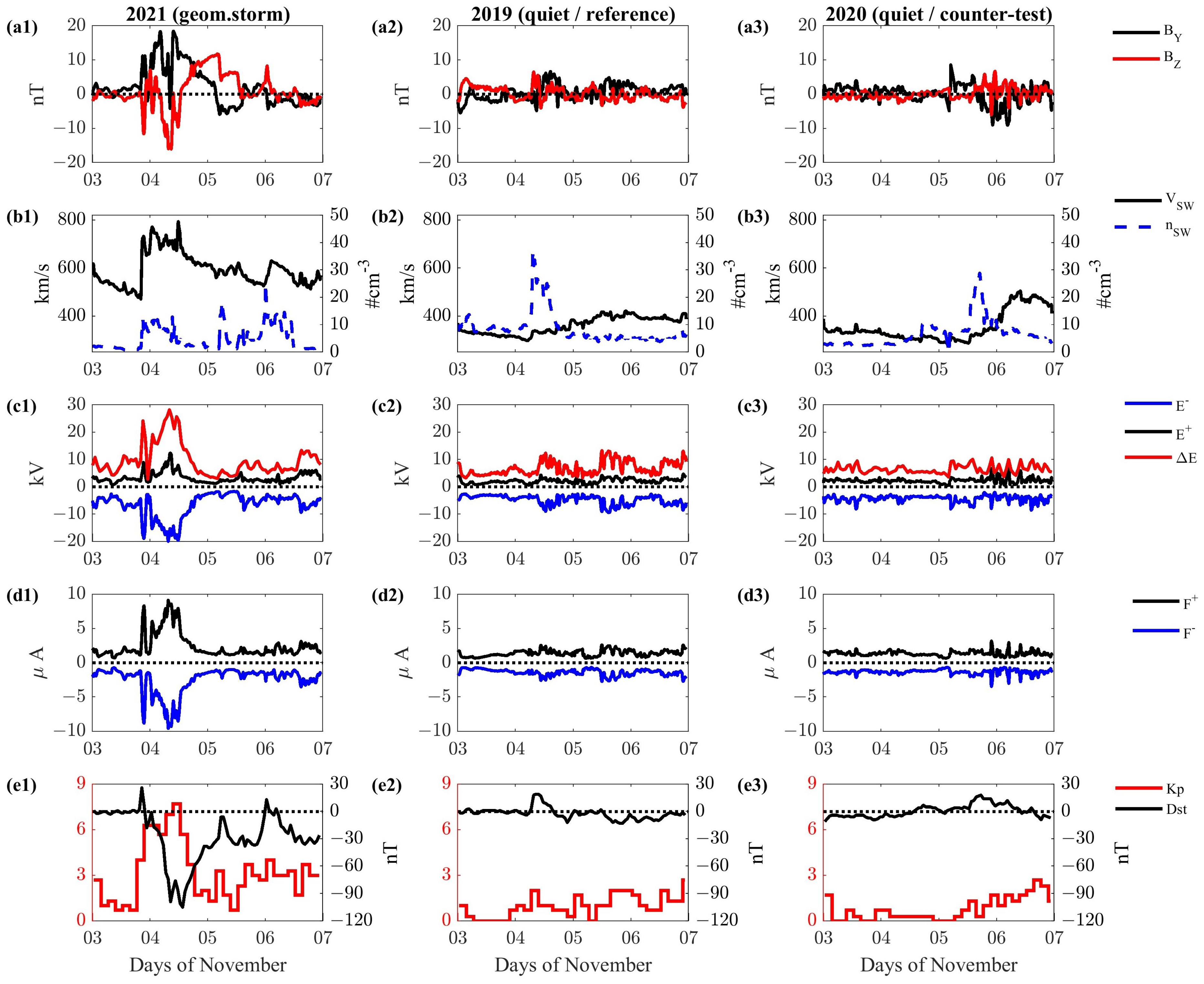
2.1. Solar Wind and Interplanetary Magnetic Field Data

In this work, we aim to reproduce the polar cap electrodynamics through an empirical model since in the high-latitude regions, the solar wind transfers its energy to Earth’s environment more efficiently. Several polar cap electrodynamics climatological models have successfully been used in the past [18,19,20], and also, recently, radar-based models were developed [21,22]. As pointed out by Orr et al. [23], who compared different models in their work, they found that the electric potential and field parameters from the spacecraft-based models have a significantly higher magnitude than the SuperDARN-based models. Nevertheless, the Weimer (W05) model provides reliable information on the polar cap electrodynamics and was successfully applied for searching for the correspondence between high-latitude developed structures and their ionospheric and thermospheric variability that occurred during recent geomagnetic storms [17,24,25]. This model was developed by using the Spherical Cap Harmonic Analysis (SCHA, [26]) on ionospheric measurements and by relating them with the solar wind parameters, which were used as inputs for the model. Therefore, we believe that the W05 model is suitable for studying the polar cap electrodynamics conditions. It provides the Field-Aligned Current (FAC) intensities, polar cap electric potential, and Joule heating at the ionospheric height. In this regard, we use SW and interplanetary magnetic field (IMF) measurements that are time shifted to the bow shock nose, provided by CDAWeb (available online: https://cdaweb.gsfc.nasa.gov/, accessed on 11 June 2024) at a 5 min time resolution. According to the W05 model, we perform a 45 min (9 samples) moving average, with a step size of 5 min (1 sample), SW velocity $V_{SW}$ and density $n_{SW}$, and the interplanetary magnetic field components $B_Y$ and $B_Z$ (in the GSM reference system). We compute the W05 model outputs for each time interval by considering the geographic latitudes $\Phi$ and longitudes $\lambda$ in the range $50°<|\Phi |<90°$ and $-180°<\lambda <180°$, respectively, by defining a regular grid with latitudinal and longitudinal resolutions of ∼2° and ∼4.5°, respectively. Then, for a practical purpose, the W05 outputs are averaged over the entire cap, hereafter indicated with the term hemispheric average, leading to time-dependent quantities that are hereafter indicated as J, E, and F for Joule heating, polar cap electric potential, and FACs intensity, respectively. Regarding E and F, we find it useful to distinguish positive and negative contributions associated with distinct regions (positive and negative cells) to better highlight the evolution of the storm: specifically $E^{+}$ ($E^{-}$) refers to the positive (negative) hemispheric average of electric potential, while $F^{+}$ ($F^{-}$) refers to the positive (negative) hemispheric average of FACs intensities. This choice allows us to compute useful quantities, derived from the W05 model, such as $\Delta E=E^{+}-E^{-}$, which can be regarded as a proxy of the polar cap potential difference, and the total FAC intensity $F_{tot}=F^{+}-F^{-}$.

2.2. Atmospheric Data

To study the space weather effect on the atmosphere, we use data from the ERA5 archive. ERA5 [27,28] is the fifth-generation reanalysis of the global climate by the European Centre for Medium-Range Weather Forecasts (ECMWF, available online: https://www.ecmwf.int/, accessed on 11 June 2024) atmospheric model, covering the period from January 1940 to the present, and is produced within the Copernicus Climate Change Service (C3S; [29], accessed on 11 June 2024). ERA5 provides hourly estimates of many atmospheric, land, and oceanic atmospheric variables. The data cover the Earth on a 30 km horizontal grid and resolve the atmosphere using 137 (hybrid sigma pressure) levels from the surface up to a height (hereafter indicated as h) of 80 km. Atmospheric data are directly available also as interpolated to 37 pressure or 17 potential temperature levels. ERA5 combines vast amounts of historical observations into global estimates using advanced modeling and data assimilation systems. The much higher temporal and spatial resolutions than those of previous available global reanalyses allow for a detailed evolution of weather systems. For this study, we focus on pressure level variables, such as temperature (T), specific humidity (Q), and zonal $(U$) and meridional (V) wind velocity components.

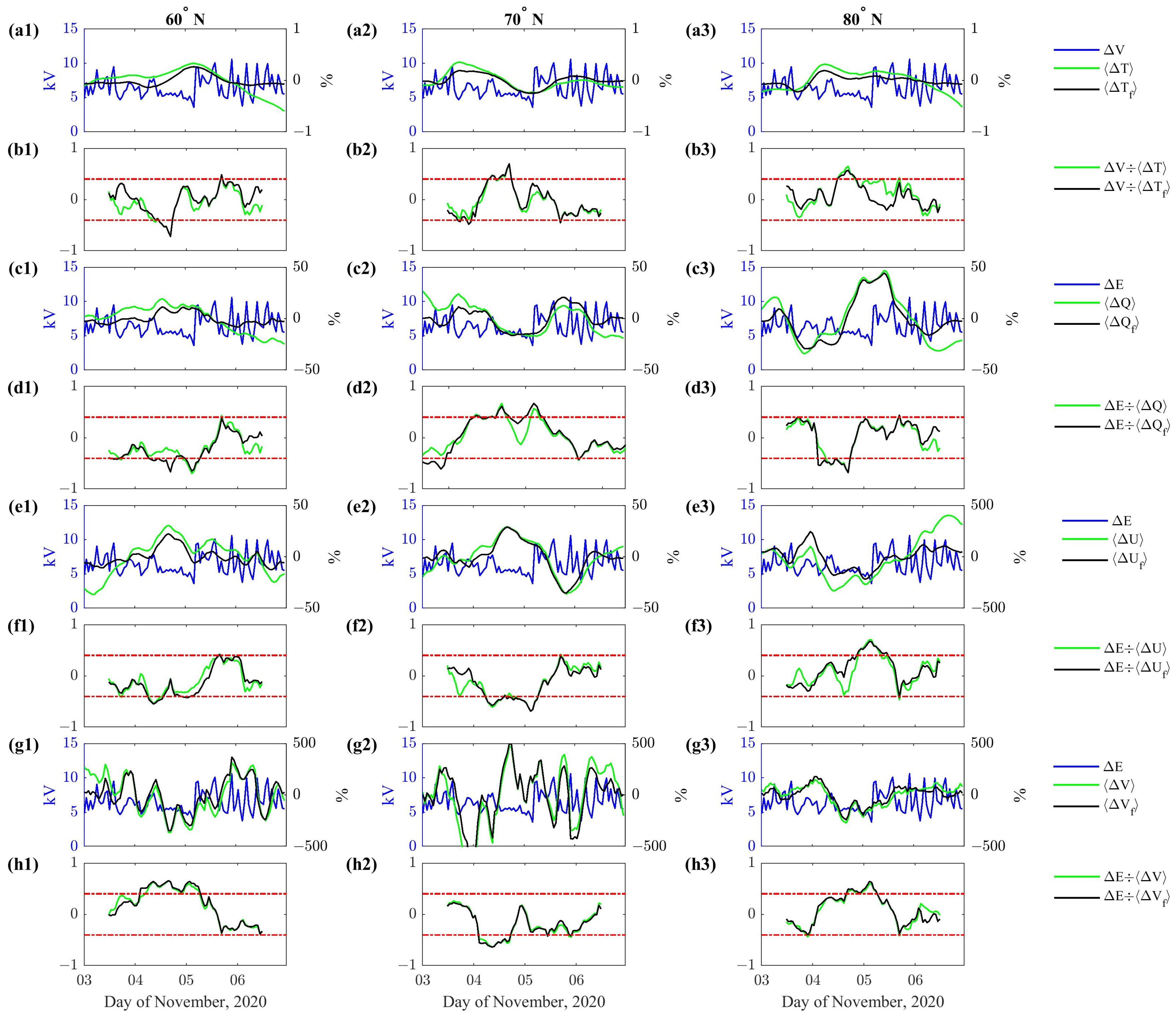
2.3. The Relationship between SW and Atmospheric Parameters

We investigate the correlation between SW and zonally averaged (i.e., the average at all longitudes) atmospheric parameters during 3–6 November 2021. The Pearson correlation r is computed between the assumed input signals computed by the W05 model and the atmospheric parameters. The analysis is performed at all latitudes and heights. To investigate the response of the atmospheric parameters to the polar cap electrodynamic activity enhancement, we compare their variations during the geomagnetically disturbed time interval to a quiet time frame. We use as a reference time interval the same days of the disturbed period but during the nearest quiet year. Furthermore, we also perform a counter-test analysis by using the same methods but choosing as the time interval of the investigation another nearest year characterized by low geomagnetic activity.

Figure 1 shows the interplanetary parameter conditions, the hemispheric average $E^{+}$, $E^{-}$, $F^{+}$, and $F^{-}$ of electrodynamics parameters obtained by the W05 model, and the geomagnetic activity indices disturbance storm time (Dst) and Kp during 3–6 November for the three selected years: 2019, 2020, and 2021. The estimated electrodynamics activity levels are mainly reached during the geomagnetic storm time interval, i.e., from the end of 3 November to the whole day of 4 November 2021, with a consequent increase in the geomagnetic activity indices. Conversely, during the same days of November but for the years 2019 and 2020, the interplanetary conditions are not favorable for an increase in geomagnetic activity as predicted by the W05 model and confirmed by geomagnetic activity indices. In particular, the lowest geomagnetic activity level is reached during the same days of November 2019, which we choose as the reference year, while 2020 is chosen for the counter-test analysis. Based on these observations, we define the relative percentage deviation of a selected zonally averaged atmospheric parameter during the disturbed geomagnetic condition X, with respect to the same assimilated atmospheric parameter during the reference period $X_0$ as follows:

$$\Delta X(\%)={\displaystyle \frac{(X-X_0)}{X_0}}\times 100$$

(1)

where X represents the zonal mean atmospheric parameter (T, Q, U or V), while $X_0$ is computed as the time average of the zonal mean parameter during 2019.

3. Results

In this section, we present the results of our investigations. The correlation analyses among SW-driven polar cap dynamic variations and atmospheric parameters are shown in Section 3.1: it reports the relative deviations during the 3–6 November geomagnetic storm and, for comparison, what was found by the counter-test analysis during the same time interval in 2020 and for both the hemispheres. In the next Section 3.2, we report the investigation of the possible effect of the SW turbulent state in Joule heating phenomena in polar regions.

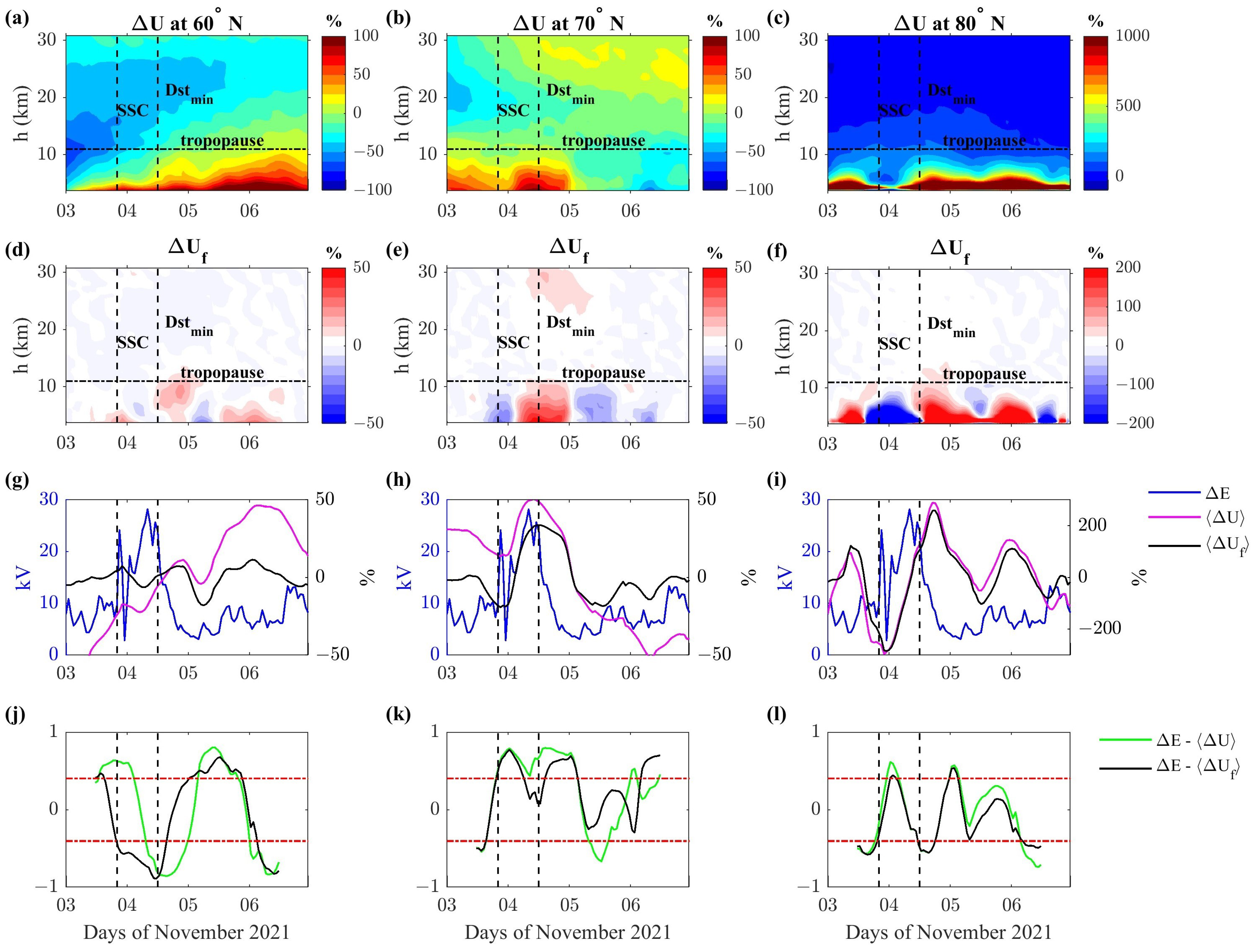
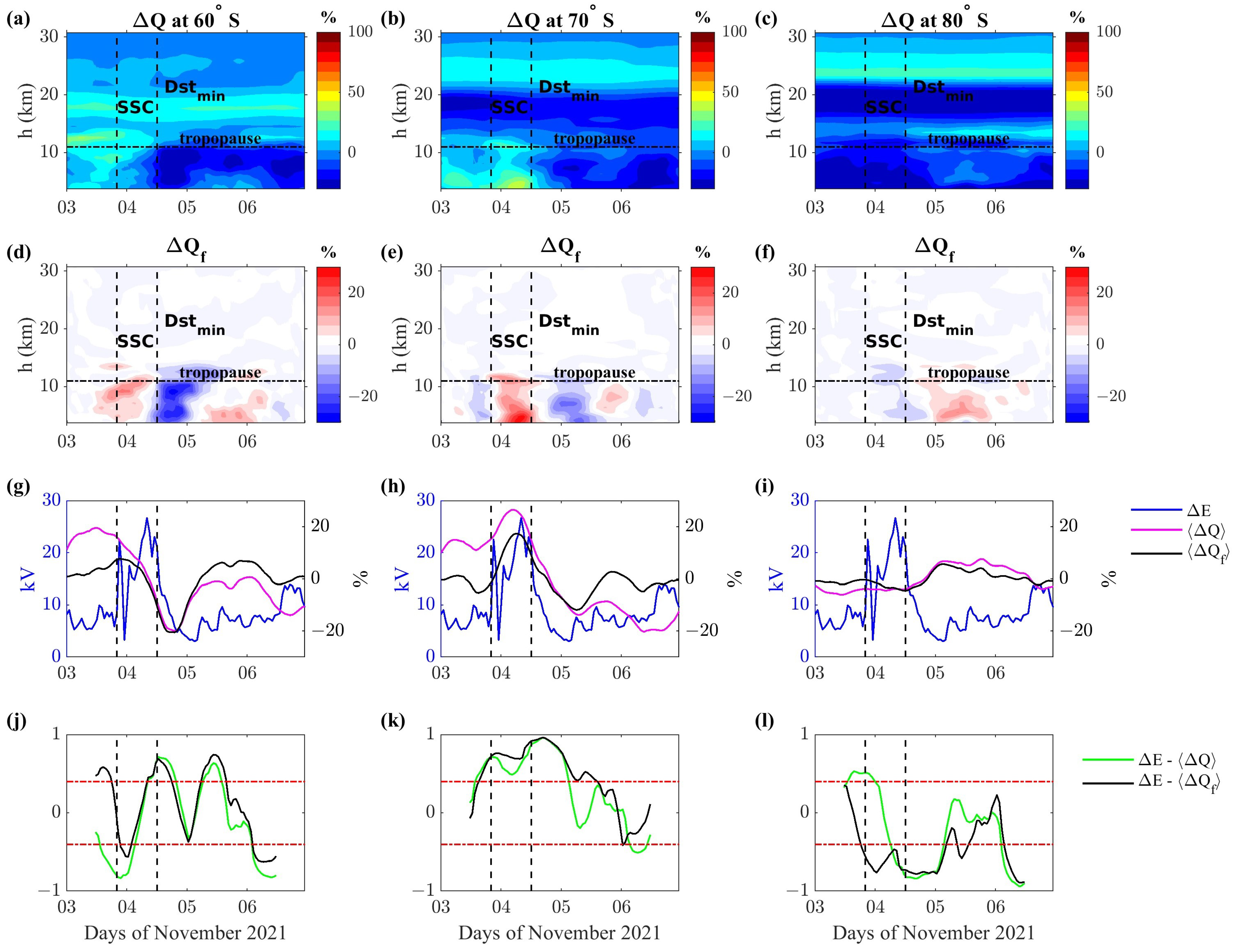
3.1. Changes in Tropospheric and Stratospheric Parameters during the Geomagnetic Storm

Figure 2a–c show the relative deviation in temperature $\Delta T$ during the disturbed period of November 2021 at three different latitudes 60°, 70°, and 80°N, in the northern hemisphere. From these panels, it is not clear how the temperature may be influenced by the geomagnetic activity, here marked by vertical bars in correspondence of the Storm Sudden Commencement (SSC) and the minimum of the Dst. It is a matter of fact that troposphere and stratosphere systems show important differences in terms of dynamics, vertical temperature gradient and stability, ozone content and chemistry, the abundance of moisture, and the presence of clouds. These differences can significantly impact the correlation between SW and atmospheric parameters at different altitudes.

To better study these aspects, we first focus our investigations on the troposphere by calculating the vertical average $\Delta T$ over 3–11 km (the tropopause indicative altitude is chosen approximately at 11 km), indicated as $〈\Delta T〉$, shown as magenta curves in Figure 2g–i; then, we compute the correlation among $〈\Delta T〉$ and $\Delta E$ estimated by W05 model. Due to the large variability in both $\Delta E$ and $〈\Delta T〉$, we prefer to compute a moving correlation $r\left(t\right)$ by considering a moving time window of 24 h with a step size of 1 h (t represents the time at the center of each time window). The results are shown as green lines in Figure 2j–l. The correlations are compared with the threshold at the 5% confidence level obtained (red horizontal lines) from the null hypothesis, based on the actual degree of freedom (DoF) of 24 samples. It can be seen that significant and high values of $\left|r\right(t\left)\right|$ are reached during the geomagnetic storm, from the SSC to the recovery phase, although fluctuating, probably attributable to the long-term trends in $〈\Delta T〉$, absent in $\Delta E$. In particular, we observe an anticorrelation at 60°N and a correlation at higher latitudes of 70° and 80°N. A better result is obtained by high-pass filtering $〈\Delta T〉$: in this regard, we remove from $\Delta T$ its longer periodicities (>4 days) identified through a moving average procedure (e.g., [17,30]); this long-period component is then subtracted to the original dataset. Figure 2d–f show the filtered time series $\Delta T_f$ for each altitude; it shows more clearly the variability during the geomagnetic storm at tropospheric and stratospheric (perhaps less clear) heights. In a separate analysis, we compute the filtered altitude average $〈\Delta T_f〉$ and the altitude average $〈\Delta T〉$, here indicated by ${〈\Delta T〉}_f$. Since these quantities are very similar, we use $〈\Delta T_f〉$ for our investigations (black curves in Figure 2g–i). The corresponding moving correlation among $〈\Delta T_f〉$ and $\Delta E$ emerges more from the uncertainty region and stays up longer than the correlation among $〈\Delta T〉$ and $\Delta E$, especially during the geomagnetic storm main phase. With the same methodology, we compute the relative deviation of specific humidity $\Delta Q$, zonal wind $\Delta U$, and meridional wind $\Delta V$ for the same time interval 3–6 November 2021. The results are shown in Figure 3, Figure 4 and Figure 5 for $\Delta Q$, $\Delta U$, and $\Delta V$, respectively.

Regarding $\Delta Q$ shown in Figure 3, it is evident that major deviations are observed in the troposphere, where Q values are higher than in the stratosphere. In particular, $|\Delta Q_f|$ reaches ∼30% in the troposphere; it also shows a weak increase with increasing latitude (panels d–f), with higher absolute correlation values between $〈\Delta Q_f〉$ and $\Delta E$ at 70°N (panel k, black line). Again, according to what is found with the temperature (Figure 2), we observe an anticorrelation at 60°N and a correlation at higher latitudes. Regarding the horizontal velocities, $\Delta U$ is the only one showing a relationship with $\Delta E$. In the troposphere, $\Delta U$ seems to increase with increasing latitudes, i.e., the opposite with respect to $\Delta Q$ (see Figure 3 and Figure 4). However, the correlation between $〈\Delta U_f〉$ and $\Delta E$ (panels j–l) seems lower than that found for previous parameters. To further support and verify the link between geomagnetic activity and atmospheric parameters, we show the results of the counter-test analysis in Figure 6 for the relative deviations of T, Q, U, and V; the procedure used is the same for generating Figure 2, Figure 3, Figure 4 and Figure 5 but for 3–6 November 2020, always using 2019 as a reference. For simplicity, we report only the investigations conducted by considering the northern hemisphere. It can be seen that the correlation between $\Delta E$ and $\Delta X$ is very low (see Figure 6, panels b1–b3, d1–d3, f1–f3, and h1–h3) for all the atmospheric parameters here considered. Therefore, we conclude that the atmospheric parameter deviations are not related to $\Delta E$ during quiet periods.

The same correlation analysis is conducted for the southern hemisphere. The results are reported in Figure 7, Figure 8, Figure 9 and Figure 10. Again, by comparing the filtered relative variations of atmospheric parameters in the troposphere with $\Delta E$, in the southern hemisphere, we find a remarkable correlation, except for the meridional velocity V. Looking at panels j–l in Figure 2, Figure 3 and Figure 4 and Figure 7, Figure 8 and Figure 9, it also seems that a time delay between the polar cap potential difference increase and the atmospheric parameters increase (correlation) or decrease (anticorrelation) exists, while the time delay for $\Delta V$ is not clear (see Figure 5 and Figure 10. To better investigate the links between geomagnetic activity and atmospheric parameters, we perform a cross-covariance analysis between $\Delta E$ and $\Delta X_f$. To investigate the atmospheric response at all altitudes, also increasing the height resolution of correlation analysis, thereafter we compute the height-averaged $〈\Delta X_f〉$ in the whole atmosphere by selecting strata from 0 to 35 km with a thickness of 5 km and a step size of 1 km. The cross-covariance $r(\Phi ,h,\tau )$, computed between $\Delta E$ and $〈\Delta X_f〉$, here investigated is defined as a function of $\Phi$, height h, and time lag $\tau$: hereafter, negative lags mean that the input $\Delta E$ precedes the output $\Delta X$. It is a matter of fact that the geomagnetic activity varies with the geomagnetic coordinates, while the atmospheric parameters are referenced to geographic ones; in addition, since it is not known a priori if the possible effect of $\Delta E$ increases or decreases the corresponding atmospheric parameter, we consider the absolute value of the correlations. With this choice, the calculated correlation is high when the geomagnetic activity leads the atmospheric parameter regardless of its increase or decrease. Therefore, it is useful to evaluate the averaged absolute value of cross-covariance on all $\Phi$ and h as follows:

$$R\left(\tau \right)={\displaystyle \frac{1}{N}}\sum _{\Phi ,h}\left|r(\Phi ,h,\tau )\right|$$

(2)

where N represents the actual DoF, i.e., the number of points ($\Phi$,h). We perform a MC test for computing significance levels of R (e.g., [12]). In this regard, the 99% confidence threshold is computed by generating 10,000 uncorrelated pairs of time series $\Delta E$ and $〈\Delta X_f〉$, each one reproducing the corresponding actual spectral slope characterized by red noise. The red noise is realized by considering the actual first-order autoregressive AR(1) process of both time series, obtained from the autocorrelation coefficient at lag = 1. For a complete discussion, see [31]. In the MC test, the value of N depends on the strata investigated: by considering the whole atmospheric strata, N is equal to 630 (21 latitudes and 30 levels), independently of the hemisphere and time delay. To better investigate the effects at tropospheric ($3<h<11$ km) and stratospheric ($h>11$ km) heights, different DoFs are considered: 168 and 462 points for troposphere and stratosphere, respectively.

The resulting $R\left(\tau \right)$ is reported in Figure 11, in both the hemispheres and stratospheric and tropospheric heights, together with the confidence threshold at 99% and for all the examined assimilated datasets (black curves). For completeness, we also report the results obtained for the counter-test (gray curves: quiet periods). It is clear that during the 3–6 November 2021, $\Delta E$ is significantly correlated with all the filtered averaged relative variations $〈\Delta T_f〉$, $〈\Delta Q_f〉$, and $〈\Delta U_f〉$, at both tropospheric and stratospheric heights and in both the hemispheres (the black curves well exceed the corresponding thresholds). Regarding $〈\Delta V_f〉$, the correlation is generally lower with respect to that found for the other parameters; in particular, it is slightly correlated with $\Delta E$ only at tropospheric heights, with lower values in the southern hemisphere, while at stratospheric heights, it seems to be unaffected by the geomagnetic activity. In all cases examined here, the maximum correlation values are reached at negative lags, consistent with the hypothesis that geomagnetic activity leads to changes in atmospheric parameters. Conversely, during 3–6 November 2020 (the counter-test analysis), no parameter is related to the corresponding low geomagnetic activity in both the hemispheres and in the troposphere and stratosphere.

Table 1. The results of cross-covariance analysis between $〈\Delta X_f〉$ and $〈\Delta E〉$ in both the northern and southern hemispheres and for the whole atmosphere, the stratosphere, and the troposphere.

		Northern Hemisphere				Southern Hemisphere
	Param	${\mathit{R}}_{\mathit{max}}$	${\mathit{R}}_{\mathbf{99}\%}$	$\Delta {\mathit{R}}_{\mathit{rel}}$	$\mathit{\tau }$ (h)	${\mathit{R}}_{\mathit{max}}$	${\mathit{R}}_{\mathbf{99}\%}$	$\Delta {\mathit{R}}_{\mathit{rel}}$	$\mathit{\tau }$ (h)
Atmosphere (troposphere + stratosphere)	T	0.45	0.27	0.7	−9	0.42	0.26	0.6	−15
	Q	0.43	0.27	0.6	−11	0.43	0.26	0.7	−16
	U	0.44	0.27	0.6	−13	0.36	0.26	0.4	−14
Stratosphere	T	0.45	0.22	0.6	−9	0.45	0.22	0.7	−24
	Q	0.44	0.22	0.6	−12	0.42	0.22	0.6	−16
	U	0.45	0.22	0.7	−14	0.37	0.22	0.4	−28
Troposphere	T	0.46	0.20	0.7	−10	0.41	0.21	0.7	−25
	Q	0.45	0.20	0.6	−7	0.46	0.22	0.8	−16
	U	0.44	0.23	0.6	−11	0.38	0.20	0.7	−28

summarizes the main results of the cross-covariance analysis by reporting the maximum value of correlation $R_{max}$, the corresponding time delay $\tau \left(R_{max}\right)$, and the 99% confidence threshold $R_{99\%}$, where $R_{max}$ is the correlation value that exceeds the corresponding threshold of 20%; please note that with this choice, for example, the correlation peak at the positive lag in $\Delta U$ (in the southern troposphere) is not considered. For completeness, the entire atmospheric column is analyzed.

It appears clear from these analyses that the highest correlation levels are obtained, both for the stratosphere and the troposphere, at negative lags, i.e., consistently with the hypothesis that the geomagnetic activity leads to atmospheric parameter variations. Specifically, in the northern hemisphere, the maximum correlations are attained within 24 h, while in the southern hemisphere they are attained up to ∼28 h. In addition, the lags are greater in the southern stratosphere with respect to the northern one; the same is observed by considering the entire atmospheric column (Table 1). Less clear results are found for $\Delta V$, which seems not to be significantly influenced by polar cap electrodynamics in both hemispheres. Cross-covariance analysis results suggest that, during the 3–4 November 2021 geomagnetic storm, the SW energy transfer to the atmosphere is faster in the northern hemisphere.

Previous investigations conducted by Regi et al. [11] show a clear latitudinal dependence of coherence between the geomagnetic activity and the temperature in the southern hemisphere. For comparison with the results of Regi et al. [11], we extend the moving correlation analysis to the whole latitudinal ranges and for both the southern and northern hemispheres. In this regard, the moving correlation depends on the latitude, height, and time, where the assigned time instant is calculated as the mid-time of the moving window. Then, we compute the latitudinal dependence of the correlation between the geomagnetic activity and atmospheric parameters. In this regard, we focus our attention on the time interval between the geomagnetic storm onset, identified by the SSC occurred at ∼20:00 UT on 3 November 2021, and the end of the main recovery phase of the geomagnetic storm, approximately at the end of 5 November 2021. This comparative investigation is conducted by using only $\Delta T$. The latitudinal dependence of the absolute value of the correlation ($r_{\Phi }$) is obtained as follows: (a) for each latitude, we compute the height average of the moving correlation for the troposphere and stratosphere, respectively; (b) the absolute value of the resulting height-average correlation at point (a) for the troposphere or stratosphere is then time averaged in the above-mentioned time interval. In this computation, we consider the time series without time lag. The result is shown in Figure 12 for both the northern and southern hemispheres, together with the thresholds obtained from the MC test on 1000 uncorrelated time series. Regarding the troposphere, it appears clear that the correlation attains higher and reliable values at latitudes higher than ∼65°. In the stratosphere, the situations are very different in the two hemispheres: the higher values are in the north, with the same latitudinal dependence observed in the troposphere; in the southern hemisphere, the correlations are lower with respect to the northern hemisphere and do not show the same latitudinal dependence observed for the troposphere. In both hemispheres (more clearly in the northern one), it seems evident that there is a maximum correlation around the geographic latitude of 75°, which approximately corresponds to the average latitude of the auroral electron flux maximum predicted through the empirical model of Zhang and Paxton [32] by considering the 3 h geomagnetic activity index Kp for the whole time interval of 3–6 November 2021.

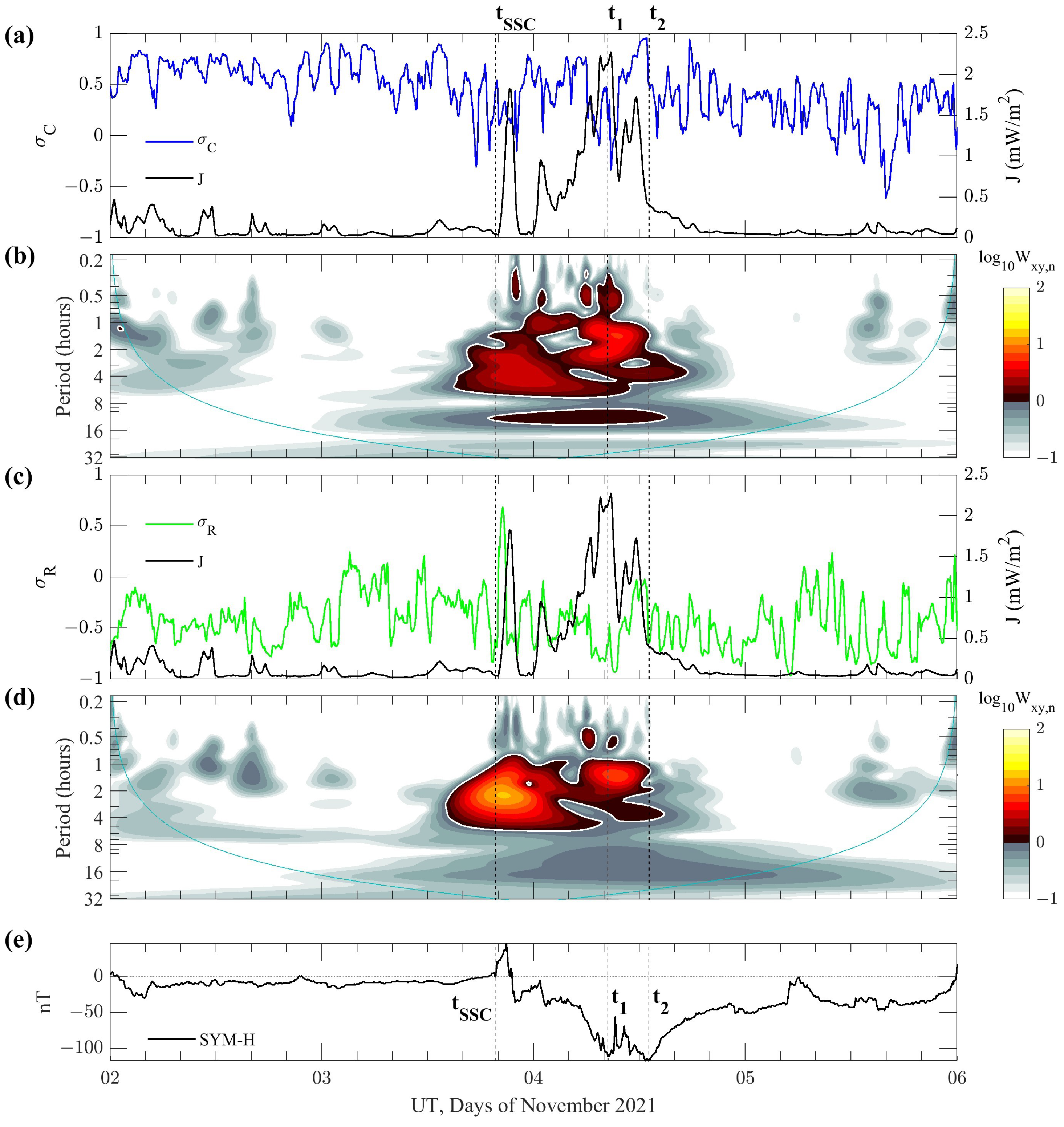
3.2. On the Possible Link between Solar Wind Turbulence with Joule Heating

As performed in Weimer [19] and Hartinger et al. [33], the magnetic (FAC) and electric potential models can be utilized to compute the Joule heating in the ionosphere, due to the solar wind–magnetosphere–ionosphere interaction. Joule heating is considered an important damping process for the ULF waves [33,34,35,36], which are a source of electric field variability in the ionosphere.

In this section, we investigate the possible relation between ULF wave properties in the SW and the ionospheric Joule heating at high latitudes computed using the W05 empirical model. We are aware that the W05 model does not consider the Joule heating contributions due to magnetotail phenomena; nonetheless, the purpose of this work is mainly to investigate the connections between the variations in the SW/IMF conditions with those in the atmospheric parameters. In this model, the Joule heating is mainly due to the large-scale dissipation current systems caused by plasma transport in the magnetosphere. The W05 is based on time-averaged SW parameters, which corresponds to assuming that the global electric potential is static for timescales greater than 30 min (in this work we performed a 45 min average); therefore, smaller variations are not included when computing the electric potential and, as a consequence, the Joule heating rate.

On the other hand, a useful way to identify the character of the ULF waves in the SW is to study them through adiabatic invariants, in particular, the normalized cross-helicity (${\sigma }_C$) and the normalized residual energy (${\sigma }_R$) computed via Elsässer variables (as in [37,38,39]) using a 1 h moving time window, with a step size of 1 min. We expect Alfvén waves for ${\sigma }_C\to \pm 1$ and ${\sigma }_R\to 0$, and compressional waves or a mixture of Alfvén and compressional waves otherwise. We are interested in comparing the two adiabatic invariants with J that have 1 and 5 min time resolution, respectively. Therefore, to make both time series comparable, ${\sigma }_C$ and ${\sigma }_R$ are resampled at the 5 min time resolution, after the pass-band filter procedure [40]. In addition, in this section, to better identify the time of the beginning of SSC and the time/s of the minimum/a of the geomagnetic storm main phase, we compare them with SYM-H [41] at a 5 min time resolution (Figure 13e). Panel a (c) of Figure 13 shows the normalized cross-helicity (normalized residual energy) in blue (green) and the hemispheric average Joule heating J in black during the geomagnetic storm. We verify that J in both hemispheres are very similar to each other; therefore, for simplicity, we use the J in the northern hemisphere. Only in this section, we chose to restrict the studied time interval to 2–5 November because, in a separate analysis, we do not find any interesting results on day 6. In addition, we include day 2 before the main phase of the geomagnetic storm to have an undisturbed period to compare. A dozen hours before the storm, the SW is in a turbulent state, where the normalized cross-helicity (${\sigma }_C$) exceeds values of 0.8. About 5 h before the SSC and in correspondence with the initial phase of the storm, ${\sigma }_C$ undergoes a large reduction, reaching values close to zero, denoting a lack of correlation between velocity and magnetic fluctuations. Just after the SSC, the normalized residual energy (${\sigma }_R$) (typically slightly negative in the turbulent SW) becomes positive with a peak at 0.6, which denotes a sharp increase in kinetic energy at the expense of the magnetic energy, and the Joule heating suddenly increases. After the SSC, the main phase of the storm is characterized by a new increase in ${\sigma }_C$, between ∼23 and ∼06 UT of 3–4 November, which, however, remains confined between 0.5 and 0.8 and then decreases again toward zero a few hours before the first minimum of the SYM-H (at 08:25 UT on 4 November, indicated with $t_1$). The main phase is therefore characterized by a mixture of both Alfvénic and compressive fluctuations, and the Joule heating reaches a local maximum (∼21 UT on 3 November) in correspondence with compressive waves with a prevalence of kinetic energy (${\sigma }_R>0$) immediately after the SSC. In correspondence with $t_1$, ${\sigma }_C$ is close to zero, and ${\sigma }_R$ is close to $-1$, denoting the presence of compressional waves with a prevalence of magnetic energy; here, the Joule heating reaches its maximum value. Then, in correspondence with the second SYM-H minimum (at 13:05 UT on 4 November, indicated with $t_2$; see also the minimum of the Dst shown in Figure 1 bottom panel), the normalized cross-helicity (${\sigma }_C$) exceeds the threshold of 0.8 for about 1.5 h, reaching a maximum of 0.93. Here, the normalized residual energy (${\sigma }_R$) is very close to zero as expected for Alfvénic waves. In correspondence with $t_2$, the Joule heating decreases toward lower values. After this point, during the recovery phase of the storm, the SW becomes less Alfvénic, and the Joule heating remains low. From what we see during this geomagnetic storm, there is a maximum of J in correspondence with non-Alfvénic/compressive SW fluctuations, both with a prevalence of kinetic energy (at the first maximum after the SSC) and with a prevalence of magnetic energy (at the second maximum in correspondence with $t_1$).

To inspect time-scales of such correspondence between ${\sigma }_C$ and ${\sigma }_R$ with J, we compute the bias-rectified cross-power spectra $W_{xy}$ [31,42] by using wavelet transforms of x (${\sigma }_C$ or ${\sigma }_R$) and y (J) [43]. We focus on the absolute value of $W_{xy}$, and, according to previous investigations, we also compute the corresponding threshold at 95%, $|W_{xy}{|}_{95}$, through the MC test. The MC test is performed on 1000 surrogates of x-y pairs, uncorrelated time series, by considering the actual AR(1) process of x and y [31,42]. For practical purposes, we define normalized absolute value cross-power spectra $W_{xy,n}=|W_{xy}|/|W_{xy}{|}_{95}$. Only values higher than 1 are taken into account. Panels b and d of Figure 13 show the logarithm of $W_{xy,n}$. Clearly, the higher the energy content at common scales (or periods), the higher $W_{xy,n}$ is, and, in addition, the significant $W_{xy,n}$ values are attained during the time intervals between $t_{SSC}$ and $t_2$, i.e., during the main phase of the storm. This suggests that during the SW–magnetosphere coupling time interval, when magnetospheric convection is active, part of the SW energy as magnetohydrodynamic waves penetrates efficiently up to the ionospheric height. Of course, since J is essentially driven by the convection process, it is not able to take into account the wave effects. However, our investigations, supported via Elsässer variables in the SW, allow us to study the presence of such waves in SW and their possible link with J at the ionospheric height. The electrodynamics of the polar cap exhibits interesting aspects if related to the observed fluctuations in ${\sigma }_C$ and ${\sigma }_R$ at timescales greater than 10 min (because of the 5 min resolution of ${\sigma }_C$, ${\sigma }_R$, and J): the decrease in Alfvénicity (increasing in the compressional fluctuations) around $t_{SSC}$ and $t_1$ corresponds to a J increase, regardless of the prevalence of kinetic or magnetic energy of the compressive fluctuations. In correspondence with $t_2$, we observe the presence of Alfvénic fluctuations in correspondence with a J increase; here, a plausible dissipation of Alfvénic fluctuations in the polar cap currents may occur since, from here on, J attains lower values.

4. Discussion

We study the possible effects of the geomagnetic storm of 3–6 November 2021 on the troposphere and stratosphere. The investigations are regarding both the hemispheres at latitudes greater than $50°$, by using the ERA5 [27,28] atmospheric reanalysis dataset, polar cap potential difference, and Joule heating provided by the W05 model through the SW dataset. The relative (with respect to 2019) atmospheric parameter variations computed in correspondence with the storm (disturbed days) in November 2021 are compared with those computed during the same time interval in November 2020 (quiet days, for counter-test). We also analyze the significance of the correlation analysis between relative atmospheric parameter variations and polar cap potential difference by using the MC test. To verify the hypothesis that the SW leads to atmospheric variations, we analyze the time lag between them via cross-correlation analysis between relative variations in atmospheric parameters and polar cap potential difference. We also compute the latitudinal dependence of the correlation coefficients in order to compare our results with previous investigations. Finally, we compare the presence of Alfvén and compressional waves in the SW with the Joule heating (J) at ionospheric height, estimated for the northern hemisphere by the W05 model.

During the geomagnetic storm time interval, the correlation is significantly high in the troposphere and at selected latitudes of $60°$, $70°$ and $80°$N and S; on the contrary, from the counter-test analysis, the correlations are not significant during the quiet time interval in November 2020. From the correlation analyses, the temperature (T), the specific humidity (Q), and the zonal wind velocity (U) show a clear correspondence with the enhanced geomagnetic activity during the storm. In particular, Q shows higher relative variations with respect to T and U. Conversely, V seems to be not affected by the solar wind–magnetosphere coupling process. These results are in agreement with Regi et al. [12], who showed a reliable relationship between those parameters and geomagnetic activity enhancements. The cross-correlation analysis between relative variations in atmospheric parameters and polar cap potential difference reveals always a negative lag of about 1 day, in agreement with the hypothesis that the SW leads the variations of the atmospheric parameters; on the contrary, no significant correlations are found from the counter-test analysis. These results are also in agreement with [12], who found significant variations in cloud cover, temperature, and specific humidity within 2 days after periods characterized by $Bz<0$. The lower delay (<1 day) in the northern hemisphere, with respect to the southern one, could be related to the presence of the stratospheric polar vortex, i.e., the band of strong westerly winds that forms in both the northern and southern polar stratospheres during the winter season. The latitudinal dependence of the correlation analysis between the temperature and polar cap potential on both hemispheres reveals, in agreement with that previously found by Regi et al. [11], a higher and reliable correlation at high latitudes (>$65°$). An additional result is also found: the maximum correlation is observed around the geographic latitude of $75°$ (except for the southern stratosphere). This result could be due to the polar electrodynamic activity intensification that reaches its maximum below the auroral oval. This result is consistent with that of Pudovkin and Veretenenko [44], who found significant variations in zonal atmospheric pressure during geomagnetic storms at auroral and subauroral zones (see also [45] for a review). Therefore, we conclude that the intensification of the polar cap potential difference can play an important role in the solar wind–atmosphere coupling.

In addition, the comparison between the normalized cross helicity (${\sigma }_C$) and the normalized residual energy (${\sigma }_R$) with J seems to indicate that during the SW–magnetosphere coupling time interval, when the magnetospheric convection is active, J increases. We observe J maxima just after $t_{SSC}$ and before the time corresponding to the first SYM-H minimum ($t_1$), where we find compressive waves in the SW, with a prevalence of kinetic energy in the first case and magnetic energy in the second case. On the contrary, another peak of J is observed just before the time corresponding to the second SYM-H minimum ($t_2$), where the waves in the SW are of an Alfvénic nature. It is possible that during the main phase of the storm (where we observe cross-power enhancements, Figure 13c,d) the magnetohydrodynamic waves can be efficiently transmitted from the SW in the magnetosphere up to the ionospheric height. Here, their dissipation can contribute to an additional Joule heating effect not predicted by the W05 model, with possible effects on the lowest heights up to the mesosphere, thermosphere, and at least the stratosphere.

The investigations indicate that the atmospheric parameters’ response is the same in both the hemispheres, with a time-delay response with respect to the polar cap electrodynamic variations of about 1 day (more delayed for the southern hemisphere). The short time-scale response of the atmosphere to the geomagnetic activity examined in this work is therefore reasonably related to the electric field intensity enhancement and variations during disturbed geomagnetic conditions. Such modifications in high-latitude electric fields could result in an intensification of the vertical current system through the troposphere to the ground in the global electric circuit (GEC) [4,5,6,46,47], which could influence the cloud formation through microphysical processes such as electrofreezing and electron scavenging processes [11,48,49], which in turn can affect atmospheric thermodynamics.

5. Conclusions

The main conclusions can be summarized as follows:

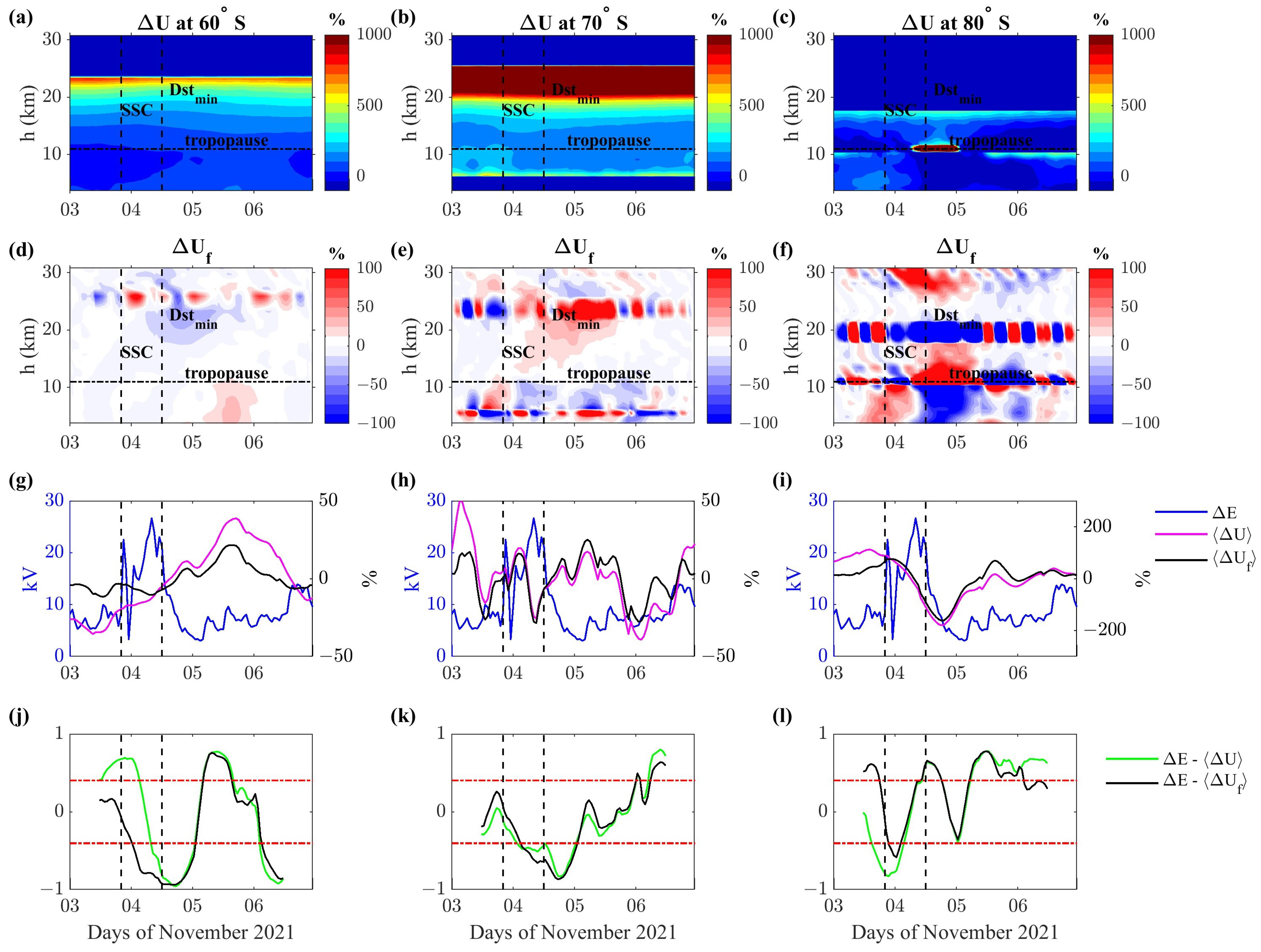
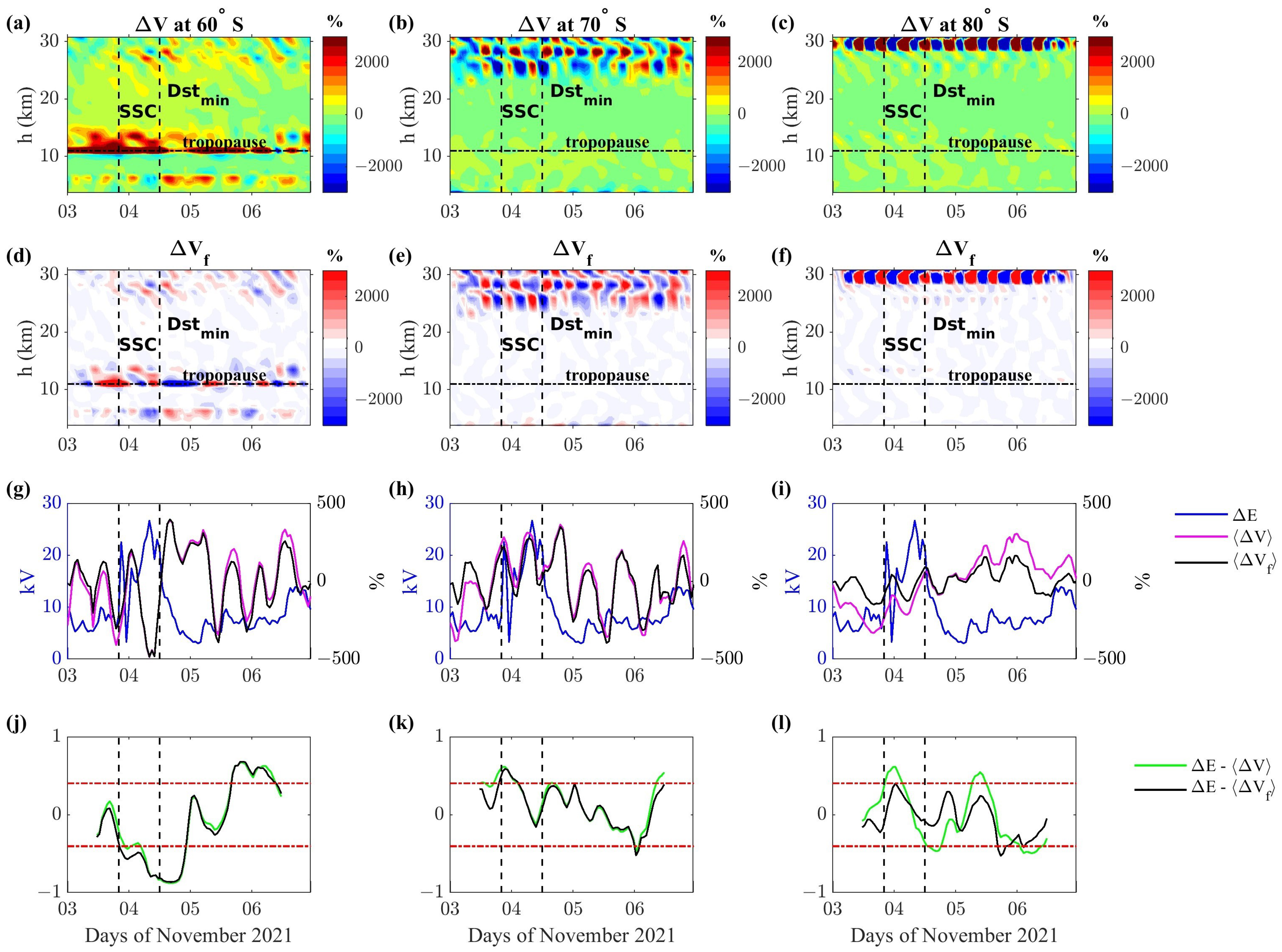
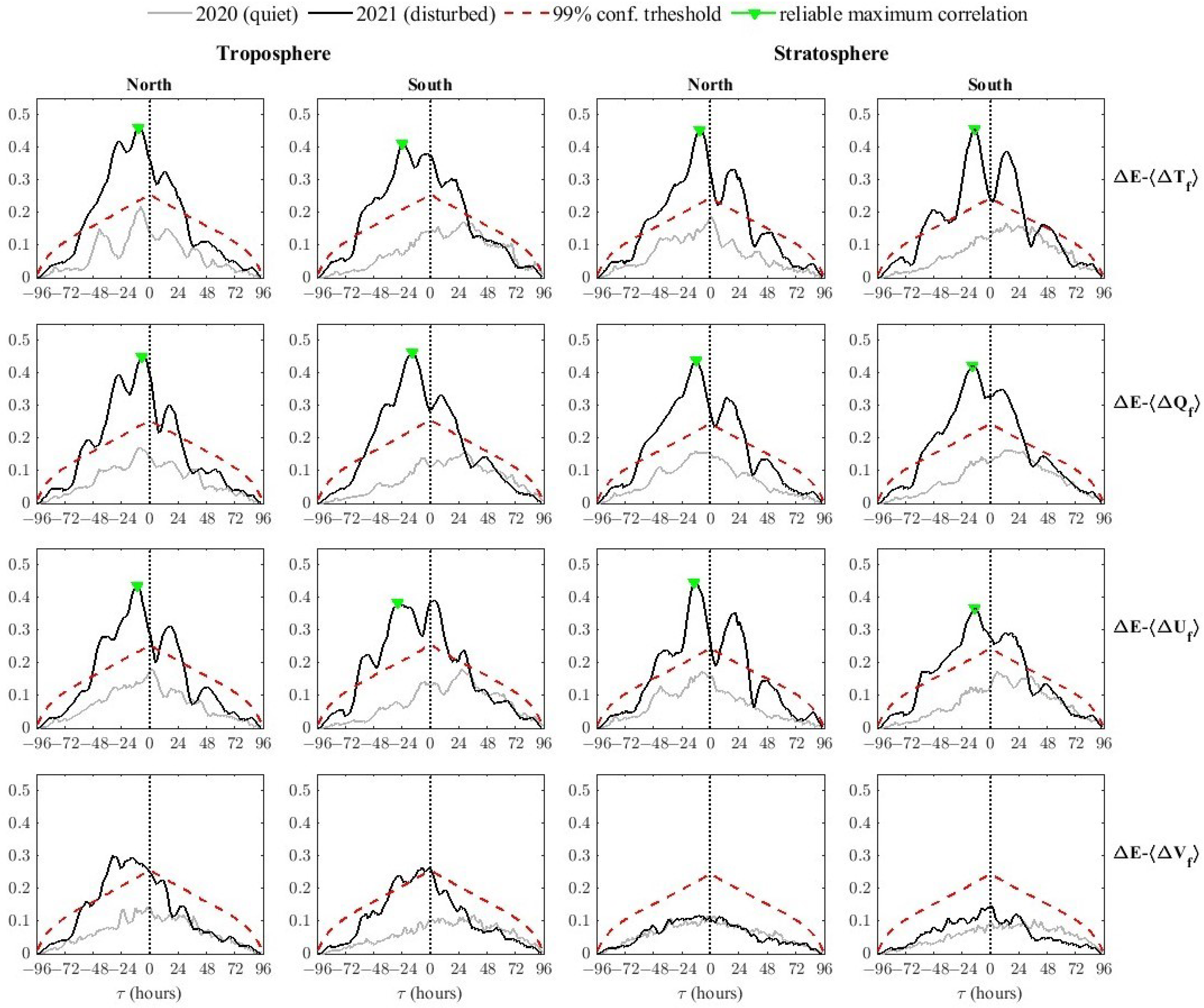
• The atmospheric parameters temperature (T), specific humidity (Q), and zonal wind (U) seem to respond to the solar wind-driven electrodynamics of the polar cap regions and in both the hemispheres during the geomagnetic storm. On the contrary, meridional wind (V) appear unaffected by the solar wind–magnetosphere coupling process.
• The atmospheric parameters T, Q, and U respond approximately within one day to the geomagnetic activity: the shorter delay in the northern hemisphere compared to the southern one may be attributed to the stratospheric polar vortex in the northern hemisphere.
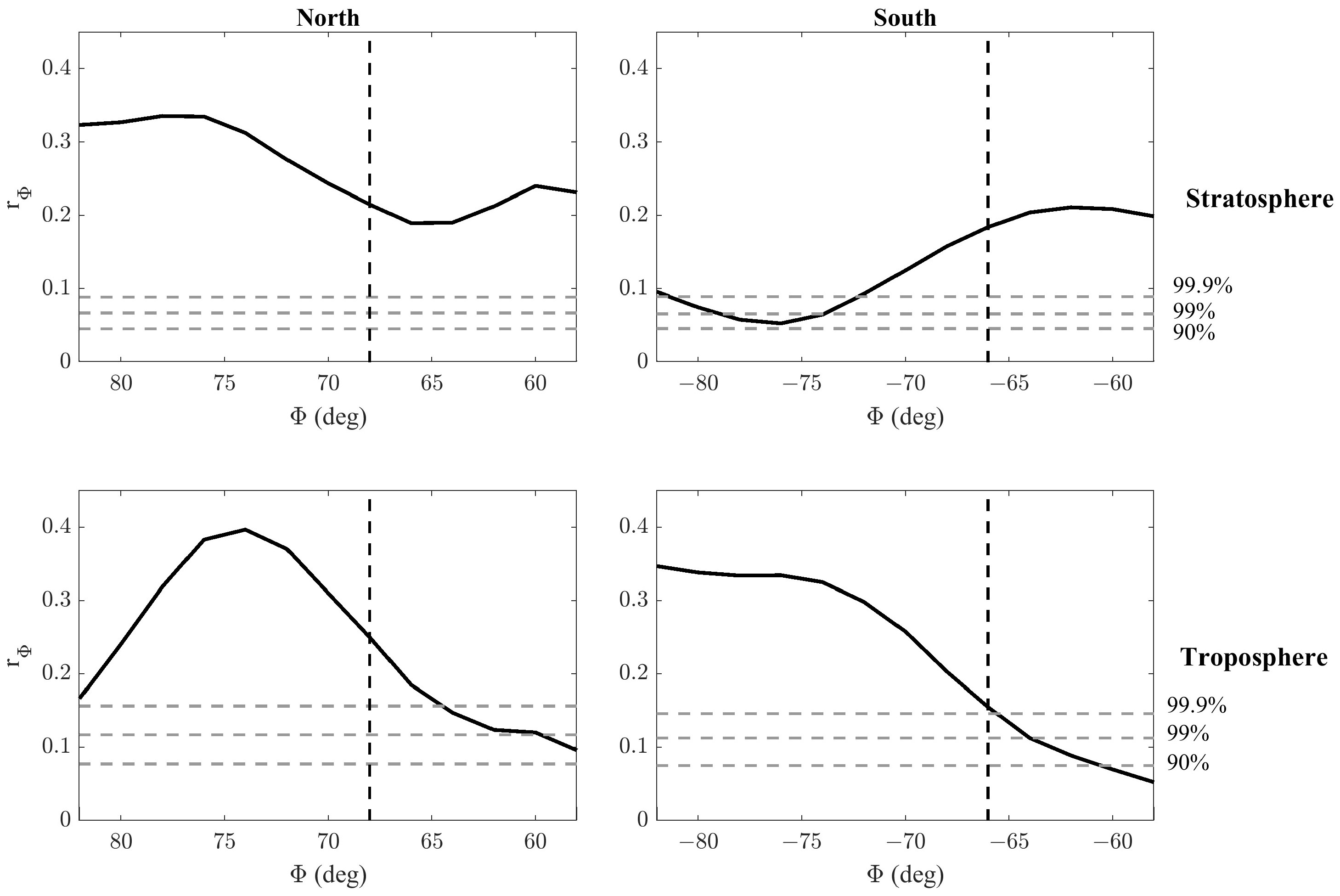
• The latitudinal investigation suggests that the temperature has a major correspondence with the polar cap potential difference near the auroral regions, where the electrodynamic activity, due to solar wind–atmosphere coupling processes, maximizes.
• During the storm’s main phase, the solar wind turbulence state seems to play a role in the transfer of energy from the interplanetary medium into the magnetosphere, in a complex way, causing additional Joule heating effects.

It must be noted that, while our analyses reveal a clear overall correlation between SW and atmospheric parameter variations, suggesting a potential causal relationship consistent with previous literature, a more extensive analysis covering a larger number of cases would be required to establish this robustly. However, such an analysis falls beyond the scope of this paper.

References

1. Yiğit, E.; Knížová, P.K.; Georgieva, K.; Ward, W. A review of vertical coupling in the Atmosphere-Ionosphere system: Effects of waves, sudden stratospheric warmings, space weather, and of solar activity. J. Atmos. Sol.-Terr. Phys. 2016, 141, 1–12. [Google Scholar] [CrossRef]
2. Seppälä, A.; Matthes, K.; Randall, C.E.; Mironova, I.A. What is the solar influence on climate? Overview of activities during CAWSES-II. Eur. J. Nucl. Med. Mol. Imaging 2014, 1, 24. [Google Scholar] [CrossRef]
3. Mironova, I.A.; Aplin, K.L.; Arnold, F.; Bazilevskaya, G.A.; Harrison, R.G.; Krivolutsky, A.A.; Nicoll, K.A.; Rozanov, E.V.; Turunen, E.; Usoskin, I.G. Energetic Particle Influence on the Earth’s Atmosphere. Space Sci. Rev. 2015, 194, 1–96. [Google Scholar] [CrossRef]
4. Tinsley, B.A.; Zhou, L. Initial results of a global circuit model with variable stratospheric and tropospheric aerosols. J. Geophys. Res. Atmos. 2006, 111, D16205. [Google Scholar] [CrossRef]
5. Tinsley, B.A.; Burns, G.B.; Zhou, L. The role of the global electric circuit in solar and internal forcing of clouds and climate. Adv. Space Res. 2007, 40, 1126–1139. [Google Scholar] [CrossRef]
6. Lam, M.M.; Tinsley, B.A. Solar wind-atmospheric electricity-cloud microphysics connections to weather and climate. J. Atmos. Sol.-Terr. Phys. 2016, 149, 277–290. [Google Scholar] [CrossRef]
7. Lei, J.; Thayer, J.P.; Forbes, J.M.; Sutton, E.K.; Nerem, R.S.; Temmer, M.; Veronig, A.M. Global thermospheric density variations caused by high-speed solar wind streams during the declining phase of solar cycle 23. J. Geophys. Res. Space Phys. 2008, 113, A11303. [Google Scholar] [CrossRef]
8. Thayer, J.P.; Lei, J.; Forbes, J.M.; Sutton, E.K.; Nerem, R.S. Thermospheric density oscillations due to periodic solar wind highspeed streams. J. Geophys. Res. Space Phys. 2008, 113, A06307. [Google Scholar] [CrossRef]
9. Jiang, G.; Wang, W.; Xu, J.; Yue, J.; Burns, A.G.; Lei, J.; Mlynczak, M.G.; Rusell, J.M. Responses of the lower thermospheric temperature to the 9-day and 13.5-day oscillations of recurrent geomagnetic activity. J. Geophys. Res. Space Phys. 2014, 119, 4841–4859. [Google Scholar] [CrossRef]
10. Francia, P.; Regi, M.; De Lauretis, M. Signatures of the ULF geomagnetic activity in the surface air temperature in Antarctica. J. Geophys. Res. Space Phys. 2015, 120, 2452–2459. [Google Scholar] [CrossRef]
11. Regi, M.; Lauretis, M.D.; Redaelli, G.; Francia, P. ULF geomagnetic and polar cap potential signatures in the temperature and zonal wind reanalysis data in Antarctica. J. Geophys. Res. Space Phys. 2016, 121, 286–295. [Google Scholar] [CrossRef]
12. Regi, M.; Redaelli, G.; Francia, P.; Lauretis, M.D. ULF geomagnetic activity effects on tropospheric temperature, specific humidity, and cloud cover in Antarctica, during 2003–2010. J. Geophys. Res. Atmos. 2017, 122, 6488–6501. [Google Scholar] [CrossRef]
13. Voiculescu, M.; Usoskin, I.; Condurache-Bota, S. Clouds blown by the solar wind. Environ. Res. Lett. 2013, 8, 045032. [Google Scholar] [CrossRef]
14. Prikryl, P.; Iwao, K.; Muldrew, D.B.; Rušin, V.; Rybanský, M.; Bruntz, R. A link between high-speed solar wind streams and explosive extratropical cyclones. J. Atmos. Sol.-Terr. Phys. 2016, 149, 219–231. [Google Scholar] [CrossRef]
15. Elsner, J.B.; Jagger, T.H. United States and Caribbean tropical cyclone activity related to the solar cycle. Geophys. Res. Lett. 2008, 35, L18705. [Google Scholar] [CrossRef]
16. Todorović, N.; Vujović, D. Links between geomagnetic activity and atmospheric cold fronts passage over the Belgrade region, Serbia. Meteorol. Appl. 2022, 29, e2107. [Google Scholar] [CrossRef]
17. Regi, M.; Perrone, L.; Del Corpo, A.; Spogli, L.; Sabbagh, D.; Cesaroni, C.; Alfonsi, L.; Bagiacchi, P.; Cafarella, L.; Carnevale, G.; et al. Space Weather Effects Observed in the Northern Hemisphere during November 2021 Geomagnetic Storm: The Impacts on Plasmasphere, Ionosphere and Thermosphere Systems. Remote Sens. 2022, 14, 5765. [Google Scholar] [CrossRef]
18. Heelis, R.A.; Lowell, J.K.; Spiro, R.W. A model of the high-latitude ionospheric convection pattern. J. Geophys. Res. Space Phys. 1982, 87, 6339–6345. [Google Scholar] [CrossRef]
19. Weimer, D.R. Improved ionospheric electrodynamic models and application to calculating Joule heating rates. J. Geophys. Res. 2005, 110, A05305. [Google Scholar] [CrossRef]
20. Weimer, D.R. Predicting surface geomagnetic variations using ionospheric electrodynamic models. J. Geophys. Res. 2005, 110, A12307. [Google Scholar] [CrossRef]
21. Thomas, E.G.; Shepherd, S.G. Statistical Patterns of Ionospheric Convection Derived From Mid-latitude, High-Latitude, and Polar SuperDARN HF Radar Observations. J. Geophys. Res. Space Phys. 2018, 123, 3196–3216. [Google Scholar] [CrossRef]
22. Walach, M.T.; Grocott, A.; Milan, S.E. Average Ionospheric Electric Field Morphologies During Geomagnetic Storm Phases. J. Geophys. Res. Space Phys. 2021, 126, e2020JA028512. [Google Scholar] [CrossRef]
23. Orr, L.; Grocott, A.; Walach, M.T.; Chisham, G.; Freeman, M.P.; Lam, M.M.; Shore, R.M. A Quantitative Comparison of High Latitude Electric Field Models During a Large Geomagnetic Storm. Space Weather 2023, 21, e2022SW003301. [Google Scholar] [CrossRef]
24. Spogli, L.; Sabbagh, D.; Regi, M.; Cesaroni, C.; Perrone, L.; Alfonsi, L.; Di Mauro, D.; Lepidi, S.; Campuzano, S.A.; Marchetti, D.; et al. Ionospheric Response Over Brazil to the August 2018 Geomagnetic Storm as Probed by CSES-01 and Swarm Satellites and by Local Ground-Based Observations. J. Geophys. Res. Space Phys. 2021, 126, e2020JA028368. [Google Scholar] [CrossRef]
25. Alfonsi, L.; Cesaroni, C.; Spogli, L.; Regi, M.; Paul, A.; Ray, S.; Lepidi, S.; Di Mauro, D.; Haralambous, H.; Oikonomou, C.; et al. Ionospheric Disturbances Over the Indian Sector During 8 September 2017 Geomagnetic Storm: Plasma Structuring and Propagation. Space Weather 2021, 19, e2020SW002607. [Google Scholar] [CrossRef]
26. Haines, G.V. Spherical cap harmonic analysis. J. Geophys. Res. Solid Earth 1985, 90, 2583–2591. [Google Scholar] [CrossRef]
27. Hersbach, H.; Bell, B.; Berrisford, P.; Hirahara, S.; Horányi, A.; Muñoz-Sabater, J.; Nicolas, J.; Peubey, C.; Radu, R.; Schepers, D.; et al. The ERA5 global reanalysis. Q. J. R. Meteorol. Soc. 2020, 146, 1999–2049. [Google Scholar] [CrossRef]
28. Hersbach, H.; Bell, B.; Berrisford, P.; Biavati, G.; Horányi, A.; Muñoz Sabater, J.; Nicolas, J.; Peubey, C.; Radu, R.; Rozum, I.; et al. ERA5 hourly data on single levels from 1940 to present. Copernicus Climate Change Service (C3S) Climate Data Store (CDS). ECMWF 2023, 147. Available online: https://cds.climate.copernicus.eu/cdsapp#!/dataset/10.24381/cds.adbb2d47?tab=overview (accessed on 11 June 2024).
29. Thépaut, J.N.; Pinty, B.; Dee, D.; Engelen, R. The CoPerniCUS programme and its climate change service. In Proceedings of the IGARSS 2018-2018 IEEE International Geoscience and Remote Sensing Symposium, Valencia, Spain, 22–27 July 2018; Volume 2018, pp. 1591–1593. [Google Scholar] [CrossRef]
30. Regi, M.; Corpo, A.D.; Lauretis, M.D. The use of the empirical mode decomposition for the identification of mean field aligned reference frames. Ann. Geophys. 2016, 59, G0651. [Google Scholar] [CrossRef]
31. Grinsted, A.; Moore, J.C.; Jevrejeva, S. Application of the cross wavelet transform and wavelet coherence to geophysical time series. Nonlinear Processes Geophys. 2004, 11, 561–566. [Google Scholar] [CrossRef]
32. Zhang, Y.; Paxton, L.J. An empirical Kp-dependent global auroral model based on TIMED/GUVI FUV data. J. Atmos. Sol.-Terr. Phys. 2008, 70, 1231–1242. [Google Scholar] [CrossRef]
33. Hartinger, M.D.; Moldwin, M.B.; Zou, S.; Bonnell, J.W.; Angelopoulos, V. ULF wave electromagnetic energy flux into the ionosphere: Joule heating implications. J. Geophys. Res. Space Phys. 2015, 120, 494–510. [Google Scholar] [CrossRef]
34. Crowley, G.; Wade, N.; Waldock, J.A.; Robinson, T.R.; Jones, T.B. High time-resolution observations of periodic frictional heating associated with a Pc5 micropulsation. Nature 1985, 316, 528–530. [Google Scholar] [CrossRef]
35. Glassmeier, K.H.; Volpers, H.; Baumjohann, W. Ionospheric Joule dissipation as a damping mechanism for high latitude ULF pulsations: Observational evidence. Planet. Space Sci. 1984, 32, 1463–1466. [Google Scholar] [CrossRef]
36. Rae, I.J.; Watt, C.E.; Fenrich, F.R.; Mann, I.R.; Ozeke, L.G.; Kale, A. Energy deposition in the ionosphere through a global field line resonance. Ann. Geophys. 2007, 25, 2529–2539. [Google Scholar] [CrossRef]
37. Elsasser, W.M. The Hydromagnetic Equations. Phys. Rev. 1950, 79, 183. [Google Scholar] [CrossRef]
38. Tu, C.Y.; Marsch, E. MHD structures, waves and turbulence in the solar wind: Observations and theories. Space Sci. Rev. 1995, 73, 1–210. [Google Scholar] [CrossRef]
39. Bruno, R.; Carbone, V. The Solar Wind as a Turbulence Laboratory. Living Rev. Sol. Phys. 2013, 10, 2. [Google Scholar] [CrossRef]
40. Bendat, J.S.; Piersol, A.G. Random Data: Analysis and Measurement Procedures, 1st ed.; John Wiley & Sons: Hoboken, NJ, USA, 1971. [Google Scholar]
41. Li, H.; Wang, C.; Kan, J.R. Contribution of the partial ring current to the SYMH index during magnetic storms. J. Geophys. Res. Space Phys. 2011, 116, A11222. [Google Scholar] [CrossRef]
42. Liu, Y.; Liang, X.S.; Weisberg, R.H. Rectification of the bias in the wavelet power spectrum. J. Atmos. Ocean. Technol. 2007, 24. [Google Scholar] [CrossRef]
43. Torrence, C.; Compo, G.P. A Practical Guide to Wavelet Analysis. Bull. Am. Meteorol. Soc. 1998, 79, 61–78. [Google Scholar] [CrossRef]
44. Pudovkin, M.; Veretenenko, S. Variations of the atmospheric pressure meridional profile during a geomagnetic disturbance. Geomagn. Aeron. 1992, 32, 118–122. [Google Scholar]
45. Raspopov, O.M.; Veretenenko, S.V. Solar activity and cosmic rays: Influence on cloudiness and processes in the lower atmosphere (in memory and on the 75th anniversary of M.I. Pudovkin). Geomagn. Aeron. 2009, 49, 137–145. [Google Scholar] [CrossRef]
46. Tinsley, B.A. The global atmospheric electric circuit and its effects on cloud microphysics. Rep. Prog. Phys. 2008, 71, 066801. [Google Scholar] [CrossRef]
47. Rycroft, M.J.; Nicoll, K.A.; Aplin, K.L.; Giles Harrison, R. Recent advances in global electric circuit coupling between the space environment and the troposphere. J. Atmos. Sol.-Terr. Phys. 2012, 90–91, 198–211. [Google Scholar] [CrossRef]
48. Tinsley, B.A.; Heelis, R.A. Correlations of atmospheric dynamics with solar activity evidence for a connection via the solar wind, atmospheric electricity, and cloud microphysics. J. Geophys. Res. 1993, 98, 10375–10384. [Google Scholar] [CrossRef]
49. Francia, P.; Regi, M.; De Lauretis, M. Solar Wind Signatures Throughout the High-Latitude Atmosphere. J. Geophys. Res. Space Phys. 2018, 123, 4517–4520. [Google Scholar] [CrossRef]
Figure 1. (From top to bottom) The interplanetary parameter conditions B Y , B Z (panels a1a3), V S W and n S W (panels b1b3), used by the W05 model; the hemispheric average in the northern hemisphere of polar cap potential E (panels c1c3) and FACs intensities F (panels d1d3) for both positive (black curves) and negative (blue curves) components, as well as the Δ E (red curves). The same quantities for the southern hemisphere are very similar to those shown here and are not reported for simplicity; the geomagnetic activity indices (panels e1e3) Dst (black curves) and Kp (red segments) during 3–6 November for the three years 2019, 2020 and 2021.
Remotesensing 16 03318 g001
Figure 2. Relative temperature deviation Δ T during 3–6 November 2021 (panels ac) and the time-filtered version Δ T f (panels df) as a function of time and height, for three different geographic latitudes in the northern hemisphere: in these panels, the tropopause is indicated by the horizontal line. Electric field potential difference Δ E (blue line in panels gi) and height average Δ T (magenta line) and filtered Δ T f (black line) atmospheric parameters at tropospheric heights. The result of the moving correlation analysis (panels jl) among Δ E with Δ T (green line) and Δ E with Δ T f (black line). The SSC and minimum value of the Dst index are reported in all panels as vertical dashed lines; the considered tropospheric altitude range of 3–11 km in computing Δ T and then Δ T f is marked by horizontal dashed lines in panels (df). Horizontal red lines in panels (jl) represent the 95% confidence interval.
Remotesensing 16 03318 g002
Figure 3. Relative specific humidity Δ Q during 3–6 November 2021 (panels ac) and the time-filtered version Δ Q f (panels df) as a function of time and height, for three different geographic latitudes in the northern hemisphere: in these panels, the tropopause is indicated by the horizontal line. Electric field potential difference Δ E (blue line in panels gi) and height average Δ Q (magenta line) and filtered Δ Q f (black line) atmospheric parameters at tropospheric heights. The result of the moving correlation analysis (panels jl) among Δ E with Δ Q (green line) and Δ E with Δ Q f (black line). The SSC and minimum value of the Dst index are reported in all panels as vertical dashed lines; the considered tropospheric altitude range of 3–11 km in computing Δ Q and then Δ Q f is marked by horizontal dashed lines in panels (df). Horizontal red lines in panels (jl) represent the 95% confidence interval.
Remotesensing 16 03318 g003
Figure 4. Relative zonal wind Δ U during 3–6 November 2021 (panels ac) and the time-filtered version Δ U f (panels df) as a function of time and height, for three different geographic latitudes in the northern hemisphere: in these panels, the tropopause is indicated by the horizontal line. Electric field potential difference Δ E (blue line in panels gi) and height average Δ U (magenta line) and filtered Δ U f (black line) atmospheric parameters at tropospheric heights. The result of the moving correlation analysis (panels jl) among Δ E with Δ U (green line) and Δ E with Δ U f (black line). The SSC and minimum value of the Dst index are reported in all panels as vertical dashed lines; the considered tropospheric altitude range of 3–11 km in computing Δ U and then Δ U f is marked by horizontal dashed lines in panels (df). Horizontal red lines in panels (jl) represent the 95% confidence interval.
Remotesensing 16 03318 g004
Figure 5. Relative meridional wind Δ V during 3–6 November 2021 (panels ac) and the time-filtered version Δ V f (panels df) as a function of time and height, for three different geographic latitudes in the northern hemisphere: in these panels, the tropopause is indicated by the horizontal line. Electric field potential difference Δ E (blue line in panels gi) and height average Δ V (magenta line) and filtered Δ V f (black line) atmospheric parameters at tropospheric heights. The result of the moving correlation analysis (panels jl) among Δ E with Δ V (green line) and Δ E with Δ V f (black line). The SSC and minimum value of the Dst index are reported in all panels as vertical dashed lines; the considered tropospheric altitude range of 3–11 km in computing Δ V and then Δ V f is marked by horizontal dashed lines in panels (df). Horizontal red lines in panels (jl) represent the 95% confidence interval.
Remotesensing 16 03318 g005
Figure 6. Results of the counter-test analysis conducted for the time interval 3–6 November 2020. Electric field potential difference Δ E (blue line) and height average atmospheric parameters (green line) and filtered (black line) at tropospheric heights for T (panels a1a3), Q (panels c1c3), U (panels e1e3), and V (panels g1g3). The result of moving the correlation analysis among Δ E with filtered height average atmospheric parameters (panels b1b3,d1d3,f1f3,h1h3). Horizontal red lines in panels b,d,f,h represent the 95% confidence interval.
Remotesensing 16 03318 g006
Figure 7. Relative temperature deviation Δ T during 3–6 November 2021 (panels ac) and the time-filtered version Δ T f (panels df) as a function of time and height, for three different geographic latitudes in the southern hemisphere: in these panels, the tropopause is indicated by horizontal lines. Electric field potential difference Δ E (blue line in panels gi) in the southern hemisphere and height average Δ T (magenta line) and filtered Δ T f (black line) atmospheric parameters at tropospheric heights. The result of moving the correlation analysis (panels jl) among Δ E with Δ T (green line) and Δ E with Δ T f (black line). The SSC and minimum value of Dst index are reported in all panels as vertical dashed lines; the tropospheric altitude range of 3–11 km considered in computing Δ T and then Δ T f is marked by horizontal dashed lines in panels (df). Horizontal red lines in panels (jl) represent the 95% confidence interval.
Remotesensing 16 03318 g007
Figure 8. Relative specific humidity Δ Q during 3–6 November 2021 (panels ac) and the time-filtered version Δ Q f (panels df) as a function of time and height, for three different geographic latitudes in the southern hemisphere: in these panels, the tropopause is indicated by horizontal lines. Electric field potential difference Δ E (blue line in panels gi) in the southern hemisphere and height average Δ Q (magenta line) and filtered Δ Q f (black line) atmospheric parameters at tropospheric heights. The result of moving the correlation analysis (panels jl) among Δ E with Δ Q (green line) and Δ E with Δ Q f (black line). The SSC and minimum value of Dst index are reported in all panels as vertical dashed lines; the tropospheric altitude range of 3–11 km considered in computing Δ Q and then Δ Q f is marked by horizontal dashed lines in panels (df). Horizontal red lines in panels (jl) represent the 95% confidence interval.
Remotesensing 16 03318 g008
Figure 9. Relative zonal wind Δ U during 3–6 November 2021 (panels ac) and the time-filtered version Δ U f (panels df) as a function of time and height, for three different geographic latitudes in the southern hemisphere: in these panels, the tropopause is indicated by horizontal lines. Electric field potential difference Δ E (blue line in panels gi) in the southern hemisphere and height average Δ U (magenta line) and filtered Δ U f (black line) atmospheric parameters at tropospheric heights. The result of moving the correlation analysis (panels jl) among Δ E with Δ U (green line) and Δ E with Δ U f (black line). The SSC and minimum value of Dst index are reported in all panels as vertical dashed lines; the tropospheric altitude range of 3–11 km considered in computing Δ U and then Δ U f is marked by horizontal dashed lines in panels (df). Horizontal red lines in panels (jl) represent the 95% confidence interval.
Remotesensing 16 03318 g009
Figure 10. Relative meridional wind Δ V during 3–6 November 2021 (panels ac) and the time-filtered version Δ V f (panels df) as a function of time and height, for three different geographic latitudes in the southern hemisphere: in these panels, the tropopause is indicated by horizontal lines. Electric field potential difference Δ E (blue line in panels gi) in the southern hemisphere and height average Δ V (magenta line) and filtered Δ V f (black line) atmospheric parameters at tropospheric heights. The result of moving the correlation analysis (panels jl) among Δ E with Δ V (green line) and Δ E with Δ V f (black line). The SSC and minimum value of Dst index are reported in all panels as vertical dashed lines; the tropospheric altitude range of 3–11 km considered in computing Δ V and then Δ V f is marked by horizontal dashed lines in panels (df). Horizontal red lines in panels (jl) represent the 95% confidence interval.
Remotesensing 16 03318 g010
Figure 11. Cross-covariance analysis results among filtered averaged atmospheric parameters (from top to bottom) of T, Q, U and V and for the troposphere (left columns) and stratosphere (right columns) and in both the southern and northern hemispheres: in each panel, the results for the disturbed (black curves) and quiet (gray curves) time intervals are reported, together with the 99% confidence threshold (red dashed curves) estimated through the MC test. The selected maximum and reliable correlations are marked with green triangles (see text for details).
Remotesensing 16 03318 g011
Figure 12. The latitudinal dependence of the absolute value of the correlation between Δ E and Δ T . Horizontal dashed lines indicate the correlation threshold for different confidence levels. The vertical line indicates the average geographic latitude of the predicted auroral electron flux maximum.
Remotesensing 16 03318 g012
Figure 13. Comparison between σ C and J (panel a) and between σ R and J (panel c) during 2–5 November 2021. Logarithmic of normalized absolute value cross-wavelet spectrum ( W x y , n , color scales) computed between σ C and J (panel b) and between σ R and J (panel d). The 95% significance thresholds are highlighted with white curves in panels b and d, while the cones of influence are reported in light blue. Geomagnetic activity index SYM-H (panel e). The vertical dashed lines in all panels refer to the beginning of the SSC ( t S S C ), and the first ( t 1 ) and second ( t 2 ) minima of the main phase of the storm.
Remotesensing 16 03318 g013