Article

Enhancing Remote Sensing Water Quality Inversion through Integration of Multisource Spatial Covariates: A Case Study of Hong Kong’s Coastal Nutrient Concentrations

1
Guangdong Basic Research Center of Excellence for Ecological Security and Green Development, School of Ecology, Environment and Resources, Guangdong University of Technology, Guangzhou 510006, China
2
Guangdong Provincial Key Laboratory of Water Quality Improvement and Ecological Restoration for Watersheds, Institute of Environmental and Ecological Engineering, Guangdong University of Technology, Guangzhou 510006, China
3
National-Regional Joint Engineering Research Center for Soil Pollution Control and Remediation in South China, Guangdong Key Laboratory of Integrated Agro-Environmental Pollution Control and Management, Institute of Eco-Environmental and Soil Sciences, Guangdong Academy of Science, Guangzhou 510006, China
*
Author to whom correspondence should be addressed.
Remote Sens. 2024, 16(17), 3337; https://doi.org/10.3390/rs16173337 (registering DOI)
Submission received: 30 June 2024 / Revised: 21 August 2024 / Accepted: 6 September 2024 / Published: 8 September 2024

Abstract

:
The application of remote sensing technology for water quality monitoring has attracted much attention recently. Remote sensing inversion in coastal waters with complex hydrodynamics for non-optically active parameters such as total nitrogen (TN) and total phosphorus (TP) remains a challenge. Existing studies build the relationships between remote sensing spectral data and TN/TP directly or indirectly via the mediation of optically active parameters (e.g., total suspended solids). Such models are often prone to overfitting, performing well with the training set but underperforming with the testing set, even though both datasets are from the same region. Using the Hong Kong coastal region as a case study, we address this issue by incorporating spatial covariates such as hydrometeorological and locational variables as additional input features for machine learning-based inversion models. The proposed model effectively alleviates overfitting while maintaining a decent level of accuracy (R2 exceeding 0.7) during the training, validation and testing steps. The gap between model R2 values in training and testing sets is controlled within 7%. A bootstrap uncertainty analysis shows significantly improved model performance as compared to the model with only remote sensing inputs. We further employ the Shapely Additive Explanations (SHAP) analysis to explore each input’s contribution to the model prediction, verifying the important role of hydrometeorological and locational variables. Our results provide a new perspective for the development of remote sensing inversion models for TN and TP in similar coastal waters.

1. Introduction

Coastal regions host approximately 40% of the global population. Imports and exports in these regions contribute 27.94% and 28.88% to the global gross domestic product (GDP), respectively. The intensive human and economic activities in coastal regions pose significant threats to coastal water bodies [1,2]. Coastal eutrophication, among other types of coastal water pollution, is estimated to cost 6–16 billion US dollars [3] and more than 3 million causalities [4] each year. Nutrients such as nitrogen (N) and phosphorus (P) are primary contributors of coastal eutrophication [5]. Therefore, monitoring TN and TP in coastal waters is crucial. Traditionally, TN and TP are monitored using manual sampling and laboratory analysis, which is labor-intensive, costly, and geographically limited [6].
In contrast, remote sensing offers a more efficient alternative by enabling rapid, extensive, and real-time data collection over large areas [7]. Remote sensing employs satellite or airborne sensors to capture spectral data, which can be used to infer water quality parameters (WQPs) [8]. In coastal regions, remote sensing data has been extensively used to derive WQPs. For example, Wong et al. [9] used a multiple regression model to derive suspended solids (SS) and sea surface salinity (SSS) from Aqua/MODIS satellite data. Hafeez et al. [10] used multiple machine learning (ML) models to derive chlorophyll a (Chl-a), SS and turbidity from Landsat satellite data. Liu et al. [11] used XGBoost to derive Chl-a and SS from Landsat satellite data. Dong et al. [12] used a multiple linear regression (MLR) model to derive dissolved oxygen (DO) from Landsat satellite data. These studies collectively suggest that remote sensing, combined with advanced modeling techniques, can effectively monitor a range of WQPs.
The application of remote sensing data for TN and TP monitoring is relatively limited as the two parameters are not optically active [13,14]. Current studies employ an indirect approach which first derives models for optically active WQP(s) such as SS or Chl-a [15], then estimates TN and TP based on their correlation with these optically active WQPs. Based on this indirect approach, Xiong et al. [16] estimated TP in Lake Hongze via the mediation of suspended particulate matter. In the coastal regions, Wang et al. [17] estimated TN and TP in the Coastal Regions of the East China Sea via the mediation of sea surface salinity. Alternatively, a direct approach can be built using spectral information to inverse TN and TP directly via ML models. For example, Zheng et al. [18] estimated TN in Shandong offshore areas using MODIS spectral bands via residual networks. Chang et al. [19] estimated TP in Tampa Bay using MODIS spectral bands via a genetical algorithm.
The above inversion approaches using only spectral information face two critical challenges. First of all, the relationships between spectral information and TN and TP concentrations are indirect, relying on the mediation of optically sensitive WQPs. Consequently, models often struggle to produce accurate quantitative estimates [20], especially in coastal regions where complex hydrodynamics such as tides and ocean currents further complicate the inversion problem [14]. Second, the relationships established during the training phase of an ML model may be artificial due to the flexibility of these models, leading to severe overfitting and underperformance during validation and testing phases [14]. Thus, the remote sensing inversion problem for TN and TP requires extra information beyond spectral variables to constrain ML models and avoid overfitting.
Spatial covariates such as hydrometeorological and locational variables may be helpful extra information to improve the TN and TP remote sensing inversion model. Existing studies have confirmed that nutrient concentrations can be affected by various factors. Temperature can impact the nitrogen cycle by accelerating processes such as nitrogen fixation and nitrification, especially under climate change scenarios [21]. Precipitation influences nutrient levels by driving runoff from land to water bodies during heavy rain events, thereby increasing nutrient loading [22]. Wind affects nutrient distribution by mixing water and resuspending sediments, altering local nutrient dynamics [23]. Additionally, lower atmospheric pressure leads to reduced DO concentration [24], leading to increased nutrient concentrations [25]. Furthermore, pollutants in coastal regions may originate from a few dominant sources, such as river mouths, making locational variables such as the longitude and latitude potential predictors of nutrient concentrations. This study attempts to incorporate such variables as supplementary inputs to enhance inversion model accuracy and avoid overfitting.
Specifically, using the Hong Kong coastal region as an example, we test the incorporation of hydrometeorological and locational variables in improving the performance of ML-based remote sensing inversion of TN and TP concentrations. Especially, we examine how these variables help avoid model overfitting and reduce model uncertainty. In the following: Section 2 details methods for model development and evaluation; Section 3 provides the performance of TP and TN models and relevant interpretation; Section 4 discusses the potential contributions, interpretations, and limitations of the current study; and Section 5 concludes our major findings.

2. Materials and Methods
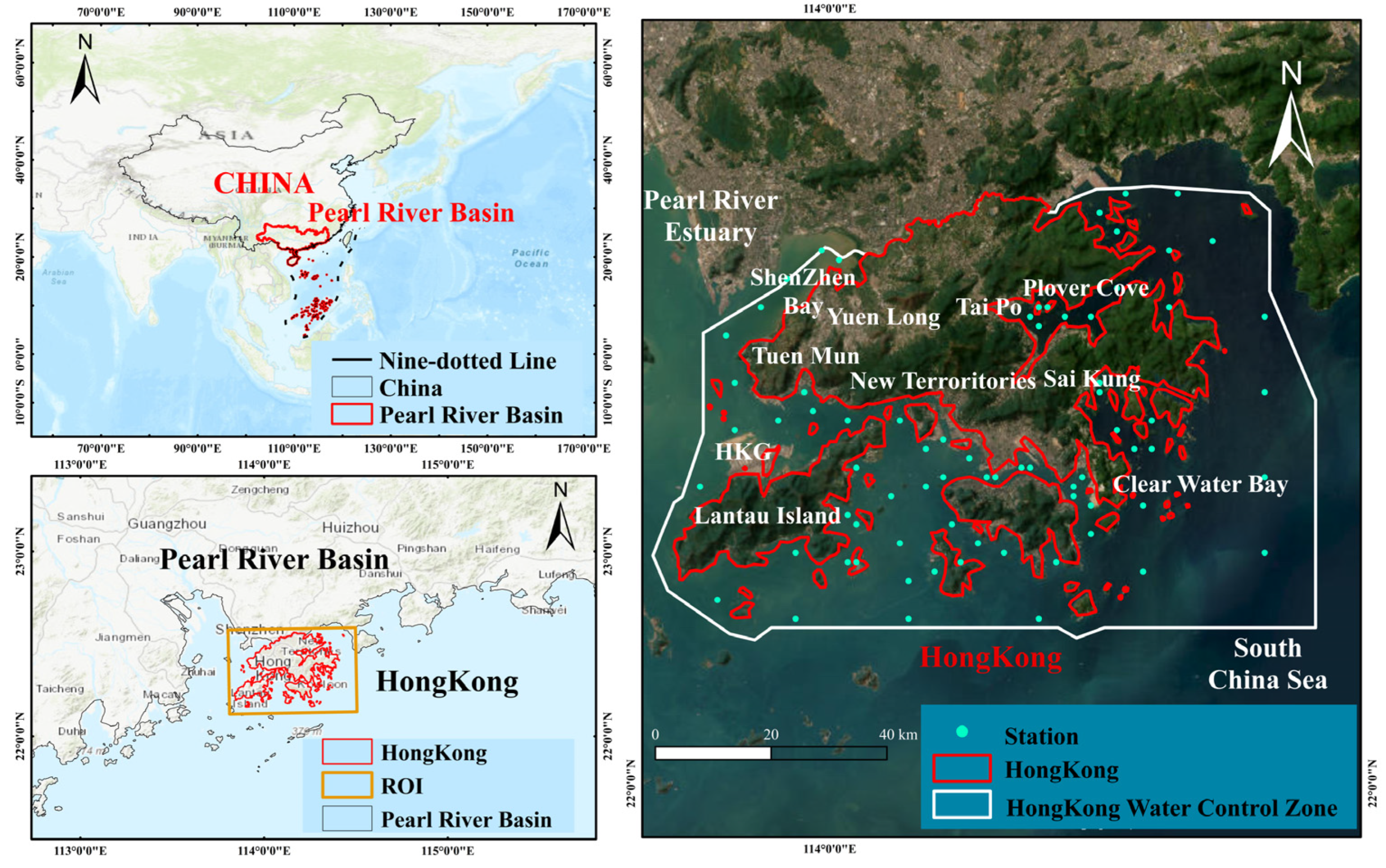
The research workflow (Figure 1) involves a systematic integration of in situ measurements, remote sensing data, and hydrometeorological and locational information. The process begins with data collection and preprocessing, where raw data from diverse sources are cleaned, normalized, and aligned temporally and spatially. For each of the WQP (TN or TP), we develop two separate models: one using only remote sensing spectral data, and the other combining spectral data with hydrometeorological and locational data.
Feature selection is performed separately in the two models using XGBoost feature importance analysis to identify key predictors. The selected features are then used to develop the inversion model with XGBoost, and hyperparameter tuning is conducted using grid search to optimize the model performance. An early stopping step is incorporated to prevent overfitting during model training. Model performance is rigorously assessed with a series of metrics in Section 2.4. The value of hydrometeorological and locational covariates is further tested with bootstrapping based uncertainty analysis. Finally, we employ the SHAP (Shapley Additive Explanations) values to investigate each predictor’s contribution to TN and TP, and to reveal potential underlying mechanisms. The workflow conducts a comprehensive comparison of models, determining the best input and model configurations, and mapping spatiotemporal changes in nutrient concentrations.

2.1. Study Area

Hong Kong, a vibrant metropolis located on the southern coast of China, is uniquely positioned at the mouth of the Pearl River Delta and experiences a subtropical climate (Figure 2). The region is characterized by a distinct hydroclimate, with hot, humid summers and mild, dry winters. This seasonal variability, alongside other climatic factors such as temperature, humidity, and wind patterns, significantly influences local water conditions, including river flows, reservoir levels, and coastal water dynamics [26].
The intricate interplay between Hong Kong’s hydroclimate and water conditions is crucial for understanding fluctuations in water quality, including the concentrations of vital nutrients such as N and P. These essential elements for aquatic ecosystems can vary dramatically with changes in climate variables that affect runoff, water temperature, and stratification. Situated at the dynamic interface of land and sea, Hong Kong’s coastal waters are particularly susceptible to the impacts of seasonal hydroclimate shifts.
Increased rainfall during the summer monsoon season can lead to elevated nutrient levels through enhanced terrestrial runoff, while the drier winter conditions may result in lower nutrient influxes. Recognizing these seasonal trends is vital for predicting and managing water quality changes over time.

2.2. Data Sources and Processing

The training data sources are detailed in Table 1. The in situ coastal water quality data are provided by the Hong Kong Environmental Protection Department (HKEPD). Remote sensing data (Aqua Moderate Resolution Imaging Spectroradiometer, MODIS) is obtained through Google Earth Engine (GEE) and preprocessed on the Google Colab. Additionally, the hydro-meteorological data are sourced from the ERA5 Daily Aggregates collection on GEE.
While both in situ data and MODIS satellite remote sensing data cover the period from 2020 to 2022, the ERA5 dataset used in this study only extends up to 9 July 2020 (Table 1). Therefore, we standardized the timeframe of all datasets to ensure consistency and reliability in the following analyses.

2.2.1. In Situ Data

The HKEPD has been tracking the health of its waters since 1986, using a robust monitoring network with 76 strategically placed stations in open waters. These monitoring stations provide monthly water quality measurements from 1986 to 2022. Table 2 provides basic statistics of eight WQPs during 2002–2020. The parameters include (i) physical and aggregate properties (SS, Turbidity, Transparency); (ii) aggregate organic constituents (Chl-a); (iii) nutrients and inorganic constituents (TP, TN, NH3-N); and (iv) biological and microbiological examination (DO). This study focuses on the inversion of TP and TN.

2.2.2. Remote Sensing Data

Our study uses the MYDOCGA Version 6 Level 2 Gridded Lite (L2G-lite) Ocean Reflectance product (2002–2023) derived from MODIS. This product offers estimates of surface spectral reflectance data spanning MODIS bands 8 through 16. Released daily, MYDOCGA.006 L2G-lite provides global coverage with a spatial resolution of 1 km. The data has been corrected for atmospheric conditions such as gasses, aerosols, and Rayleigh scattering and has been extensively validated for its applicability beyond ocean reflectance.
To filter the best quality images, we define a masking function that employs bitwise operations on quality control bands (QC_b8_15_1km and QC_b16_15_1km) to filter out pixels potentially affected by atmospheric conditions, thus retaining the ‘best available pixel’ from each MODIS image. The remote sensing data processing is performed with Google Colab.

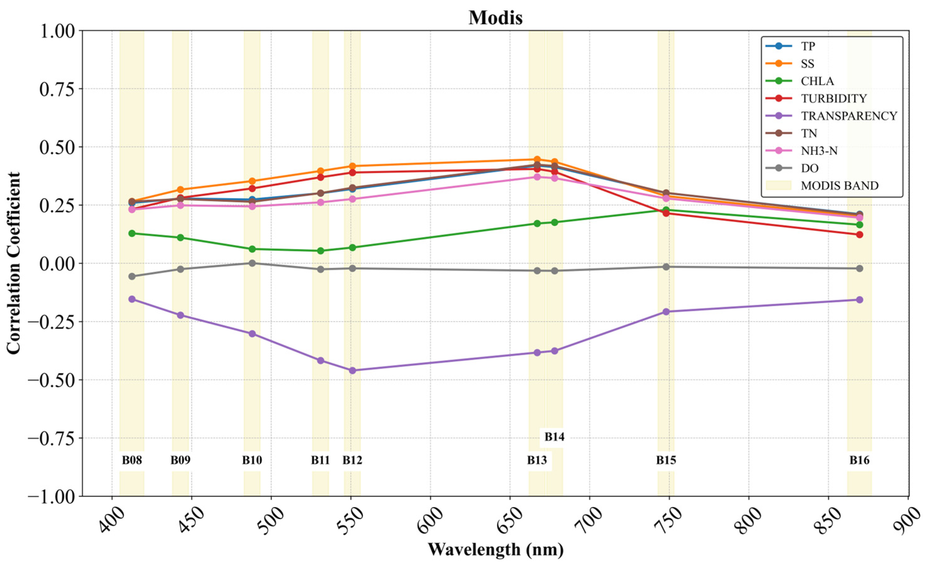
2.2.3. Key Optical Bands

From Table 3, we identify SS as the key optically sensitive substance that shows the highest correlation coefficients with TN and TP (both exceeding 0.6). Figure 3 compares correlation coefficients between WQPs and spectral bands from MODIS. SS exhibits moderate and positive correlations in MODIS bands, particularly in B12 to B15 (550–750 nm). The wavelength ranges are roughly consistent with the bands selected by the inversion models in previous studies. For instance, Li et al. [27] identified a wavelength range from 555 to 830 nm for a TN model and Gao et al. [28] identified a wavelength range from 475 to 830nm for a TP model.
According to Figure 3 and previous studies, MODIS bands B12–B15 are selected for further analysis. The correlation coefficients between each band combination and TP/TN are calculated using an enumeration method. The results, shown in Table 4, identify the band combinations with higher correlation coefficients, effectively screening out the most relevant combinations for accurate estimation of TP and TN.

2.2.4. Hydrometeorological Data

The ERA5 dataset (1979–2020) obtained from GEE in this paper provides a comprehensive set of hydrometeorological variables (Table 5), categorized into temperature, humidity, precipitation, pressure, and wind components. This dataset provides a detailed representation of atmospheric conditions, aiding in the understanding of environmental dynamics and their potential impacts on water quality. We selected the following variables to drive TN and TP inversion models: T2m_Mean (daily average air temperature measured at a height of 2 m above ground level); Precip_Total (total daily precipitation); P_Surf (daily average pressure at the Earth’s surface); U10m_Wind (daily average wind speed in the east–west direction at a height of 10 m); V10m_Wind (daily average wind speed in the north–south direction at the same height).

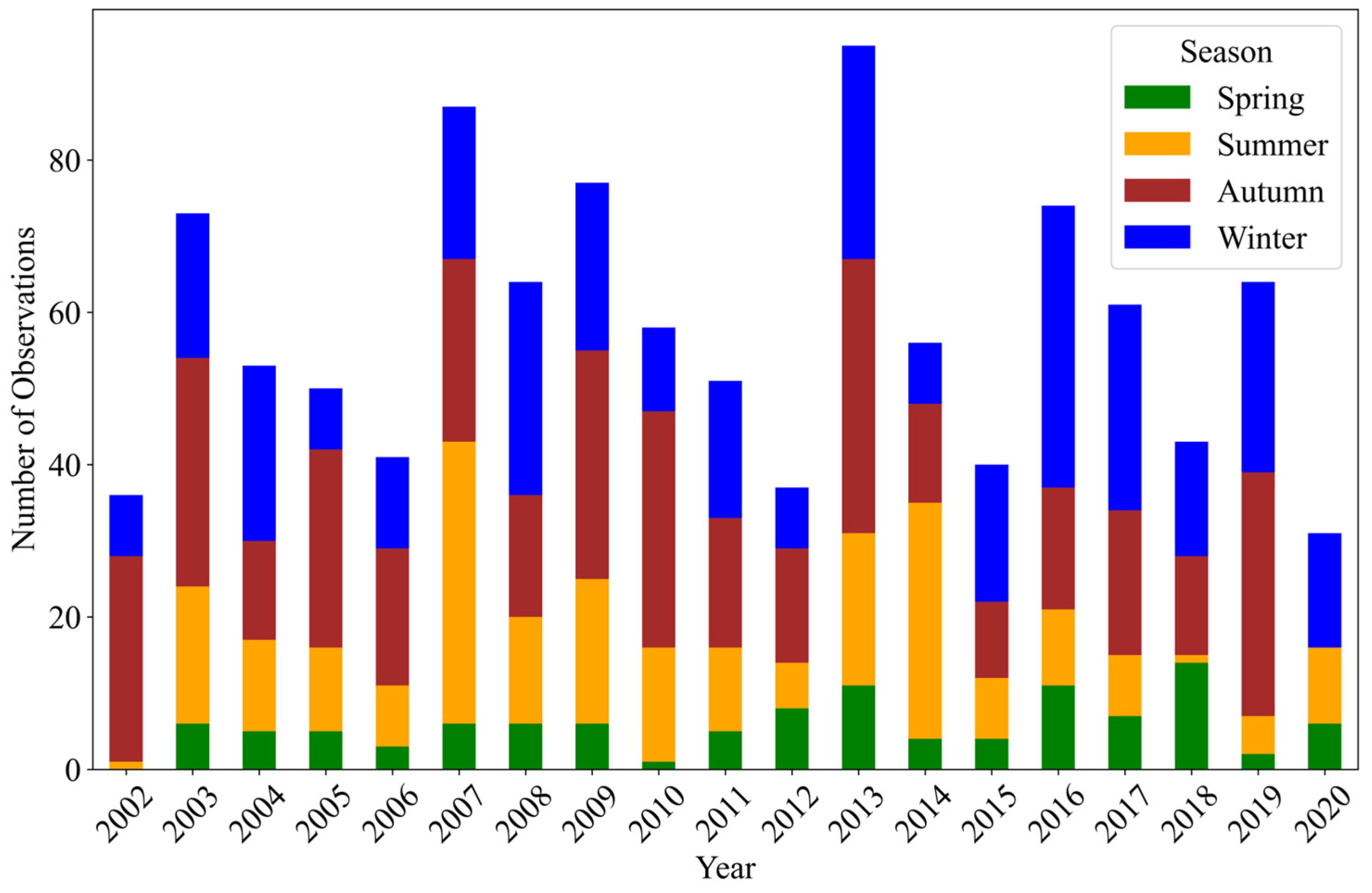
2.2.5. Match-Up Analysis

We matched the different sources of data from 2002 to 2020 and identified 1091 valid samples with complete data availability. The temporal distribution of valid samples is shown in Figure 4. The valid samples showed higher frequencies in autumn and winter, and lower frequencies in spring and summer. For reference, December to February is winter, March to May is spring, June to August is summer, and September to November is autumn.
Figure 5 presents the statistical distribution of matched data pairs. The data spans a range of 0.01 to 1 mg/L for TP and 0.07 to 11.44 mg/L for TN. The dataset exhibits skewed distributions, with a significant proportion of low concentration values and a smaller proportion of high concentration values.

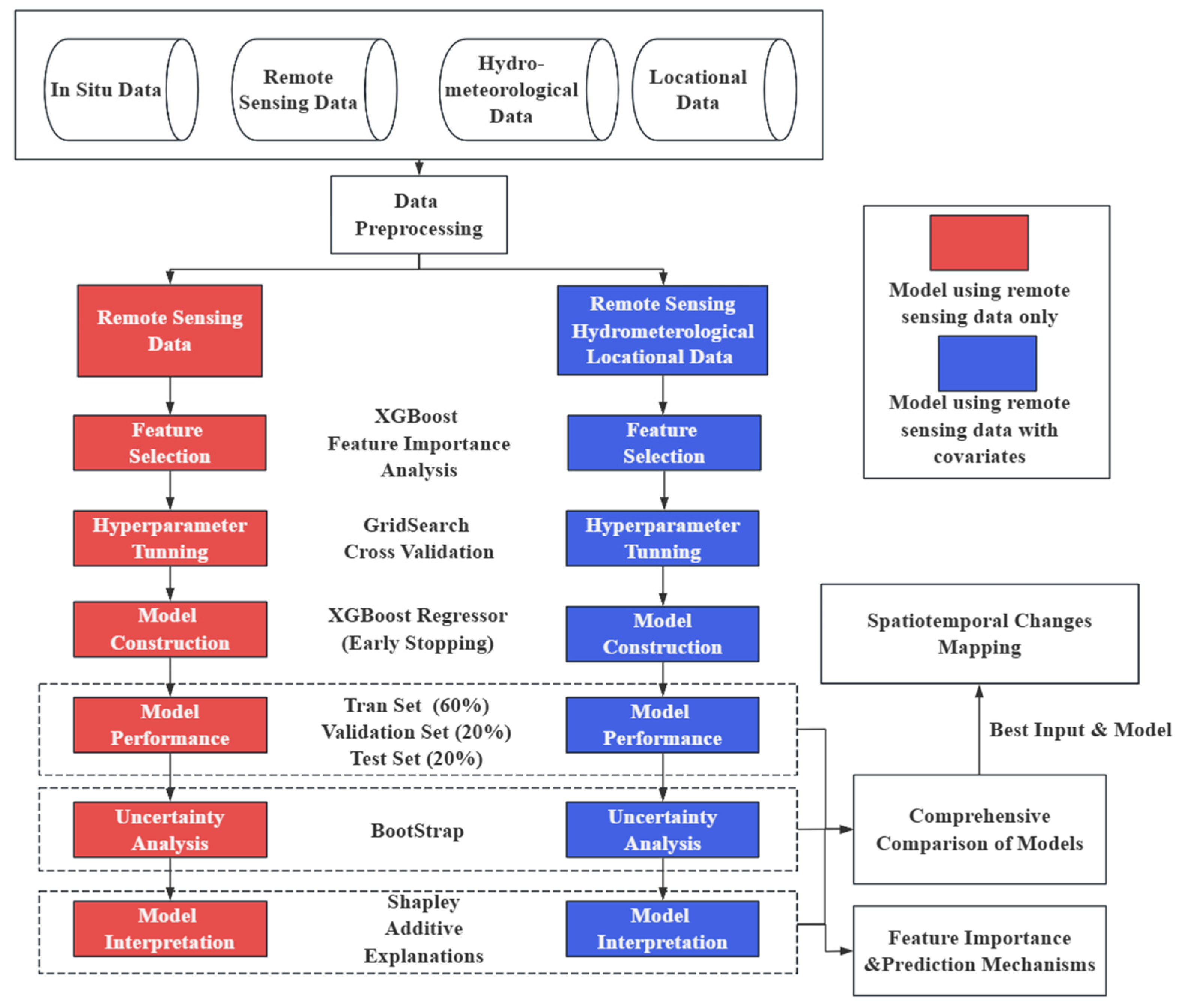
2.3. Model Development

2.3.1. Feature Selection

We implement a feature selection methodology grounded in feature importance and cross-validation to enhance model performance [29]. This method employs an XGBoost model to compute each feature’s importance score. Features are ranked in descending order based on their importance scores, which are calculated as the average of the importance scores of the ten-fold cross-validation results. Starting with the most important feature, features were incrementally added to the inversion model until the model reaches best performance, as measured by the average R2 score of cross-validation. The feature set corresponding to this optimal model was subsequently selected.

2.3.2. Hyperparameter Tuning

We implemented a hyperparameter tuning strategy using grid search with ten-fold cross-validation [30]. The feature set is standardized into the range [0, 1] to ensure each feature contributed equally to the model’s performance. The tuning process involves setting up a comprehensive parameter grid, including various values for key hyperparameters: learning rate (0.01, 0.02, 0.05, 0.1, 0.2), maximum tree depth (3, 4, 5, 6, 7, 8), subsample ratio (0.5, 0.6, 0.7, 0.8, 0.9), and the lambda regularization term (0.1, 1, 10, 50, 100). We systematically evaluated each combination of these hyperparameters and kept the combination with the best model performance.

2.3.3. Machine Learning Model

We employed XGBoost, a ML algorithm under the gradient boosting framework, to build TN and TP inversion models. XGBoost builds an ensemble of decision trees sequentially, and each tree corrects the errors of the previous ones [31]. It includes advanced features such as parallel processing, tree pruning, and missing value handling. XGBoost supports customized cost functions with L1 and L2 regularization to prevent overfitting.
In this study, early stopping was used to halt training if performance on a validation set did not improve for a specified number of iterations [32]. This ensured that the model retained the parameters from the iteration with the best validation performance, rather than potentially overfitting to the training data. The generalization capacity and robustness of XGBoost make it a popular choice in data science and machine learning studies.

2.4. Model Evaluation

2.4.1. Data Separation

We randomly separated the 1091 valid samples into training, validation, and testing sets with ratios of 0.6:0.2:0.2. The training data was used for identifying the XGBoost parameters, while the validation data was used to track the performance of XGBoost. The model training was halted when its performance did not improve in the validation set. Finally, the trained XGBoost model was tested with the testing data, and its performance indicated the model’s capability for generalizing to unseen data.

2.4.2. Algorithm Accuracy Evaluation

This study assesses the algorithm’s performance using four metrics: coefficient of determination (R2), root mean squared error (RMSE), mean relative error (MRE) and Bias.
R 2 = 1 i = 1 n y ^ i y ¯ 2 i = 1 n y i y ¯ 2
R M S E =   1 n i = 1 n ( y i y ^ i ) 2
B I A S = 1 n i = 1 n ( y i y ^ i )
M R E = 1 n i = 1 n ( y i y ^ i ) y i 100 %
where y i represents the observed value, y i ^ the predicted value, y ¯ the mean value of the observed data and n the number of match-up data pairs.

2.5. Uncertainty Analysis

Bootstrap [33] is a powerful statistical method for estimating the distribution of a statistic by resampling with replacement from the original dataset [34]. It is particularly useful for uncertainty analysis as it allows for the estimation of confidence intervals and variability measures without the need for strong parametric assumptions [35]. Additionally, the bootstrap method helps identify model robustness by providing insights into performance across different data subsets [36].
We applied the bootstrap method to analyze uncertainty in model predictions. We generated several bootstrap samples from the original dataset, with each sample created by randomly selecting data points with replacement [37]. The model was then trained on each of these bootstrapping samples, and predictions were made on the test set. We repeated this process for 1000 iterations. The predictions from all bootstrap samples were aggregated to provide a distribution of predicted values for each test set data point. We calculated the mean and standard deviation of these predictions to estimate central tendency and variability, respectively. The 95% confidence intervals were constructed using the standard deviation (mean ± 1.96 × standard deviation), allowing the assessment of model stability and reliability across different data subsets.

2.6. SHAP Model Interpretation

The complex nature of ML models often leads to a loss of interpretability, which can be a significant challenge. While some models (e.g., decision trees and support vector regression) offer inherent interpretability, this is often limited in scope [38]. Tree-based ensemble methods like gradient boosting and random forest regression can provide feature importance analysis, but these approaches tend to focus on global-level interpretations and can be difficult to compare across different models [39].
To address these limitations, we employ the SHAP framework, a model-agnostic approach that leverages Shapley values from cooperative game theory to quantify the unique contribution of each input feature to the model’s predictions [40]. SHAP can be used for both local (individual-level) and global (dataset-level) interpretations, providing a more comprehensive understanding of the underlying relationships. Specifically, SHAP fairly distributes the model’s predictions among the input variables, revealing the marginal impact of each feature on the output for both individual instances and the overall dataset. This approach allows us to gain insights into how each feature influences the predictions, enhancing the interpretability and transparency of the TN and TP inversion models.

2.7. Spatial-Temporal Distribution Analysis

We established a fishing net grid (cell size: 1 km × 1 km) over the study region to serve as the foundation for our spatial analysis. Each grids’ centroid coordinates were extracted to represent the central points for subsequent data extraction. Satellite data and hydrometeorological data were then obtained for each centroid through GEE. The optimal ML inversion models were then employed to estimate TN and TP concentrations at each grid point.
After predicting the annual concentrations of TN and TP from 2002 to 2020 at each grid point, we employed the Inverse Distance Weighted (IDW) interpolation technique to interpolate the scattered inversion model estimates into all grids [41]. We generated a comprehensive spatial distribution map depicting the average TN and TP concentrations from 2003 to 2019. To further understand the relationship between remote sensing spectral factors and TN/TP concentrations, we plotted the distributions of SHAP values for key predictors during the years 2010, 2015, and 2019. The SHAP value maps provided helpful information on the importing, transportation, and transformation of TN and TP over space and time.

3. Results

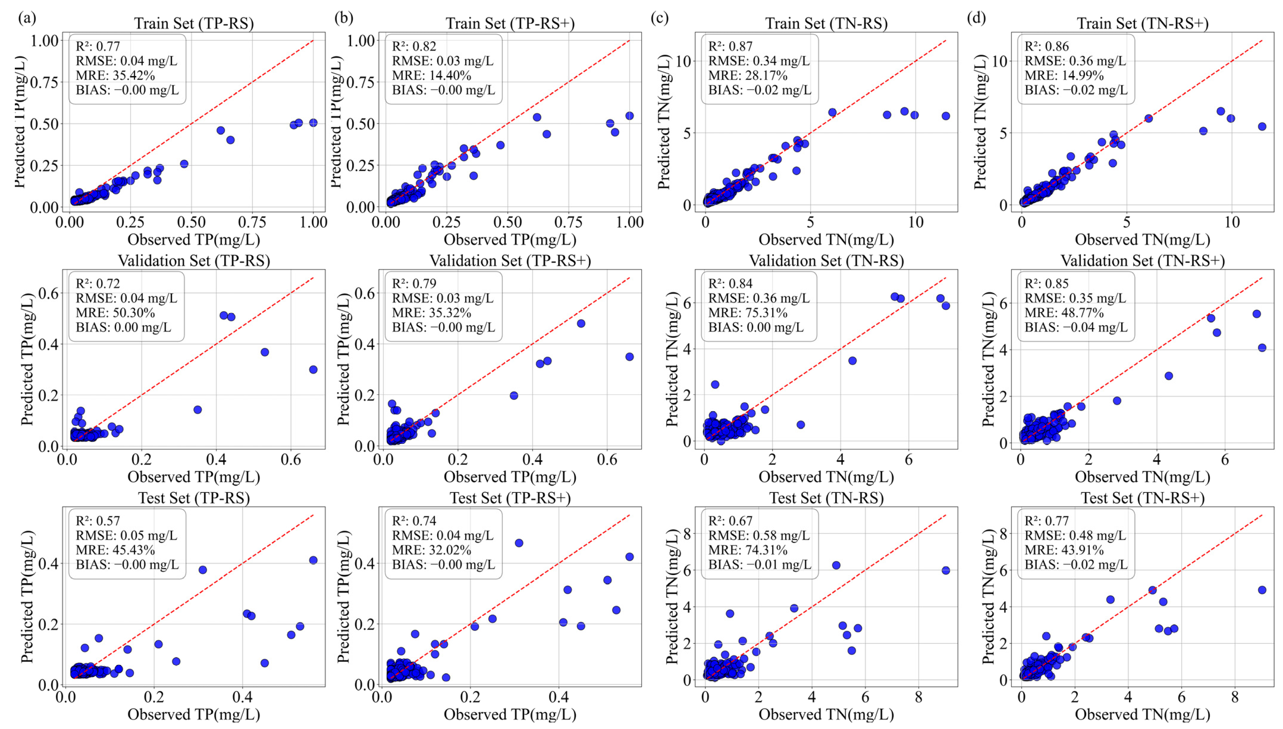
3.1. Model Performance

We develop four ML inversion models: (i) TN inversion model with only remote sensing spectral data (TN-RS), (ii) TN inversion model with remote sensing, hydrometeorological, and locational data (TN-RS+), (iii) TP inversion model with only remote sensing data (TP-RS), (iv) TP inversion model with remote sensing, hydrometeorological, and locational data (TP-RS+). The values of R2, RMSE, BIAS, and MRE for each of the models training, validation, and testing sets are shown in Figure 6.
The models with only spectral information (TN-RS and TP-RS) show decent performances during the training and validation steps (R2 exceeding 0.7), but significantly underperform with the testing set (R2 0.57 for the TP-RS model and 0.67 for the TN-RS model). This suggests a significant level of overfitting, though early stopping is employed with the validation dataset to avoid overfitting. Incorporating hydrometeorological and locational variables in the inversion model (TN-RS+ and TP-RS+) clearly improves the model’s ability to avoid overfitting. These enhanced models show similar performance to spectral-only models (TN-RS and TP-RS) during the training and validation steps, but their performance decreases only marginally with the testing set. The results thus demonstrate the generalizability of the relationship between TN and TP concentrations and hydrometeorological and locational variables.

3.2. Uncertainty Analysis

We estimate the model prediction uncertainty using the testing set by calculating the 95% confidence intervals from the bootstrapping method. We count the number of target testing samples falling within these intervals and use the Cover Ratio (CR) to quantify the performance of the confidence intervals (Figure 7). An inversion model with a high CR value suggests a better capability in capturing the observed value within its confidence interval [42]. Additionally, we quantify the uncertainty of the results by calculating the Relative Confidence Interval (CI) Width. The Relative CI Width is computed as the average width of the confidence intervals divided by the range of the predictions, expressed as a percentage. A smaller Relative CI Width indicates lower uncertainty.
For the two TP inversion models, TP-RS+ shows a much higher predictive capability with estimations closer to the observed values. Importantly, for the few testing samples with high TP concentrations, TP-RS’s confidence intervals are significantly expanded, reflecting an increase in uncertainty (Figure 7a). In contrast, the incorporation of hydrometeorological and locational variables in TP-RS+ leads to significantly smaller confidence intervals, closer to the observed TP concentrations (Figure 7b). The TP-RS+ model yields a much larger CR value (30.14%) than TP-RS (12.33%) with lower uncertainty (8.82% Relative CI Width as compared to 20.53% for TP-RS). Similarly, TN-RS+ yields a CR value of 23.74% with 12.09% Relative CI Width, as compared to 13.70% CR and 18.43% Relative CI Width for TN-RS. The results suggest that the inclusion of hydrometeorological and locational variables significantly improves the reliability of inversion models while reducing their uncertainty.

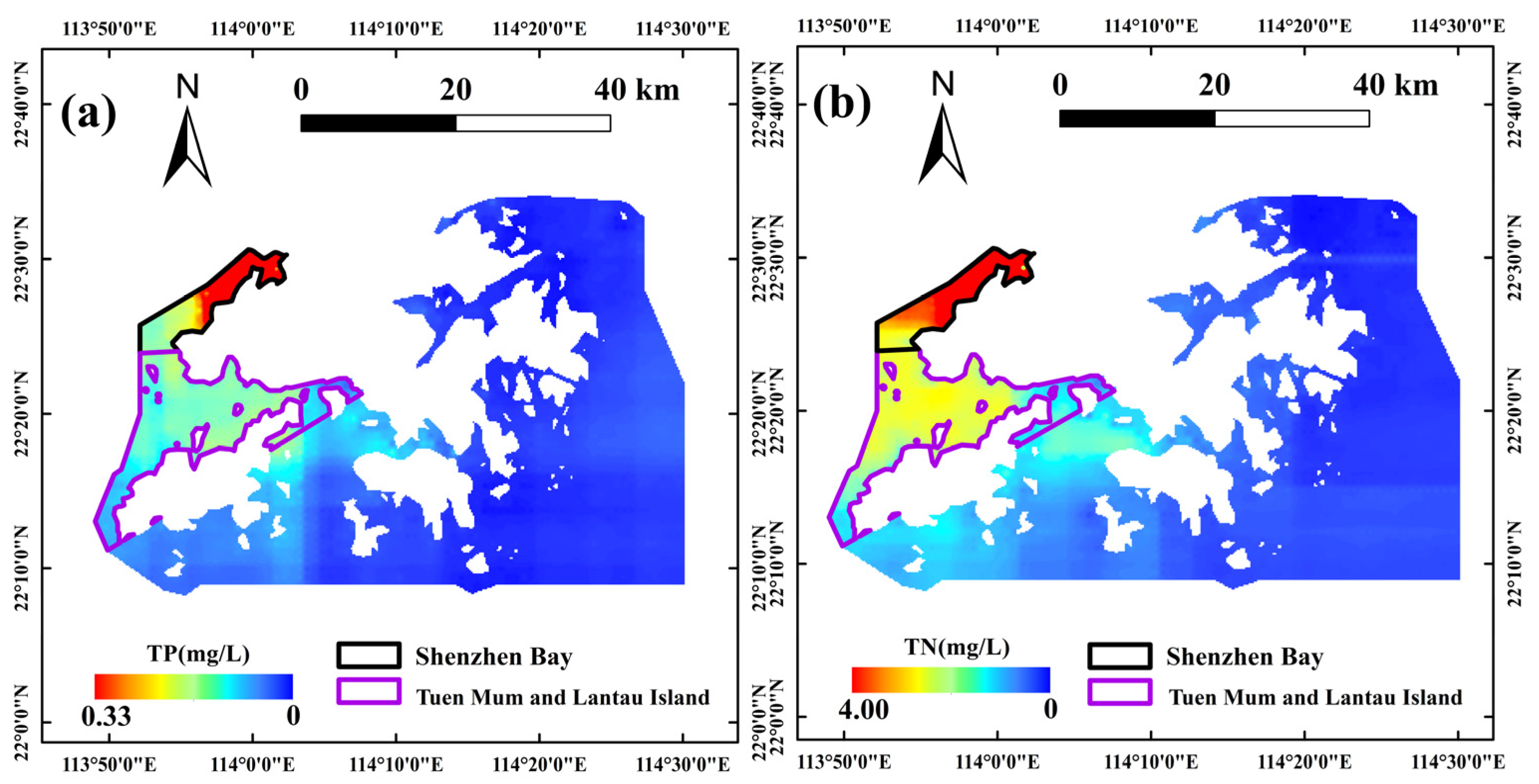
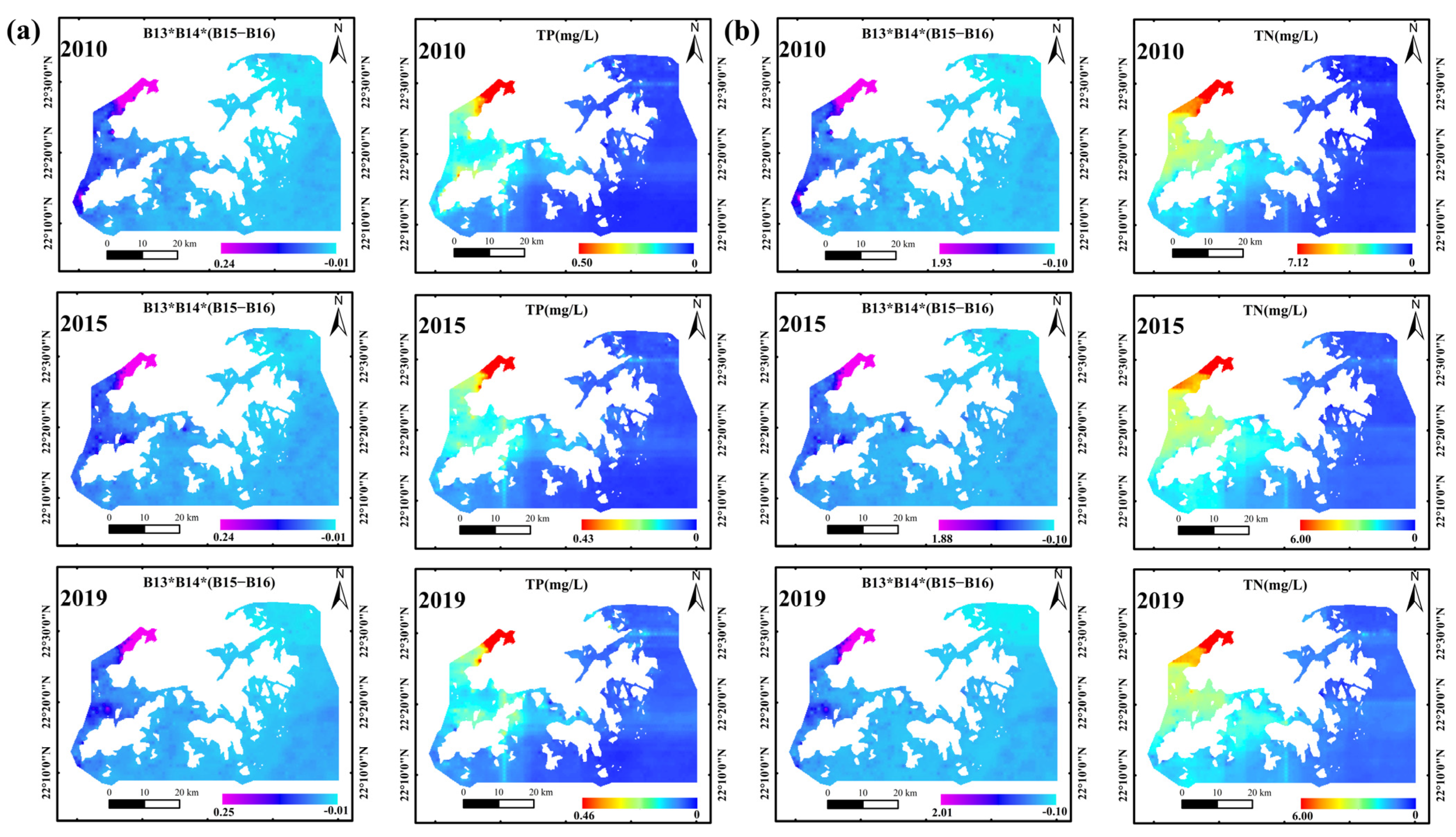
3.3. Spatial Distribution

We then estimate the TN and TP concentrations for the Hong Kong coastal region during 2003 to 2019 using the TN-RS+ and TP-RS+ models, respectively. The average TN and TP concentrations during the study period are shown in Figure 8. The highest average TP concentration reaches 0.33 mg/L, and the highest average TN concentration reaches 4.00 mg/L. Both maximum values are identified in the northwestern part of the study region. This high-concentration zone is particularly prominent near the coastal regions adjacent to the city of Shenzhen (known as Deep Bay or Shenzhen Bay).
The central and southwestern parts of the region, including Tuen Mun and parts of Lantau Island, exhibit moderate levels of nutrient pollution. The TP concentrations within this part range from 0.1 to 0.2 mg/L, and the TN concentrations range from 1.0 to 2.0 mg/L, as represented by the yellow to green shading on the maps. The eastern and southeastern parts of the region, including Sai Kung and Clear Water Bay, exhibit the lowest concentrations for both TP and TN, with values approaching 0 mg/L (the blue-shaded area in Figure 8).
While the distribution patterns for TP and TN are similar, the gradient of concentration changes is more pronounced for TN. The difference in concentration gradients suggests a difference in the transportation and transformation processes of TN and TP [43]. Specifically, nitrogen compounds in aquatic systems undergo significant spatial and temporal variations due to biological processes such as nitrification and denitrification. These processes, influenced by temperature, oxygen availability, and microbial activity, create sharp TN gradients, particularly in areas with variable oxygen levels and high microbial activity. In contrast, TP, which includes both dissolved and particulate forms, is primarily influenced by physical processes such as adsorption, sedimentation, and resuspension. These processes are generally more stable and less influenced by rapid biological transformations.

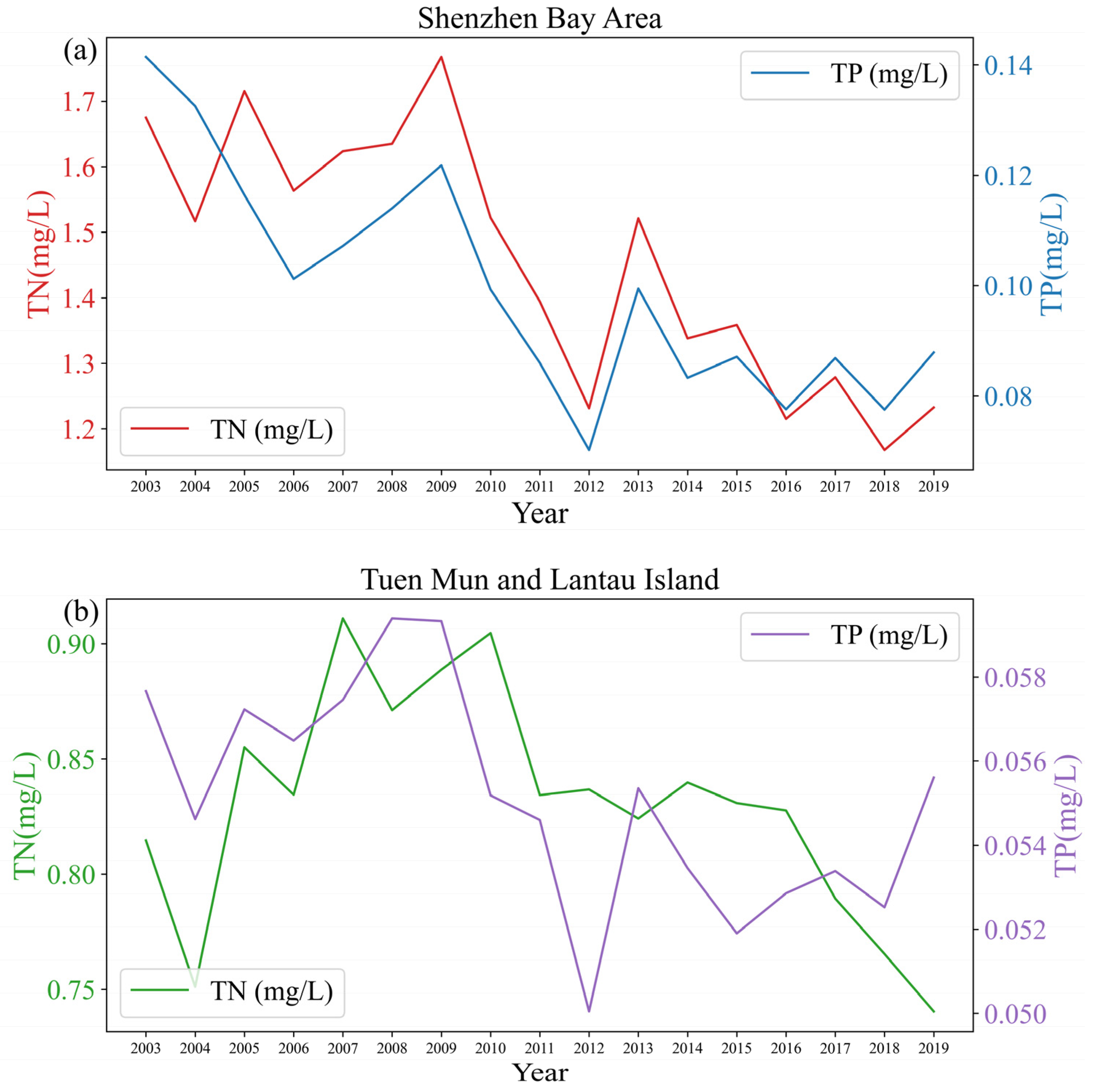
3.4. Interannual Trends

As can be seen from Figure 9a, from 2003 to 2019, the average estimated TN and TP concentrations in the Shenzhen Bay area show overall decreasing interannual trends. The average TN concentration ranges from 1.2 mg/L to 1.73 mg/L with peaks identified in 2003, 2005 and 2009. The average TP concentration ranges from 0.07 to 0.14 mg/L with two significant low points in 2012 and 2019. The average estimated TN and TP concentration trends in Tuen Mun and Lantau Island in Figure 9b show slightly different patterns. The average TN peaks in 2007 at 0.91 mg/L, then decreases linearly with fluctuation to 0.75 mg/L by 2019. In contrast, the average TP concentration does not show significant temporal variation, remaining between 0.05 mg/L to 0.058 mg/L.
Notably, TN and TP concentrations in the Shenzhen Bay Area, as well as TP concentration in Tuen Mun and Lantau Island, experienced a sharp decline after 2009, followed by an increase in 2012. This pattern may be closely linked to the 2008 global financial crisis, which resulted in a substantial reduction in trade and industrial activities in Hong Kong and Shenzhen [44], thereby reducing nutrient loadings to Hong Kong’s coastal waters. As economic activities gradually recovered, especially after the Central Government’s support for Hong Kong’s financial development under the 12th Five-Year Plan in 2011 [45], a slight rebound in nutrient levels was observed by 2012. This recovery likely reflects the recovered industrial outputs, contributing to the increase in TN and TP concentrations.

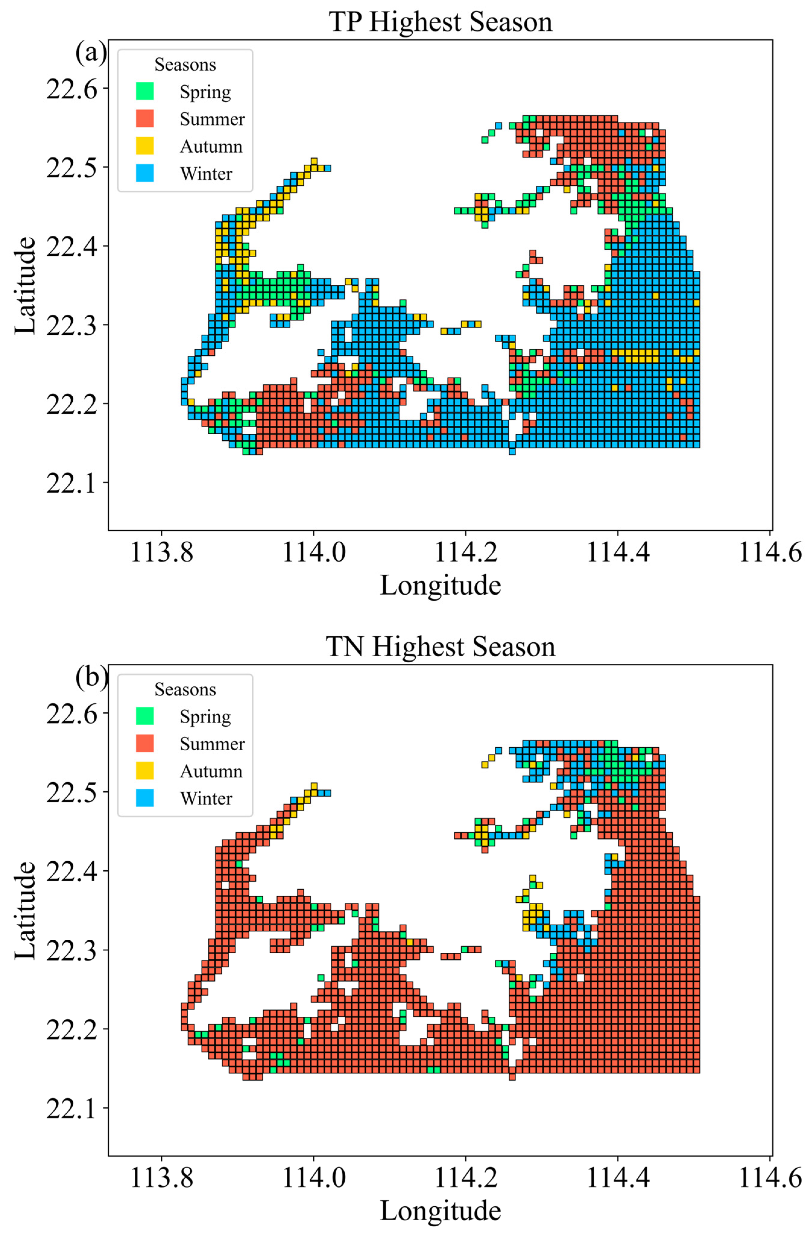
3.5. Seasonal Pattern

TP and TN distributions across the Hong Kong coastal region show significant seasonal variations, with the high-concentration season differing across various regions (Figure 10).
For TP concentration, the winter-peaking region is mostly in the eastern and southeastern coastal areas, including Sai Kung and Clear Water Bay, where TP concentrations are highest during winter. The summer-peaking regions appear in the central New Territories and extend toward Lantau Island; spring-peaking regions are scattered across the northwest near Shenzhen Bay and central regions; and autumn-peaking regions are mostly located in Shenzhen Bay (Figure 10a). In regions with high average TP concentrations, the highest TP values occur during autumn, likely due to terrestrial inputs such as leaves and crop residuals [46,47].
As for TN in Figure 10b, most regions are summer-peaking, particularly around the New Territories, including Yuen Long and Tuen Mun, extending towards southern locations such as Lantau Island and areas near Hong Kong International Airport. Winter-peaking regions concentrate in the northeastern parts of the New Territories, especially near Tai Po and Plover Cove; spring-peaking regions are mostly scattered, with notable concentrations near the southern coast of Lantau Island and some central locations. Autumn-peaking regions mostly appear in estuaries such as Shenzhen Bay. The appearance of autumn-peaking regions in Shenzhen Bay River mouth echo findings on TP temporal distribution in Figure 10a, that terrestrial inputs such as leaves and crop residuals in autumn lead to the increased nutrient concentration. However, unlike the pattern identified in TP concentration, the TN concentration further downstream of the river mouth quickly shifts to summer-peaking in Shenzhen Bay. This may be caused by the increased microorganism activity during summer, which decomposes organic matter and releases N in Shenzhen Bay [48,49].

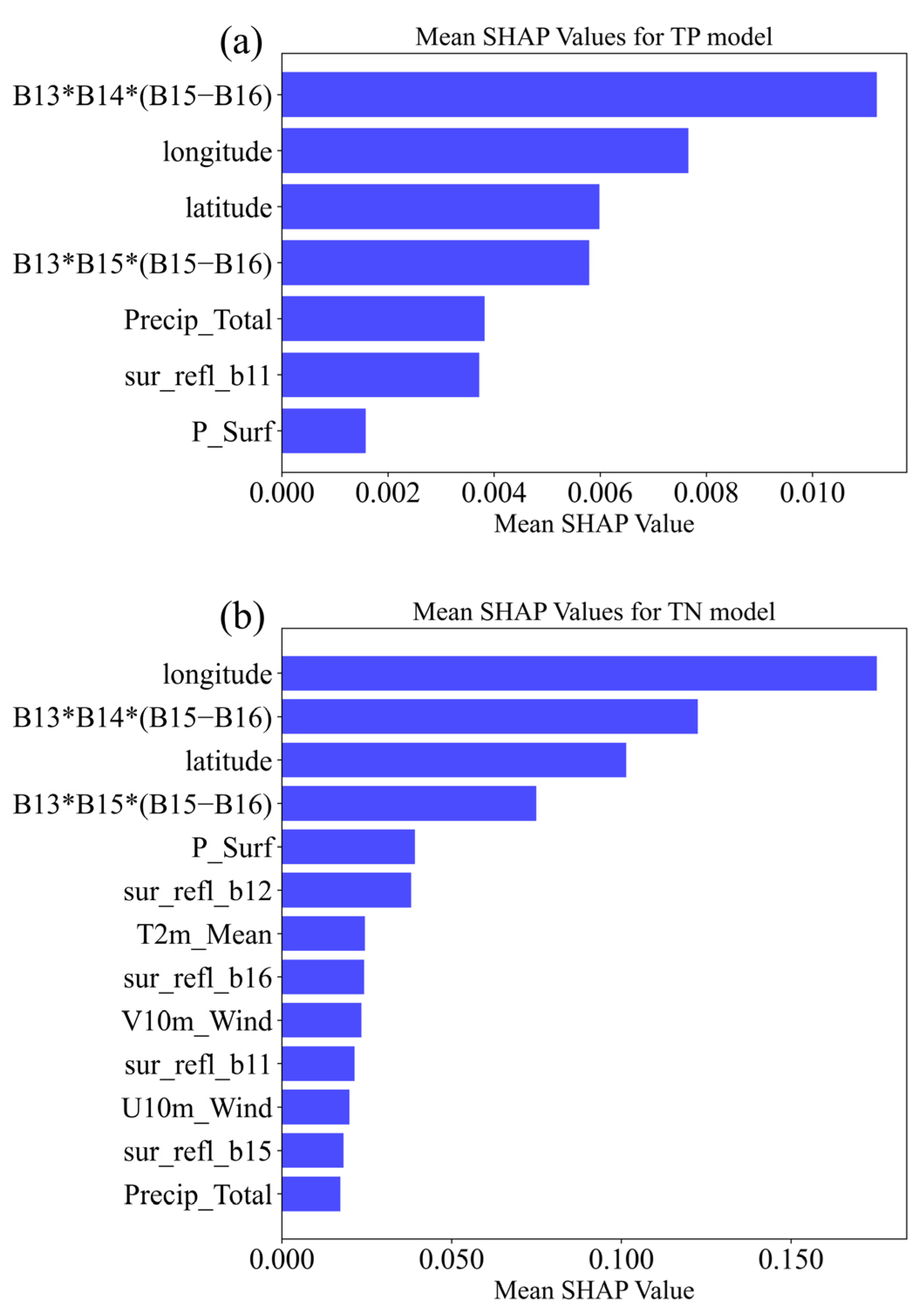
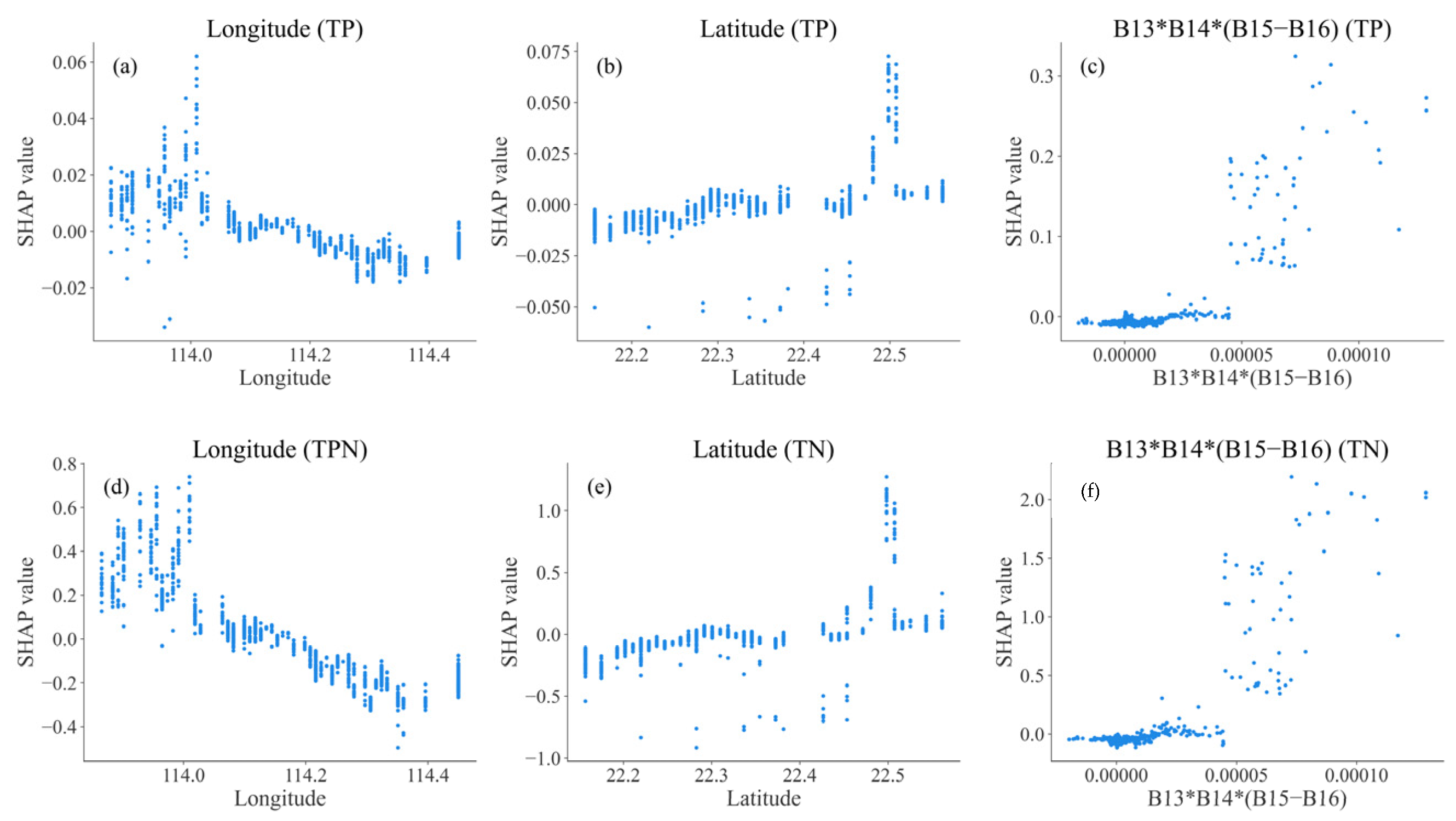
3.6. Model Interpretation

The SHAP value analysis of the TP-RS+ model provides valuable insights into the relative importance of the contributing features. As can be seen in Figure 11a, the spectral band combination B13*B14*(B15–B16) emerges as the most influential factor, underscoring the critical role of MODIS spectral information in capturing the dynamics of TP concentration in water bodies.
Interestingly, locational variables such as longitude and latitude are critical predictors of TP concentration, highlighting the consistent spatial pattern of TP concentrations in Hong Kong’s coastal regions. More specifically, Shenzhen Bay, which receives terrestrial nutrient inputs, has the highest TP concentration. This consistent spatial gradient of TP concentration between Shenzhen Bay and the rest of the study area helps in developing robust and contextually aware TP inversion predictions. Furthermore, the TP-RS+ model incorporates covariates such as total precipitation and surface pressure which contribute incrementally to the overall predictive power. These factors capture the influence of hydrological and atmospheric conditions on the complex dynamics of phosphorus in aquatic systems [50,51], underscoring the need for a multi-faceted approach to accurately model TP concentrations.
Similarly, the SHAP value analysis for the TN-RS+ model, as shown in Figure 11b, reveals that longitude is the most significant feature, emphasizing the importance of geographic location. Spectral band combinations, specifically B13*B14*(B15–B16) and B13*B15*(B15–B16), are also crucial for detecting TN concentrations. Additionally, covariates such as surface pressure, temperature, and wind components (e.g., U10m_Wind, V10m_Wind) contribute to the model, providing additional hydrological and meteorological information that refines the predictions.
SHAP dependency plots in Figure 12 provide critical insights into the influencing factors of TP and TN concentrations. Longitude exhibits a consistent negative relationship with its SHAP value for both TP and TN models, indicating that areas located further east tend to have lower nutrient concentrations. In contrast, latitude shows a positive correlation with its SHAP values for both TP and TN models, suggesting that areas located in the north have higher nutrient concentrations. The impacts of longitude and latitude indicate the importance of the northwestern edge, where Shenzhen Bay is located.
Notably, the spectral band combination B13*B14*(B15–B16) emerges as a robust predictor for both TP and TN, showing positive correlations with their SHAP values. We observe an abrupt change in this spectral band’s SHAP value at around 0.00005, above which the SHAP value significantly increases. This abrupt change may be caused by a high SS concentration, as the band combination B13*B14*(B15–B16) is sensitive to SS changes.
The above assumption is partially supported by the spatial distribution of B13*B14*(B15–B16)’s SHAP values in Figure 13. The SHAP values of B13*B14*(B15–B16) are high in Shenzhen Bay, where TN and TP concentrations are also highest (Figure 13). The temporal stability of the spectral band combination’s predictive power is evident from the consistent patterns observed in the maps over the three time periods. Despite potential changes in environmental conditions and anthropogenic influences, the spectral band combination B13*B14*(B15–B16) remains a reliable indicator of nutrient concentrations, especially in Shenzhen Bay. This stability is crucial for long-term monitoring and management of water quality, providing a dependable tool for environmental assessment.

4. Discussion

4.1. The Problem of Overfitting

Several water quality inversion studies have been conducted for Hong Kong’s coastal regions. These studies, which estimate TN, TP, total SS (TSS), and Chl-a, rely solely on remote sensing data from Landsat or Sentinel. Models developed from such studies have an R2 over 0.85 in the training set but experience a decrease of at least 0.19 in R2 in the testing set (Table 6). The overfitting problem in existing studies is also observed in our TP-RS and TN-RS models, which use only remote sensing data inputs and experience a 0.2 decrease in R2 in the testing set for both models. However, our covariate-assisted TN-RS+ and TP-RS+ models show more consistent performance across the training, validation, and testing sets. While the training R2 of TN-RS+ and TP-RS+ are lower than the previous models with only spectral data [14], their testing R2 are significantly higher with at least a 0.1 margin.
The results in Table 6 are interesting, as optically sensitive WQPs such as TSS and Chl-a also face the overfitting problem [11,52]. Such findings suggest the risk of relying solely on remote sensing data for water quality inversion. Though TSS and Chl-a are expected to correlate linearly with spectral data, this relationship may be blurred by clouds, aerosols, and other atmospheric interferences [13,53], necessitating the inclusion of covariates such as hydrometeorological and locational variables to constrain the inversion model. Such covariates are especially important for continued long-term monitoring and recording of coastal WQPs via remote sensing approaches.

4.2. Potential Mechanism

Figure 8 and the additional data in Figure 14 and Figure 15 suggest that the spatial distribution of TP and TN concentrations are influenced by a variety of environmental factors [54]. From a spatial perspective, the northwestern regions with high average TP and TN concentrations (Shenzhen Bay and Tuen Mun Lantau Island) have lower average rainfall and temperature, but higher average surface pressure. Conversely, the eastern and southeastern regions with lower concentrations have higher rainfall and temperature, but lower surface pressure.
Heavy rainfall often leads to lower TN and TP concentrations due to dilution from increased river and surface runoff. This influx of freshwater reduces nutrient concentrations in estuarine and nearshore waters. This dilution effect, demonstrated by Cloern et al. [55], occurs as the rapid transit of water through river systems during high-flow conditions limits nutrient accumulation, thus reducing their concentrations upon discharge into coastal areas.
Regions with less rainfall often experience higher nutrient concentrations due to reduced dilution and longer water residence times in estuaries. These areas typically experience significant human and agricultural activities, which contribute to nutrient loads and subsequent accumulation. Dodds et al. [56] explained that reduced water volumes, combined with continuous anthropogenic nutrient inputs, elevate nutrient levels and increase eutrophication risk. Additionally, the geomorphology of coastlines and water circulation patterns can restrict water exchange, leading to greater nutrient accumulation during drier periods.
Temperature is also closely related to the nitrification process [23]. Warmer temperatures generally accelerate biological processes, increasing the metabolic rates of microorganisms that consume or release nutrients. This can lead to faster nutrient cycling, potentially reducing TP and TP concentrations during warmer periods. Conversely, cooler water tends to slow down consumption and assimilation, potentially leading to higher nutrient concentrations.
The impact of surface pressure on nutrient concentrations may be mediated by DO concentrations. Lower air pressure generally results in lower DO saturation levels, leading to decreased DO. Conversely, higher air pressure increases DO saturation levels [24], resulting in higher DO concentrations.
Smith et al. [57] discussed the impact of oxygen levels on both aerobic and anaerobic processes, thereby affecting nutrient availability. Elevated DO levels facilitate nitrification where ammonia (NH₄⁺) is oxidized to nitrate (NO₃⁻). Conversely, during hypoxic conditions (DO < 2 mg/L), nitrate can be converted to gaseous N2 and removed from the system through denitrification [48]. When DO levels remain consistently high, denitrification is suppressed, resulting in relatively high TN concentrations in the water. Additionally, high DO concentrations can influence the release and uptake of phosphorus by microorganisms. Under aerobic conditions, certain bacteria assimilate phosphorus and store it as polyphosphate [58]. This stored phosphorus can be subsequently removed from the water under anaerobic conditions (DO < 0.1 mg/L). Otherwise, the phosphorus remains within the microbial biomass or is released back into the water column under aerobic degradation processes. As a result, high DO concentrations under elevated surface pressure inhibit phosphorus removal, leading to relatively higher TP concentrations in the water.
Wind speed also appears to be an important predictor for the TN inversion models. As shown in Figure 15, northeasterly winds prevail in Hong Kong as a whole, with lower wind speeds in the northwest and higher wind speeds in the east and southeast. High wind speeds in these regions may increase the mixing of oxygen-rich marine surface waters with deeper waters [59], thereby promoting nitrification with increased DO concentrations. Meanwhile, the eastern and southeastern regions are characterized by high temperature and low pressure, which can maintain hypoxic conditions to support denitrification processes. As a result, the TN concentrations in these regions are relatively low. As for the northwestern regions such as Shenzhen Bay, the plume from the Pearl River is pushed westward by the coastal currents induced by northeasterly winds, the nutrient-rich waters from the Pearl River Estuary that flow towards the vicinity of the Shenzhen Bay Estuary may significantly increase nutrient concentrations in these regions [60,61,62].

4.3. Limitations and Future Directions

While the current research demonstrates the advantage of incorporating hydrometeorological and locational covariates in remote sensing inversion of TN and TP concentrations in Hong Kong’s coastal region, several critical limitations persist. A primary limitation is the underrepresentation of high-concentration samples in the training dataset, which undermines the model’s accuracy and reliability in predicting extreme nutrient values. For instance, the maximum observed values of TP and TN are 1.3 mg/L and 15.02 mg/L, respectively, and the model may significantly underestimate TP and TN concentrations when actual concentrations are over the maximum values. Additionally, the model may not adequately capture the complex, non-linear relationships and regional variabilities inherent in diverse aquatic environments, due to its limited complexity and adaptability. Overfitting to low-concentration data further constrains the model’s generalizability and robustness. Another significant limitation is that the impact of locational variables may change over time. The model developed here may not be as effective a few years later when the economic and human activities change in Shenzhen and Hong Kong. This temporal variability necessitates continuous model validation and updating to maintain its effectiveness. Last but not least, while the model has successfully reduced the impact of overfitting, it is not directly transferable to other regions without retraining. Each region’s unique environmental and anthropogenic factors require region-specific calibration to ensure accurate predictions [63].
Future research should prioritize the enhancement of the dataset for a more balanced representation of high-concentration and low-concentration samples to improve predictive accuracy across the entire concentration spectrum [64]. However, it can be difficult to obtain more high-concentration observations. Thus, to deal with skewed distributions with extreme values, techniques like Synthetic Minority Over-sampling Technique (SMOTE) or anomaly detection methods could be beneficial to balance the dataset and mitigate the bias towards low-concentration data. Employing more sophisticated machine learning techniques could significantly enhance model complexity, allowing for better handling of non-linear interactions and site-specific characteristics. Continuous validation and iterative model updating are crucial to maintaining model performance under varying environmental conditions and across different temporal and spatial scales [65].
The launch of the Plankton, Aerosol, Cloud, Ocean Ecosystem (PACE) satellite opens new avenues for enhancing water quality monitoring. With advanced instruments like the Ocean Color Instrument (OCI) and the Multi-angle Polarimeters, PACE captures high-resolution hyperspectral images from 350 to 885 nanometers at 5 nm intervals, covering a broad spectrum from UV to near-infrared [66]. This may introduce better direct relationships between remote sensing reflectance and non-optically sensitive water quality parameters such as TN and TP. Additionally, PACE will investigate the interactions between the ocean and atmosphere, examining how aero-sols, clouds, and phytoplankton influence each other [67], hence providing better reflectance data for the ocean environment. The launch of PACE may then lead to more accurate inversion models for WQPs in coastal waters.
Furthermore, anthropogenic drivers (e.g., urbanization, industrial activities, and land use changes) and hydrological variables (e.g., tidal flows and sediment interactions) can be additional covariates for the inversion models [68]. Integrating these additional variables can help to develop a more holistic and accurate model, ultimately leading to more effective and informed environmental monitoring and management strategies. These enhancements will not only refine the model’s predictive capabilities but also bolster its practical applicability in the context of dynamic and multifaceted coastal ecosystems.

5. Conclusions

This study successfully integrated remote sensing data, in situ measurements, hydrometeorological information and locational data to improve the estimation of TN and TP concentrations in Hong Kong’s coastal waters. Our approach demonstrates notable improvements in model performance, especially for the purpose of overfitting avoidance and uncertainty reduction.
Our results suggest TN and TP concentrations are highest in Shenzhen Bay, and this region’s concentrations were declining during 2009–2019. Spectral information, locational variables (longitude and latitude), and hydrometeorological variables (precipitation, temperature, surface pressure and wind speed) are proven to be dominant predictors of TN and TP concentrations. The high quality, mechanism-evidenced TN and TP inversion models developed in this study provide a valuable foundation for water quality management in Hong Kong’s coastal regions. Our study also provides a promising framework for reducing model overfitting in remote sensing inversion of nutrients in coastal water, but the developed model needs to be adapted and validated with region-specific data to ensure accuracy and reliability.

Author Contributions

Conceptualization, Z.Z., C.L. and P.Y.; Data curation, Z.Z.; Formal analysis, Z.Z., C.L. and P.Y.; Funding acquisition, P.Y. and Q.T.; Investigation, Z.Z., C.L. and P.Y.; Methodology, Z.Z., C.L. and P.Y.; Project administration, P.Y. and Q.T.; Software, Z.Z.; Supervision, P.Y.; Visualization, Z.Z.; Writing—original draft, Z.Z.; Writing—review and editing, P.Y., Z.X., L.Y., Q.W., G.C. and Q.T. All authors have read and agreed to the published version of the manuscript.

Funding

The work is financially supported by National Key R&D Program of China (grant number 2022YFC3202200), the Basic Science Center Project of the Natural Science Foundation of China (52388101), National Natural Science Foundation of China (grant number 52209009, 52125902), Guangdong Provincial Key Laboratory Project (grant number 2023B1212060068) and Guangdong Foundation for Program of Science and Technology Research (Grant No. 2023B1212060044).

Data Availability Statement

The measured water quality data are available from HKEPD (https://www.epd.gov.hk/epd/sc_chi/environmentinhk/water/hkwqrc/waterquality/marine.html/, accessed on 24 May 2024). The ocean reflectance product of MODIS is available on GEE (https://earthengine.google.com/, accessed on 24 May 2024). ERA5 daily aggregated data can be downloaded through GEE as well (https://earthengine.google.com/, accessed on 24 May 2024).

Acknowledgments

We thank the developers for their tools and the respective agencies that provided the data.

Conflicts of Interest

The authors declare no conflicts of interest.

References

  1. Creel, L. Ripple Effects: Population and Coastal Regions; Population Reference Bureau: Washington, DC, USA, 2003. [Google Scholar]
  2. Clark, J.R. Coastal Zone Management Handbook; CRC Press/Lewis Publishers: Boca Raton, FL, USA, 2018. [Google Scholar]
  3. Kitamori, K.; Manders, T.; Dellink, R.; Tabeau, A. OECD Environmental Outlook to 2050: The Consequences of Inaction; 92641221468; OECD: Paris, France, 2012. [Google Scholar]
  4. World Health Organization; UNICEF. Meeting the MDG Drinking Water and Sanitation Target: The Urban and Rural Challenge of the Decade; World Health Organization: Geneva, Switzerland; UNICEF: New York, NY, USA, 2006. [Google Scholar]
  5. Nixon, S. Marine Eutrophication: A Growing International Problem. Ambio 1990, 19, 101. [Google Scholar]
  6. Bartram, J.; Ballance, R. (Eds.) Water Quality Monitoring: A Practical Guide to the Design and Implementation of Freshwater Quality Studies and Monitoring Programmes; CRC Press: Boca Raton, FL, USA, 1996. [Google Scholar]
  7. Ritchie, J.C.; Zimba, P.V.; Everitt, J.H. Remote Sensing Techniques to Assess Water Quality. Photogramm. Eng. Remote Sens. 2003, 69, 695–704. [Google Scholar] [CrossRef]
  8. Mouw, C.B.; Greb, S.; Aurin, D.; DiGiacomo, P.M.; Lee, Z.; Twardowski, M.; Binding, C.; Hu, C.; Ma, R.; Moore, T.; et al. Aquatic Color Radiometry Remote Sensing of Coastal and Inland Waters: Challenges and Recommendations for Future Satellite Missions. Remote Sens. Environ. 2015, 160, 15–30. [Google Scholar] [CrossRef]
  9. Wong, M.-S.; Lee, K.-H.; Kim, Y.-J.; Nichol, J.E.; Li, Z.; Emerson, N. Modeling of Suspended Solids and Sea Surface Salinity in Hong Kong Using Aqua/MODIS Satellite Images. Korean J. Remote Sens. 2007, 23, 161–169. [Google Scholar]
  10. Hafeez, S.; Wong, M.S.; Ho, H.C.; Nazeer, M.; Nichol, J.; Abbas, S.; Tang, D.; Lee, K.H.; Pun, L. Comparison of Machine Learning Algorithms for Retrieval of Water Quality Indicators in Case-II Waters: A Case Study of Hong Kong. Remote Sens. 2019, 11, 617. [Google Scholar] [CrossRef]
  11. Liu, J.; Qiu, Z.; Feng, J.; Wong, K.P.; Tsou, J.Y.; Wang, Y.; Zhang, Y. Monitoring Total Suspended Solids and Chlorophyll-a Concentrations in Turbid Waters: A Case Study of the Pearl River Estuary and Coast Using Machine Learning. Remote Sens. 2023, 15, 5559. [Google Scholar] [CrossRef]
  12. Dong, L.; Wang, D.; Song, L.; Gong, F.; Chen, S.; Huang, J.; He, X. Monitoring Dissolved Oxygen Concentrations in the Coastal Waters of Zhejiang Using Landsat-8/9 Imagery. Remote Sens. 2024, 16, 1951. [Google Scholar] [CrossRef]
  13. Gholizadeh, M.H.; Melesse, A.M.; Reddi, L. A Comprehensive Review on Water Quality Parameters Estimation Using Remote Sensing Techniques. Sensors 2016, 16, 1298. [Google Scholar] [CrossRef]
  14. Li, H.; Zhang, G.; Zhu, Y.; Kaufmann, H.; Xu, G. Inversion and Driving Force Analysis of Nutrient Concentrations in the Ecosystem of the Shenzhen-Hong Kong Bay Area. Remote Sens. 2022, 14, 3694. [Google Scholar] [CrossRef]
  15. Song, K.; Li, L.; Tedesco, L.; Li, S.; Shi, K.; Hall, B. Remote Estimation of Nutrients for a Drinking Water Source through Adaptive Modeling. Water Resour. Manag. 2014, 28, 2563–2581. [Google Scholar] [CrossRef]
  16. Xiong, J.; Lin, C.; Ma, R.; Cao, Z. Remote Sensing Estimation of Lake Total Phosphorus Concentration Based on MODIS: A Case Study of Lake Hongze. Remote Sens. 2019, 11, 2068. [Google Scholar] [CrossRef]
  17. Wang, D.; Cui, Q.; Gong, F.; Wang, L.; He, X.; Bai, Y. Satellite Retrieval of Surface Water Nutrients in the Coastal Regions of the East China Sea. Remote Sens. 2018, 10, 1896. [Google Scholar] [CrossRef]
  18. Zheng, H.; Wu, Y.; Han, H.; Wang, J.; Liu, S.; Xu, M.; Cui, J.; Yasir, M. Utilizing Residual Networks for Remote Sensing Estimation of Total Nitrogen Concentration in Shandong Offshore Areas. Front. Mar. Sci. 2024, 11, 1336259. [Google Scholar] [CrossRef]
  19. Chang, N.-B.; Xuan, Z.; Yang, Y.J. Exploring Spatiotemporal Patterns of Phosphorus Concentrations in a Coastal Bay with MODIS Images and Machine Learning Models. Remote Sens. Environ. 2013, 134, 100–110. [Google Scholar] [CrossRef]
  20. Wang, X.; Jiang, Y.; Jiang, M.; Cao, Z.; Li, X.; Ma, R.; Xu, L.; Xiong, J. Estimation of Total Phosphorus Concentration in Lakes in the Yangtze-Huaihe Region Based on Sentinel-3/OLCI Images. Remote Sens. 2023, 15, 4487. [Google Scholar] [CrossRef]
  21. Paerl, H.W.; Huisman, J. Climate Change: A Catalyst for Global Expansion of Harmful Cyanobacterial Blooms. Environ. Microbiol. Rep. 2009, 1, 27–37. [Google Scholar] [CrossRef]
  22. Howarth, R.W.; Anderson, D.; Cloern, J.E.; Elfring, C.; Hopkinson, C.S.; Lapointe, B.; Malone, T.; Marcus, N.; McGlathery, K.; Sharpley, A.N.; et al. Nutrient Pollution of Coastal Rivers, Bays, and Seas. Issues Ecol. 2000, 7, 1–16. [Google Scholar]
  23. Delpla, I.; Jung, A.-V.; Baures, E.; Clement, M.; Thomas, O. Impacts of Climate Change on Surface Water Quality in Relation to Drinking Water Production. Environ. Int. 2009, 35, 1225–1233. [Google Scholar] [CrossRef]
  24. Boyd, C.E.; Boyd, C.E. Dissolved Oxygen and Other Gases. In Water Quality; Springer: Cham, Switzerland, 2020; pp. 135–162. [Google Scholar]
  25. Van Vliet, M.T.; Thorslund, J.; Strokal, M.; Hofstra, N.; Flörke, M.; Ehalt Macedo, H.; Nkwasa, A.; Tang, T.; Kaushal, S.S.; Kumar, R.; et al. Global River Water Quality under Climate Change and Hydroclimatic Extremes. Nat. Rev. Earth Environ. 2023, 4, 687–702. [Google Scholar] [CrossRef]
  26. Feng, T.; Xu, N. Satellite-Based Monitoring of Annual Coastal Reclamation in Shenzhen and Hong Kong since the 21st Century: A Comparative Study. J. Mar. Sci. Eng. 2021, 9, 48. [Google Scholar] [CrossRef]
  27. Li, Y.; Zhang, Y.; Shi, K.; Zhu, G.; Zhou, Y.; Zhang, Y.; Guo, Y. Monitoring Spatiotemporal Variations in Nutrients in a Large Drinking Water Reservoir and Their Relationships with Hydrological and Meteorological Conditions Based on Landsat 8 Imagery. Sci. Total Environ. 2017, 599, 1705–1717. [Google Scholar] [CrossRef]
  28. Gao, Y.; Gao, J.; Yin, H.; Liu, C.; Xia, T.; Wang, J.; Huang, Q. Remote Sensing Estimation of the Total Phosphorus Concentration in a Large Lake Using Band Combinations and Regional Multivariate Statistical Modeling Techniques. J. Environ. Manag. 2015, 151, 33–43. [Google Scholar] [CrossRef] [PubMed]
  29. Kohavi, R. A Study of Cross-Validation and Bootstrap for Accuracy Estimation and Model Selection; IJCAI: Montreal, QC, Canada, 1995; Volume 14, pp. 1137–1145. [Google Scholar]
  30. Bergstra, J.; Bengio, Y. Random Search for Hyper-Parameter Optimization. J. Mach. Learn. Res. 2012, 13, 281–305. [Google Scholar]
  31. Chen, T.; Guestrin, C. XGBoost: A scalable tree boosting system. In Proceedings of the 22nd ACM SIGKDD International Conference on Knowledge Discovery and Data Mining, San Francisco, CA, USA, 13–17 August 2016; pp. 785–794. [Google Scholar]
  32. Prechelt, L. Early Stopping|but when? In Lecture Notes in Computer Science; Springer: Berlin/Heidelberg, Germany, 1998; pp. 55–69. ISBN 978-3-642-35288-1/978-3-642-35289-8. [Google Scholar]
  33. Efron, B.; Tibshirani, R.J. An Introduction to the Bootstrap; Chapman and Hall: New York, NY, USA, 1993. [Google Scholar]
  34. Efron, B. Bootstrap methods: Another look at the jackknife. Ann. Stat. 1979, 7, 1–26. [Google Scholar] [CrossRef]
  35. Chernick, M.R. Bootstrap Methods: A Guide for Practitioners and Researchers, 2nd ed.; John Wiley & Sons, Inc.: Hoboken, NJ, USA, 2007. [Google Scholar]
  36. Mooney, C.Z.; Duval, R.D. Bootstrapping: A Nonparametric Approach to Statistical Inference, 1st ed.; SAGE Publishing: Thousand Oaks, CA, USA, 1993. [Google Scholar]
  37. Davison, A.C.; Hinkley, D.V. Bootstrap Methods and Their Application; Cambridge University Press: Cambridge, UK, 1997. [Google Scholar]
  38. Zou, H.; Hastie, T. Regularization and Variable Selection via the Elastic Net. J. R. Stat. Soc. Ser. B Stat. Methodol. 2005, 67, 301–320. [Google Scholar] [CrossRef]
  39. Breiman, L. Random Forests. Mach. Learn. 2001, 45, 5–32. [Google Scholar] [CrossRef]
  40. Shapley, L.S. 17. A value for n-person games. In Contributions to the Theory of Games (AM-28), Volume II; Princeton University Press: Princeton, NJ, USA, 2016; pp. 307–318. [Google Scholar]
  41. Lu, G.Y.; Wong, D.W. An Adaptive Inverse-Distance Weighting Spatial Interpolation Technique. Comput. Geosci. 2008, 34, 1044–1055. [Google Scholar] [CrossRef]
  42. Yang, P.; Ng, T.L. Quantifying Uncertainty in Multivariate Quantile Estimation of Hydrometeorological Extremes via Copula: A Comparison between Bootstrapping and Markov Chain Monte Carlo. Int. J. Clim. 2022, 42, 4621–4638. [Google Scholar] [CrossRef]
  43. Boynton, W.; Garber, J.; Summers, R.; Kemp, W. Inputs, Transformations, and Transport of Nitrogen and Phosphorus in Chesapeake Bay and Selected Tributaries. Estuaries 1995, 18, 285–314. [Google Scholar] [CrossRef]
  44. Kou, Y.; Liu, L.; Tian, X. The Impact of the Financial Tsunami on Hong Kong Port. Asian J. Shipp. Logist. 2011, 27, 259–278. [Google Scholar] [CrossRef]
  45. Xiaobin, Z.S.; Qionghua, L.; Ming, C.N.Y. The Rise of China and the Development of Financial Centres in Hong Kong, Beijing, Shanghai, and Shenzhen. J. Glob. Stud. 2013, 4, 32–62. [Google Scholar]
  46. Wang, Y.; Law, R.; Pak, B. A Global Model of Carbon, Nitrogen and Phosphorus Cycles for the Terrestrial Biosphere. Biogeosciences 2010, 7, 2261–2282. [Google Scholar] [CrossRef]
  47. Yan, Z.; Han, W.; Peñuelas, J.; Sardans, J.; Elser, J.J.; Du, E.; Reich, P.B.; Fang, J. Phosphorus Accumulates Faster than Nitrogen Globally in Freshwater Ecosystems under Anthropogenic Impacts. Ecol. Lett. 2016, 19, 1237–1246. [Google Scholar] [CrossRef]
  48. Herbert, R. Nitrogen Cycling in Coastal Marine Ecosystems. FEMS Microbiol. Rev. 1999, 23, 563–590. [Google Scholar] [CrossRef] [PubMed]
  49. Arrigo, K.R. Marine Microorganisms and Global Nutrient Cycles. Nature 2005, 437, 349–355. [Google Scholar] [CrossRef] [PubMed]
  50. Andersen, H.E.; Kronvang, B.; Larsen, S.E.; Hoffmann, C.C.; Jensen, T.S.; Rasmussen, E.K. Climate-Change Impacts on Hydrology and Nutrients in a Danish Lowland River Basin. Sci. Total Environ. 2006, 365, 223–237. [Google Scholar] [CrossRef]
  51. Bouraoui, F.; Grizzetti, B.; Granlund, K.; Rekolainen, S.; Bidoglio, G. Impact of Climate Change on the Water Cycle and Nutrient Losses in a Finnish Catchment. Clim. Chang. 2004, 66, 109–126. [Google Scholar] [CrossRef]
  52. Wang, X.; Cui, J.; Xu, M. A Chlorophyll-a Concentration Inversion Model Based on Backpropagation Neural Network Optimized by an Improved Metaheuristic Algorithm. Remote Sens. 2024, 16, 1503. [Google Scholar] [CrossRef]
  53. Fisher, D.C.; Oppenheimer, M. Atmospheric Nitrogen Deposition and the Chesapeake Bay Estuary. Ambio 1991, 20, 102–108. [Google Scholar]
  54. Qiu, J.; Shen, Z.; Leng, G.; Xie, H.; Hou, X.; Wei, G. Impacts of Climate Change on Watershed Systems and Potential Adaptation through BMPs in a Drinking Water Source Area. J. Hydrol. 2019, 573, 123–135. [Google Scholar] [CrossRef]
  55. Cloern, J.E.; Abreu, P.C.; Carstensen, J.; Chauvaud, L.; Elmgren, R.; Grall, J.; Greening, H.; Johansson, J.O.R.; Kahru, M.; Sherwood, E.T.; et al. Human Activities and Climate Variability Drive Fast-Paced Change across the World’s Estuarine–Coastal Ecosystems. Glob. Chang. Biol. 2016, 22, 513–529. [Google Scholar] [CrossRef] [PubMed]
  56. Dodds, W.K.; Bouska, W.W.; Eitzman, J.L.; Pilger, T.J.; Pitts, K.L.; Riley, A.J.; Schloesser, J.T.; Thornbrugh, D.J. Eutrophication of U.S. freshwaters: Analysis of potential economic damages. Environ. Sci. Technol. 2009, 43, 12–19. [Google Scholar] [CrossRef] [PubMed]
  57. Smith, V.H.; Schindler, D.W. Eutrophication Science: Where Do We Go from Here? Trends Ecol. Evol. 2009, 24, 201–207. [Google Scholar] [CrossRef]
  58. Kerrn-Jespersen, J.P.; Henze, M. Biological Phosphorus Uptake under Anoxic and Aerobic Conditions. Water Res. 1993, 27, 617–624. [Google Scholar] [CrossRef]
  59. Deng, J.; Paerl, H.W.; Qin, B.; Zhang, Y.; Zhu, G.; Jeppesen, E.; Cai, Y.; Xu, H. Climatically-Modulated Decline in Wind Speed May Strongly Affect Eutrophication in Shallow Lakes. Sci. Total Environ. 2018, 645, 1361–1370. [Google Scholar] [CrossRef]
  60. Zhao, Y.; Song, Y.; Cui, J.; Gan, S.; Yang, X.; Wu, R.; Guo, P. Assessment of Water Quality Evolution in the Pearl River Estuary (South Guangzhou) from 2008 to 2017. Water 2019, 12, 59. [Google Scholar] [CrossRef]
  61. Ou, S.; Yang, Q.; Luo, X.; Zhu, F.; Luo, K.; Yang, H. The Influence of Runoff and Wind on the Dispersion Patterns of Suspended Sediment in the Zhujiang (Pearl) River Estuary Based on MODIS Data. Acta Oceanol. Sin. 2019, 38, 26–35. [Google Scholar] [CrossRef]
  62. Yin, K. Monsoonal Influence on Seasonal Variations in Nutrients and Phytoplankton Biomass in Coastal Waters of Hong Kong in the Vicinity of the Pearl River Estuary. Mar. Ecol. Prog. Ser. 2002, 245, 111–122. [Google Scholar] [CrossRef]
  63. Niu, G.; Yang, P.; Zheng, Y.; Cai, X.; Qin, H. Automatic Quality Control of Crowdsourced Rainfall Data with Multiple Noises: A Machine Learning Approach. Water Resour. Res. 2021, 57, e2020WR029121. [Google Scholar] [CrossRef]
  64. Kim, J.; Kim, J.H.; Jang, W.; Pyo, J.; Lee, H.; Byeon, S.; Lee, H.; Park, Y.; Kim, S. Enhancing Machine Learning Performance in Estimating CDOM Absorption Coefficient via Data Resampling. Remote Sens. 2024, 16, 2313. [Google Scholar] [CrossRef]
  65. Pechlivanidis, I.G.; Jackson, B.; Mcintyre, N.; Wheater, H. Catchment Scale Hydrological Modelling: A Review of Model Types, Calibration Approaches and Uncertainty Analysis Methods in the Context of Recent Developments in Technology and Applications. Glob. NEST J. 2011, 13, 193–214. [Google Scholar]
  66. NASA. Get To Know PACE. Available online: https://pace.oceansciences.org/about.htm (accessed on 10 August 2024).
  67. NASA. Data Products Table Of PACE. Available online: https://pace.oceansciences.org/data_table.htm (accessed on 10 August 2024).
  68. Reichstein, M.; Camps-Valls, G.; Stevens, B.; Jung, M.; Denzler, J.; Carvalhais, N.; Prabhat, F. Deep Learning and Process Understanding for Data-Driven Earth System Science. Nature 2019, 566, 195–204. [Google Scholar] [CrossRef] [PubMed]
Figure 1. Model workflow (The red blocks represent steps involving only remote sensing data as input, while the blue blocks represent steps involving both remote sensing and hydrometeorological locational data as input).
Remotesensing 16 03337 g001
Figure 2. Map of the study area (Blue dots denote monitoring stations; ‘ROI’ represents regions of interests; ‘HKG’ represents Hong Kong international airport; refer to Section 2.2.1 for details regarding the water quality parameters monitored by the stations).
Remotesensing 16 03337 g002
Figure 3. The correlation coefficients between the WQPs and remote sensing reflectance.
Remotesensing 16 03337 g003
Figure 4. The temporal distribution of matched data pairs (MODIS, ERA5 and in situ data).
Remotesensing 16 03337 g004
Figure 5. The statistics histogram of matched data pairs (MODIS, ERA5 and in situ data).
Remotesensing 16 03337 g005
Figure 6. Training Set, Test Set and Validation Set performance of inversion models (a,b) TP (c,d) TN.
Remotesensing 16 03337 g006
Figure 7. Uncertainty analysis of model (a,b) TP and (c,d) TN. The uncertainty analysis is performed on the test set samples using bootstrap resampling, conducted 1000 times. The Confidence Interval Coverage Ratio (CR) quantifies the proportion of true values that fall within the confidence interval, with a higher CR indicating stronger model reliability. The Relative Confidence Interval (CI) Width, shown as a percentage, reflects the uncertainty of the model’s predictions. A smaller Relative CI Width signifies lower uncertainty, indicating that the model’s predictions are more tightly concentrated around the estimated values.
Remotesensing 16 03337 g007
Figure 8. Average concentration during 2003–2019 (a) TP (b) TN (Shenzhen Bay, located on the border between Hong Kong and Shenzhen, is selected due to its high nutrient pollution from urban and industrial runoff. Tuen Mun, situated in the northwestern New Territories, and Lantau Island, the largest island in Hong Kong, are chosen for their diverse hydrodynamic conditions and moderate pollution levels).
Remotesensing 16 03337 g008
Figure 9. Interannual change in estimated TP and TN concentrations during 2003–2019 (a) Shenzhen Bay Area (b) Tuen Mun and Lantau Island.
Remotesensing 16 03337 g009
Figure 10. Highest season for average concentration during 2003–2019 (a) TP and (b) TN.
Remotesensing 16 03337 g010
Figure 11. SHAP summary plots (a) TP model (b) TN model (SHAP values represent the impact of each feature on the model’s predictions. Higher SHAP values indicate greater importance of the feature in predicting TP and TN concentrations).
Remotesensing 16 03337 g011
Figure 12. SHAP dependence plots of significant features (ac) TP model (df) TN model.
Remotesensing 16 03337 g012
Figure 13. Spatial and temporal distribution of SHAP values for spectral bands (left) and predicted concentrations (right) (a) TP model (b) TN model.
Remotesensing 16 03337 g013
Figure 14. Spatial distribution of hydrological and meteorological data during 2003–2019 (a) Total Precipitation (b) Surface Pressure (c) Temperature.
Remotesensing 16 03337 g014
Figure 15. Yearly average direction and intensity of winds during 2003–2019.
Remotesensing 16 03337 g015
Table 1. The data resources used in this study.
DataData SourceSpatial ResolutionTemporal ResolutionTemporal Duration
In Situ DataHong Kong Environmental Protection Department
(https://data.gov.hk/, accessed on 24 May 2024)
-Monthly1986–2022
Remote Sensing
Data
MODIS
(https://earthengine.google.com/, accessed on 24 May 2024)
1000 mDaily4 July 2002–25 February 2023
Hydrometeorological DataERA5
(https://earthengine.google.com/, accessed on 24 May 2024)
27,830 mDaily2 January 1979–9 July 2020
Table 2. Summary statistics of the WQPs (2002–2020).
ParameterUnitMeanStdMinMedianMax
TP amg/L0.050.080.020.041.30
TN bmg/L0.610.820.050.4215.02
NH3-N cmg/L0.160.530.010.0610.00
SS dmg/L7.2811.170.504.60360.00
DO emg/L6.071.460.106.1016.10
Chl-a fμg/L4.267.510.202.05260.00
TurbidityNTU7.8312.080.105.30744.73
Transparencym2.551.170.102.5034.00
Notations: a TP = Total Phosphorous; b TN = Total Phosphorous; c NH3-N = Ammonia Nitrogen; d SS = Suspended Solids; e DO = Dissolved Oxygen; f Chl-a = Chlorophyll-a.
Table 3. The correlation coefficients between the TP, TN and other WQPs.
Chl-a cDO dSS eTransparencyTurbidity
TP a0.48−0.060.66−0.310.62
TN b0.54−0.040.630.340.59
Notations: a TP = Total Phosphorous; b TN = Total Phosphorous; c Chl-a = Chlorophyll-a; d DO = Dissolved Oxygen; e SS = Suspended Solids.
Table 4. The correlation coefficients between the TP, TN and band combinations.
Band CombinationTPTN
MODISB13*B14*(B15–B16)0.660.66
B13*B15*(B15–B16)0.660.67
Table 5. Hydrometeorological data from ERA5 Daily Aggregates (2002–2020).
AcronymVariable
Explanation
UnitsMinMax
T2m_MeanMean air temperature at 2 m heightK276.42305.80
T2m_MinMinimum air temperature at 2 m heightK275.06303.34
T2m_MaxMaximum air temperature at 2 m heightK277.46309.89
T2m_DewDewpoint temperature at 2 m heightK264.01301.07
Precip_TotalTotal precipitationm0.000.02
P_SurfSurface pressurePa97,967.06103,511.82
P_MslMean sea level pressurePa98,893.12103,644.31
U10m_WindAverage wind speed in the east–west direction at 10 m heightm/s−12.848.62
V10m_WindAverage wind speed in the north–south direction at 10 m heightm/s−11.6610.67
Table 6. Performances of water quality inversion models in the literature.
WQPReferenceInputMethodTrain Set R2Test Set R2
TNLi et al. [14]Landsat5, 8BPNN0.930.67
TPLi et al. [14]Landsat5, 8BPNN0.850.63
TSSLiu et al. [11]Landsat5, 8XGBoost0.930.68
Chl-aLiu et al. [11]Landsat5, 8XGBoost0.990.59
Chl-aWang et al. [52]Sentinel2SAEO-BP0.920.73
Disclaimer/Publisher’s Note: The statements, opinions and data contained in all publications are solely those of the individual author(s) and contributor(s) and not of MDPI and/or the editor(s). MDPI and/or the editor(s) disclaim responsibility for any injury to people or property resulting from any ideas, methods, instructions or products referred to in the content.

