Hyperspectral Estimation of Chlorophyll Content in Wheat under CO₂ Stress Based on Fractional Order Differentiation and Continuous Wavelet Transforms

Abstract

The leaf chlorophyll content (LCC) of winter wheat, an important food crop widely grown worldwide, is a key indicator for assessing its growth and health status in response to CO₂ stress. However, the remote sensing quantitative estimation of winter wheat LCC under CO₂ stress conditions also faces challenges such as an unclear spectral sensitivity range, baseline drift, overlapping spectral peaks, and complex spectral response due to CO₂ stress changes. To address these challenges, this study introduced the fractional order derivative (FOD) and continuous wavelet transform (CWT) techniques into the estimation of winter wheat LCC. Combined with the raw hyperspectral data, we deeply analyzed the spectral response characteristics of winter wheat LCC under CO₂ stress. We proposed a stacking model including multiple linear regression (MLR), decision tree regression (DTR), random forest (RF), and adaptive boosting (AdaBoost) to filter the optimal combination from a large number of feature variables. We use a dual-band combination and vegetation index strategy to achieve the accurate estimation of LCC in winter wheat under CO₂ stress. The results showed that (1) the FOD and CWT methods significantly improved the correlation between the raw spectral reflectance and LCC of winter wheat under CO₂ stress. (2) The 1.2-order derivative dual-band index (RVI (R₇₂₀, R₅₂₂)) constructed by combining the sensitive spectral bands of the CO₂ response of winter wheat leaves achieved a high-precision estimation of the LCC under CO₂ stress conditions (R² = 0.901). Meanwhile, the red-edged vegetation stress index (RVSI) constructed based on the CWT technique at specific scales also demonstrated good performance in LCC estimation (R² = 0.880), verifying the effectiveness of the multi-scale analysis in revealing the mechanism of the CO₂ impact on winter wheat. (3) By stacking the sensitive spectral features extracted by combining the FOD and CWT methods, we further improved the LCC estimation accuracy (R² = 0.906). This study not only provides a scientific basis and technical support for the accurate estimation of LCC in winter wheat under CO₂ stress but also provides new ideas and methods for coping with climate change, optimizing crop-growing conditions, and improving crop yield and quality in agricultural management. The proposed method is also of great reference value for estimating physiological parameters of other crops under similar environmental stresses.

1. Introduction

CO₂ emissions from fossil fuel power generation and other industries pose a threat to the global climate. Carbon capture and storage (CCS) is one of the most important means to reduce greenhouse gas emissions, especially CO₂ emissions [1]. However, CO₂ leakage from CCS networks can seriously affect human health, surface plants, ecosystems, etc. Serious damage to terrestrial vegetation can affect the normal physiological growth activities of ground crops, which in turn affect crop yields [2,3]. Therefore, monitoring the leaf chlorophyll content (LCC), which may be strongly influenced by CO₂ leakage, is important to demonstrate yield changes in agricultural production and to enhance crop protection management.

The leakage of CO₂ is not only an environmental concern but also significantly affects the growth and physiological characteristics of plants. Its impacts typically start with subtle changes in plant leaves and gradually spread to the entire plant and even the soil ecosystem. When CO₂ leakage happens, the total organic carbon (TOC) content within the soil escalates, while the total nitrogen (TN) might decline [4]. This transformation is accompanied by a reduction in soil pH and a decrease in oxygen content, jointly giving rise to an anoxic and acidic soil environment [5]. Such environmental circumstances not only impact the activity of soil enzymes but also induce a shift in the soil microbial community, favoring the dominance of anaerobic and acid-tolerant microorganisms, thereby further exerting intricate influences on the growth and development of plants [6]. Specifically for the winter wheat crop, the impact brought about by the increase in CO₂ concentration is particularly intricate and far-reaching. Although photosynthesis essentially relies on CO₂, studies have demonstrated that the rise in CO₂ concentration does not straightforwardly promote the increase in LCC throughout all growth stages of winter wheat. On the contrary, disparities in varieties, growth conditions, CO₂ concentration levels, and growth periods have all resulted in the diversity of LCC changes as indicated in the research by Wang et al. [7] through the OTC system. After the doubling of CO₂ concentration, the LCC in the leaves of winter wheat at various growth periods generally decreased, and the extent of the reduction varied with the growth period. Meanwhile, a high CO₂ concentration has significantly facilitated the increase in the leaf area index (LAI) of winter wheat, especially during the heading stage, providing a larger leaf area for photosynthesis and facilitating the capture and utilization of light energy [8]. However, in the later growth stage, the LAI value will decline, which echoes the decreasing trend in LCC and jointly reflects a sort of adaptation or adjustment mechanism of plants to the high CO₂ environment [9]. Additionally, changes in CO₂ concentration have delicately modified the spectral characteristics of the winter wheat canopy, such as the magnitude of spectral reflectance and the shift in the red-edge position [10]. Although these changes do not modify the fundamental waveform of the spectral curve, they offer a novel perspective for monitoring and evaluating the impact of climate change on agricultural ecosystems.

Wheat, as one of the three mainstays of the global food supply, is not only critical to global food security but also has a profound impact on the sustainable development of agriculture [11]. Chlorophyll, as a core pigment indispensable for photosynthesis, is a key indicator of photosynthetic efficiency and the overall growth status of wheat [12]. Given the direct impact of LCC on wheat yield and quality, it is essential to efficiently and accurately monitor changes in LCC in wheat under CO₂ stress environments. This study aims to deepen our understanding of the potential impacts of climate change on crop growth, but also provides a scientific basis for the development of adaptive agricultural management measures to ensure food production security [10]. Hyperspectral remote sensing technology, with its ability to capture subtle changes in spectral features, has demonstrated a unique ability to monitor the subtle effects on plants. Previous studies have shown that gas leakage, especially CO₂ leakage, can significantly alter the spectral reflectance characteristics of plants [13,14,15]. This discovery opens up the possibility of using hyperspectral remote sensing for the highly sensitive detection of gas leaks through plants.

Raw hyperspectral data can finely characterize LCC features but are affected by noise, humidity, particle size, and other factors [16]. Traditional spectral preprocessing can improve accuracy but ignores spectral overlap. Derivative spectroscopy helps to remove background characteristics and enhance spectral characteristics, but integer-order derivatives have limitations. The fractional order derivative (FOD), on the other hand, can be used to analyze the spectra more finely, reduce information loss and high-frequency noise, improve the accuracy of LCC estimation, and effectively deal with the problems of spectral overlap and baseline drift [17,18]. Although the FOD method performs well in other parameter estimation applications, its application in LCC estimation has yet to be expanded. Compared with FOD analysis, the continuous wavelet transform (CWT) method shows higher sensitivity and frequency and intensity filtering advantages in spectral analysis, which is suitable for vegetation parameter estimation [19]. The CWT method can effectively utilize the rich band information in hyperspectral data through multi-scale decomposition and modeling. Despite the success of vegetation spectral indices in LCC estimation, feature selection and model complexity are still challenges. To this end, the study proposes a spectral preprocessing method combining FOD and CWT techniques, aiming to optimize band selection and enhance model robustness. To further enhance the accuracy and generalization ability of LCC estimation, multiple estimation methods, such as multiple linear regression (MLR), decision tree regression (DTR), random forest (RF), adaptive boosting (AdaBoost), and stacking, are used to accurately assess the accuracy of different spectral preprocessing methods on LCC estimation to address the heterogeneity of a single model [20]. Through the stacking model, this study quantitatively analyzes the difference between the effects of FOD and CWT techniques in LCC estimation for hyperspectral data.

In summary, the aim of this study was to analyze the variability of wheat canopy hyperspectral features under different CO₂ stresses using FOD and CWT techniques, to explore the correlation between LCC and spectral features and to establish a model for the LCC of winter wheat under stress using stacking methods. The ultimate goal was to enhance and further improve the accuracy and applicability of hyperspectral remote sensing techniques for monitoring crop growth.

2. Materials and Methods

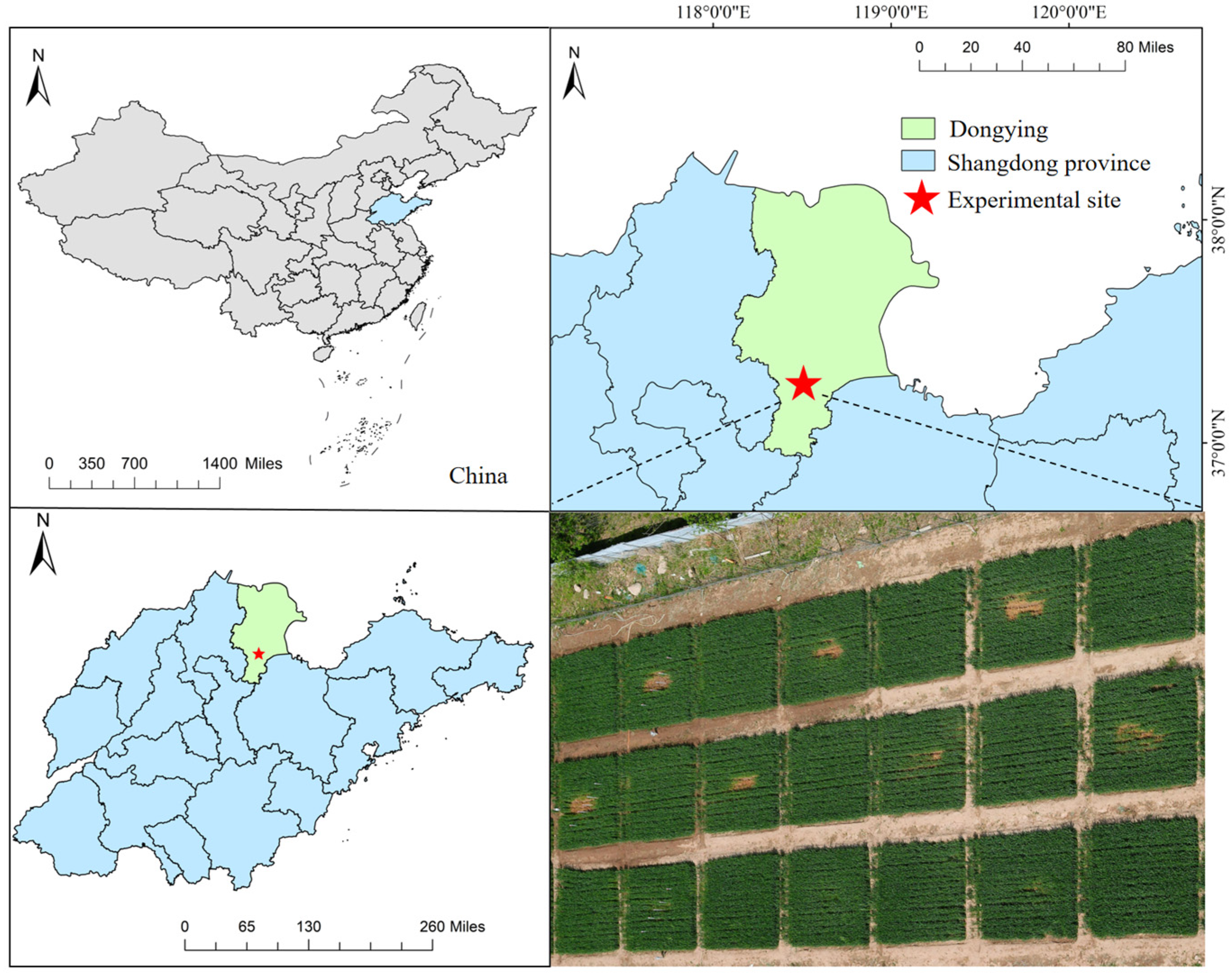
2.1. Study Area

The experiment was conducted in Dongying City (118°26′37.22″E, 37°25′16.54″N), Shandong Province, China, during the 2023–2024 winter wheat growing season, as shown in Figure 1. Dongying is located at a mid-latitude region, with a backland facing the sea, and has a warm-temperate continental monsoon climate with cold winters and hot summers and four distinct seasons.

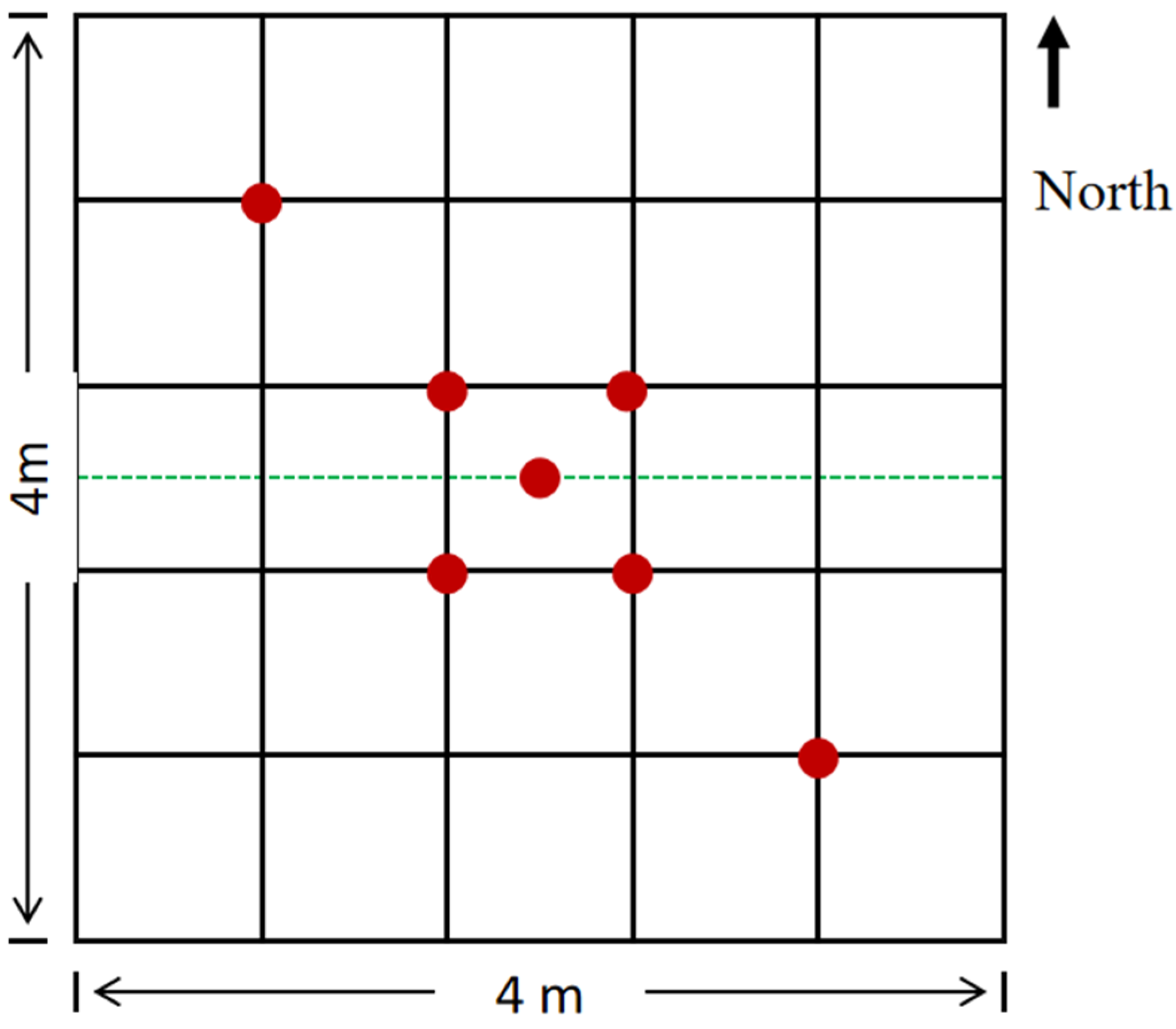
2.2. Experimental Field Design

In this study, four types of CO₂ stresses were used: normal environment (ctrl), 1 L/minute CO₂ stress (1 L stress), 3 L/minute CO₂ stress (3 L stress), and 5 L/minute CO₂ stress (5 L stress). Each CO₂ treatment consisted of four sample plots, for a total of 12 stress plots and 12 control plots. To verify the CO₂ stress in wheat at different growth stages, experiments were conducted at the joining (4 April), tasseling (16 April), flowering (9 May), and grouting (19 May) stages. Field management practices followed conventional local farming practices, including fertilizer application, drip irrigation, pest control, and weed management. The sown wheat grew normally, and field conditions were conducive.

CO₂ was injected into the experimental plot, and copper pipes were used for gas transportation, as shown in Figure 2. The PVC pipe was inserted into the center of the plot at a 30° angle from the northern edge to the vertical direction, reaching a depth of approximately 60 cm. At the pipeline’s end, 8 small holes were evenly created in various directions to ensure minimal gas leakage, with the CO₂ concentration at each leakage point in different directions being essentially the same. The holes were sealed with gauze to prevent soil blockage. The gas flow rate was remotely regulated by a Programmable Logic Controller (PLC), maintaining gas leakage rates of 1 L/minute, 3 L/minute, and 5 L/minute. Following the ventilation initiation, gas leakage was sustained for 24 h until the experiment’s completion. Wheat was uniformly sown in the plots, and CO₂ was injected into the experimental plots when vegetation growth was relatively stable. Throughout the experiment, both the control group and the experimental group underwent identical treatments to ensure normal plant growth conditions, with the only difference being the injection of CO₂ into the experimental group’s plots.

2.3. Data Acquisition

2.3.1. Soil Gas Concentration Measurement

The gas concentration in the soil of the experimental plots was measured using a GXH-3050E portable infrared gas analyzer produced by Beijing Tongde Venture Technology Co. (Beijing, China). Seven gas concentration sampling points were laid out in the experimental plot, and the sampling points were set up as shown in Figure 3. One hollow PVC pipe was inserted at each point, and the bottom end of each pipe was inserted into the soil at a depth of 30 cm from the surface, respectively. The top of the pipe was plugged with a rubber stopper to prevent gas diffusion from affecting the measurement of gas concentration. The rubber stopper was pulled out for observation and direct connection to the instrument during the measurement, and when the gas diffusion in the soil reached a stable state, the CO₂ concentration value at the point was measured at this time. Gas concentration data can be used to assist in verifying CO₂ leakage.

2.3.2. Spectral Measurement

Using an SVC HR-1024i spectrometer (Spectra Vista Corporation, Poughkeepsie, NK, USA), spectral data were collected from the wheat canopy. The spectrometer is capable of measuring UV, VIS, and NIR spectral bands within the range of 350–2500 nm, with 1024 bands, and a fiber optic field of view of 25 degrees. The instrument is equipped with three line array detectors. The bandwidth for the 350–1000 nm range is 1.5 nm, with a spectral resolution of 3.3 nm; the bandwidth for the 1000–1890 nm range is 3.8 nm, with a spectral resolution of 9.5 nm; and the bandwidth for the 1890–2500 nm range is 2.5 nm, with a spectral resolution of 6.5 nm. To ensure the accuracy and consistency of the data analysis, we resampled all the spectral data to 1 nm using the accompanying SVC professional software 7.1. All the spectral collection was carried out under clear and cloudless weather conditions, and the time was strictly controlled between 10 a.m. and 2 p.m. local time to minimize the influence of the variation of the sun’s altitude angle and the light conditions on the measurement results. Prior to the measurements, the instrument was strictly calibrated for reflectance using a standard plate to ensure the accuracy of the data [22]. Measurements were made with the operator wearing dark clothing, holding the probe at a height of approximately 1 m above the measurement point from the vegetation canopy, with the lens held vertically downwards, and with a field-of-view circle with a radius of approximately 22 cm. The canopy spectra of each plot were obtained from five different sampling points, and the average value was taken as the final spectral reflectance value, thus ensuring stability and reliability.

2.3.3. Measurement of Chlorophyll

The SPAD-502 chlorophyll meter produced by Minolta Camera Company of Japan uses the ratio of transmitted light in the 650 nm red light band and 940 nm near-infrared light band to measure the relative content of chlorophyll, and its SPAD value is dimensionless and has high correlation with the LCC; in this study, SPAD values were used instead of chlorophyll content. For the measurement, plants were randomly selected around the five sampling points in each plot, and measurements were taken in the middle of the second layer of leaves of each plant (starting from the top of the plant); five leaves were randomly selected at each point for measurement, the average of the measurements was taken as the SPAD value of the point, and the average of the SPAD values of the five sampling points was taken as the final LCC value of the plot. There were 48 control spectral samples and 48 stress spectral samples, and the number of chlorophyll data were the same as the number of spectral data. The data set of 96 samples was divided into 68 sample training sets and 28 sample test sets in a 7:3 ratio.

2.4. Methodologies

2.4.1. Fractional-Order Differentiation

In the field of vegetation spectral analysis, differential spectroscopy, as a widely used means of spectral curve transformation, focuses on the application of integer-order differentiation at its core. Although the method has multiple advantages, it ignores the critical fractional-order gradient information between the original spectra and the integer-order, which may lead to a bottleneck of accuracy when constructing the estimation model, limiting the accuracy of the overall analysis. In order to overcome this limitation, the theory of the FOD was developed, which, as a natural extension of integer-order differentiation, can capture the hidden details of the spectral data more finely, and effectively improve the efficiency of the use of hyperspectral information and the inversion accuracy of the vegetation parameters [23,24].

The FOD, which can essentially be regarded as a manifestation of arbitrary order derivatives of hyperspectral reflectance curves, is defined in various ways, mainly including the three classical forms of Grunwald–Letnikov, Riemann–Liouville, and Caputo. In view of the wide applicability of the Grunwald–Letnikov (G-L) method in practice, this method was chosen as an analytical tool in this study to dig deeper into the subtle features of wheat canopy spectra. On the MATLAB R2019b platform, we implemented a continuous differential transform from the 0th order to the 2nd order for the spectral reflectance of wheat using the 0.1 order as the incremental step. This strategy aims to fully explore the potential of the FOD technique in enhancing the accuracy of spectral analysis and provide strong technical support for the accurate inversion of vegetation parameters.

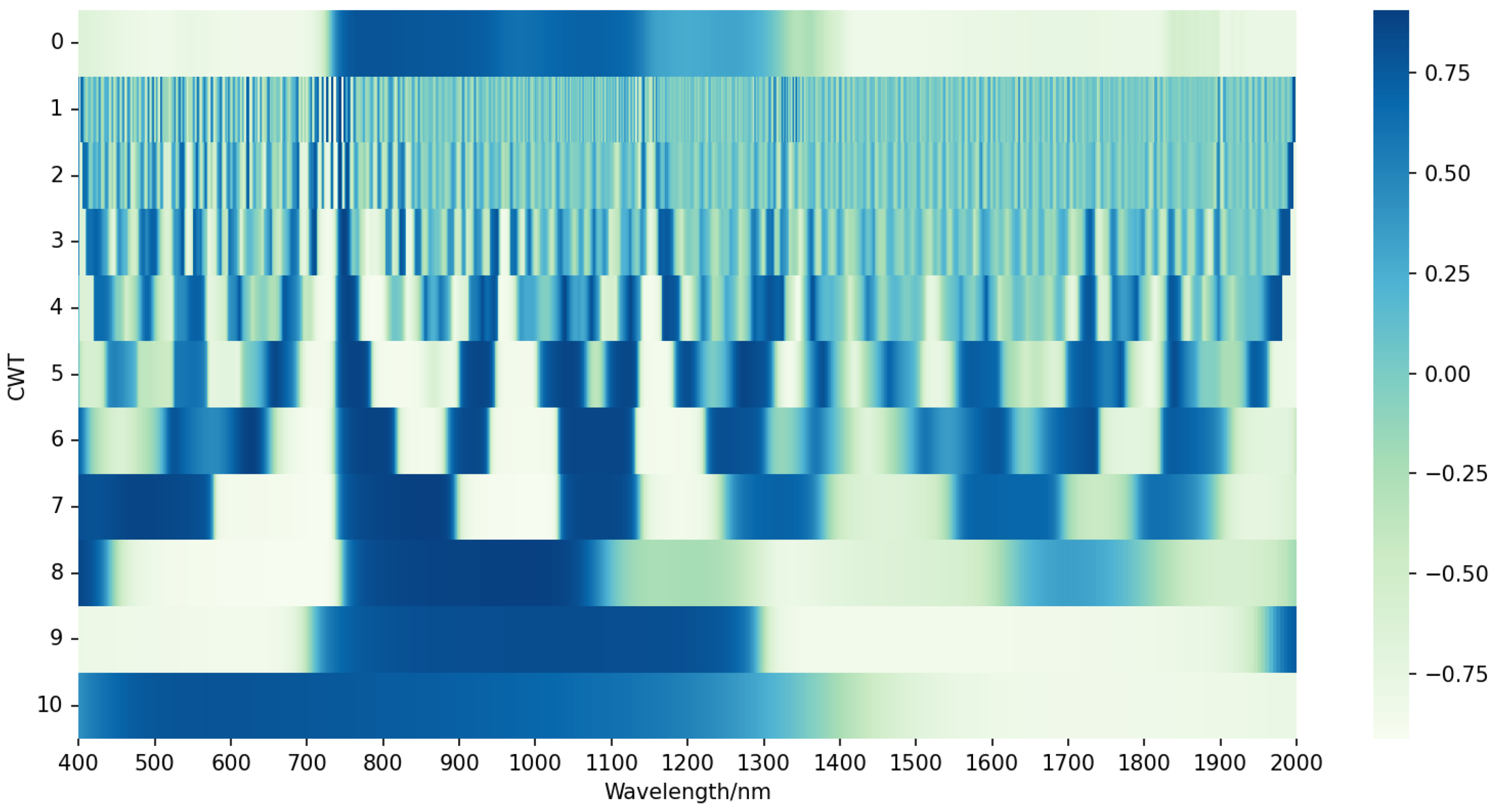
2.4.2. Continuous Wavelet Transforms

The CWT method, using a variety of wavelet basis functions, decomposes a complex signal into multiple wavelet components of different scales (or frequencies). This method is not only good at capturing the weak characteristics of the signal, but also significantly enhances the performance of local characteristics, reflecting its unique advantage for multi-scale analysis. The wavelet transform method is mainly divided into two categories: the CWT method and discrete wavelet transform (DWT) method. In this study, we adopt the CWT as an analysis tool to deeply analyze the hyperspectral data through the Gauss wavelet function. This process transforms the originally one-dimensional hyperspectral reflectance data into a two-dimensional matrix of wavelet coefficients, where the two dimensions correspond to the decomposition scale (from $i$ = 1 to $i$ = m, which is set to be from $2^1$ to $2^{10}$, i.e., from 1 to 10 scales, in this study) and the waveband (from $j$ = 1 to $j$ = $n$) [25].

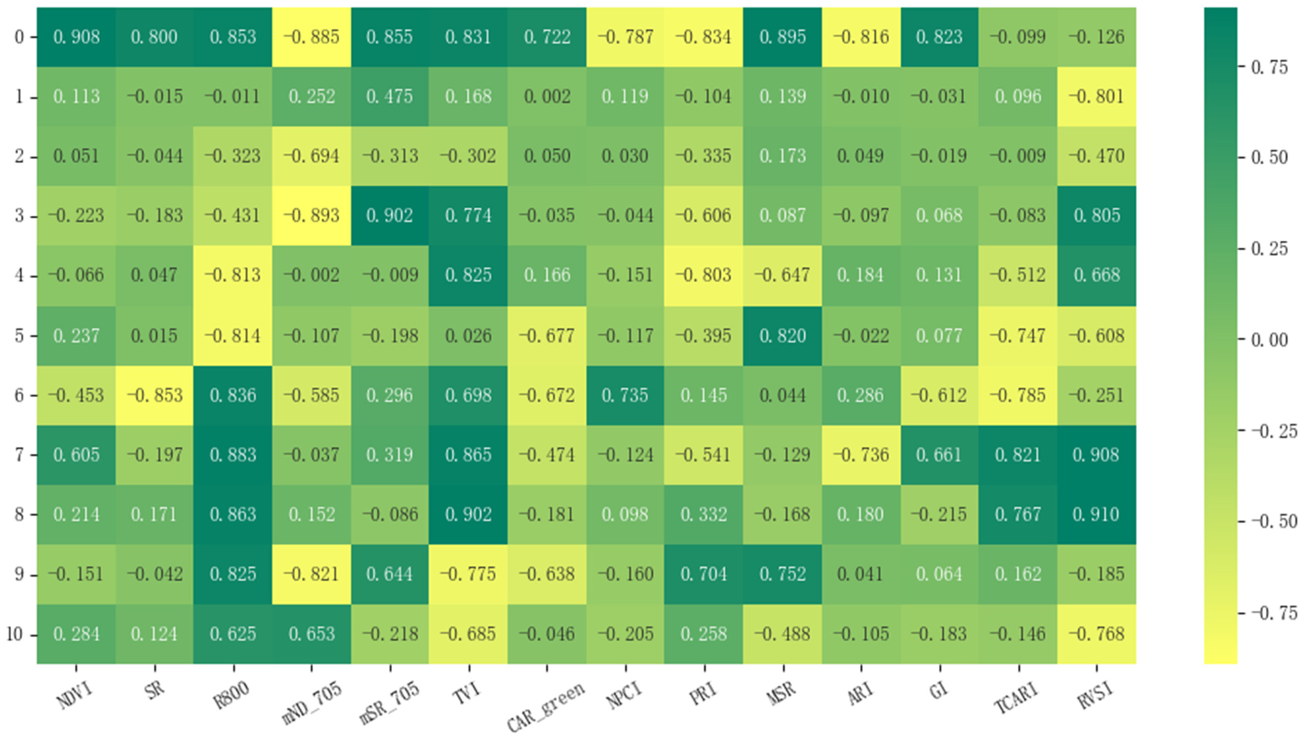
2.5. Constructing Multidimensional Vegetation Spectral Index

In order to efficiently identify sensitive spectral bands associated with the LCC under CO₂ stress from the FOD spectral data, we constructed difference (DVI), ratio (RVI), and normalized (NDVI) vegetation indices combining any 2 bands in the wavelength range of 400–2000 nm, which can simultaneously maximize the vegetation reflectance and minimize external influences [26].

$$NDVI=(R_i-R_j)\times {(R_i+R_j)}^{-1}$$

(1)

$$RVI=R_i\times {R_j}^{-1}$$

(2)

$$DVI=R_i-R_j$$

(3)

where $R$ is the spectral reflectance, $i$ and $j$ are any wavelengths in the range of 400–2000 nm, and $i\ne j.$

Through the application of the CWT method, we are not only able to decompose the spectral data and extract more detailed and differentiated spectral features, but also significantly amplify the subtle differences of the spectral curves at the key poles, which in turn enhances the sensitivity of detecting the subtle changes in the LCC under CO₂ stress. According to the hyperspectral characteristics of plants, various remote sensing vegetation indices are formed by combining visible and near-infrared bands. In this paper, 14 common vegetation indices were identified and calculated from the previous research work, as shown in

Table 1. Calculation of fourteen vegetation indexes using CWT-based spectral data.

Vegetation Indexes	Formulas	References
Normalized difference vegetation index (NDVI)	(R750 − R550)/(R750 + R550)	[27]
Simple Ratio (SR)	R800/R680	[28]
Color content index (R800)	R800 − R550	[29]
Modified normalized difference (mND 705)	(R700 − R705)/(R700 + R705 – 2 × R445)	[30]
Modified simple ratio (mSR_705)	(R750 − R445)/(R705 + R445)	[30]
Transformed Vegetation Index (TVl)	0.5 × (120 × (R750 − R550)) – 200 × (R670 − R550)	[31]
Green carotenoid index (CAR_green)	(1/R510 − 1/R550) × R770	[32]
Normalized chlorophyll ratio index (NPCI)	(R680 − R630)/(R680 + R630)	[33]
Photochemical vegetation index (PRI)	(R570 − R531)/(R570 + R531)	[29]
Improved odds index (MSR)	(R800/R670 − 1)/(R800/R670 + 1)	[31]
Anthocyanin reflectance index (ARI)	1/R550 − 1/R700	[34]
Greenness index (GI)	R554/R667	[29]
Corrective chlorophyll absorption odds Index (TCARI)	3 × (R700 − R675) − 0.2 × (R700 − R500) × R700/R670	[35]
Red-edged vegetation stress index (RVSI)	(R712 − R670)/2 − R732	[36]

.

2.6. Integrated Estimation Models

In this study, an integrated learning algorithm model is constructed based on the integrated learning idea of stacking. Stacking usually consists of two layers of learning networks: the first layer of the base model and the second layer of the meta-model. In the study, the predicted values of DTR, RF, and AdaBoost in the first layer of the base model are used as input features in the meta-model MLR to train the meta-model. In the base model, algorithms with large differences in principles are usually selected and cross-validated to fit that model.

2.7. Model Evaluation Methodology

In this study, the coefficient of determination ($R^2$), root mean square error ($RMSE$), and mean absolute error ($MAE$) were used as the main indicators to evaluate the predictive ability of each established model. The formulae are as follows:

$$R^2={\displaystyle \frac{{\sum }_{i=1}^n{\left(\widehat{y_i}-y_i\right)}^2}{{\sum }_{i=1}^n{\left(y_i-\overline{y}\right)}^2}}$$

(4)

$$RMSE=\sqrt{{\displaystyle \frac{1}{n}}{\sum }_{i=1}^n{\left(\widehat{y_i}-y_i\right)}^{2 }}$$

(5)

$$MAE={\displaystyle \frac{1}{n}}{\sum }_1^n\left|{\widehat{y}}_i-y_i\right|$$

(6)

where $\widehat{y_i}$ is the predicted value; $y_i$ is the observed value; $\overline{y}$ is the mean of the sample observations; $n$ is the total number of samples; and $i$ is the sample number.

3. Results

3.1. Dynamics of LCC Values in Wheat under CO₂ Stress

The variation in the LCC with the growth stage and aeration conditions of winter wheat is shown in Figure 4. The LCC values of CO₂-stressed wheat were all significantly smaller than those of control plants and decreased with the increase in the CO₂ aeration rate, and this pattern became more obvious as the reproductive period progressed. At the joining stage, the distribution of the LCC in the control and stressed plots was basically the same. From the joining stage to the grouting stage, the LCC of winter wheat in the control plots kept the trend of increasing and then decreasing, but the winter wheat in the stress plots kept decreasing, which might be related to the increase in CO₂. From the LCC of winter wheat leaves in the four fertility periods, it can be concluded that CO₂ had no effect on winter wheat leaves at the joining stage, began to appear at the tasseling stage, and had the greatest effect at the grouting stage.

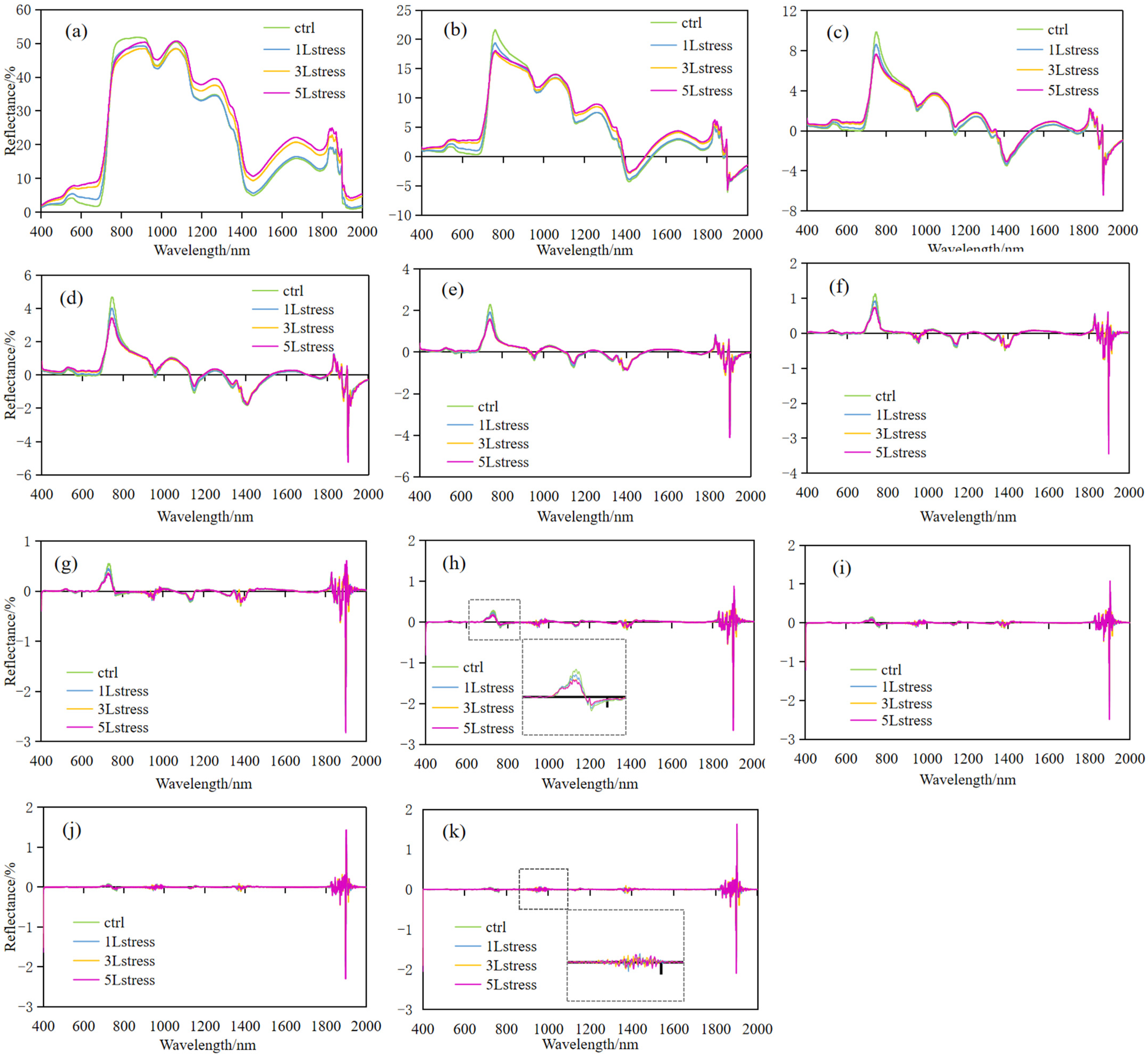
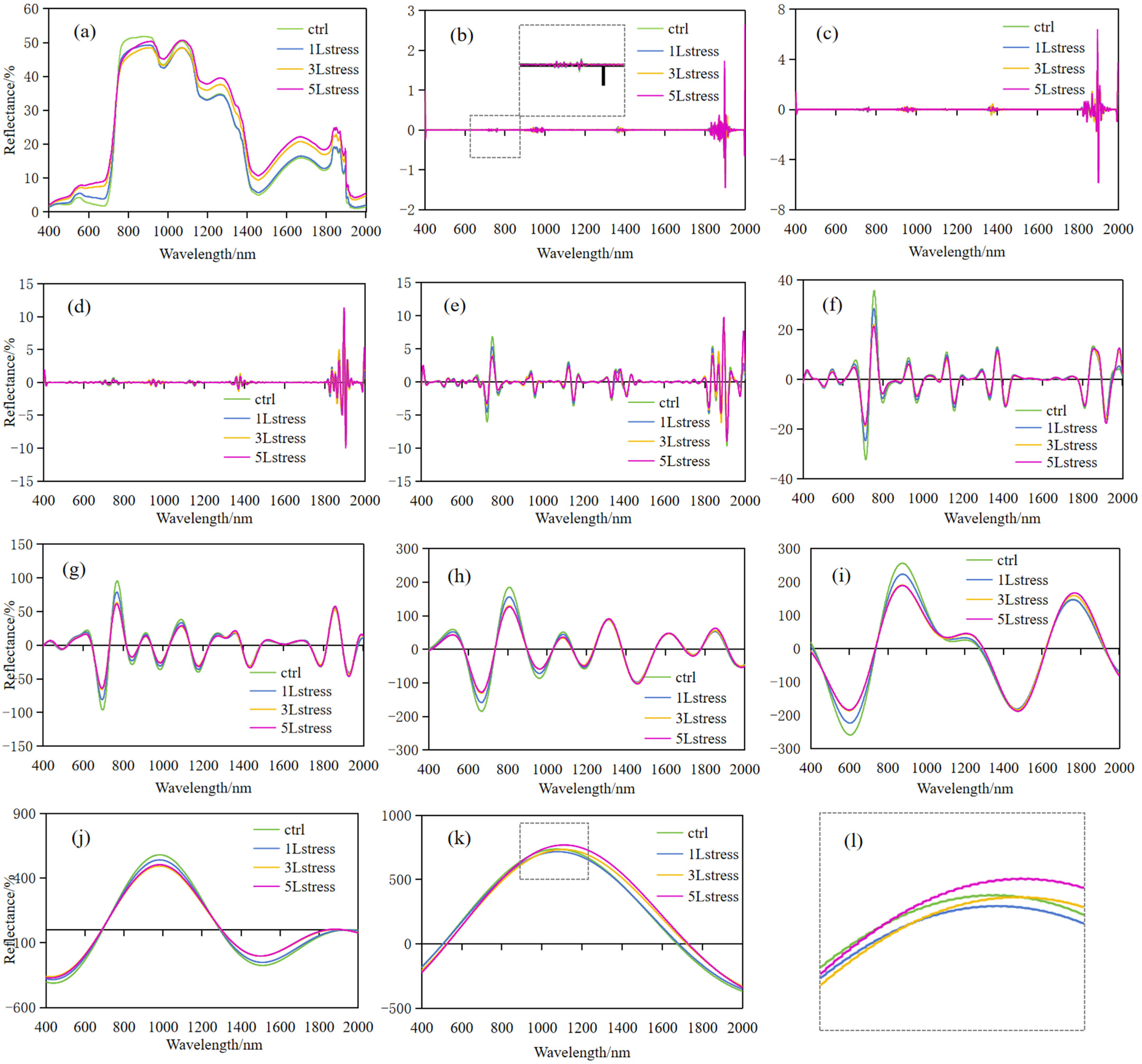
3.2. Dynamics of Reflectance Spectra of Wheat Canopies under CO₂ Stress

According to Figure 5, the spectral reflectance of winter wheat leaves showed a consistent pattern of spectral characteristics despite the variations at different growth stages. Specifically, in the visible region (400–780 nm), there are significant “green peaks” and “red valleys”, i.e., the spectral reflectance peaks in the green band at about 550 nm, and the reflectance troughs in the red band at about 680 nm. In the near-infrared band (780–1000 nm), the spectral reflectance of leaves increased sharply, and the increase was the most significant. Further analyses revealed that the effects of changes in the CO₂ aeration rate on the spectral characteristics of winter wheat leaves varied with the fertility period. At the joining stage, the spectral curves of both stress and control treatments almost overlapped, indicating that CO₂ changes had no significant effect on spectral characteristics at this stage. However, at the tasseling stage, CO₂ began to slightly affect the spectral reflectance of leaves in the near-infrared band, which showed a tendency of increasing reflectance in the stress group, marking the first appearance of CO₂ effects. At the flowering stage, the differences were more obvious, with the spectral reflectance of the wheat canopy in the control group generally higher than 0.4, while that of the CO₂-stressed treatment group was lower than this value. By the grouting stage, the spectral reflectance in the visible band increased in all treatments, and it was particularly noteworthy that the reflectance in the green peak region was not only enhanced under CO₂ stress, but also accompanied by the phenomenon of a “red shift”, i.e., the center of the green peak was shifted to the direction of the red light. Overall, the spectral reflectance in the visible band tended to increase with the increasing CO₂ aeration rate, while the spectral reflectance in the red and near-infrared bands weakened, and this trend was found in different reproductive periods, but the specific degree of the effect and the manifestation of the effect varied according to the growth period.

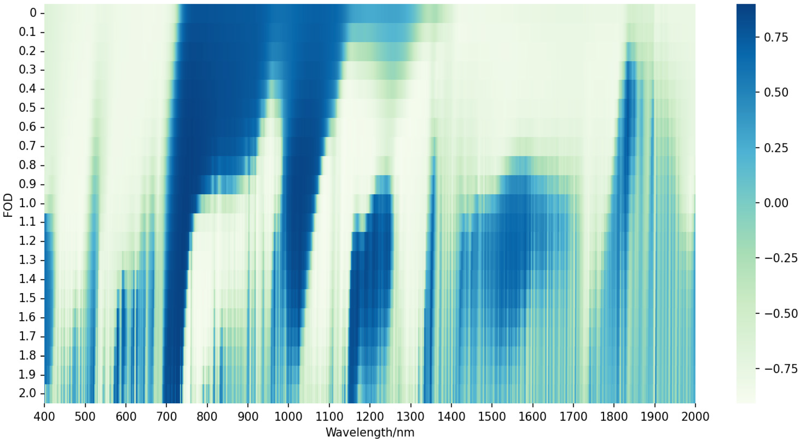
3.3. FOD-Based Analyses

In order to deeply investigate the specific effect of CO₂ on the spectral properties of winter wheat at the tasseling stage, we conducted a detailed hyperspectral analysis of wheat leaves at the tasseling stage, using the FOD method with a step size of 0.2, covering a range of orders from 0 to 2, and generating a total of 11 different differential transformation curves (shown in Figure 6). The analysis results showed that, regardless of the variation in the CO₂ stress rate, each differential curve followed a consistent pattern of change: the reflectance gradually decreased with the increase in the fractional order differential order, and finally converged to zero, and this trend clearly demonstrated the inverse relationship between the order and the reflectance.

In the spectral range of 400~1000 nm, we observe two significant reflection peaks, which are located in the green light band of 520~580 nm and the “red edge” band of 700~770 nm. The former originates from the specific reflection of green light during photosynthesis in green plants, while the latter is a typical sign of the sharp change in the spectral reflectance of green plants. It is worth noting that under CO₂ stress, the reflectance peaks in the 520–580 nm band were more significant than those of the control treatment, whereas in the 700–770 nm “red-edge” band, the reflectance of the control treatment was higher than that of the stress treatment, which highlights the significant effect of CO₂ on the spectral characteristics of wheat leaves during the tasseling stage.

When analyzing the correlation between the FOD bands and the LCC, we found a significant trend: the correlation coefficient R first showed an upward trend, followed by a gradual decrease (as shown in Figure 7 and

Table 2. Correlation coefficients between the optimized combination of bands with FOD and LCC.

FOD	Single Band	R	NDVI	R	RVI	R	DVI	R
original	R656	−0.840	(R721, R866)	−0.923	(R726, R851)	−0.923	(R730, R824)	−0.901
0.1	R1420	−0.845	(R717, R856)	−0.922	(R720, R851)	−0.921	(R723, R856)	−0.904
0.2	R764	0.842	(R716, R805)	−0.920	(R718, R806)	−0.919	(R716, R868)	−0.906
0.3	R763	0.859	(R730, R731)	−0.919	(R730, R731)	−0.919	(R699, R1062)	−0.905
0.4	R763	0.872	(R730, R731)	−0.919	(R730, R731)	−0.920	(R553, R1073)	−0.907
0.5	R762	0.882	(R518, R1042)	−0.921	(R721, R718)	0.921	(R553, R1055)	−0.918
0.6	R762	0.891	(R515, R1042)	−0.925	(R721, R717)	0.921	(R553, R1042)	−0.921
0.7	R762	0.898	(R510, R1041)	−0.928	(R722, R716)	0.922	(R506, R1073)	−0.925
0.8	R762	0.900	(R509, R1027)	−0.931	(R720, R524)	0.923	(R500, R1072)	−0.927
0.9	R752	0.895	(R508, R1027)	−0.933	(R720, R523)	0.927	(R504, R1028)	−0.924
1.0	R749	0.894	(R504, R1026)	−0.932	(R720, R523)	0.931	(R500, R1026)	−0.921
1.1	R1133	−0.893	(R504, R1026)	−0.930	(R720, R522)	0.933	(R499, R1028)	−0.916
1.2	R740	0.890	(R503, R1026)	−0.922	(R720, R522)	0.935	(R490, R1247)	−0.912
1.3	R826	−0.892	(R500, R1194)	−0.906	(R720, R522)	0.935	(R490, R1190)	−0.913
1.4	R826	−0.889	(R693, R734)	−0.900	(R720, R518)	0.933	(R490, R1190)	−0.914
1.5	R731	0.885	(R1900, R777)	−0.904	(R719, R518)	0.932	(R767, R1351)	−0.910
1.6	R756	−0.887	(R1900, R777)	−0.906	(R754, R518)	−0.930	(R767, R1351)	−0.913
1.7	R756	−0.895	(R1900, R755)	−0.902	(R754, R518)	−0.929	(R767, R1348)	−0.914
1.8	R755	−0.900	(R1899, R755)	−0.902	(R753, R518)	−0.922	(R755, R1168)	−0.913
1.9	R755	−0.906	(R727, R753)	−0.905	(R719, R509)	0.913	(R755, R1167)	−0.917
2.0	R755	−0.909	(R727, R753)	−0.913	(R750, R513)	−0.905	(R755, R1159)	−0.920

). In the raw spectral data without the FOD, the LCC showed a significant negative correlation, but in the specific wavelength range (700–1100 nm), this relationship was a significant positive correlation, especially at 656 nm, where the maximum negative correlation strength was reached (R = −0.84). The correlation pattern changed as the FOD level was increased. When the FOD level was increased to 0.4, the R-value in the 900–1000 nm band started to decrease, and a peak of negative correlation was observed. When further increased to level 0.9, the correlation coefficient in the 1100–1300 nm interval was significantly enhanced, while the number of positive correlation peaks gradually increased in the 1400–2000 nm range. When the FOD reaches level 1.1, the correlation is characterized by more complexity, especially at 1133 nm, where the R-value reaches a new maximum negative correlation (−0.893), while signs of positive correlation begin to appear near 700 nm and 1000 nm. Moreover, the R-value gradually decreases in the wavelength range of 1400–2000 nm. When the FOD is elevated to 2.0, the correlation between the spectra and LCC exhibits multiple significant positive and negative correlation peaks, with the largest negative correlation (R = −0.909) occurring at 755 nm, which further reveals the effect of the FOD on the spectral properties and their relationship with LCC.

To optimize the ultra-high dimensional features constructed under the FOD method to fit the LCC inversion requirements, we deeply explored and screened the feature combinations with the best correlation coefficients, R, in depth. As shown in Table 2, our analysis reveals that in the single band, the optimal performance is exhibited at 755 nm with an R-value of −0.909, which is ranked at order 2.0. Further, in exploring of dual-band combinations, we find that the correlation with LCC values can be significantly enhanced at specific orders (e.g., 0.9, 1.2, and 0.8). Specifically, the NDVI reaches an R-value of −0.933 at the 0.9 order, the RVI even reaches the highest R-value of 0.935 at the 1.2 order, while the DVI performs well at the 0.8 order with an R-value of −0.927. These results indicate that the dual-band combination strategy significantly enhances the correlation between the spectral data and LCC. Particularly noteworthy is that the RVI based on the principle of difference ratio stands out in the screening and exhibits the highest R-value, which emphasizes the importance of the information on the differences between the dual bands for enhancing the accuracy of LCC inversion. Through the in-depth analysis of the wavelength distribution of these efficient dual-band combination variables, we found that their wavelengths were mainly concentrated in the key spectral regions of 500 nm, 720 nm, 750 nm, and 1100 nm, which may contain the most sensitive information about the physiological state of vegetation.

3.4. CWT-Based Analysis

In order to study the effect of the CWT on the spectral curves of wheat leaves under stress, we performed 10 scale transformations using the CWT for the tasseling stage. Figure 8 clearly shows that after CWT decomposition, it can be seen that the wavelet coefficient values are both positive and negative, and there are more peaks and troughs in the wavelet curves of scales 4, 5, 6, and 7, indicating that this scale contains too much tiny information and noise, and the spectral changes of the stress and control groups are very drastic, and the spectra of the wheat leaf blades are significantly different between the control and the stress conditions, with the spectra of the different stresses in the ranges of 650–780 nm, 940- 970 nm, 1110–1180 nm, 1340–1420 nm, and 1800–2000 nm total five band intervals with large fluctuations in amplitude values and some differences. With the increase in the decomposition scale, the absorption and reflection spectral properties in this range tend to increase and then decrease. In addition, the absorption valley and reflectance peaks are sharpest when the CWT is at scale 5, and then gradually smoothed. The scale 1, 2, and 3 reflectance values are close to 0, because the high-frequency wavelet can extract subtle features and rapidly changing components in the signal. However, the high-frequency signal consists mainly of noise which affects the extraction of effective information. Due to the significant reduction in the wavelet center frequency, the CWT extracted more low-frequency signals from the leaves from scale 8 onwards, resulting in smoother spectral curves.

Figure 9 reveals the effect of the CWT method in processing the hyperspectral characteristics of wheat leaves under CO₂ stress, especially in transforming the significant positive and negative correlations in the original spectra into a more detailed positive and negative alternating pattern. This transformation demonstrates that the CWT method can accurately capture and extract the edges, transitions, and details of different chemical elements in the spectral signals, especially in the scale interval from 1 to 5, effectively decomposing the overlapping peaks of the spectra and improving the value of the correlation coefficient R. The CWT method not only strengthens the correlation between the spectral data and the LCC values, but also improves its correlation. As shown in

Table 3. Optimal correlation coefficients between CWT spectra and LCC at different scales.

CWT	Origin	1	2	3	4	5	6	7	8	9	10
band	656	737	738	749	788	764	626	720	708	1388	1727
R	−0.840	−0.878	−0.873	0.890	−0.891	0.884	0.901	−0.909	−0.911	−0.857	−0.837

, at scale 1, the R-value reaches a local high point at 737 nm (−0.878), while at scale 8, the maximum R-value is elevated to −0.911, occurring at 708 nm, which is a significant increase (by 0.071) compared to the R-value of the original spectrum (−0.84). This trend shows that with the change in the scale, the R-value exhibits the characteristic of enhancing and then slightly decreasing, reflecting the balance between the fineness of information extraction and the optimization of the correlation at different scales. It is worth noting that the R-value decreased when the scale was increased to 9 and 10, which may be due to the decrease in the wavelet center frequency, resulting in a weaker ability to characterize the fine absorption features and leaf structural features in the original reflectance spectra, further reflecting the wider range of features. In summary, the application of the CWT method in wheat leaf hyperspectral data provides a powerful tool for the in-depth analysis of spectral data by effectively extracting the LCC sensitive bands.

In order to extract the LCC-sensitive vegetation indices in the CWT, correlation analyses of vegetation indices at different CWT scales were performed in this study. As shown in Figure 10, most of the R-values based on the original band vegetation index values approximated 0.8, and the NDVI had the highest R-value (R = 0.908) among the original spectral-based vegetation indices. However, the TCARI and RVSI had lower R-values, indicating that not all vegetation indices reflect the LCC of the raw hyperspectral data well. Most of the vegetation indices improved in different components based on the CWT decomposition, with R > 0.85 concentrated in scale 7 and 8. Scale 8_RVSI had the highest correlation coefficient with R = 0.910.R800 on the scale of 1–7. There was an increasing trend, with the highest R-value for this vegetation index (R = 0.883) being achieved on scale 7. mSR_705, TVI, TCARI, and RVSI significantly improved the R-value, with the RVSI increasing from −0.126 to 0.910. However, the R-value of the NDVI declined after the CWT treatments, with the R-value falling below 0.453 on scales 1–6, and reaching 0.605 on scale 7. This may be due to the fact that some of the vegetation indices take into account the effects of the broad absorptive properties of the leaves and leaf structure. Overall, the correlation coefficients between some of the vegetation indices and the LCC were significantly higher after treating the raw spectra with the CWT method.

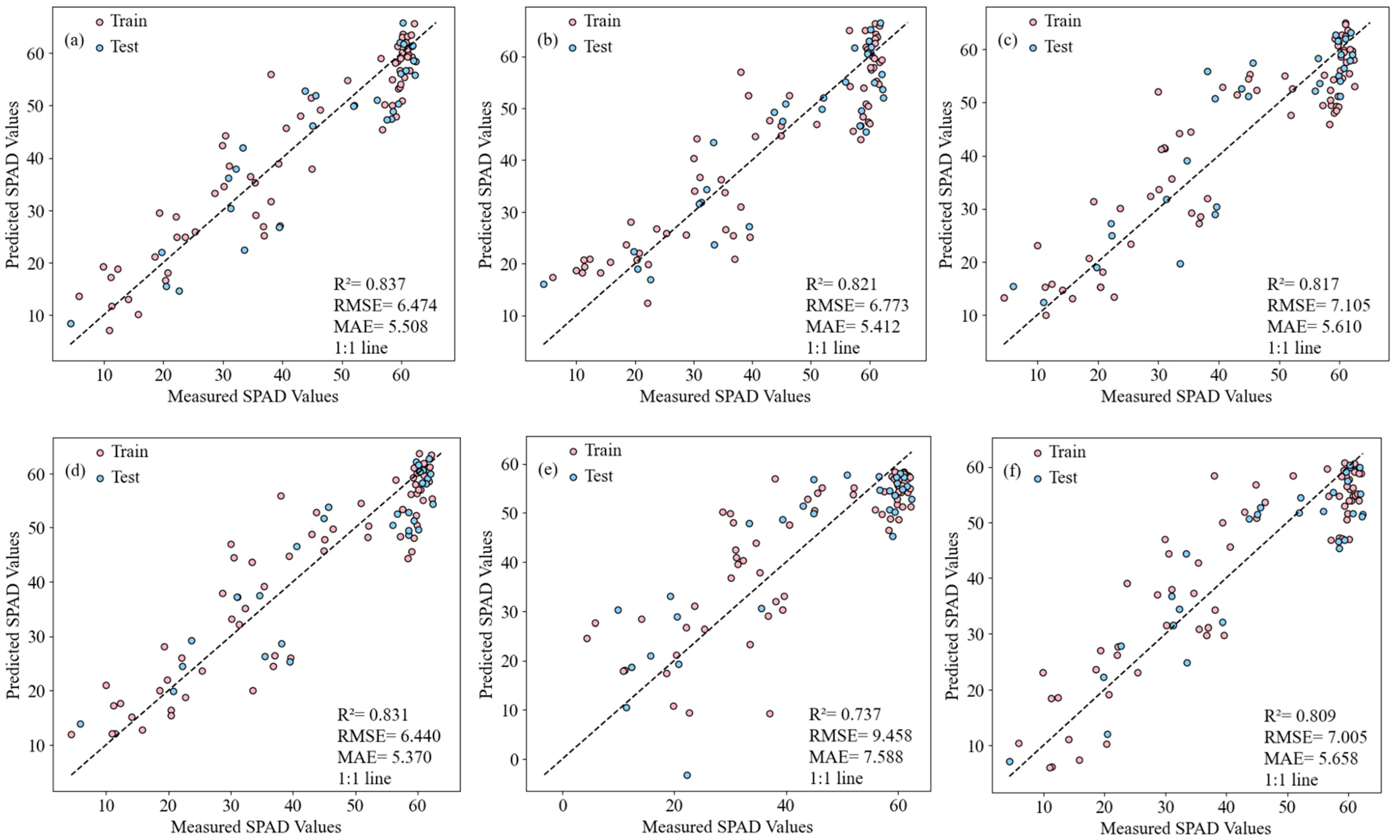
3.5. Comparison of LCC Estimation Based on FOD, CWT, and Raw Spectral Features

Based on the above exhaustive analyses, we carefully screened specific bands and indices with a high correlation with LCC values under raw spectra, FOD, and CWT treatments, and the specific results are shown in

Table 4. Selected MLR modeling features.

	Original	FOD/CWT
Single band	R656 = −0.840	R755 = −0.909
Dual band	NDVI (R721, R866) = −0.923	RVI (R720, R522) = 0.935
Vegetation index	NDVI = 0.908	RVSI = 0.910

. In the field of raw spectra, a significant correlation of −0.840 was demonstrated at 656 nm in the single band, and a high correlation of −0.923 was achieved on the dual-band combination (R₇₂₁, R₈₆₆), while the NDVI also stood out with its correlation of 0.908. Turning to the FOD treatment, the single band reaches a correlation of −0.909 at order 2.0, while the dual band performs the best on the RVI (R₇₂₀, R₅₂₂) at order 1.2. Meanwhile, the RVSI under the CWT treatment exhibited the highest correlation (0.910).

Subsequently, we performed MLR modeling using these selected feature variables and evaluated the accuracy performance of the features on the validation set under different treatments (shown in Figure 11). The overall trend showed that the vegetation spectral indices constructed from the dual-band combination achieved the optimal prediction accuracy on the validation set for both raw and FOD spectra, closely followed by the vegetation indices under the CWT treatment. In contrast, the single band in the raw spectra performed well (R² = 0.737, RMSE = 9.458, MAE = 7.588 for the training set), but its accuracy was relatively weak. Particularly notable is that the NDVI variable selected from the 1.2 order arbitrary two-band combination achieved the best prediction accuracy in the validation set (R² = 0.837, RMSE = 6.474, MAE = 5.508), a result that is a significant improvement over the single-band and band-specific vegetation index feature variables.

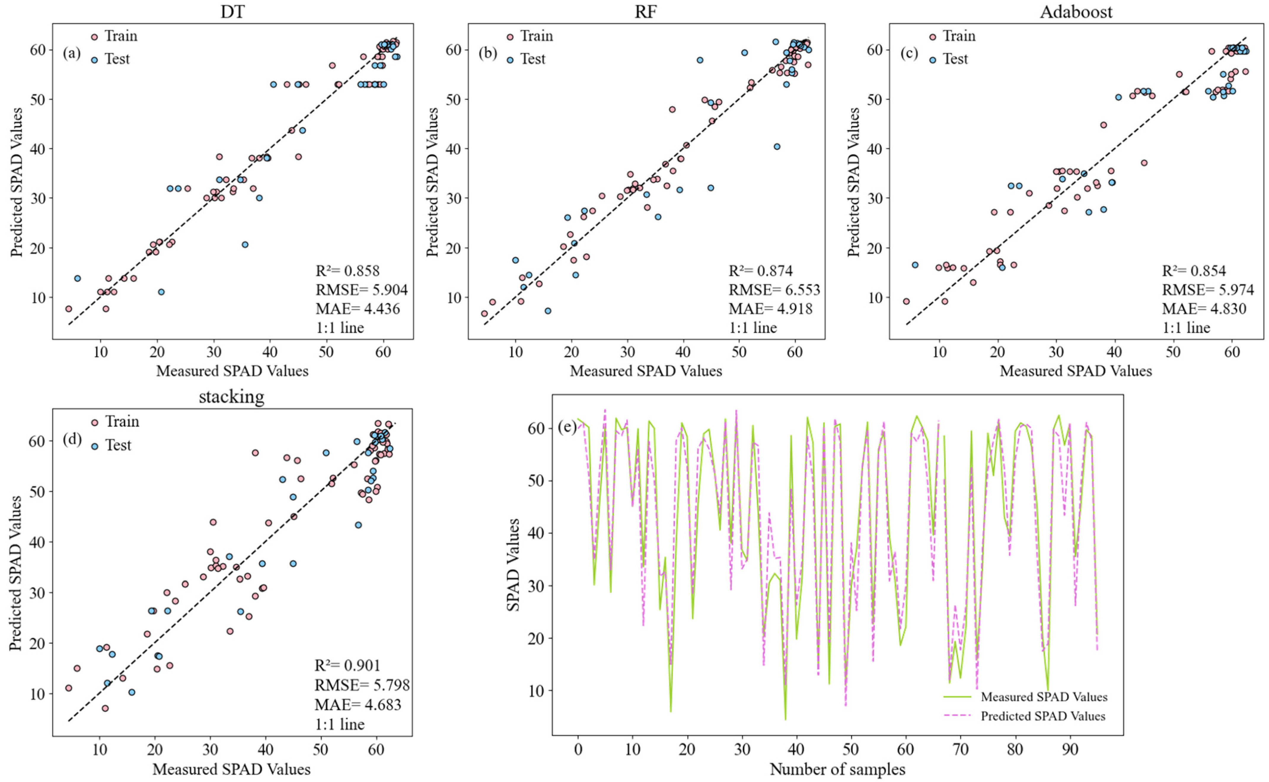
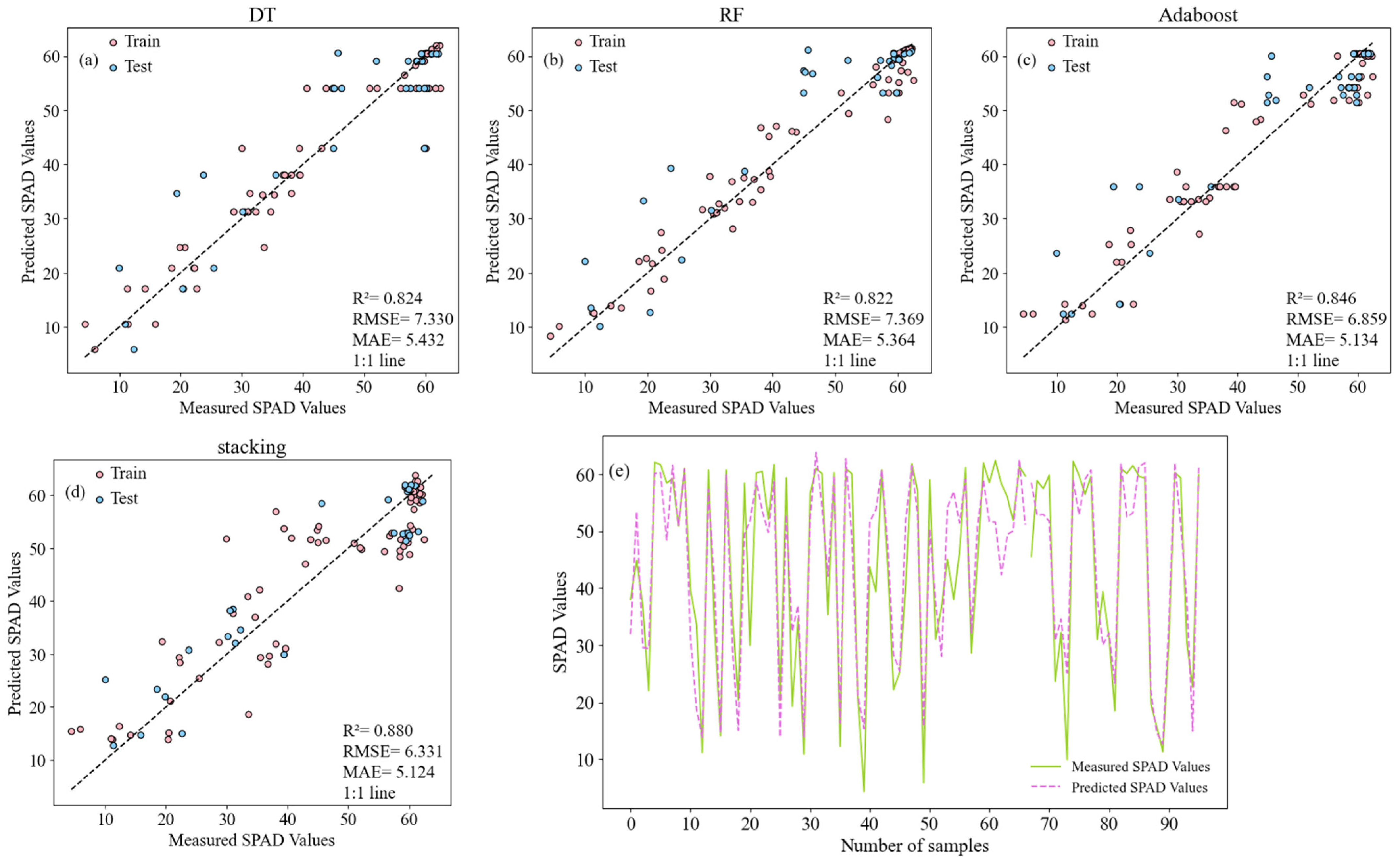
3.6. FOD-Based LCC Estimation

In this study, the stacking integrated model was applied to accurately estimate the LCC of wheat in combination with the RVI of the 1.2th order derivatives, which was carefully screened based on Pearson correlation analysis. As shown in Figure 12a–d, the stacking model and its three sub-models performed excellently on the test set, with R² values all stable above 0.854, a result that strongly demonstrates the effectiveness of the FOD-transformed dual-band vegetation spectral index as a predictor of the LCC for wheat. Particularly noteworthy is that the stacking approach, by incorporating multiple sub-models, achieved the highest prediction accuracy (R² = 0.901, RMSE = 5.798, MAE = 4.683), which was significantly better than the DTR and Adaboost models alone, which had R² values of 0.858 and 0.854, respectively; even though the DTR model had a slightly lower MAE than the stacking model (0.247 lower), the overall performance is still inferior to the stacking model. Figure 12e visualizes the close correspondence between the predicted and measured LCC of the stacking model, and the comparison shows that the model-predicted leaf LCC is highly consistent with the measured values, which further verifies the high efficiency and accuracy of the 1.2-order derivative RVI vegetation spectral index constructed based on the FOD transform method for estimating the LCC of wheat.

3.7. CWT-Based LCC Estimation

In this study, the stacking integrated model was used in conjunction with the scale8_RVSI features preferred by the correlation analysis to accurately estimate the LCC of the leaves. As shown in Figure 13a–d, the stacking model and its three constituent sub-models all performed very well on the test set, with their R² value remaining above the level of 0.822. In particular, the stacking integrated model significantly improves the prediction accuracy as demonstrated by the further optimization of R² = 0.880, RMSE = 6.331, and MAE = 5.124. In contrast, of the three sub-models, the RF, although robust, was slightly less accurate (R² = 0.822, RMSE = 7.369, MAE = 5.364), while the AdaBoost model demonstrated the highest single-model accuracy (R² = 0.846, RMSE = 6.859, MAE = 5.134). Figure 13e visually reveals the close relationship between the predicted and measured LCC values of the stacking model, and the comparison reveals a high degree of consistency between the predicted and measured values of the model, which fully validates the accuracy and reliability of the stacking model in the estimation of LCC.

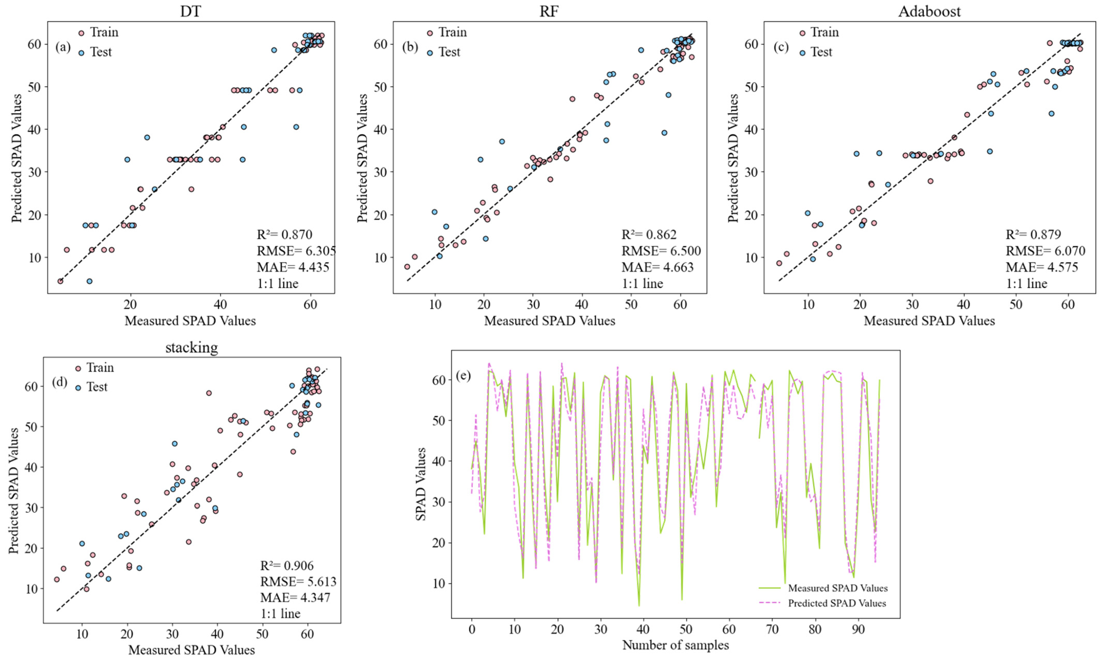
3.8. LCC Estimation Based on the Combination of FOD and CWT

Figure 14a–d demonstrate the accuracy performance of the 1.2-order derivative RVI and cwt8_RVSI in LCC estimation. Notably, the stacking integrated model exhibits the optimal prediction performance, closely followed by the Adaboost model with key performance metrics including R² = 0.879, RMSE = 6.070, and MAE = 4.375. The experimental result clearly reveals that compared to using either feature alone, the combination of the 1.2-order RVI with the scale8_ RVSI’s clever fusion brings a significant accuracy improvement. Specifically, the combined feature was tested with an accuracy of R² = 0.906, an improvement of 0.005 compared to the 1.2-order RVI alone (R² = 0.901), while a significant improvement of 0.026 was achieved compared to the scale8_RVSI alone (R² = 0.880). This finding strongly demonstrates that the optimal combination of FOD-based features with CWT features can effectively enhance the accuracy of a single feature in predicting the LCC.

Further, the prediction accuracies of various machine learning models such as stacking, DTR, RF, and Adaboost are significantly enhanced by this feature combination. Figure 14e visually demonstrates the high degree of consistency between the predicted and measured LCC of the stacking model, and although there is still a slight deviation, this deviation has been significantly reduced compared to the results in Figure 12e and Figure 13e, which signals a significant improvement in the model performance. This finding suggests that by jointly utilizing the RVI and cwt8_ RVSI for the co-estimation of LCC, not only can the estimation accuracy be improved, but the robustness and generalization ability of the model are also enhanced. In summary, compared with the application of a single feature, the integrated inversion strategy of the 1.2-order RVI and cwt8_RVSI undoubtedly opens up a more efficient and reliable pathway for accurate LCC measurements.

4. Discussion

The spectral properties of plants, as a visual reflection of the chemical and physiological state of leaves, show a high degree of sensitivity to environmental changes. This study revealed that the spectral response of wheat was significantly affected by CO₂ leakage in the visible region of 450–680 nm, a finding that coincides with the spectral response patterns of soybean, alfalfa, and barley under similar soil CO₂ stress conditions [37,38,39]. Within this spectral range, the variation in the content of chlorophyll, the dominant pigment, is particularly critical because it is responsible for absorbing most of the visible energy, especially in the 450–680 nm band [40]. Therefore, the spectral reflectance in this band becomes a sensitive indicator to monitor the dynamic changes of chlorophyll. Further analyses showed that two specific bands, 552–554 nm and 667–674 nm, were particularly responsive to high CO₂ concentrations in the soil in the raw spectra of wheat, and these bands happened to be located within the aforementioned key visible light regions. This reinforces the value of the application of spectral analysis in monitoring changes in plant physiological state under CO₂ stress. Studies such as the work of Al-Traboulsi et al. [1] have shown that soil CO₂ stress inhibits plant growth, and this effect is closely related to changes in the spectral characteristics of the plant, as evidenced by a decrease in the content of photosynthetic pigments, such as chlorophylls and carotenoids [41,42,43]. This experiment also verified this conclusion through the significant decrease in the LCC, which visually demonstrated the negative effect of soil CO₂ stress on wheat growth. In summary, the spectral analysis technique provides a powerful tool for an in-depth understanding of the mechanism of CO₂ leakage on plant growth.

In addition, the FOD and CWT methods can be utilized to refine spectral curve trends and features, including peak and valley wavelengths. The FOD and CWT methods have been proposed as a means of eliminating sources of variability associated with broadband ratios, providing more sensitive stress measurements compared to raw spectral data. This study showed that FOD reflectance in the 541–544 nm and 746–748 nm bands had significant leakage in response to CO₂ and showed distinct peaks (Figure 3). Notably, the peaks and troughs of the spectra rose and fell with increasing concentrations of soil CO₂. Based on this, two parameters, the 1.2-order RVI and CWT_8RVSI, were effectively extracted and used in the subsequent construction of the LCC estimation model.

This study discovered that based on the datasets of the 1.2-order derivative RVI (R² = 0.901, RMSE = 5.798, MAE = 4.683), scale8_RVSI (R² = 0.880, RMSE = 6.331, MAE = 5.124), and the 1.2-order derivative RVI and scale8_RVSI (R² = 0.906, RMSE = 5.613, MAE = 4.347), the stacking model demonstrated superior estimation performance for LCC. The results suggested that the stacking model, through integrating multiple sub-models, could attain the high-precision estimation of LCC under CO₂ stress. Considering the influence of CO₂ stress on the canopy structure and physiological characteristics of plants, those features capable of responding to the stress are also likely to be employed for estimating the LCC under stress. Hence, this study aimed to explore the features sensitive to chlorophyll changes under different CO₂ stresses and utilize these features to precisely estimate the LCC under stress, thereby providing a scientific basis for timely management measures.

In the expansive domain of exploring LCC estimation, despite numerous research contributions, the estimation outcomes among different methods exhibit considerable disparities and uncertainties. This phenomenon is especially salient in the comparison of the three stacking models depicted in Figure 15. Specifically, the scale8_RVSI model displays substantial bias fluctuations, revealing its inherent instability and high uncertainty in predicting the LCC under CO₂ stress. In contrast, the strategy that integrates the 1.2-order derivative RVI and cwt8_CI_RVSI model, through the ingenious combination of FOD and CWT sensitivity, showcases a more resilient and precise prediction performance, pioneering a novel approach to enhance the accuracy and stability of LCC estimation. Through an in-depth analysis of the data in Figure 14 and Figure 15, it is not arduous to discover that there are certain underestimation phenomena in this study, accompanied by a high deviation value, which might be intimately associated with the under-representation of sampling points and the complexity and variability of the local terrain [26]. Generally speaking, the uncertainty of wheat LCC estimation ought not to be disregarded, and its origin could be traced back to the diversity of the LCC measurement data itself. As the basis of the evaluation, the abundance and quality of samples are directly correlated with the accuracy of the estimation. Therefore, enhancing the regional representation of sampling points and optimizing the standardization of sampling techniques, processes, and experimental operations have emerged as the key to reducing uncertainty and improving data reliability [44]. Of particular note is the maximum deviation of 20 SPAD presented in Figure 15b, a significant deviation that can be attributed to minor errors in the LCC measurement process, encompassing but not limited to minor alterations in equipment accuracy, operating specifications, or environmental conditions. In light of this, the emphasis on the high degree of uniformity and standardization of sampling and experimental procedures is invaluable in minimizing such errors and guaranteeing data quality.

The study’s main shortcomings are the limited scope of the experimental subjects, the narrow range of stress types, the short time scale, and the constraints on the sample size and geographic coverage. These factors collectively restrict the broad applicability of the research findings and the generalizability of the model. Specifically, the study’s focus on the hyperspectral characterization of winter wheat under CO₂ stress overlooks the complexities of multi-species, mixed vegetation, and other environmental stressors (such as ozone, warming, moisture, and salinity). The data collection is confined to a single-year wheat growth cycle, with an inadequate sample size and limited geographic representation, potentially compromising the model’s stability and reliability under varying environmental conditions.

Looking ahead, to address these limitations, the study should be expanded to include more plant species and vegetation types. It should explore the spectral characteristics of mixed vegetation under CO₂ stress and conduct comprehensive analyses in conjunction with various environmental stressors to uncover the spectral response mechanisms of crops under complex environmental conditions. Simultaneously, a long-term and continuous observation system should be established to identify the specific bands and indicators of CO₂ stress by accumulating and analyzing years of data, thereby enhancing the stability and reliability of the model. Furthermore, by integrating remote sensing technology and ground observation data through multi-scale analysis and model optimization, the study aims to delve into the influence mechanism of CO₂ stress at different spatial scales and enhance the prediction accuracy and robustness of the model. Lastly, interdisciplinary collaboration will be strengthened, and new technologies such as drones, the Internet of Things, and artificial intelligence will be utilized to drive innovation and advancement in crop stress monitoring technology, offering more convenient and efficient solutions for agricultural production.

5. Conclusions

In this study, a new breakthrough was made in the field of estimating the LCC of wheat leaves under stress conditions. An efficient estimation method was constructed by integrating raw hyperspectral data, stacking the integrated learning regression model, and FOD and CWT spectral processing techniques. In this study, we carried out an in-depth fine analysis of the spectral response of wheat leaves, and accurately identified the key spectral characteristic variables affecting the LCC under stress conditions. The performance of the optimal spectral feature combinations after the FOD and CWT treatments in LCC estimation was systematically evaluated, and the study not only confirmed that the combination of FOD and CWT techniques could significantly enhance the sensitivity of spectral data to LCC changes under stress, but also verified the effectiveness of the integrated method in improving the accuracy of LCC estimation. The conclusions are as follows:

• Under CO₂ stress conditions, the hyperspectral features of winter wheat changed significantly, as evidenced by the decrease in the LCC with the enhancement of stress, the enhancement of the reflectance of the green peak of the hyperspectral curve with the red shift, and the blue shift of the red edge, which accurately revealed the impact of CO₂ on wheat physiology, and provided the scientific basis and technical support for the monitoring of the impact of large-scale CO₂ on wheat yield by using the key spectral features of the band to assist in the precise management of agricultural responses to climate change.
• The effectiveness of the FOD and CWT spectral processing methods in weakening the baseline drift and overlapping peaks of the original spectra and enhancing the correlation between spectra and physiological indicators was also validated under CO₂ stress conditions. This implies that these techniques are not only applicable to LCC estimation under normal growth conditions, but also can effectively support the accurate estimation of LCC under CO₂ stress.
• The FOD-based dual-band combination is superior to the single band and can significantly improve the prediction of the LCC. The 1.2-order derivative dual-band RVI (R₇₂₀, R₅₂₂) showed excellent prediction ability under CO₂ stress conditions (R² = 0.901, RMSE = 5.798, MAE = 4.683), which realized a high precision estimation of the LCC.
• The application of CWT multi-scale analysis under CO₂ stress has also achieved remarkable results. By analyzing the spectral data at different scales, we constructed the RVSI, which can reflect the effects of CO₂ stress and achieve a reliable estimation of LCC (R² = 0.880, RMSE = 6.331, and MAE = 5.124). The combination of sensitive spectral features based on FOD and CWT techniques enhances the estimation accuracy of LCC estimation under the stacking model (R² = 0.906, RMSE = 5.613, MAE = 4.347).

References

1. Al-Traboulsi, M.; Sjögersten, S.; Colls, J.; Steven, M.; Craigon, J.; Black, C. Potential Impact of CO2 Leakage from Carbon Capture and Storage (CCS) Systems on Growth and Yield in Spring Field Bean. Environ. Exp. Bot. 2012, 80, 43–53. [Google Scholar] [CrossRef]
2. Shang, Y.; Chen, X.; Yang, M.; Xing, X.; Jiao, J.; An, G.; Li, X.; Xiong, X. Comprehensive Review on Leakage Characteristics and Diffusion Laws of Carbon Dioxide Pipelines. Energy Fuels 2024, 38, 10456–10493. [Google Scholar] [CrossRef]
3. Kim, Y.J.; He, W.; Ko, D.; Chung, H.; Yoo, G. Increased NO2 Emission by Inhibited Plant Growth in the CO2 Leaked Soil Environment: Simulation of CO2 Leakage from Carbon Capture and Storage (CCS) Site. Sci. Total Environ. 2017, 607–608, 1278–1285. [Google Scholar] [CrossRef] [PubMed]
4. Zhang, X.; Ma, X.; Wu, Y.; Li, Y. Enhancement of Farmland Greenhouse Gas Emissions from Leakage of Stored CO2: Simulation of Leaked CO2 from CCS. Sci. Total Environ. 2015, 518–519, 78–85. [Google Scholar] [CrossRef]
5. Zhou, X.; Lakkaraju, V.R.; Apple, M.; Dobeck, L.M.; Gullickson, K.; Shaw, J.A.; Cunningham, A.B.; Wielopolski, L.; Spangler, L.H. Experimental Observation of Signature Changes in Bulk Soil Electrical Conductivity in Response to Engineered Surface CO2 Leakage. Int. J. Greenh. Gas Control 2012, 7, 20–29. [Google Scholar] [CrossRef]
6. Feitz, A.; Jenkins, C.; Schacht, U.; McGrath, A.; Berko, H.; Schroder, I.; Noble, R.; Kuske, T.; George, S.; Heath, C.; et al. An Assessment of near Surface CO2 Leakage Detection Techniques under Australian Conditions. Energy Procedia 2014, 63, 3891–3906. [Google Scholar] [CrossRef]
7. Wang, P.; Xu, Y.; Song, S.; Shen, Y.; Li, S. Effect of Doubled Atmospheric CO2 and Nitrogen Application on Photosynthetic Rate and Chlorophyll Fluorescence Character of Winter Wheat. Acta Bot. Boreal-Occident Sin 2011, 31, 0144–0151. [Google Scholar]
8. Xu, Y.; Jing, Y.; E, Y.; Ma, Y.; Li, S. Effect of Elevated Atmospheric CO2 Concentration on Leaf Characteristic and Evapotranspiration in Winter Wheat. Sci. Technol. Eng. 2014, 14, 17–22+55. [Google Scholar]
9. Sakai, H.; Hasegawa, T.; Kobayashi, K. Enhancement of Rice Canopy Carbon Gain by Elevated CO2 is Sensitive to Growth Stage and Leaf Nitrogen Concentration. New Phytol. 2006, 170, 321–332. [Google Scholar] [CrossRef]
10. Liu, C.; Hu, Z.; Islam, A.R.M.T.; Kong, R.; Yu, L.; Wang, Y.; Chen, S.; Zhang, X. Hyperspectral Characteristics and Inversion Model Estimation of Winter Wheat under Different Elevated CO2 Concentrations. Int. J. Remote Sens. 2021, 42, 1035–1053. [Google Scholar] [CrossRef]
11. Wu, R.; Fan, Y.; Zhang, L.; Yuan, D.; Gao, G. Wheat Yield Estimation Study Using Hyperspectral Vegetation Indices. Appl. Sci. 2024, 14, 4245. [Google Scholar] [CrossRef]
12. Xiao, B.; Li, S.; Dou, S.; He, H.; Fu, B.; Zhang, T.; Sun, W.; Yang, Y.; Xiong, Y.; Shi, J.; et al. Comparison of Leaf Chlorophyll Content Retrieval Performance of Citrus Using FOD and CWT Methods with Field-Based Full-Spectrum Hyperspectral Reflectance Data. Comput. Electron. Agric. 2024, 217, 108559. [Google Scholar] [CrossRef]
13. Gregory, A.C. Ratios of Leaf Reflectances in Narrow Wavebands as Indicators of Plant Stress. Int. J. Remote Sens. 1994, 15, 697–703. [Google Scholar] [CrossRef]
14. Carter, G.A. Reflectance Wavebands and Indices for Remote Estimation of Photosynthesis and Stomatal Conductance in Pine Canopies. Remote Sens. Environ. 1998, 63, 61–72. [Google Scholar] [CrossRef]
15. Jiang, J.; Steven, M.D.; He, R.; Chen, Y.; Du, P.; Guo, H. Identifying the Spectral Responses of Several Plant Species under CO2 Leakage and Waterlogging Stresses2. Int. J. Greenh. Gas Control 2015, 37, 1–11. [Google Scholar] [CrossRef]
16. Kong, Y.; Liu, Y.; Geng, J.; Huang, Z. Pixel-Level Assessment Model of Contamination Conditions of Composite Insulators Based on Hyperspectral Imaging Technology and a Semi-Supervised Ladder Network. IEEE Trans. Dielectr. Electr. Insul. 2023, 30, 326–335. [Google Scholar] [CrossRef]
17. Wang, X.; Zhang, F.; Gong, X.; Johnson, V. New Methods for Improving the Remote Sensing Estimation of Soil Organic Matter Content (SOMC) in the Ebinur Lake Wetland National Nature Reserve (ELWNNR) in Northwest China. Remote Sens. Environ. 2018, 218, 104–108. [Google Scholar] [CrossRef]
18. Jiang, G.; Zhou, K.; Wang, J.; Sun, G.; Cui, S.; Chen, T.; Zhou, S.; Bai, Y.; Chen, X. Estimation of Rock Copper Content Based on Fractional-Order Derivative and Visible Near-Infrared–Shortwave Infrared Spectroscopy. Ore Geol. Rev. 2022, 150, 105092. [Google Scholar] [CrossRef]
19. Li, L.; Geng, S.; Lin, D.; Su, G.; Zhang, Y.; Chang, L.; Ji, Y.; Wang, Y.; Wang, L. Accurate Modeling of Vertical Leaf Nitrogen Distribution in Summer Maize Using in Situ Leaf Spectroscopy via CWT and PLS-Based Approaches. Eur. J. Agron. 2022, 140, 126607. [Google Scholar] [CrossRef]
20. Zhang, M.; Chen, T.; Gu, X.; Yan, K.; Cong, W.; Chen, D.; Zhao, C. UAV-Borne Hyperspectral Estimation of Nitrogen Content in Tobacco Leaves Based on Ensemble Learning Methods. Comput. Electron. Agric. 2013, 211, 108008. [Google Scholar] [CrossRef]
21. Zhang, L.; Yuan, D.; Fan, Y.; Yang, R. Hyperspectral Characteristics and SPAD Estimation of Wheat Leaves under CO2 Microleakage Stress. Sensors 2024, 24, 4776. [Google Scholar] [CrossRef] [PubMed]
22. Pan, Y.; Jiang, J.; Li, K.; Xiong, K.; Du, Y.; Wang, X. Identificating Vegetation Stress under Natural Gas Micro-Leakage Based on Leaf Scale Temporal Hyperspectrum. Int. J. Remote Sens. 2023, 44, 6825–6844. [Google Scholar] [CrossRef]
23. Abulaiti, Y.; Sawut, M.; Maimaitiaili, B.; Chunyue, M. A Possible Fractional Order Derivative and Optimized Spectral Indices for Assessing Total Nitrogen Content in Cotton. Comput. Electron. Agric. 2020, 171, 105275. [Google Scholar] [CrossRef]
24. Hasan, U.; Jia, K.; Wang, L.; Wang, C.; Shen, Z.; Yu, W.; Sun, Y.; Jiang, H.; Zhang, Z.; Guo, J.; et al. Retrieval of Leaf Chlorophyll Contents (LCCs) in Litchi Based on Fractional Order Derivatives and VCPA-GA-ML Algorithms. Plants 2023, 12, 501. [Google Scholar] [CrossRef]
25. Li, C.; Li, X.; Meng, X.; Xiao, Z.; Wu, X.; Wang, X.; Ren, L.; Li, Y.; Zhao, C.; Yang, C. Hyperspectral Estimation of Nitrogen Content in Wheat Based on Fractional Difference and Continuous Wavelet Transform. Agriculture 2023, 13, 1017. [Google Scholar] [CrossRef]
26. Gao, G.; Zhang, L.; Wu, L.; Yuan, D. Estimation of Chlorophyll Content in Wheat Based on Optimal Spectral Index. Appl. Sci. 2024, 14, 703. [Google Scholar] [CrossRef]
27. Tucker, C.J. Red and Photographic Infrared Linear Combinations for Monitoring Vegetation. Remote Sens. Environ. 1979, 8, 127–150. [Google Scholar] [CrossRef]
28. Jordan, C.F. Derivation of Leaf-Area Index from Quality of Light on the Forest Floor. Ecology 1969, 50, 663–666. [Google Scholar] [CrossRef]
29. Yang, X.; Zhu, L.; Feng, Z. Hyperspectral characteristics and chlorophyll content estimation of winter wheat under ozone stress. Acta Ecol. Sin. 2023, 43, 3213–3223. [Google Scholar] [CrossRef]
30. Sims, D.; Gamon, J. Relationships Between Leaf Pigment Content and Spectral Reflectance Across a Wide Range of Species, Leaf Structures and Developmental Stages. Remote Sens. Environ. 2002, 81, 337–354. [Google Scholar] [CrossRef]
31. Broge, N.H.; Leblanc, E. Comparing Prediction Power and Stability of Broadband and Hyperspectral Vegetation Indices for Estimation of Green Leaf Area Index and Canopy Chlorophyll Density. Remote Sens. Environ. 2001, 76, 156–172. [Google Scholar] [CrossRef]
32. Gitelson, A.A.; Viña, A.; Ciganda, V.; Rundquist, D.C.; Arkebauer, T.J. Remote Estimation of Canopy Chlorophyll Content in Crops. Geophys. Res. Lett. 2005, 32, L08403. [Google Scholar] [CrossRef]
33. Chen, J.M. Evaluation of Vegetation Indices and a Modified Simple Ratio for Boreal Applications. Can. J. Remote Sens. 1996, 22, 229–242. [Google Scholar] [CrossRef]
34. Gitelson, A.; Merzlyak, M.N.; Chivkunova, O.B. Optical properties and nondestructive estimation of anthocyanin content in plant leaves. Photochem. Photobiol. 2001, 74, 38–45. [Google Scholar] [CrossRef] [PubMed]
35. Merzlyak, M.N.; Gitelson, A.A.; Chivkunova, O.B.; Rakitin, V.Y.U. Non-Destructive Optical Detection of Pigment Changes during Leaf Senescence and Fruit Ripening. Physiol. Plant. 1999, 106, 135–141. [Google Scholar] [CrossRef]
36. Devadas, R.; Lamb, D.; Simpfendorfer, S. Evaluating ten spectral vegetation indices for identifying rust infection in individual wheat leaves. Precis. Agric. 2009, 10, 459–470. [Google Scholar] [CrossRef]
37. Ya, S.M.; Steven, M.; Foody, G. Remote sensing or barley stressed with CO2 and herbicide. Environ. Sci. Agric. Food Sci. 2011, 551–563. Available online: https://api.semanticscholar.org/CorpusID:131132759 (accessed on 19 August 2024).
38. Keith, C.J.; Repasky, K.S.; Lawrence, R.L.; Jay, S.C.; Carlsten, J.L. Monitoring Effects of a Controlled Subsurface Carbon Dioxide Release on Vegetation Using a Hyperspectral Imager. Int. J. Greenh. Gas Control 2009, 3, 626–632. [Google Scholar] [CrossRef]
39. Chen, Y.-H.; Jiang, J.-B.; Steven, M.; Gong, A.; Li, Y. Research on the Spectral Feature and Identification of the Surface Vegetation Stressed by Stored CO2 Underground Leakage. Guang Pu Xue Yu Guang Pu Fen Xi = Guang Pu 2012, 32, 1882–1885. [Google Scholar] [CrossRef]
40. Gao, S.; Yan, K.; Liu, J.; Pu, J.; Zou, D.; Qi, J.; Mu, X.; Yan, G. Assessment of Remote-Sensed Vegetation Indices for Estimating Forest Chlorophyll Concentration. Ecol. Indic. 2024, 162, 112001. [Google Scholar] [CrossRef]
41. Noomen, M.F.; Skidmore, A.K. The Effects of High Soil CO2 Concentrations on Leaf Reflectance of Maize Plants. Int. J. Remote Sens. 2009, 30, 481–497. [Google Scholar] [CrossRef]
42. Vodnik, D.; Kastelec, D.; Pfanz, H.; Maček, I.; Turk, B. Small-Scale Spatial Variation in Soil CO2 Concentration in a Natural Carbon Dioxide Spring and Some Related Plant Responses. Geoderma 2006, 133, 309–319. [Google Scholar] [CrossRef]
43. Gitelson, A.; Merzlyak, M.N. Spectral Reflectance Changes Associated with Autumn Senescence of Aesculus hippocastanum L. and Acer platanoides L. Leaves. Spectral Features and Relation to Chlorophyll Estimation. J. Plant Physiol. 1994, 143, 286–292. [Google Scholar] [CrossRef]
44. Zhou, P.F.; Zhou, T.; Liu, X. Estimation of soil organic carbon and its uncertainty in Qinghai Province. Prog. Geogr. 2022, 41, 2327–2341. [Google Scholar] [CrossRef]
Figure 1. Research zone.
Remotesensing 16 03341 g001
Figure 2. Spatial distribution of experimental sites. Note: the spatial distribution of experimental sites is adapted with permission from Ref. [21]. 2024, Liuya Zhang.
Remotesensing 16 03341 g002
Figure 3. Gas concentration measurement points.
Remotesensing 16 03341 g003
Figure 4. LCC of wheat under different (a) reproductive and (b) CO2 stresses. Different uppercase letters indicate significant differences among the four treatments, and different lowercase letters indicate significant differences among the same treatment over the four reproductive periods (p < 0.05).
Remotesensing 16 03341 g004
Figure 5. Canopy spectra of wheat under different CO2 stresses at the (a) joining, (b) tasseling, (c) flowering, and (d) grouting stages.
Remotesensing 16 03341 g005
Figure 6. FOD-based reflectance spectral profiles of wheat leaves of different orders (a) raw spectra (bk) 0.2–2 orders with different order derivatives in steps of 0.2.
Remotesensing 16 03341 g006
Figure 7. Correlation coefficients between LCC and different orders of spectra within FOD.
Remotesensing 16 03341 g007
Figure 8. CWT-based reflectance spectral profiles of wheat leaves at different scales. (a) Original spectral profile, (bk) spectral profile on scales 1–10, and (l) localized magnification at the 10th scale.
Remotesensing 16 03341 g008
Figure 9. Correlation coefficients between LCC and different scale spectra within the CWT.
Remotesensing 16 03341 g009
Figure 10. Correlation coefficients of LCC and vegetation indices at different scales under CWT.
Remotesensing 16 03341 g010
Figure 11. MLR-based regression analyses for single-band, dual-band, and vegetation index features. Dual-band MLR model based on (a) FOD and (d) raw spectra, single-band MLR model based on (b) FOD and (e) raw spectra, and MLR model for vegetation indices based on (c) CWT and (f) raw spectra, with dotted lines in the graphs showing the 1:1 fit line between the predicted and measured LCC values.
Remotesensing 16 03341 g011
Figure 12. Stacking-based RVI estimation results for 1.2 order derivatives. (ad) Comparison of R2, RMSE, and MAE between training and test sets for evaluating LCC under 4 models of DTR, RF, Adaboost, and stacking; the dashed line in the figure is the 1:1 fit line between the predicted and measured LCC. (e) Comparison of predicted and measured LCC for the stacking model.
Remotesensing 16 03341 g012
Figure 13. Stacking-based RVSI estimation results. (ad) Comparison of R2, RMSE, and MAE between training and test sets for evaluating LCC under 4 models of DTR, RF, Adaboost, and stacking. The dashed line in the figure is the 1:1 fit line between the predicted and measured LCC values. (e) Comparison of predicted and measured LCC values for the stacking model.
Remotesensing 16 03341 g013
Figure 14. Stacking-based RVI and RVSI estimation results. (ad) Comparison of R2, RMSE, and MAE between training and test sets for evaluating LCC under 4 models of DTR, RF, Adaboost, and stacking. The dashed line in the figure is the 1:1 fit line between the predicted and measured LCC values. (e) Comparison of predicted and measured LCC values for the stacking model.
Remotesensing 16 03341 g014
Figure 15. Further analysis of deviation values of LCC values. (a) Comparison of the deviation of LCC values for 1.2-order RVI and cwt8_RVSI, (b) Comparison of the deviation of LCC values for 1.2-order RVI and RVI combined with cwt8_RVSI, and (c) Comparison of the deviation of LCC values for cwt8_RVSI and 1.2-order RVI combined withcwt8_RVSI.
Remotesensing 16 03341 g015