Remote Sensing and Landsystems in the Mountain Domain: FAIR Data Accessibility and Landform Identification in the Digital Earth

Abstract

Satellite imagery has become a major source for identifying and mapping terrestrial and planetary landforms. However, interpretating landforms and their significance, especially in changing environments, may still be questionable. Consequently, ground truth to check training models, especially in mountainous areas, can be problematic. This paper outlines a decimal format, [dLL], for latitude and longitude geolocation that can be used for model interpretation and validation and in data sets. As data have positions in space and time, [dLL] defined points, as for images, can be associated with metadata as nodes. Together with vertices, metadata nodes help build ‘information surfaces’ as part of the Digital Earth. This paper examines aspects of the Critical Zone and data integration via the FAIR data principles, data that are; findable, accessible, interoperable and re-usable. Mapping and making inventories of rock glacier landforms are examined in the context of their geomorphic and environmental significance and the need for geolocated ground truth. Terrestrial examination of rock glaciers shows them to be predominantly glacier-derived landforms and not indicators of permafrost. Remote-sensing technologies used to track developing rock glacier surface features show them to be climatically melting glaciers beneath rock debris covers. Distinguishing between glaciers, debris-covered glaciers and rock glaciers over time is a challenge for new remote sensing satellites and technologies and shows the necessity for a common geolocation format to report many Earth surface features.

1. Introduction

Advances in remote sensing technology and instrumentation continue apace, to the benefit of geoscientists of all interests, including conservation, environmental management and risk management. The forthcoming launch of the NASA-ISRO (NISAR) SAR mission and the successes of the Galileo (Sentinel) and Landsat series, amongst others, are part of these achievements. The use of Earth observation data is already widely used with a variety of processing methodologies that are benefiting from the use of ‘artificial intelligence’ (AI) and machine learning (ML) technologies. For example, InSAR and its associated techniques [1,2] can be used to evaluate changes on the Earth’s surface, such as landslides and floods, dam control and topographic changes produced by earthquakes. The image resolution provided by the traditional use of aerial photography for landform interpretation has now been exceeded by satellite images. Images and analysis using Google Earth provide accessible data for many purposes. This is revolutionizing the interpretation of Earth surface features.

In this paper I suggest simple ways in which data and processed information from remotely sensed images, instrumentation and associated methodologies can be enhanced by accessible geolocation included as metadata. As data have positions in space and time a simple geolocation format increases their scientific value and cost effectiveness. For example, the Earth science community at large should present data in a published form such that information, extracted and processed data, can be integrated for a wide variety of present and future requirements. I outline some basic considerations of geolocated data integration using the FAIR data principles; data findability, accessibility, interoperability and reusability [3].This interoperability uses a simple decimal Latitude–Longitude, or [dLL] format that can be integrated into ‘Digital Earth’ and ‘Critical Zone’ concepts. Illustration of these points, leading to suggested good practice in data availability, are presented with examples from papers on mass Earth movements and rock glaciers. Rock glaciers, terrestrial features of many mountain areas that have also been observed on Mars, have been used to test and compare satellite data, images and machine learning (ML) methodologies and applied to conditions in the Critical Zone. Each landform has unique properties and configurations. Although classifications and typologies may show similarities, feature identification by precise geolocation is necessary for adequate discussion as well as future investigations.

2. Background Concepts

I examine several ways in which digital data can be integrated using [dLL] with a variety of land surface features and landscapes. The prime means of this integration is via geolocation, especially by way of ‘Digital Earth’ but also includes the ‘Critical Zone’. The data used are mostly from accessible Google Earth images in published papers and are used for checking published data. These results and their applicability are set within the context of ‘Digital Earth’ and the ‘Critical Zone’.

2.1. Digital Earth

In 1998 the then US Vice president Al Gore, suggested the ‘Digital Earth’, a digital future where anybody could interact with a computer-generated, virtual globe that provided access to ‘information’, not only scientific but cultural and socioeconomic. This integration was envisioned as helping people better understand the Earth and its resources, especially in times of rapid environmental change. The 6th International Symposium on Digital Earth, the Beijing Declaration, Digital Earth in Action, noted:

Digital Earth is an integral part of other advanced technologies including: Earth observation, geo-information systems, global positioning systems, communication networks, sensor webs, electromagnetic identifiers, virtual reality, and grid computation. It is seen as a global strategic contributor to scientific and technological developments and will be a catalyst in finding solutions to international scientific and societal issues [4].

As noted in Gore’s presentation, ‘geolocation’ is a vital part in building Digital Earth (DE). However, although there are various ways of providing geolocated data, geocoding; latitude–longitude using degree-minute-second (dms), national grids for use with paper maps, What3words and postal (zip) codes, there is no accepted format that can be used for any locational precision. The use of [dLL] provides suitable geocoding that can be used in scientific papers to conform to FAIR data principles. Metadata can be appended to a [dLL] to extend information accessibility and this paper discusses how these devices can be linked to remotely sensed data and integrated with the DE.

2.2. Decimal Degree Geolocation [dLL]

Many maps used to illustrate remotely sensed data have latitude and longitude around the border to indicate geographic locations. However, test sites, ground truth locations, are rarely given precise geolocation either on maps or in illustrations or tables. Later in this paper, I make some recommendations as to how improved location information could be provided for a wide variety of geospatial data.

The essential is to place latitude and longitude values in decimal degree (DD) format as one value within a square bracket tuple [decimal Latitude, decimal Longitude]. (The ordering is taken as the way this is usually presented in the literature; as a natural reminder it follows the language rule of vowel order; i, a, o, high to low.) Four decimal places are sufficient to locate a building at any latitude (as the area covered by four decimal location varies slightly with latitude). Negative latitude indicates southern hemisphere and negative longitude location west of the prime meridian. The compact form can be used unambiguously for geolocation in image metadata in databases. Examples are used in the following discussion.

Datapoints can be identified, as can traverses on the ground (for UAV missions for example) and summarizing mapped conditions or landform changes such as slope failures. Most importantly, using this format allows data and information exchange and sharing. For example, place names (toponyms) are often used for image location but a [dLL] can be much more precise and the location information is part of the point or image metadata. Moreover, the value can be used in Google Earth (GE), including the brackets, and Open Street Map and can be used to enhance data about places and objects. This format can help resolve scientific problems of description and terminology. Further aspects on the rationale and use of [dLL] are in [4,5]. Geolocation, in a simple accessible and machine-readable form, allows data to be findable, accessible, interoperable and re-usable.

The decimal degree value depends upon the required ‘precision’. Four places give the location of 11.1 m N–S and E–W at the equator, 10.2 m E–W at 23 N/S, and 7.87 m E–W at 45 N/S. For five decimal places the values are 1.11 m, 1.02 m and 0.787 m at 45 N/S. These are sufficient for most purposes. The negative, for southern hemisphere and west of the prime meridian, is ‘keyboard minus’, Unicode U+002D. We might consider a convenient ‘geomorphological unit’ of (approximately) 1 m² as a square meter or a circle of 1 m² or with a diameter of 1 m. The unit can be a sampling area or contain the location for a borehole and be specified by a four or five decimal [dLL]. Thus, the [dLL] provides a unique designation for an area or landform (perhaps with amalgamating unit areas) within most satellite swaths. Once we have a network of points at appropriate resolution, then up and downscaling becomes an easier task with [dLL] helping to identify any gaps in data coverage.

Observations, whether remotely sensed or not, have locations in space and time. Spatial location of a captured image may be important as well as the timing. For example, images before and after the Mt St Helens eruption of 18 May 1980 will be important for vulcanologists. Wikipedia gives the [dLL] as [46.1912, −122.1944] but a terrestrial image in ([6], Figure 5) is given as 46°15′N/122°12′W. More precisely and compactly, [46.2538, −122.2032] gives the center of the ejection crater referred to. Glaciologists are now interested in the volcanic crater as a glacier (Crater Glacier) and rock glaciers have formed post-eruption [7]. Their LIDAR map of 2009 ([7], Figure 3) has dms values on the edge, but with GE the location of a rock glacier can be located at RG [46.2093, −122.1815].

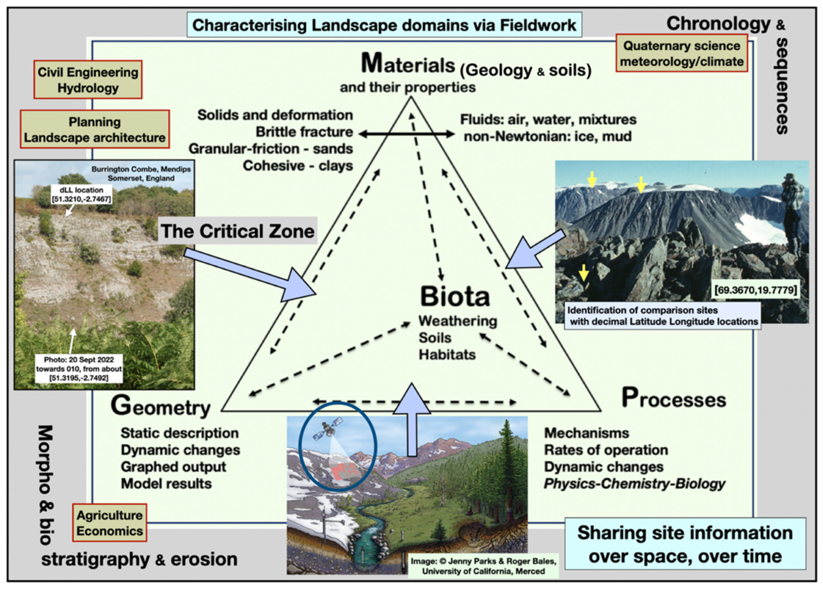
2.3. The Critical Zone

The Critical Zone (CZ) is a simple concept: the environment where rock, soil, water, air, and living organisms interact with and shape the Earth’s surface. As such, it encompasses the Earth sciences, especially geology, geomorphology and soil science as well as biological sciences and meteorology. Landslides and floods, vegetation and forestry are all in the domain of Critical Zone Science (CZS). Human interventions, especially in terms of environmental and climate change, are intimately linked via, for example, agriculture, productivity and soil erosion. Some of these interactions are shown in Figure 1 and presented in [8]. Critical Zone Observatories (CZOs) have been set up in various parts of the world akin to the Hubbard Brook Experimental Catchment used for a wide variety of ecological studies. Remote sensing techniques have been used for expanding knowledge about the local environment, for example [9]. More generally for CZOs, [10] show the French network and the importance of studying environmental, topographic, lithological as well as climatic gradients. The subsequent mention of mass movements, including slopes and rock glaciers, are all part of the CZ and are particularly susceptible to changes in the water balance in heating climates.

As Brantley et al. [11] indicate, ‘Conceptualizing the complex interplay of chemistry, biology, geology, and physics within the skin of the Earth as a system—the Critical Zone—forces scientists to work together across disciplines and scales. In so doing, scientists will learn how to interpret recurrent patterns observed in the CZ and how to protect the CZ for all life’. Using [dLL] is thus a way to explore the CZ and to incorporate shared findings in the Digital Earth. Banwart et al. [12] emphasized the significance of the CZ with reference to soils and weathering in a geochemical context:

Through unsustainable land use practices, mining, deforestation, urbanization, and degradation by industrial pollution, soil losses are now hypothesized to be much faster (100 times or more) than soil formation.

This is elaborated upon by Brantley et al. [11] and Banwart et al. ([12], p. 986):

We contend that the CZO approach is an essential advance in geoscience research and that the anticipated step change is urgently required. This is precisely because of the human pressure on the near-term habitability of Earth’s Critical Zone and the immense rate of ongoing environmental change.

As indicated in Figure 1, remote sensing plays an important part of such diverse studies in the CZ and the signals received and interpreted will be necessarily complex in space and time with results being reported in a wide variety of journals. This requirement shows the importance of the FAIR data principles, especially findability and inter-operability. Giardino and Houser [8] give examples of Earth surface processes, geomorphological, investigations associated with the CZ and, in [13] ‘Geospatial science and technology for understanding the complexities of the Critical Zone’ present some of the issues incorporated into Figure 1. The volume also provides an overview of CZOs [14] who mention monitoring ‘locations’ of CZOs in the USA. Although detailed data from CZOs are given, there are no notional geolocated links between them; they exist as separate environmental ’probes’, not as part of an information space as in the Digital Earth.

Observations have locations in space and time, illustrated by Brantley et al. [11] who show the importance of nodes at the junctions of environmental gradients. Maps may include the positions of stream gauges and water samplers, soil moisture sensors, etc. in specific watersheds but these locations are only named, not geolocated. Thus, there is no easy way to exchange and interchange data produced from sensors, whether remote or terrestrial. Not only does this lack interoperability of site location data, but there is no easy way to access these data for future work that might incorporate new ideas, techniques or sensor capabilities. A solution to this problem, achieving data according to the FAIR data principles, is discussed below. Using data at (or about) geolocations allows an ‘information landscape’ to be built up over time. Nodes, such as a [dLL] and vertices (edges) can be constructed with this information to build knowledge graphs [15].

In the following sections I suggest ways in which geolocation can be used for adding information to a variety of Earth surface features to develop information landscapes in the Digital Earth and the Critical Zone. I concentrate on the data and information reported by remote sensing techniques rather than the techniques themselves.

3. Considerations of Geolocation in Remote Sensing Applications

3.1. Landslides, Elevation Models and Geomorphic Identity

A recent example of climate control on landsliding in the eastern Pamirs is given by Pei et al. [16]. No geo-located data points are provided, so it is difficult to see the significance of data outliers from fitted regressions. The ‘overview of the landslide sites visited’ ([16], Figure 6) shows the types and ‘triggering factors’ of landslides but not their geolocations. The images used are a mix of terrestrial field site photos and Google Earth, but it is not easy to examine the landslide locations independently via GE. This is unfortunate as a paper on rock glacier mapping [17] from a similar arid area (western Kunlun Shan) indicates a debris flow planform as a ‘rock glacier type’ used as part of a machine learning mapping project. The feature, [35.708, 80.803], has been independently (unpublished) assessed as a mud/debris slide and appears very similar to several examples in [16]. Improved geo-location and the use of GE to provide ground truth in context, rather than outlines devised to test ML algorithms, would be helpful in the elucidation of landforms in their climatic context. The simple expedient is to include [dLL] geolocations as metadata for images, maps and other data sources.

Similarly, metadata and data points in tables, lists and inventories should be included as a matter of course. Shape and GeoTIFF files from GIS analyses alone are insufficient for FAIR data and should be supplemented by basic [dLL] located data as csv files. These data should preferably be as supplementary material for published papers with their own DOI.

The AGU ‘Landslides Blog’ [18] includes DD, but not yet full [dLL] identification, for many recent geomorphological events recorded as still and video images. In general, geotechnical and engineering geological mapping can be enhanced through use of [dLL] locations and enhance the data used in publications, reports and theses.

Earth Observation (EO) techniques have long been used to investigate landslide mapping. For example, [19] used Interferometric Synthetic Aperture Radar (InSAR) and Object-Based Image Analysis (OBIA) to investigate several sites in different geological settings for emergency management and mitigation purposes. The aim, as elsewhere in such studies, is to produce a local map rather than provide any integration into DE. Digital Elevation Models, DEM, are useful for many purposes and are an important precondition for many applications. They are particularly significant in regions that are devoid of detailed topographic maps. Forkuor and Maathuis [20] compare DEMs and Fleming et al. [21] (2010) note that, ’elevation data are a critical element in most geoscience applications’. DEMs have been found useful in many fields of study, such as geomorphometry, being primarily related to surface processes such as landslides that can be identified in a DEM. For example, Fleming et al. [21] compared results from Shuttle Radar Topographic Mission (SRTM) and ASTER-derived DEMs for hydrological and environmental modelling. Other comparisons, with more recent sensors, can be compared via DEMs. The publicly available ArcticDEM Digital Surface Models have been used for investigating dimension changes of glaciers [22] and slope-soil conditions related to aspects of local slope and groundwater conditions [23]. Pelletier [24] presents many examples of quantitative modelling of Earth surface processes that require links between materials and processes (MPGB in Figure 1), elevation models and remotely sensed data. These are individual case studies, and it would be helpful to be able to link, for example, local conditions to changing global conditions. A review of data from studies addressing climate-related dynamics of various form of slope failures (mass movements) in the European Alps [25] provides an important overview of papers. However, there is no compilation of data such that digital searches using geolocations might reveal. Similarly, the production of landslide susceptibility maps [26] involves the use of LiDAR, DEMs and fuzzy logic but does not reconcile site complexities that involve material properties (Figure 1) together with slope geometries. Using [dLL] for detailed site analysis and data recording aids such endeavors to monitor changes, especially those of a catastrophic nature, in the Critical Zone. Georeferencing in this manner also allows point-of interest (POI) techniques in social networks [27] to be linked to land surface features and other attributes germane to the CZ, especially for management purposes.

3.2. Information Aggregation in Information Landscapes

Information can be associated with an ‘object’ in various ways, and we are very familiar with this concept. A photograph taken on a mobile (cellular) phone is an obvious object and image recognition and classification can now be commonly used in mobile apps. Adding geolocation explicitly allows other questions to be asked in a variety of new ways.

A photograph of a bird can be imported into an app and identified against a suitable training set of images or songs. Traditionally, an appropriate bird field guide is used, and binomial classifications allow an easy way of differentiating between a North American robin (Turdus migratorius) and the European robin (Erithacus rubecula) and the various Australian ‘robins’ of the family Petroicidae, which may appear similar as in ‘robin red breast’. The binomial may also provide other information, such as conservation status. Changing metadata may be found, such that Wikipedia, outlines the re-classification of Erithacus rubecula from the thrushes to Old Word Flycatcher family; (Muscicapoidae, Fleming J, 1822). Here, Fleming, refers to John Fleming (1785–1857) the naturalist whose grave lies in Dean Cemetery in Edinburgh [55.952, −3.222] and is also named for Fleming Fjord in E Greenland [71.737, −22.804]. The geologist-glaciologist James David Forbes (1809–1868), who invented one of the first modern seismometers, is also buried in Dean Cemetery. A book on the glaciological work of J.D. Forbes has been compiled by Cunningham [28]. We might bring together some of this information in a short-form data set such as; {Dean Cemetery [55.952, −3.222], James David, John Fleming, Edward Forbes}. Various name/data investigations can obviously be followed from this basic information held as a simple knowledge graph. We can also explore information associated with a specific location as well as names. Notice that the [dLL] is a unique identifier for a place. It differs from a place label, usually a toponym but here, Dean Cemetery, is an area where numerous people have memorials and whose locations can be identified on the ground. A dataset can be produced locally for a specific use, such as a graveyard map. The ‘Overpass API’ (formerly Open Street Map Server Side Scripting) can be used to access information and the uMap facility allows a variety of information stories to be produced. Essentially, these are linked via [dLL] so an information surface, as a local map of the cemetery, might be made allowing various ways to cross-identify memorial locations, named people, their achievements etc. to produce a geolocated ‘information landscape’. Such data sets ‘chunk’ information, digital and textual.

3.3. Entities in Landscapes

If we take a [dLL]-specified unit (whether it be landform, monument or sampling point) then we can consider it to be unique example of a ‘natural kind’, a unit that is an intellectual grouping, or categorization of things, in a manner that is reflective of the actual world. An example is ‘car’ = ‘automobile’, depending on the type of ‘English’, a more difficult example is ‘chair’—which, although it/they can be recognized visually, is surprisingly difficult to define [29]. This difficulty is also the case for many landforms. We can designate a coding for a mountain summit as SU and add its location to a name or names, thus; {Mount Everest, Chomolungma/Qomolangma, Sagarmatha SU [27.9881,86.9251]}. Mapping the entities SU higher than 8 000 m can be done easily. Mapping the glaciers that descend from summits is less easy but has been done via GLIMS (Global Land Ice Measurement from Space) [30] and their changing boundaries over time in the Randolph Glacier Inventory (RGI). The limits of glaciers (digraph coding GL) are not always easy to define, however, as albedo changes, where debris accretes on glacier surfaces to become ‘debris covered glaciers’ (GLd), with variable fuzzy edges. Amongst others, King et al. [31] have used remote sensing to determine selected glacier surface profiles and debris cover evolution, while Jones et al. [32] produced an inventory of some 6000 rock glaciers (RG) in the Nepalese Himalaya. Rock glaciers have hydrological significance [32] as well as glaciers, so their identification and mapping are clearly important with respect to many mountain domains in the Digital Earth, not just the Himalaya. However, GLIMS and the RGI generally do not include RG in their catalogues, even though debris covered glaciers are associated with them [33].

There are groupings in physical geography which, unlike landforms, refer to properties that are not easily identifiable by remote sensing. Periglacial, a rather nebulous term, and ‘permafrost’, a ground temperature condition, are two areal concepts that cannot, unlike ‘glacier’, be mapped easily. The term ‘mountain domain’ (𝔻𝕞), analogous to coastal domain, is used as a general term in which specific landforms, such as SU, GL and RG (and many others), can be identified and mapped [34]—unlike periglacial and permafrost. In brief, the problem is what do RG signify? Are RG all similar in morphology and origin and how do they relate to glaciers, debris covered glaciers (GLd) and relict snowbanks in landscapes that are losing ice mass? The literature usually quoted in remote sensing journals tends to follow a geographical, zonal climate, approach as promulgated by Barsch [35], that all RG denote permafrost in the mountains. However, ground truth investigations beyond simple remote sensing recognition of landform morphology show that RG entities are closely coupled with both debris and ice supplies derived from and via other landforms.

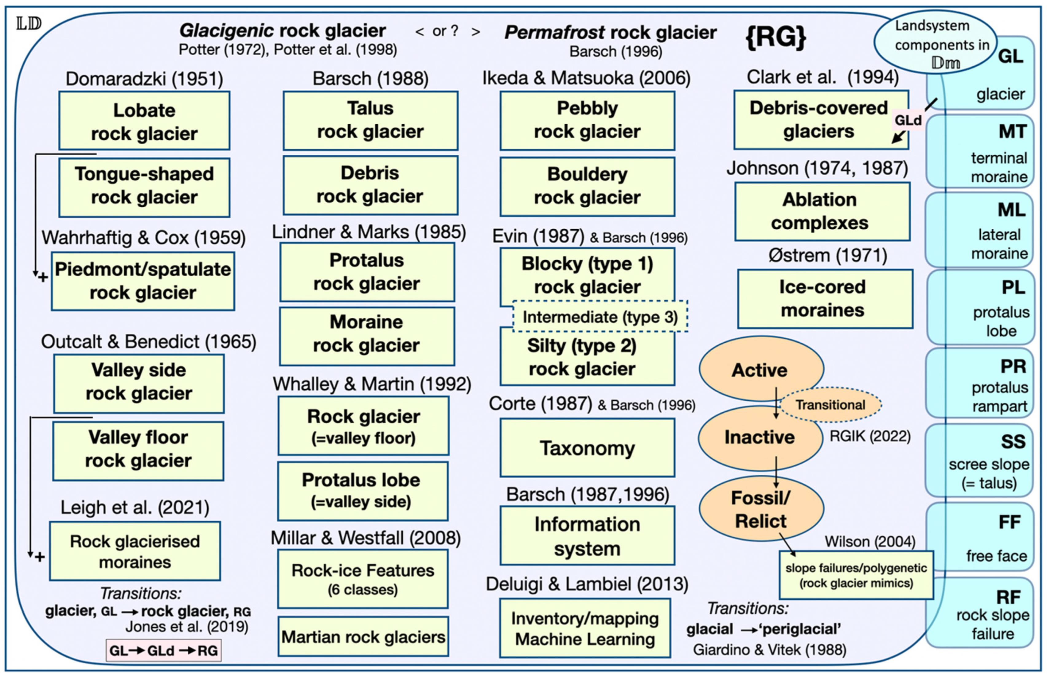
3.4. Rock Glaciers and [dLL] Geolocation

In recent years the distinctive mountain landforms, ‘rock glaciers’ (RG) have become of interest beyond geomorphology. For the remote sensing community, they have been used as a landform to test techniques. For example, the inventory of RG in the Sierra Nevada of California [36] was mainly from field observations and supplemented by aerial photography. The study by Liu et al. [37] of surface motion of selected RG in the area, used InSAR to determine surface velocities as a complement to optical imaging. Other studies, again associated with various inventories [38,39,40]. Machine learning for mapping purposes has been used in the mountain domain (𝔻𝕞) such as for glaciers (GL) [41] and debris covered glaciers (GLd, which are related to RG and GL) [42], glacier recession [43] and landslide susceptibility [44]. Surface activity and movement of RG have also been studied [45,46]. Permafrost mapping and modelling using SRTN imagery has been reported [47] assuming that RG indicate the ground thermal condition of mountain permafrost. Such papers raise interesting problems for the geomorphologist in elucidating these complex features. Many papers present new data from remote sensing, but the following questions—which relate specifically to remotely sensed data and their interpretation—need to be linked to Materials–Processes–Geometry geomorphological investigations in the Critical Zone (Figure 1). Thus, various questions arise:

• What is an RG and how does it, or does not, relate to GL and GLd?
• What do RG signify environmentally and geomorphologically? The key question, are they permafrost or glacier ice bodies?
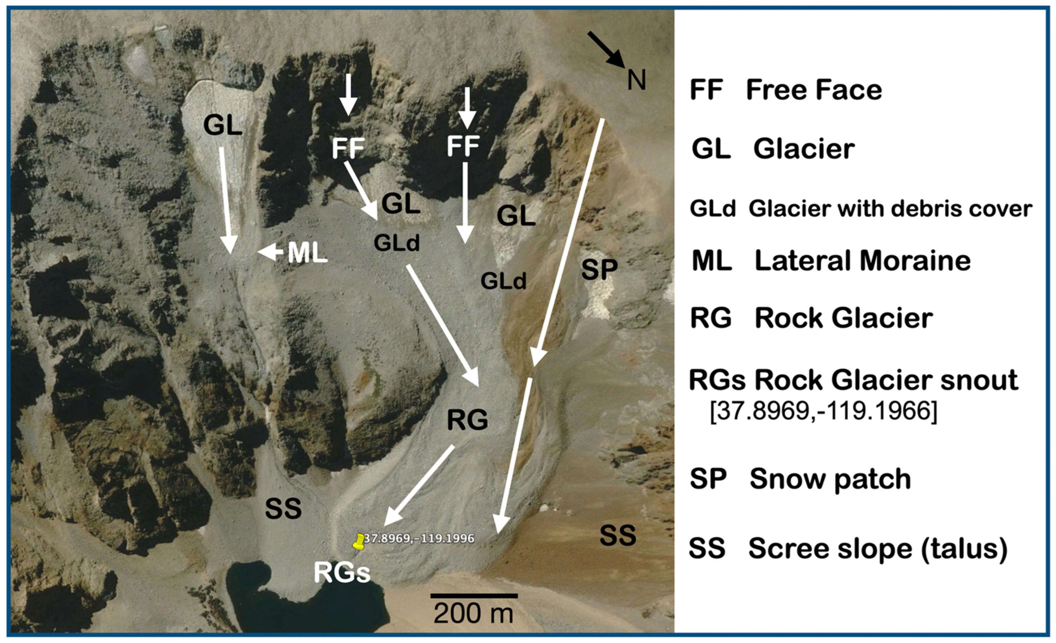
• How are RG distinguished on the Earth’s surface and can they be differentiated from glaciers, GL?
• How can RG, GL and GLd be used in inventories, e.g., to determine water content or extent of permafrost?

These are questions that are still being debated in the geomorphological community and cannot be answered fully here. However, I now suggest possible responses (if not answers) to these queries using case studies identified by [dLL] as ’ground truth’ locations. I also point out some misapprehensions and cautions in the use of definitions, but note that some difficulties can be ameliorated if all sites are geolocated via the common [dLL] geolocation format.

Rock glaciers are:

Found on slopes, a mass of rock fragments and finer material that contains either interstitial ice or an ice core and shows evidence of past or present movement

COMMEMT: rock glaciers do not form if there is insufficient moisture to form the interstitial ice that permits movement of the mass. Some are believed to have been formed, at least partly, by burial of glacier ice. Active tock glaciers move at speeds up to 50 m per year * and possess a steep front with slope angles greater than the angle of repose. Rock glaciers are said to be inactive when the main body ceases to move. Most rock glaciers have transverse ridges and furrows on their surface (National Research Council Canada, 1988 ([48], p. 75).

* Most authorities, such as Washburn ([49], Table 6.4) indicate <1 m/year; the 50 m per year is probably a misprint for cm per year.

Point 1. Perhaps the easiest way to show what a rock glacier ‘is’ can be achieved by showing a photograph (Figure 2) with a location that has been used elsewhere [37]. The possible relationship to other features, such as debris supply to glaciers, rock glaciers and scree slopes from the disintegration of cliffs (free faces, denoted by FF).

Point 2. There is a long-standing discussion about what RG signify and the following is only a brief outline of problems with the ‘RG indicate permafrost’ model. The definition cited above relates to both interstitial ice and permafrost (ground ice) but also, ’by burial of glacier ice’. The discussion and classification of Millar and Westfall [36] includes RG that ‘appear to derive from ice glaciers; and others yet appear to originate from cumulative snow-, ice- and rockfall events’. However, there is a widely held view that rock glaciers are only the result of ‘permafrost creep’ [51] and particularly that, ‘only the ice-cemented rock glacier seems acceptable in our present state of knowledge. It contains ice, often more than 50 percent of its volume, but this ice is permafrost ice. Large bodies of glacier ice have not yet been encountered in a true rock glacier’ [52]. This ‘permafrost only’ interpretation has led to the notion that rock glaciers can be used to help map permafrost in mountains, such that rock glacier inventories can be used for mapping (Point 4), ‘Permafrost presence or absence can be derived from rock glacier maps, based on their activity. Indeed, active or inactive rock glaciers suggest the existence of permafrost conditions, whereas relict ones indicate its absence’ ([53], p. 371). The RG as ‘permafrost only’ indicators is not only dependent upon statements as in the foregoing, but is associated with the notions (dating from 50–100 years ago) that areas deemed ‘periglacial’ do not include glaciers. When looking at a mountain domain this makes little sense when glaciers are clearly part of the scene overall. This scenario also applies to ‘permafrost’ in the mountains. To provide a general view in a landscape that includes glaciers, or their previous presence as noted by moraines, we consider all landforms in a landscape. Each entity can be uniquely identified, and compared, via [dLL] as in Figure 2. Landsystems may incorporate a variety of landform entities giving a similar overall appearance despite each entity being unique.

Point 3. RG are essentially recognized by their overall topography, as in the description/definition noted previously and seen in Figure 2. This is a ‘tongue-shaped’ rock glacier. However, there are other related landforms, some of which are noted in Figure 3. Hence a ‘landsystem’ approach encompasses a wide variety of landforms that may grade into each other. Some of these are seen in Figure 3, together with some of the classifications and typologies associated with RG. All these landforms sit within the landscape domain (𝕃𝔻) which includes the mountain environment, 𝔻𝕞, an example of which is in Figure 2. This holistic approach allows other landscapes to be discussed and brought together (Figure 1).

Point 4. Many recent papers using remote sensing techniques have produced ‘inventories’. Some papers have looked at operator variability [76] whilst others [77] have used InSAR kinematics to compare inventories using a moving area technique. As with many other recent papers, examples allow comparison of landforms. Sometimes these forms are given co-ordinates (e.g., as dms [77]) but some images have no geolocation. Some comparisons are cross-kinematics (velocity variability), some cross typologies (Figure 3) and some use other typologies, e.g., relict/intact forms [78] and a mixture of types [79] genesis and shape but with no geolocation of any kind. The work of Abdullah et al. [80] mixes a variety of RG classifications (Figure 3), such as by shape and activity and again the examples shown by them are not geolocated. This lack of geolocation is detrimental to interpretations and future use of published data.

There are clearly much valuable data, derived from remote sensors, contained in these papers and the resultant inventories. However, a lack of common geolocation restricts their widespread usage to allow data sharing and investigate combinations of landforms and environments. Moreover, inventories are only lists and not catalogues (such as astronomers use star catalogues). The [dLL] format would provide uniformity of identification and classification in a manner that is not yet possible. The complexities of RG classifications and typologies (Figure 3) reflect the variables interacting. Furthermore, where data analyses are presented from inventories, there is a tendency to produce aggregated results; means, box–whisker plots [81], violin plots of aspect angle [38,82]. Where bivariate plots are sometimes used; Kaldybayev et al. [38] plot distribution of the ‘kinematic activity’ of RG is by height. Although many data points are shown, each presumably geolocated, the only conclusion stated [38] is that ‘The highest surface velocity was found at altitudes of 3000–3400 m ASL (Figure 13). Most likely, this is due to the fact that 68% of the total area of the inventoried rock glaciers is located in this interval’. Although this is a ‘true’ statement, its information content is low and results from using bivariate data and not multivariate and georeferenced data. Many multivariate methods could be used, especially if analyses were to investigate differences (or similarities) between mapped features held in proper databases, rather than in lists. Catalogue databases could then be used to explore data relationships, such as by knowledge graphs.

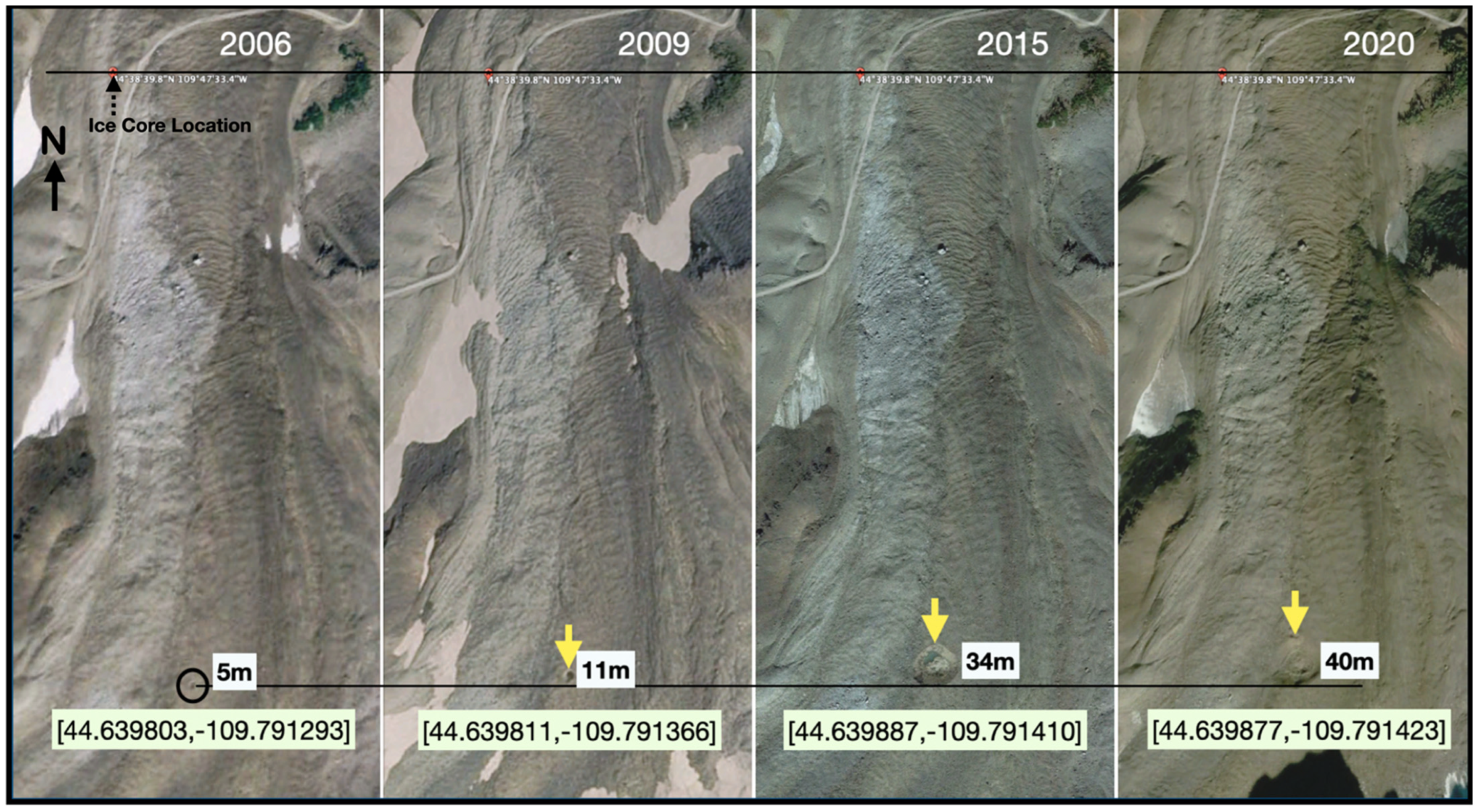
3.5. Identification of Glacier Ice-Cored Rock Glaciers

The RGIK methodology [71] invites RG activity, whether they are moving or not, to be assessed, preferably by measurement of movement and explicitly using InSAR. The approach also suggests geomorphological investigations. As with many of the papers cited earlier, for example Bertone et al. [77], the permafrost model is invoked specifically [70]. As mentioned previously, ‘Rock glaciers are creeping masses of frozen debris in the mountain periglacial landscape. Morphologically, they are characterized by a distinct front, lateral margins, and often by ridge-and-furrow surface topography’.

Several papers have recently used GE to show the glacial nature of debris-buried glacier ice and the continuum of the material (and hence continuum mechanics), for example in the Hindu Kush [83]. I now show how simple GE examination can identify glacier ice cores and melt features in both GLd and RG. Further, that with improved resolution and more imagery available, simple pattern recognition techniques could show glacier melting and ice down-wasting by identifying specific landforms that are responding to environmental changes.

Figure 4 shows the development, by widening of a surface meltpool, in the surface of the Galena Creek RG [44.6503, −109.7908] studied by Potter [68]. Barsch [35] has argued that the evidence from this RG shows it not to be ‘glacier-derived’ but additionally ([35], p. 214), ‘The Galena Creek rockglacier has to be accepted as a (normal) multiunit rockglacier, which is probably more a talus rockglacier than a debris rockglacier. Therefore, the model of the so-called ice-cored rock glacier has to be abolished’. Field and remotely sensed data now show clear evidence to the contrary.

A summary dataset showing the published contrary, glacier-ice-cored RG can be stated in fully digital format {Galena Creek RG[44.6503, −109.7908](doi.org/10.1111/j.0435-3676.1998.00042.x)(doi.org/10.1111/j.0435-3676.1998.00044.x)(doi.org/10.1017/jog.2019.67)(doi.org/10.1111/j.0435-3676.1998.00041.x)(doi.org/10.1130/0016-7606(1972)83[3025:irggcn]2.0.co;2)(doi.org/10.1002/esp.5678)}. The last of these papers shows Noel Potter with a glacier ice core extracted on a field trip, disproving Barsch’s statements. Petersen et al. ([84], Figure 2) show a meltpool (sometimes called a thermokarst pond) as a ground truth location for a geophysical survey, indicating glacier ice below a thin surface debris layer (Figure 4). This aggregation of information includes images, geolocations and paper authorship as a ‘searchable bundle’ in a way similar to the example of memorials in Edinburgh’s Dean Cemetery.

The significance of meltwater pools and sub-debris glacier surface changes is directly related to the glacier’s response to global heating. Mountain landsystems in the Andes are particularly prone to the formation of these meltpools. Developing glacier-melt features (Figure 5) can be identified in GE as a glacier-rock glacier system in the Juncal Masssif, Chile–Argentina border. This GL–GLd–RG landsystem is in accord with the glacier hydrological investigations of Rodriguez et al. [85] in this area. Although each rock glacier system is unique in overall topographic shape and glacier and debris mass balances, the meltpools have similar recognizable features. Tracking them over time via [dLL] would be a good way to bring pattern recognition techniques from remote-sensing data to look at a very wide area, such as the whole of the Andes, to monitor climate change. As well as meltpool formation, surface elevation changes could also be monitored to produce maps of ice mass change accruing to, for example precipitation and temperature gradients in remote areas.

4. General Discussion

The contributions of remote sensing technologies to geomorphology in the mountain domain and the Critical Zone in general are undeniable. More data will accrue as remote sensing technology with specialist sensors contribute to enhanced optical and radar observations. Good ground truth data are required to test, train and build confidence in geological models [86]. Some data related to the complex topographical features known as rock glaciers have been presented in the previous section, not least the long-standing controversy concerning their nature and interpretation. Observations indicate that RG should not be considered as uniquely determined by the thermal conditions known as ‘permafrost’, but that glacier ice acts as a continuum substrate that can accumulate rock debris on its surface. These findings tend to negate many existing definitions of RG [48] and models need to be revised. The increasing debris thickness insulates the ice and, consequently, the glacier can still flow actively and extend downslope. Rock glacier behavior depends not so much on the thermal properties of ice as its rheological properties under low stresses (of surface slope and thickness). The interface between a melting glacier surface under a debris cover can be seen in meltwater pools. Google Earth, with its improved resolution over traditional aerial photography, can show the enlargement of these pools and movement over time. These observations, rarely indicated in large scale mapping, show the importance of ground truth. The use of explicit, [dLL], georeferencing of these locations conforms to the view that observations are made at locations and within time-frames. The easily accessed facilities in Google Earth provide data checking of both field and satellite imagery. Tagging images, of field sites for example, with [dLL] and other metadata, allows sites to be cross referenced. Such information can be grouped (or ‘chunked’) as an information tensor [49] with the [dLL] location as an index that can be used in a database. A database, a searchable bundle, could be built with [dLL] referencing to encompass all the inventories produced in a searchable, digital, catalogue. Multi-dimensional analytical methods are rarely used for analyzing rock glacier data. An exception is the discriminant analysis relating RG features to climate data [36].

One problem with the ‘permafrost’ model of rock glacier formation is that it does not take into account the downhill movement of ice and rock debris in the manner of its rheology [87,88]. The debris may cover the glacier component completely, or almost so (Figure 2), making it difficult to identify and delimit features by remote sensing methods. The glacier model involves the continuity of material transport. In Figure 2 this is from cliff top through components FF, SS and RG to RGs. Sometimes the, very small, glacier component may not be easily visible and may disappear over time as in Figure 2. I suggest that new methods be developed that take these ‘contributing areas’ into account, perhaps with fuzzy boundaries that may change over time. Overlaying images onto digital elevation models, together with data about velocity changes, allow kinematic (and dynamic, with forces on materials) information to be mapped into the Digital Earth. Testing such methods and algorithms on slow-moving landsystems such as rock glaciers may eventually allow faster-moving events in the Critical Zone (Figure 1) to be tracked in near real-time. Examples might include flooding events, landsliding produced by a progressing storm track or assessing forest fire paths. Using [dLL] would make these developments easier to implement.

5. Conclusions

Remotely sensed data are important in identifying complex features in the Critical Zone. Rock glaciers, RG, have been used as an important geomorphological feature, now widely referenced in the environmental literature, that can be investigated with the attribution of [dLL] geolocation. The full scientific usefulness of RG and their interpretation has, however, been held back by a dated, and scientifically disproven notion, that of the ‘permafrost rock glacier’.

The importance of using a precise geolocator to identify points with associated information, such as for RG, has been demonstrated. Geolocating via [dLL] allows open results to be presented on FAIR data principles, specifically that RG are part of a glacier-debris accumulation landsystem and not the result of the presence of permafrost. Thus, RG cannot be used to map the presence of permafrost in the mountain domain.

The main conclusions can be listed:

• The use of a uniformly recognized geolocation formal, [dLL], allows unique locations on the surface of the Earth to be identified and shared. It thus has an important part to play within the FAIR data usage doctrine.
• [dLL] can be used in image metadata to identify any object or feature as well as the vantage point of a field photograph.
• [dLL] can be used to identify a feature that might require repeated survey, perhaps over an appropriate time interval to ascertain change, e.g., vegetation. This might be a satellite sensor, ground control site or part of a UAV survey (Figure 1).
• A transect can be determined by a [dLL] as origin (Figure 2). This transect contains information (an information tensor) that can be linked to a resurvey or analysis with a new sensor. Transects, as with point locations, can be test sites for providing model checking or ground truth.
• [dLL] can provide the important links in data sets; [dLL]{other information, web sites etc, dates} as a searchable bundle in digital form. This is especially important when [dLL] are used as database reference objects or identifiers.
• Using [dLL] as datapoints allows data to be linked as nodes in knowledge graphs for visualization and analysis or in a GIS.
• Publications should enhance the FAIR data principles by using [dLL] in image metadata, data tables. The basic data set, including [dLL], should be included within the paper in a simple csv file to ensure compatibility with other investigations.

These findings indicate that data usage, associated with [dLL], maximize its cost-effectiveness when used in studies involving remotely sensed data. As data have both position and time, it is beneficial for future research to include these, as appropriate, in future work relating to Earth surface geolocation.

References

1. Aswathi, J.; Kumar, R.B.; Oommen, T.; Bouali, E.; Sajinkumar, K. InSAR as a tool for monitoring hydropower projects: A review. Energy Geosci. 2022, 3, 160–171. [Google Scholar] [CrossRef]
2. Zwieback, S.; Liu, L.; Rouyet, L.; Short, N.; Strozzi, T. Advances in InSAR Analysis of Permafrost Terrain. Permafr. Periglac. Process. 2024, 1–13. [Google Scholar] [CrossRef]
3. Whalley, W.B. Landscape Domains and Information Surfaces: Data Collection, Recording and Citation Using Decimal Latitude-Longitude Geolocation via the FAIR Principles. Earth Surf. Process. Landf. 2023, 48, 11. [Google Scholar] [CrossRef]
4. International Symposium on Digital Earth. International Symposium on Digital Earth. International Symposium on Digital Earth–Digital Earth in Action. In Center for Earth Observation and Digital Earth; Chinese Academy of Sciences: Beijing, China, 2009; Available online: https://web.archive.org/web/20120227195943/http:/159.226.224.4/isde6en/hykx11.html (accessed on 10 June 2024).
5. Whalley, W.B. Enhancing the Digital Earth via Digital Decimal Geolocation and the FAIR Data Principles. Earth Sci. Syst. Soc. 2024, 10110. [Google Scholar] [CrossRef]
6. Gabrielli, S.; Spagnolo, M.; De Siena, L. Geomorphology and surface geology of Mount St. Helens Volcano. J. Maps 2020, 16, 585–594. [Google Scholar] [CrossRef]
7. Sobolewski, L.; Hansteen, T.H.; Zorn, E.U.; Stenner, C.; Florea, L.J.; Burgess, S.A.; Ionescu, A.; Cartaya, E.; Pflitsch, A. The evolving volcano-ice interactions of Crater Glacier, Mount St. Helens, Washington (USA). Bull. Volcanol. 2023, 85, 22. [Google Scholar] [CrossRef]
8. Giardino, J.R.; Houser, C. Principles and Dynamics of the Critical Zone; Elsevier: Amsterdam, The Netherlands, 2015. [Google Scholar]
9. Diao, C. Complex network-based time series remote sensing model in monitoring the fall foliage transition date for peak coloration. Remote Sens. Environ. 2019, 229, 179–192. [Google Scholar] [CrossRef]
10. Gaillardet, J.; Braud, I.; Gandois, L.; Probst, A.; Probst, J.-L.; Sanchez-Pérez, J.M.; Simeoni-Sauvage, S. OZCAR: The French network of critical zone observatories. Vadose Zone J. 2018, 17, 1–24. [Google Scholar] [CrossRef]
11. Brantley, S.L.; Goldhaber, M.B.; Ragnarsdottir, K.V. Crossing disciplines and scales to understand the critical zone. Elements 2007, 3, 307–314. [Google Scholar] [CrossRef]
12. Banwart, S.; Bernasconi, S.M.; Bloem, J.; Blum, W.; Brandao, M.; Brantley, S.; Chabaux, F.; Duffy, C.; Kram, P.; Lair, G. Soil processes and functions in critical zone observatories: Hypotheses and experimental design. Vadose Zone J. 2011, 10, 974–987. [Google Scholar] [CrossRef]
13. Bishop, M.P.; Dobreva, I.B.; Houser, C. Geospatial Science and Technology for Understanding the Complexities of the Critical Zone. In Developments in Earth Surface Processes; Elsevier: Amsterdam, The Netherlands, 2015; pp. 523–561. [Google Scholar]
14. White, T.; Brantley, S.; Banwart, S.; Chorover, J.; Dietrich, W.; Derry, L.; Lohse, K.; Anderson, S.; Aufdendkampe, A.; Bales, R. The Role of Critical Zone Observatories in Critical Zone Science. In Developments in Earth Surface Processes; Elsevier: Amsterdam, The Netherlands, 2015; pp. 15–78. [Google Scholar]
15. Barrasa, J.; Webber, J. Building Knowledge Graphs. In A Practitioner’s Guide; O’Reilly: Sebastopol, CA, USA, 2023. [Google Scholar]
16. Pei, Y.; Qiu, H.; Zhu, Y.; Wang, J.; Yang, D.; Tang, B.; Wang, F.; Cao, M. Elevation dependence of landslide activity induced by climate change in the eastern Pamirs. Landslides 2023, 20, 1115–1133. [Google Scholar] [CrossRef]
17. Hu, Y.; Liu, L.; Huang, L.; Zhao, L.; Wu, T.; Wang, X.; Cai, J. Mapping and Characterizing Rock Glaciers in the Arid West Kunlun Mountains Supported by InSAR and DeepLearning. J. Geophys. Res. Earth Sci. 2023, 128, e2023JF007206. [Google Scholar] [CrossRef]
18. Petley, D. The Landslide Blog. Available online: https://blogs.agu.org/landslideblog/ (accessed on 5 September 2023).
19. Casagli, N.; Cigna, F.; Bianchini, S.; Hölbling, D.; Füreder, P.; Righini, G.; Del Conte, S.; Friedl, B.; Schneiderbauer, S.; Iasio, C. Landslide mapping and monitoring by using radar and optical remote sensing: Examples from the EC-FP7 project SAFER. Remote Sens. Appl. Soc. Environ. 2016, 4, 92–108. [Google Scholar] [CrossRef]
20. Forkuor, G.; Maathuis, B. Comparison of SRTM and ASTER derived digital elevation models over two regions in Ghana-Implications for hydrological and environmental modeling. In Studies on Environmental and Applied Geomorphology; Piacentini, T., Miccadei, E., Eds.; INTECH: Rijeka, Yugoslavia, 2012. [Google Scholar] [CrossRef]
21. Fleming, C.; Giles, J.; Marsh, S. Elevation Models for Geoscience; Special Publication 345; Geological Society of London: London, UK, 2010. [Google Scholar]
22. Barr, I.D.; Dokukin, M.D.; Kougkoulos, I.; Livingstone, S.J.; Lovell, H.; Małecki, J.; Muraviev, A.Y. Using ArcticDEM to analyse the dimensions and dynamics of debris-covered glaciers in Kamchatka, Russia. Geosciences 2018, 8, 216. [Google Scholar] [CrossRef]
23. Atkinson, J.; de Clercq, W.; Rozanov, A. Multi-resolution soil-landscape characterisation in KwaZulu Natal: Using geomorphons to classify local soilscapes for improved digital geomorphological modelling. Geoderma Reg. 2020, 22, e00291. [Google Scholar] [CrossRef]
24. Pelletier, J. Quantitative Modeling of Earth Surface Processes; Cambridge University Press: Cambridge, UK, 2008. [Google Scholar]
25. Jacquemart, M.; Weber, S.; Chiarle, M.; Chmiel, M.; Cicoira, A.; Corona, C.; Eckert, N.; Gaume, J.; Giacona, F.; Hirschberg, J. Detecting the impact of climate change on alpine mass movements in observational records from the European Alps. Earth-Sci. Rev. 2024, 104886. [Google Scholar] [CrossRef]
26. Okoli, J.; Nahazanan, H.; Nahas, F.; Kalantar, B.; Shafri, H.Z.M.; Khuzaimah, Z. High-Resolution Lidar-Derived DEM for Landslide Susceptibility Assessment Using AHP and Fuzzy Logic in Serdang, Malaysia. Geosciences 2023, 13, 34. [Google Scholar] [CrossRef]
27. Li, Z.; Cheng, W.; Xiao, H.; Yu, W.; Chen, H.; Wang, W. You are what and where you are: Graph enhanced attention network for explainable poi recommendation. In Proceedings of the 30th ACM International Conference on Information & Knowledge Management, 2021, Gold Coast, QLD, Australia, 1–5 November 2021; pp. 3945–3954. [Google Scholar] [CrossRef]
28. Cunningham, F. James David Forbes, Pioneer Scottish Glaciologist; Scottish Academic Press: Edinburgh, UK, 1990. [Google Scholar]
29. Grabner, H.; Gall, J.; Van Gool, L. What makes a chair a chair? In Proceedings of the Confderence on Computer Vision and Pattern Recognition 2011, Colorado Springs, CO, USA, 20–25 June 2011; pp. 1529–1536. [Google Scholar] [CrossRef]
30. Raup, B.; Racoviteanu, A.; Khalsa, S.J.S.; Helm, C.; Armstrong, R.; Arnaud, Y. The GLIMS geospatial glacier database: A new tool for studying glacier change. Glob. Planet. Chang. 2006, 56, 101–110. [Google Scholar] [CrossRef]
31. King, O.; Turner, A.G.; Quincey, D.J.; Carrivick, J.L. Morphometric evolution of Everest region debris-covered glaciers. Geomorphology 2020, 371, 107422. [Google Scholar] [CrossRef]
32. Jones, D.B.; Harrison, S.; Anderson, K.; Shannon, S.; Betts, R. Rock glaciers represent hidden water stores in the Himalaya. Sci. Total Environ. 2021, 793, 145368. [Google Scholar] [CrossRef]
33. Jones, D.B.; Harrison, S.; Anderson, K.; Whalley, W.B. Rock glaciers and mountain hydrology: A review. Earth-Sci. Rev. 2019, 193, 66–90. [Google Scholar] [CrossRef]
34. Whalley, W.B. The glacier-rock glacier mountain landsystem: An example from North Iceland. Geogr. Ann. A 2021, 103, 1–22. [Google Scholar] [CrossRef]
35. Barsch, D. Rockglaciers. In Indicators for the Present and Former Geoecology in High Mountain Environments; Springer: Berlin/Heidelberg, Germany, 1996; p. 331. [Google Scholar] [CrossRef]
36. Millar, C.I.; Westfall, R.D. Rock glaciers and related periglacial landforms in the Sierra Nevada, CA, USA; inventory, distribution and climatic relationships. Quat. Int. 2008, 188, 90–104. [Google Scholar] [CrossRef]
37. Liu, L.; Millar, C.I.; Westfall, R.D.; Zebker, H.A. Surface motion of active rock glaciers in the Sierra Nevada, California, USA: Inventory and a case study using InSAR. Cryosphere 2013, 7, 1109–1119. [Google Scholar] [CrossRef]
38. Kaldybayev, A.; Sydyk, N.; Yelisseyeva, A.; Merekeyev, A.; Nurakynov, S.; Zulpykharov, K.; Issanova, G.; Chen, Y. The First Inventory of Rock Glaciers in the Zhetysu Alatau: The Aksu and Lepsy River Basins. Remote Sens. 2023, 15, 197. [Google Scholar] [CrossRef]
39. Ma, Q.; Oguchi, T. Rock Glacier Inventory of the Southwestern Pamirs Supported by InSAR Kinematics. Remote Sens. 2024, 16, 1185. [Google Scholar] [CrossRef]
40. Villarroel, C.D.; Tamburini Beliveau, G.; Forte, A.P.; Monserrat, O.; Morvillo, M. DInSAR for a Regional inventory of active rock glaciers in the dry andes mountains of argentina and chile with sentinel-1 data. Remote Sens. 2018, 10, 1588. [Google Scholar] [CrossRef]
41. Zhang, J.; Jia, L.; Menenti, M.; Hu, G. Glacier facies mapping using a machine-learning algorithm: The Parlung Zangbo Basin case study. Remote Sens. 2019, 11, 452. [Google Scholar] [CrossRef]
42. Lu, Y.; Zhang, Z.; Shangguan, D.; Yang, J. Novel machine learning method integrating ensemble learning and deep learning for mapping debris-covered glaciers. Remote Sens. 2021, 13, 2595. [Google Scholar] [CrossRef]
43. Ganyushkin, D.; Chistyakov, K.; Derkach, E.; Bantcev, D.; Kunaeva, E.; Terekhov, A.; Rasputina, V. Glacier Recession in the Altai Mountains after the LIA Maximum. Remote Sens. 2022, 14, 1508. [Google Scholar] [CrossRef]
44. Lizama, E.; Morales, B.; Somos-Valenzuela, M.; Chen, N.; Liu, M. Understanding landslide susceptibility in Northern Chilean Patagonia: A basin-scale study using machine learning and field data. Remote Sens. 2022, 14, 907. [Google Scholar] [CrossRef]
45. Bertone, A.; Zucca, F.; Marin, C.; Notarnicola, C.; Cuozzo, G.; Krainer, K.; Mair, V.; Riccardi, P.; Callegari, M.; Seppi, R. An unsupervised method to detect rock glacier activity by using Sentinel-1 SAR interferometric coherence: A regional-scale study in the Eastern European Alps. Remote Sens. 2019, 11, 1711. [Google Scholar] [CrossRef]
46. Meng, T.M.; Aguilar, R.; Christoffersen, M.S.; Petersen, E.I.; Larsen, C.F.; Levy, J.S.; Holt, J.W. Photogrammetric Monitoring of Rock Glacier Motion Using High-Resolution Cross-Platform Datasets: Formation Age Estimation and Modern Thinning Rates. Remote Sens. 2023, 15, 4779. [Google Scholar] [CrossRef]
47. Khan, M.A.R.; Singh, S.; Pandey, P.; Bhardwaj, A.; Ali, S.N.; Chaturvedi, V.; Ray, P.K.C. Modelling permafrost distribution in western himalaya using remote sensing and field observations. Remote Sens. 2021, 13, 4403. [Google Scholar] [CrossRef]
48. National Research Council of Canada (Ed.) Glossary of Permafrost and Related Ground-Ice Terms, Technical Memorandum 142; National Research Council of Canada: Ottawa, ON, Canada, 1988.
49. Washburn, A.L. Geocryology: A Survey of Periglacial Processes and Environments; Wiley: Chichester, UK, 1979. [Google Scholar]
50. Whalley, W.B. Mapping small glaciers, rock glaciers and related features in an age of retreating glaciers: Using decimal latitude-longitude locations and ‘geomorphic information tensors’. Geogr. Fis. E Din. Quat. 2021, 44, 55–67. [Google Scholar] [CrossRef]
51. Haeberli, W. Creep of Mountain Permafrost: Internal structure and flow of alpine rock glaciers. Mitteilungen der Versuchsanstalt für Wasserbau. Hydrol. Glaziologie 1985, 77, 142. [Google Scholar]
52. Barsch, D. The problem of ice-cored rock glacier. In Rock Glaciers; Giardono, J.R., Shroder, J.F., Vitek, J.D., Eds.; Allen and Unwin: London, UK, 1987; pp. 45–53. [Google Scholar]
53. Deluigi, N.; Lambiel, C.; Kanevski, M. Data-driven mapping of the potential mountain permafrost distribution. Sci. Total Environ. 2017, 590, 370–380. [Google Scholar] [CrossRef]
54. Barsch, D. Rockglaciers. In Advances in Periglacial Geomorphology; Clark, M.J., Ed.; Wiley: Chichester, UK, 1988; pp. 69–90. [Google Scholar]
55. Clark, D.H.; Clark, M.M.; Gillespie, A.R. Debris-covered glaciers in the Sierra Nevada, California, and their implications for snowline reconstructions. Quat. Res. 1994, 41, 139–153. [Google Scholar] [CrossRef]
56. Corte, A.E. Rock glacier taxonomy. In Rock Glaciers; Giardino, J.F., Jr., Shroder, J.F., Jr., Vitek, J.D., Eds.; Allen and Unwin: London, UK, 1987; pp. 27–39. [Google Scholar]
57. Deluigi, N.; Lambiel, C. PERMAL: A Machine Learning Approach for Alpine Permafrost Distribution Modeling. Jahrestagung der Schweiz. Geomorph. Ges. 2013. Available online: https://www.researchgate.net/publication/267393953_PERMAL_a_machine_learning_approach_for_alpine_permafrost_distribution_modeling (accessed on 10 June 2024).
58. Domaradzki, J. Blockströme in Kanton Graubunden. Ergebnisse Wissenschaftlichen Untersuchungen im Schweiz. Nationalpark 1951, 3, 177–235. Available online: https://www.parcs.ch/snp/pdf_public/1588_domaradzki_blockstroeme_nf_1951.pdf (accessed on 10 June 2024).
59. Evin, M. Lithology and fracturing control of rock glacier in southwestern Alps of France and Italy. In Rock Glaciers; Giardino, J.F., Jr., Shroder, J.F., Jr., Vitek, J.D., Eds.; Allen and Unwin: London, UK, 1987; pp. 83–106. [Google Scholar]
60. Giardino, J.R.; Vitek, J.D. The significance of rock glaciers in the glacial-periglacial landscape continuum. J. Quat. Sci. 1988, 3, 97–103. [Google Scholar] [CrossRef]
61. Ikeda, A.; Matsuoka, N. Pebbly versus bouldery rock glaciers: Morphology, structure and processes. Geomorphology 2006, 73, 279–296. [Google Scholar] [CrossRef]
62. Johnson, P.G. Mass movement of ablation complexes and their relationship to rock glaciers. Geogr. Ann. A. 1974, 93–101. [Google Scholar] [CrossRef]
63. Johnson, P.G. Rock Glacier: Glacier Debris Systems or High-Magnitude Low-Frequency Flows; Allen and Unwin: London, UK, 1987; pp. 175–192. [Google Scholar]
64. Jones, D.B.; Harrison, S.; Anderson, K. Mountain glacier-to-rock glacier transition. Global Plan. Chang. 2019, 102999. [Google Scholar] [CrossRef]
65. Leigh, J.; Evans, D.; Stokes, C.; Andreassen, L.; Carr, R. Glacial and periglacial geomorphology of central Troms and Finnmark county, Arctic Norway. J. Maps 2021, 17, 348–366. [Google Scholar] [CrossRef]
66. Lindner, L.; Marks, L. Types of debris slope accumulations and rock glaciers in South Spitsbergen. Boreas 1985, 14, 139–153. [Google Scholar] [CrossRef]
67. Potter, J.N.; Steig, E.; Clark, D.; Speece, M.; Clark, G.T.; Updike, A.B. Galena Creek rock glacier revisited—New observations on an old controversy. Geogr. Ann. Ser. A Phys. Geogr. 1998, 80, 251–265. [Google Scholar] [CrossRef]
68. Potter, N. Ice-cored rock glacier, Galena Creek, northern Absaroka Mountains, Wyoming. Geol. Soc. Am. Bull. 1972, 83, 3025–3058. [Google Scholar] [CrossRef]
69. Østrem, G. Rock glaciers and ice-cored moraines, a reply to D. Barsch. Geogr. Ann. A 1971, 53, 207–213. [Google Scholar] [CrossRef]
70. Outcalt, S.I.; Benedict, J.B. Photo-interpretation of two types of rock glacier in the Colorado Front Range, USA. Journal of Glaciology 1965, 5, 849–856. [Google Scholar] [CrossRef]
71. RGIK. IPA Action Group Rock Glacier Inventories and Kinematics. Towards Standard Guidelines for Inventorying Rock Glaciers: Baseline Concepts (Version 4.2.2). Report. 2022. Available online: https://folia.unifr.ch/global/documents/327247 (accessed on 26 August 2024).
72. Wahrhaftig, C.; Cox, A. Rock glaciers in the Alaska Range. Geol. Soc. Am. Bull 1959, 70, 383–436. [Google Scholar] [CrossRef]
73. Whalley, W.B.; Martin, H.E. Rock glaciers: II models and mechanisms. Prog. Phys. Geogr. 1992, 16, 127–186. [Google Scholar] [CrossRef]
74. Wilson, P. Relict rock glaciers, slope failure deposits, or polygenetic features? A reassessment of some Donegal debris landforms. Ir. Geogr. 2004, 37, 77–87. [Google Scholar] [CrossRef]
75. RGIK. RGIK—Kinematic Approach: Rock Glacier Inventory using InSAR (Kinematic Approach), Practical Guidelines (Version 3.0.2). IPA Action Group Rock Glacier Inventories and Kinematics. 2020. Available online: https://bigweb.unifr.ch/Science/Geosciences/Geomorphology/Pub/Website/CCI/Guidelines/RGI_ka_InSAR-based_Guidelines_v.3.0.2.pdf (accessed on 26 August 2024).
76. Brardinoni, F.; Scotti, R.; Sailer, R.; Mair, V. Evaluating sources of uncertainty and variability in rock glacier inventories. Earth Surf. Process. Landf. 2019, 44, 2450–2466. [Google Scholar] [CrossRef]
77. Bertone, A.; Barboux, C.; Bodin, X.; Bolch, T.; Brardinoni, F.; Caduff, R.; Christiansen, H.H.; Darrow, M.M.; Delaloye, R.; Etzelmüller, B. Incorporating InSAR kinematics into rock glacier inventories: Insights from 11 regions worldwide. Cryosphere 2022, 16, 2769–2792. [Google Scholar] [CrossRef]
78. de Pasquale, G.; Valois, R.; Schaffer, N.; MacDonell, S. Contrasting geophysical signatures of a relict and an intact Andean rock glacier. Cryosphere 2022, 16, 1579–1596. [Google Scholar] [CrossRef]
79. Chakravarti, P.; Jain, V.; Mishra, V. The distribution and hydrological significance of intact rock glaciers in the north-west Himalaya. Geogr. Ann. Ser. A Phys. Geogr. 2022, 104, 226–244. [Google Scholar] [CrossRef]
80. Abdullah, T.; Romshoo, S.A. A Comprehensive Inventory, Characterization, and Analysis of Rock Glaciers in the Jhelum Basin, Kashmir Himalaya, Using High-Resolution Google Earth Data. Water 2024, 16, 2327. [Google Scholar] [CrossRef]
81. Zhang, X.; Feng, M.; Xu, J.; Yan, D.; Wang, J.; Zhou, X.; Li, T.; Zhang, X. Kinematic inventory of rock glaciers in the Nyainqêntanglha Range using the MT-InSAR method. Int. J. Digit. Earth 2023, 16, 3923–3948. [Google Scholar] [CrossRef]
82. Cai, J.; Wang, X.; Liu, G.; Yu, B. A Comparative Study of Active Rock Glaciers Mapped from Geomorphic-and Kinematic-Based Approaches in Daxue Shan, Southeast Tibetan Plateau. Remote Sens. 2021, 13, 4931. [Google Scholar] [CrossRef]
83. Whalley, W.B. Glacier–Rock Glacier Interactions in the Eastern Hindu Kush, Nuristan, Afghanistan [35.92,71.13] in the Period 1976–2019. Geogr. Ann. A 2024, 1–30. [Google Scholar] [CrossRef]
84. Petersen, E.I.; Levy, J.S.; Holt, J.W.; Stuurman, C.M. New insights into ice accumulation at Galena Creek Rock Glacier from radar imaging of its internal structure. J. Glaciol. 2020, 66, 1–10. [Google Scholar] [CrossRef]
85. Rodriguez, M.; Ohlanders, N.; Pellicciotti, F.; Williams, M.W.; McPhee, J. Estimating runoff from a glacierized catchment using natural tracers in the semi-arid Andes cordillera. Hydrol. Process. 2016, 30, 3609–3626. [Google Scholar] [CrossRef]
86. Bowden, R.A. Building Confidence in Geological Models; Special Publications; Geological Society: London, UK, 2004; Volume 239, pp. 157–173. [Google Scholar] [CrossRef]
87. Whalley, W.B.; Azizi, F. Rheological models of active rock glaciers: Evaluation, critique and a possible test. Permafr. Periglac. Process. 1994, 5, 37–51. [Google Scholar] [CrossRef]
88. Whalley, W.B.; Azizi, F. Rock glaciers and protalus landforms: Analogous forms and ice sources on Earth and Mars. J. Geophys. Res. Planets 2003, 108, 8032. [Google Scholar] [CrossRef]
Figure 1. Infogram showing some of the relationships in the Critical Zone (CZ) and the importance of remotely sensed data. Geolocations by [dLL] illustrate the concept and how they can be used as compact and precise values. Aspects of the Critical Zone incorporated into a Materials–Geometry–Processes–Biota (MPGB) view of landscapes help investigate inter-relationships with a variety of ‘Earth-surface’ investigations where ‘ground truth’ may be required. Images: left and right © W. Brian Whalley, center © Jenny Parks and Roger Bales, University of California Merced.
Remotesensing 16 03348 g001
Figure 2. Rock glacier (RG) below Mount Gibbs, Siera Nevada, California. This is mapped [36] and identified with the local label GibbsCyn 1. Liu et al. [37] identify it, within text, as the ‘local label’, MGRC. The digraphs listed represent an interpretation of a geomorphological landsystem and can be identified via [dLL], and thus compared, with other features [50]. The close topographic proximity of the features shown relates to downslope transfers of rock fragments and glacier ice. A scree or talus slope (SS) forms below a free face (FF), but where a glacier collected a small amount of debris then a moraine (here lateral, ML) was formed. Where large amounts of debris collected on the surface of a slowly moving glacier ice body, then the ice has been protected from melting, but continues to move downhill, producing the topographic form, a rock glacier (RG). The rock glacier snout (RGs) is at [37.8969, −119.1966]. Image: © Google Earth.
Remotesensing 16 03348 g002
Figure 3. Selected information concerning rock glaciers within the Mountain domain 𝔻𝕞 of landscapes in general. The main types of RG are indicated with authors [25,35,36,53,54,55,56,57,58,59,60,61,62,63,64,65,66,67,68,69,70,71,72,73,74,75] showing their diversity and complexity of terminology. Some of these forms are identified by human visual means, but some have been used by remote sensing with comparison to local type site examples. InSAR has been used to ascertain movement activity [37] using the guidance of RGIK [75] methodology that specifically notes InSAR. Note that ‘transitional’ is used in three different ways. The ‘tabs’ on the right are landforms in the 𝔻𝕞 that are frequently associated with RG (but not generally included in ‘rock glacier’ inventories). The glacigenic (glacier ice-cored) model links debris input via SS, RF or FF to cover a glacier down-valley (Figure 2). Image © W. Brian Whalley.
Remotesensing 16 03348 g003
Figure 4. Four images from Google Earth showing the down-glacier migration of a meltpool in the surface of a rock glacier. Galena Creek RG [44.6503, −109.7908] 2006 to 2020. Such features should be [dLL] tracked over time by remote sensing techniques to show down-glacier velocity, meltpool widening and the appearance of any new features. Images; © Google Earth.
Remotesensing 16 03348 g004
Figure 5. Meltpools (within open circles) in the surface of a GLGLdRG system with ice cores at [−33.0178, −70.0559]@2023 and its independent neighbor in the Juncal Masssif, Chile–Argentina border. The left hand GLd (orange open arrow) originates in a bare glacier surface. The right-hand RG has no exposed glacier ice but is covered by copious debris scree/fan slopes (white arrows). The inset shows GE images of a meltpool between 2019 (44 m wide) and 2023 (91 m wide). The surface velocity, from boulder tracking, is about 1.5 m/year. Images: © Google Earth.
Remotesensing 16 03348 g005
Disclaimer/Publisher’s Note: The statements, opinions and data contained in all publications are solely those of the individual author(s) and contributor(s) and not of MDPI and/or the editor(s). MDPI and/or the editor(s) disclaim responsibility for any injury to people or property resulting from any ideas, methods, instructions or products referred to in the content.