Abstract
We apply the Canny edge algorithm to imagery from the Utqiaġvik coastal sea ice radar system (CSIRS) to identify regions of open water and sea ice and quantify ice concentration. The radar-derived sea ice concentration (SIC) is compared against the (closest to the radar field of view) 25 km resolution NSIDC Climate Data Record (CDR) and the 1 km merged MODIS-AMSR2 sea ice concentrations within the ∼11 km field of view for the year 2022–2023, when improved image contrast was first implemented. The algorithm was first optimized using sea ice concentration from 14 different images and 10 ice analysts (140 analyses in total) covering a range of ice conditions with landfast ice, drifting ice, and open water. The algorithm is also validated quantitatively against high-resolution MODIS-Terra in the visible range. Results show a correlation coefficient and mean bias error between the optimized algorithm, the CDR and MODIS-AMSR2 daily SIC of 0.18 and 0.54, and ∼−1.0 and 0.7%, respectively, with an averaged inter-analyst error of ±3%. In general, the CDR captures the melt period correctly and overestimates the SIC during the winter and freeze-up period, while the merged MODIS-AMSR2 better captures the punctual break-out events in winter, including those during the freeze-up events (reduction in SIC). Remnant issues with the detection algorithm include the false detection of sea ice in the presence of fog or precipitation (up to 20%), quantified from the summer reconstruction with known open water conditions. The proposed technique allows for the derivation of the SIC from CSIRS data at spatial and temporal scales that coincide with those at which coastal communities members interact with sea ice. Moreover, by measuring the SIC in nearshore waters adjacent to the shoreline, we can quantify the effect of land contamination that detracts from the usefulness of satellite-derived SIC for coastal communities.
1. Introduction
In recent decades, the Arctic has witnessed significant changes in its climate with key projected impacts on permafrost, biodiversity, sea level, and Arctic residents’ health [1,2,3,4,5]. Especially striking are the decline in minimum sea ice extent (SIE), at a rate of −12.7% decade since 1979 [5], and the beginning of the transition from a predominantly perennial to a seasonal sea ice cover since the record low SIE of 2007 [6]. These changes in the environment directly affect Arctic Indigenous communities’ hunting capacity, health, transportation, and infrastructure [7,8,9,10]. However, the scale of the measurements used to observe these sea ice changes often does not match the sub-km length scales and sub-daily timescales at which members of Arctic coastal communities interact with the ice as they use it for travel, hunting, fishing, and continuing their ways of life [11,12,13].
A variety of different sensors have been used to observe the global sea ice cover since the start of the modern satellite era in the late seventies, e.g., the Defense Meteorological Satellite Program (DMSP) Special Sensor Microwave Imager (SSM/I, 12.5–25 km) and the Special Sensor Microwave Imager/Sounder (SSMIS, 12.5–25 km), the Aqua Project Advanced Microwave Scanning Radiometer 2 (AMSR2, 6.25–12.5–25 km), and the Advanced Very High Resolution Radiometer (AVHRR, 2 km). The spatial resolution of these sensors allows for a quantitative assessment of total sea ice extent and provides regional-scale information, such as the location of the sea ice edge or the presence of large polynyas [14]. However, passive microwave measurements of sea ice concentration (SIC) suffer from land contamination [15] and the resulting uncertainty reduces their usefulness for sea ice users in coastal Arctic communities.
Since the mid-nineties, with the launch of the ERS-1, JERS-1, and RADARSAT satellites, synthetic aperture radar (SAR) has also emerged as a tool for assessing sea ice conditions at spatial resolutions of the order of 10 m or better (e.g., ice charts from the Canadian Ice Service, [16]). Many studies have developed methods to classify sea ice and compute sea ice drift from SAR images [17]. Those analysis methods for sea ice SAR images include variants of the Canny edge algorithm and other thresholding algorithms, neural networks, and cross-polarization techniques to obtain sea ice concentration [17]. Additionally, feature-tracking algorithms, like the phase-correlation and cross-correlation methods, are often applied to SAR images to derive sea ice motion estimates [18,19]. However, SAR images can often be difficult to interpret and availability can vary, with imagery only being available in some regions every few days [20,21,22]. Recently, high-resolution images in the visible range from MODIS were combined with sea ice information from AVHRR to produce a pan-Arctic, 1 km resolution, daily product (MODIS-AMSR2, [23]) thereby approaching the spatial and temporal scales at which people use sea ice. This dataset, however, is not available in real-time, making it not usable for operational purposes.
Marine radar systems can meet this operational need by providing real-time data at spatial scales around 25 m and with repeat intervals of minutes or even seconds. They can be deployed either on sea-going vessels [24,25] or at the shoreline as part of the coastal sea ice radar system (CSIRS) e.g., [26,27,28,29]. Marine radars have recently been used to monitor the stability of the landfast ice cover, sea ice drift, and the presence of coastal flaw-lead polynyas [24,30], and new techniques have emerged to derive sea ice drift estimates from radar images in both coastal and marine environments. These include dense and sparse optical flow techniques, feature-tracking and phase-correlation algorithms, and normalized cross-correlation methods (Lund et al. [25], Karvonen [27,28], Oikkonen et al. [29], Mv et al. [31]).
For shipboard marine radars, O’Connell [32] introduced a method for identifying hazardous ice features and small icebergs by combining high-speed marine radar data (collected aboard the icebreaker CCGS Henry Larsen) with image-processing techniques. Similarly, Lu et al. [33] utilized marine radar aboard the R/V Xuelong to estimate iceberg distribution in the Southern Ocean. Additionally, Lund et al. [25] presented the first dataset of sea ice drift obtained from a marine radar mounted on a research vessel operating in the Beaufort Sea. Coastal radars are used in a similar manner as marine radars. In the early 1970s, three C-band coastal radars were installed in the Sea of Okhotsk (Hokkaido, Japan), monitoring the sea ice drift over a total area of 17,500 square km2 using cross-correlation techniques [34]. Recently, the three coastal radars were replaced by a high-frequency coastal radar, which permits the identification of the sea ice edge but not the computation of the sea ice drift [30]. In parallel, the Finnish Meteorological Institute has installed two coastal marine radars in the Baltic sea, which were used to derive sea ice velocity estimates for operational sea-ice monitoring and ice product validation. However, while marine radars can be used to distinguish between first-year ice, multi-year ice, and open-water [35,36,37], and to identify the edge of the pack ice [31], there has been no method to date that has been able to quantify sea ice concentration from marine radar data.
One of the earliest and continuously operating marine coastal radars is the Utqiaġvik (Alaska) Coastal Sea Ice Radar System (CSIRS)—referring to the physical radar and processing unit—which was installed in 1977 to study ice deformation events along the coast of Utqiaġvik [37,38]. A stable landfast ice cover is present in Utqiaġvik between January and July, with occasional break-up events during high southerly wind events [26,38]. Sea ice first forms near the coast and drifts freely under the action of winds and ocean currents. Multi-year ice, advected in the coastal area and grounded on the shallow ocean floor, provides anchor points for first year ice and allows for the development of a stable landfast ice cover as the ice increases in thickness [26,38]. The outer edge of the stable landfast ice cover aligns roughly with the 25–30 m isobath—a region called the stamukhi region—where the drifting central Arctic pack ice interacts with the landfast ice cover, ridges and anchor itself on the ocean floor [38].
The CSIRS has proven to be a useful tool for both scientists and local Utqiaġvik residents to not only have a real-time view of the ice and ocean conditions, but also to observe local ice dynamics. The CSIRS footprint partially captures a segment of winter-time shorefast ice used by local Iñupiat subsistence hunters for sea ice travel to the ice edge, making the product useful for local residents. A detailed analysis of the CSIRS images has also demonstrated that flickering from radar reflectors can potentially be used as an early warning signal for landfast ice break-up events [38]. The latest version of the CSIRS was installed in 2007 and validated against sea ice drift estimates from a moored ice profiling sonar deployed offshore of Utqiaġvik. During its operation, the radar has detected many ice motion events near the coast, including breakout, convergence, and high-speed anomalies [39,40]. The same radar images have also supported search and rescue and marine transportation activities [40]. Until now, however, no sea ice concentration estimates have been derived directly from the CSIRS images. Here, we present the first documented effort to process coastal sea ice radar imagery into sea ice concentration by delineating sea ice extent vs. open water. In doing so, we create a product that makes coastal sea ice radar imagery more accessible and useful for multiple end-user applications.
In this study, we present an image-processing technique to derive SIC at high-resolution ( m) using recent data from the CSIRS in Utqiaġvik. Although the spatial coverage of these data is substantially smaller than that of satellite-derived products, it extends all the way to the shoreline and, therefore, allows for the determination of sea-ice concentration where it is most commonly encountered by members of Arctic coastal communities. If made readily available, this SIC delineation also makes the radar imagery more clear to interpret for local sea ice users. The new data product can be used to assess uncertainties and limitations in existing satellite products, including land contamination and SIC estimates in the shoulder season at freeze-up and melt onset, by comparing it to two existing satellite-derived SIC products (CDR, 25 km resolution and MODIS-AMSR2, 1 km).
The paper is organized as follows: Section 2 presents the datasets used in this study. Section 3 describes the Canny sea ice edge detection algorithm and the method used to find optimal parameters. Section 4 presents the optimization steps results, and the CSIRS SIC products and its comparison to the satellite datasets. Section 5 discusses the findings and the limitations.
2. Materials and Methods
2.1. (Near-Real-Time) Climate Data Record Sea Ice Concentration Data
We use the (Near-Real-Time) daily National Oceanic and Atmospheric Administration (NOAA) and National Snow and Ice Data Center (NSIDC) Climate Data Record of sea ice concentration version 4 (2022) and version 2 (2023), available at https://nsidc.org/data/g02202/versions/4 and https://nsidc.org/data/g10016/versions/2, respectively, (last accessed 21 August 2023) referred to as CDR SIC in the following [41,42]. Both datasets are a blend from the NASA Team (NT) and the NASA Bootstrap (NB) algorithms applied to brightness temperatures from the (NRT) Defense Meteorological Satellite Program (DMSP) Special Sensor Microwave Imager (SSM/I) and the Special Sensor Microwave Imager/Sounder (SSMIS) [41,43,44]. For each day and grid cell, the higher SIC from both algorithms is used [41]. The SICs are stored on the NSIDC polar stereographic grid with a spatial resolution of 25 km [41]. The error is ~5% during winter and larger in the summer (~20%, from a comparison with higher resolution products) due to difficulties in differentiating surface melt and melt ponds from open water [41,45]. In the following, we refer to the (Near-Real-Time)-CDR as CDR.
2.2. Merged MODIS-AMSR2 Sea Ice Concentration Data
We use the daily 1 km merged Moderated Resolution Imaging Spectroradiometer (MODIS)–Advanced Microwave Scanning Radiometer 2 (AMSR2) SIC dataset from the University of Bremen for the winter (September–May) 2022–2023 available at https://seaice.uni-bremen.de/sea-ice-concentration/modis-amsr2/ (last accessed 13 August 2024) [23]. The merged dataset takes advantage of the continuous spatial coverage, including low spatial resolution (5 km) of AMSR2, and high spatial resolution, but limited to the cloud-free scene of MODIS [23]. It resolves surface features such as leads between 60% and 90% and polynyas that are not seen by the coarser Passive Microwave SIC dataset [14]. To this end, the MODIS SICs are adjusted to maintain the AMSR2-derived mean SIC at 5 km resolution [23]. The SICs are stored on the NSIDC polar stereographic grid with cells of a spatial resolution of 1 km [23]. The errors on the merged product, estimated from Gaussian error propagation of the tie-point for open water and ice together with satellite sensor uncertainties, are between 5% and 10% from February to April and up to 18% in May [23], when the MODIS errors are larger (~30%). No ground-truthing of the merged MODIS-AMSR2 dataset was performed in coastal areas.
2.3. Coastal Sea Ice Radar System Images
We use 4-minute snapshots from the University of Alaska Fairbanks coastal sea ice radar in Utqiaġvik available in near-real time at https://seaice.alaska.edu/gi/observatories/barrow_radar/ (last accessed 21 August 2023) from 2022 to mid-2023 [37,38,39,40,46]. The radar is located 22.5 m above sea level on the rooftop of the tallest building, the local bank (71°17′32″N 156°47′17″W), in downtown Utqiaġvik [40] (Figure 1). Out of those ∼200,000 snapshots, 14 were selected for analysis by 14 human analysts to optimize the floe edge detection algorithm (see Section 2.6). The CSIRS currently operating in Utqiaġvik is a 25 kW Furuno FAR2228-BB X-band system with a 2.44 m open array antenna. The radar can detect sea ice features up to 11 km depending on atmospheric conditions in its current configuration. Specifically, fog and precipitation attenuate the radar signals, which makes the identification of sea ice features more difficult [31]. Raw scan data from the CSIRS are not available. Instead, the attached Furuno FICE 100 post-processor digitizes the radar signal from the rotating antenna, rectifies it to a ground plane, and facilitates a “screenshot” of the displayed images at regular intervals. From this screenshot, we crop a 900 × 900 pixel image that captures the full range of the radar. At a nominal range setting of 6 nautical miles, this equates to a ground coverage of 22.22 × 22.22 km and a constant pixel size of 24.7 m. We note that coastal sea ice radars are mostly sensitive to ridges and floe edges due to the small grazing angle, with little energy reflected from smooth surfaces inside the pack of ice [39].
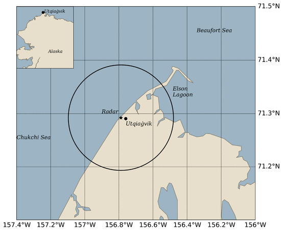
Figure 1.
Map of the study site and location of the CSIRS. The black circle marks the coastal radar range and the black start highlights the location of the coastal radar.
2.4. Floe Edge Detection Algorithms
We take advantage of the radar sensitivity to floe edges to identify ice floes and open water using the Canny edge detection operator [47] and the contour detection algorithm [48] from the open-source computer vision library OpenCV, which offers different tools to solve image-processing as well as face detection, feature tracking, and matching [49].
The Canny edge and Suzuki (finding contour) algorithms extract floe edges from the masked gray-scale images in six separate steps [47,48] (Figure 2). First, the land, Elson lagoon, and the digital boundary at the edge of the field of view are masked from all frames to limit the analysis to the ocean field of view that is resolved by the radar (Figure 3a,b). The landmask was produced using the NOAA’s National shoreline production available at https://www.fisheries.noaa.gov/inport/item/60548 (last accessed 21 August 2023). The NOAA’s National Shoreline Production land mask product has a spatial resolution of 5 m resolution for the dataset of the coastline near Utqiaġvik. The land mask product is then interpolated on the CSIRS grid at 24.7 m resolution. Finally, the coarser mask is used conjointly with the CSIRS images to blank the land and the Elson Lagoon. Second, a 5 × 5 Gaussian filter is applied to remove noise, followed by a convolution with the two-dimensional 3 × 3 Sobel kernel operator to compute edge gradients and directions. The Sobel operator, in the x-direction, is given by:
and is the transpose of . The edge gradient G in the direction can then be written as:
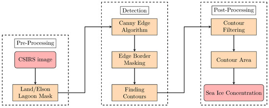
Figure 2.
Flow chart of the floe edge detection algorithm.
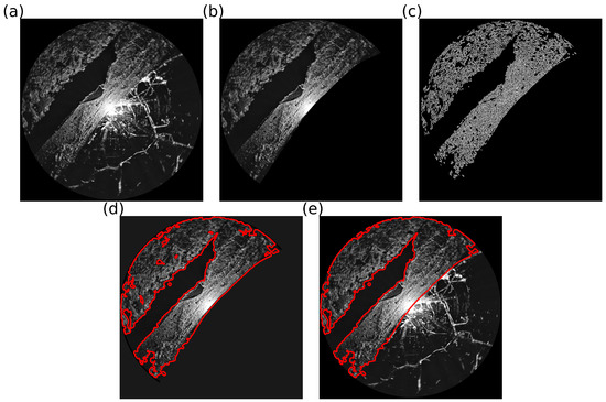
Figure 3.
Images from 11 March 2022, taken after each algorithm step: (a) initial image, (b) image with land removed, (c) the output of the Canny edge algorithm, (d) the contours, in red, found from the detected edges, and (e) the final sea ice contour.
Third, the edge gradients are refined using a non-maximum suppression step keeping only the local maximum in gradients. Pixels with a gradient magnitude larger than their two neighbors in the gradient direction are considered as possible edge pixels. Fourth, the floe edges are formed by applying a two-threshold hysteresis procedure (see Section 2.6 for optimization procedure), where pixels with a gradient larger than an upper threshold () are considered as an edge, and pixels with a gradient in between the lower and upper thresholds ( G ) are considered as an edge only if they are connected to another edge pixel [47,50]. A threshold below the lower threshold is always rejected. One pixel width edges result from the combination of the previous steps. Fifth, a binary mask is used to remove the radar image boundary where large gradients are present. The binary mask is created by first applying a threshold; the darker pixels with an intensity less than 5 are set to 0, and the others are assigned a maximum value of 1. An erosion is then performed to sharply identify the boundary of the darker region around the field of view of the radar and the interior of the radar image. The edges identified at the boundary or in the darker region are filtered out (Figure 3c). Sixth, the Suzuki algorithm is used to link the points identified as edges by the Canny edge algorithm [48]. Specifically, the edges are dilated by convoluting the image with a square kernel and with the pixel below the anchor point equal to the maximum value within the kernel square, resulting in well-defined (sharp gradient) edge segments that are all connected together [50] (Figure 3d).
2.5. Post-Processing
We first filter out (rare events of) closed contours within larger contours, assuming that they are primarily shadows behind ridges rather than open water. This is confirmed visually from inspection of the animated radar images for 10 scenes also analyzed by human analysts (see Section 2.6 for details), where detection of ice and open water is easier. In turn, the areas of low-radar return—in the shadow of ridges or covered by smooth ice inside edges—are marked as sea ice despite having a similar signature as open water [39] (Figure 3e). Finally, we calculate the (sea ice) area within each closed contour. The sea ice concentration is the ratio of the sea ice area to the total radar ocean field of view.
2.6. Parameters Optimization
Following [51], we use the sea ice edge analysis of fourteen radar frames by 10 human analysts from our research group as truth to optimize the two Canny edge thresholds and contour kernel. The analysts were specifically asked to identify the sea ice edge in every frame by manually drawing closed contours. Most of the analysts were not familiar with marine radar images. The dates were removed from the images so as to not bias the analysts in their interpretation of features identified on the image (e.g., no sea ice can be present in summer; therefore, it must be fog, or vice versa). The fourteen frames, selected in the 2022–2023 time span, are representative of the full range of sea ice conditions seen by the radar, i.e., 100% sea ice, 100% open water, and a mixture of open-water, landfast, and drifting ice (Figure 4). No fog-only frames were included in the subset of images to eliminate biases in the radar-derived SIC when low SIC values are present and because we are mostly interested in winter conditions. For each of those frames, the sea ice concentration was computed by first isolating the colored contours from the rest of the image and then using the finding contour algorithm presented earlier. The standard deviation between the analysts’ sea ice concentration for each frame is the inter-analyst error.
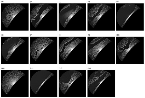
Figure 4.
Images analyzed by the analysts.
We iterated through the full parameter space for the lower () and upper () thresholds (0–255) and kernel dilation window size (3, 5, 7, 9, 11, 13), and ran the floe edge detection algorithm for every parameter combination to find the set that minimizes the root mean square error (RMSE) given by
where N is the total number of data points, A and are the radar and analyst’s SIC, and the slope of the best line fit between the analyst and algorithm is determined. We minimize the RMSE instead of the mean bias error (MBE),
because we emphasize precision over accuracy. The robustness of the optimized set of parameters was assessed using a leave-one-frame-out approach.
Finally, the CSIRS daily, weekly, and monthly mean SIC was calculated from each 4 min frame (a maximum of 360 when no missing values are present) in the 2022–2023 time period.
2.7. Comparison of SIC Products
We perform a point-by-point comparison of the 1 × 1 km sea ice edge from the NASA WorldView MODIS Terra (https://worldview.earthdata.nasa.gov) and a coarse-grained 1 km resolution CSIRS SIC for 15:09 local time (AKDT) 14 April 2022, a day when no clouds were present. To this end, areas of 50 cells (1 km/24.7 m) are combined to form the coarse-grain sea ice concentration estimate of ∼1 km resolution. The coarse-grain estimate is obtained by running the floe edge detection algorithm on the CSIRS frame closest to the MODIS Terra detection time (15:09 local AKDT time). Each pixel inside the radar edge contours is identified as sea ice or open water using a binary mask (0 or 1). The coarse-grain estimate is interpolated on the same grid as the merged MODIS-AMSR2 SIC dataset using regridded 1 km resolution central longitude and latitude. Finally, each point is compared by computing the Pearson correlation coefficient between the estimated 1 km CSIRS SIC and the merged MODIS-AMSR2.
For the CDR dataset, the error estimate for SIC near the coastline is calculated from only one grid cell in the field of view of the marine radar, and, therefore, no spread estimate is possible (Figure 5). We compute the Pearson correlation coefficient between the CDR, MODIS-AMSR2, and CSIRS datasets by first removing the 31-day running mean to filter the low-frequency signals.
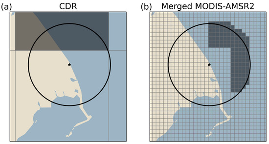
Figure 5.
CDR (a) and merged MODIS-AMSR2 (b) grid cells used for the comparison with the marine radar. Utqiaġvik and the radar range are marked with a black star and circle.
3. Results
3.1. Optimization/Validation
The minimum RMSE and departure from a perfect (1:1) fit for all thresholds and kernels tested in the parameter space range from 0.03 to 0.06 and from 0.060 to 0.12, respectively (Figure 6). The best line fit between the Canny edge algorithm and the analysis of 14 images from 10 analysts is obtained with the 11 × 11 kernel, and (Figure 6a). The resulting slope and intercept of the linear regression are 0.94 and 0.036, respectively. An optimization based on the RMSE instead results in a small reduction in error (RMSE = 0.035) but a large maximum bias (=0.1 for SIC = 1) and is, therefore, not the preferred option (Figure 6a). The inter-analyst error (=0.026)—a measure of the error on the “truth”—is small compared with the RMSE, indicating that most of the difference between the kernels can be attributed to the algorithm (Figure 6b,c). The inter-analyst differences, however, still introduce some variability in the floe edge algorithm optimized parameters. For instance, the low-return area offshore of the leads, a mixture of a large number of small floes surrounded by open water and fog, was identified as ice by some and open water by others (Figure 4 Frames 7–10–14, Figure 6c and see Supplementary Materials Figure S1). Finally, removing one frame at a time in the optimization of the algorithm leads to a distribution of best line fit slopes with a standard deviation of 0.005 (and a mean equal to the optimal slope reported above, Figure 6d). This provides an estimate of the robustness of the method short of increasing the number of analysts’ estimates (Figure 4).
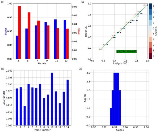
Figure 6.
(a) Minimum RMSE (red) and the corresponding best 1:1 line fit (blue) for each kernel, (b) scatter plot of SIC derived from the radar images with the optimal set of parameters and SIC from the 10 analysts (colorbar), including the best-line fit (green line), (c) the analyst standard deviation (STD) for each analyzed frame, and (d) histogram of the departure of the best 1:1 line fit when removing one-by-one the analyzed frame. Note that the blue axis in (a) does not start at 0. Each of the horizontal lines represent a different image in (b). The inter-analyst averaged error of 0.026 is represented by the dashed line in (c).
The detection algorithm with the optimal parameter successfully identifies most of the sea ice edge features observed by MODIS Terra on 14 April 2022, under cloud-free conditions, including the rugged features of the sea ice edge present in both images (Figure 7a,b). The open water and the narrow band of open water southwest and directly in front of the radar are well identified. The open water to the north and the water between the broken floes to the north of the radar image, however, are missed by the algorithm (Figure 7a,b). This limitation is caused by the fog-like features present at the center of the image, which prevents the detection of all floe edges. We note that the analysts also interpreted, at times, a mixture of floe and open water as full sea ice cover. Finally, the coarse-grain CSIRS SIC estimate correlates well with the daily merged MODIS-AMSR2 SIC, with the correlation coefficient exceeding 0.6 for most of the day. At the time of maximum correlation (r∼), the point-by-point comparison of the coarse-grained and the merged MODIS-AMSR2 gives a best line fit with slope of 0.43 and RMSE of 0.12, with open water and fully ice-covered grid cells over- and under-estimated by the MODIS-AMSR2 product, respectively (Figure 7d). The drop in correlation during the middle of the day is presumably due to the swaths composing the merged MODIS-AMSR2 SIC not being taken at this time. Overall, the detection algorithm can identify most sea ice edges present in the MODIS image, considering that the exact acquisition time of the merged MODIS-AMSR2 SIC passing over the marine radar field of view is unknown.
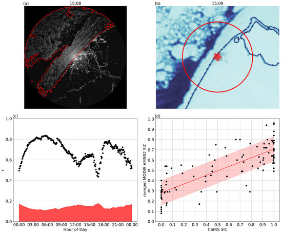
Figure 7.
(a) Nearly synchronous marine radar image, including sea ice edge (red) from the detection algorithm and at 15:09 local time (AKDT). (b) MODIS Terra image at 15:09 AKDT. (c) Time series of Pearson correlation coefficient (r) between all coarse-grained (1 km) 4 min images (360 in total) CSIRS SIC and the merged MODIS-AMSR2 SIC for 14 April 2022. The red shading corresponds to the 95% confidence interval. (d) Scatter plot of the CSIRS SIC with the merged MODIS-AMSR2 for the time of maximum correlation at 6:00 AKDT. The best line fit is given by and the red shading corresponds to the RMSE of 0.12.
3.2. CSIRS Reconstructed Sea Ice Concentration
The CDR data and the merged MODIS-AMSR2 overestimate SIC with respect to the CSIRS with an MBE equal to −0.10 and , respectively (Table 1 and Figure 8a). The correlation coefficients between the daily CDR, MODIS-AMSR2, and the reconstructed SIC from CSIRS are low (r = 0.18) and moderate (r = 0.54), both significant at the 95% level, and the RMSE errors are 0.34 and 0.29, respectively (Figure 1). In winter, the CDR generally underestimates short-lived low SIC (breakout) events, most notably in early winter 2023 (January–February 2023), while MODIS-AMSR2 SICs are in general agreement with the observed values (Figure 8a). In the break-up period (June–July 2022), CDR is in general agreement with observations, while during the freeze-up (December 2022–January 2023), both satellites lead the observed ice onset by approximately 10 days, perhaps due to land contamination with an earlier onset of snow presence on land [52]. In the summer, the algorithm incorrectly identifies clouds as sea ice with reconstructed SICs ranging between 20–25%. The CDR SIC, on the other hand, correctly identified open water during this period (Figure 8). Finally, the weekly and monthly running averages show an increase in correlation to 0.68 and 0.59, and 0.26 and 0.71, for MODIS-AMSR2 and CDR, respectively (Figure 1).

Table 1.
Pearson correlation coefficient (r), root mean square error (RMSE), and mean bias error (MBE) for the daily, 7-day and 31-day running mean CSIRS SIC, CDR, and merged MODIS-AMSR2 SIC for 2022 and 2023.
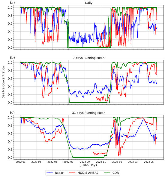
Figure 8.
Daily (a), 7-day running mean (b), and 31-day running mean (c) time series of the SIC derived from the radar (blue), the CDR (green), and the merged MODIS-AMSR2 (red) for 2022 to 2023 as a function of the Julian days starting 1 January 2022. The holes in the time series represent the non-availability of the data.
4. Discussion
To a first order, both the CDR and the merged MODIS-AMSR2 datasets capture the same seasonality of SIC at Utqiaġvik as the CSIRS. In mid- to late-winter, spring, and early summer, the CDR SIC is in good agreement with the CSIRS SIC, while the merged MODIS-AMSR2 is in better agreement in the fall freeze-up and early winter. In the early winter of 2023, the CDR underestimates break-up events, while the MODIS-AMSR2 under-estimates the CSIRS SIC in mid- to late-winter, presumably due to the AMSR2 mask not capturing the landfast ice area near the coast (see Figure 5). In the summer, the Canny edge algorithm interprets the presence of fog and clouds as sea ice near the coast, leading to a positive bias in the reconstruction.
The floe edge detection algorithm’s performance depends on the images’ gradient in color, and hence performs better when no fog and clear open water areas between the larger unbroken plates of sea ice are present in the images. Consequently, during the summer and fall when fog is mostly present due to large air–sea temperature differences, larger errors are present in the detection algorithm. Fog can also blur the contrast between different ice floes, or even be interpreted as sea ice in the summer; in both cases, it leads to errors in the reconstructed open water/ice areas. These are periods, however, when there are no uncertainties as to the surface conditions derived from satellite remote sensing or from direct observations, and the radar is not used by the community or ship navigators. The misinterpretation of shadows behind ridges or open water areas populated by a number of small floes (e.g., Figure 7a,b) is another significant source of error in the winter when the analysts and the algorithm disagreed the most (Figure 6c). In such situations, the open water area is smaller and the gradient less well defined, and the algorithm considers the area populated by a large number of small floes as open water. Adding a fog-type frame to the optimization resulted in stronger disagreements between the optimized parameters and the analysts, particularly in the winter when the marine radar is mostly used.
5. Conclusions
We present a six-step floe edge detection algorithm based on the Canny edge and the Suzuki finding contour algorithms. The model was optimized by reconstructing the ice edge to that made by ten analysts for 14 different images, which included a wide range of sea ice conditions and features. The detection algorithm was applied to 4-minute snapshots between 2022 and mid-2023 to obtain a daily CSIRS SIC estimate and 7-day and 31-day running averages. To the best of the authors’ knowledge, this is the first time that open water and sea ice are estimated directly from marine radar images.
The error (or standard deviation) on the sea ice concentration from the analysts is , with the largest error () in images where the contrasts were reduced by the presence of fog and/or a mixture of small floes and open water. The optimal set of parameters ( and kernel rank of 11 × 11) for the algorithm were chosen such that the slope of the best line fit between the analysts to the detection algorithm was closest to one (slope = and RMSE = ∼). The optimal slope from the optimization procedure is robust to the exact choice of images, with an estimated error of 0.0052 estimated from a leave-one-out approach. The difficulty in identifying sea ice when fog is present or when a large number of small floes are surrounded by open water was confirmed from a comparison with a high-resolution (250 m) image from MODIS Terra.
The floe edge detection algorithm successfully identifies sea ice and open water, including break-up events under all conditions, when compared to the merged MODIS-AMSR2 and CDR SIC datasets. The daily, 7-day, and 31-day average reconstructed SICs correlate with the MODIS-AMSR2 and CDR SICs with correlation coefficients of 0.54, 0.68, 0.59 and 0.18, 0.26, 0.72, respectively. CDR and merged MODIS-AMSR2 overestimate the daily SIC with a mean bias error (MBE) of −0.10 and −7.0 × . The MODIS-AMSR2 SICs mostly agree with that of the marine radar during the winter and spring, including break-up events resulting in excursions of lower SIC when break-up events are present. The CDR SICs, on the other hand, are in good agreement with the marine radar during the melt season but underestimate the low SIC excursions during winter. In summer, the algorithm produces SICs with a positive bias of 20–25% when fog is present, and the contrast in the images is reduced, while the CDR SICs correctly interpret the presence of open water [26,38].
In summary, marine radar images and a floe detection algorithm can be used jointly to derive SIC at a spatial and temporal time scale meaningful to community users and assess uncertainties associated with land contamination in low- and high-resolution satellite products. Raising the coastal radar height above ground (if at all possible) and, therefore, radar range would provide a valuable dataset for the evaluation of land contamination in low-resolution satellite-derived SIC and would reduce the shadow effect from nearby ridges. Two new marine radars were installed recently in Nome and Gambell (AK). Future work includes testing the proposed algorithm on the new radar images from two locations with very different sea ice regimes and implementing an edge-tracking feature in time to better estimate the sea ice concentration. Future work also includes considering the texture of the images to reduce the false detection rates [21,53] when fog or haze is present. Given that the MODIS mission is nearing its end, the proposed CSIRS SIC could be used to evaluate other high-resolution satellite products, such as the Visible Infrared Imaging Radiometer (VIIRS) SIC datasets [54,55].
Supplementary Materials
The following supporting information can be downloaded at: https://www.mdpi.com/article/10.3390/rs16183357/s1, Figure S1: Analysis of snapshot 14 by the 10 analysts.
Author Contributions
Conceptualization, L.B.T., F.S.-D. and K.P.L.M.T.-G.; methodology, L.B.T. and F.S.-D.; software, F.S.-D.; validation, L.B.T. and F.S.-D.; formal analysis, F.S.-D., L.B.T. and A.R.M.; investigation, L.B.T. and F.S.-D.; resources, F.S.-D. and L.B.T.; data curation, F.S.-D. and A.R.M.; writing—original draft preparation, F.S.-D.; writing—review and editing, L.B.T., A.R.M. and K.P.L.M.T.-G.; visualization, F.S.-D.; supervision, L.B.T.; project administration, L.B.T.; funding acquisition, L.B.T. and A.R.M. All authors have read and agreed to the published version of the manuscript.
Funding
This project is a contribution to the Navigating the New Arctic project entitled ARC-NAV: Arctic Robust Communities-Navigating Adaptation to Variability, funded by the National Science Foundation–Office of Polar Program (project #1928126, 1928259) awarded to Tremblay and Mahoney, and a Discovery grant from the Natural Sciences and Engineering Research Council, awarded to Tremblay. This work also benefited from the academic and financial support of McGill University and Québec–Océan.
Data Availability Statement
The original contributions presented in the study are included in the article/Supplementary Materials; further enquiries can be directed to the corresponding author/s. The CSIRS images, the (Near-Real-Time)-CDR, and the CDR Sea Ice Concentration dataset are publicly available at https://seaice.alaska.edu/gi/observatories/barrow_radar/ (last accessed 21 August 2023), https://nsidc.org/data/g10016/versions/2#anchor-data-access-tools (last accessed 21 August 2023), https://nsidc.org/data/g02202/versions/4#anchor-documentation (last accessed 21 August 2023), respectively. The code produced for this study can be made publicly available if asked.
Acknowledgments
Felix St-Denis is thankful to the Institute of Environmental Physics, University of Bremen, for the provision of the merged MODIS-AMSR2 sea ice concentration data at https://data.seaice.uni-bremen.de/modis_amsr2 (last accessed 20 June 2024). Felix St-Denis is grateful to the Fond de Recherche du Québec Nature et Technologie (FRQNT), the Natural Sciences and Engineering Research Council of Canada (NSERC), and the North Slope Borough of Alaska (Eben Hopson Fellowship) for scholarships received during the course of this work. Felix St-Denis is grateful for the sea ice group to have willingly taken part in this study. Félix St-Denis and Bruno Tremblay thank Joshua Jones for the insightful comments about the work presented in this paper and Samuel George for the frontline work with the CSIRS.
Conflicts of Interest
The authors declare no conflicts of interest.
References
- Ford, J.D.; Willox, A.C.; Chatwood, S.; Furgal, C.; Harper, S.; Mauro, I.; Pearce, T. Adapting to the Effects of Climate Change on Inuit Health. Am. J. Public Health 2014, 104, e9–e17. [Google Scholar] [CrossRef] [PubMed]
- Box, J.E.; Colgan, W.T.; Christensen, T.R.; Schmidt, N.M.; Lund, M.; Parmentier, F.J.W.; Brown, R.; Bhatt, U.S.; Euskirchen, E.S.; Romanovsky, V.E.; et al. Key indicators of Arctic climate change: 1971–2017. Environ. Res. Lett. 2019, 14, 045010. [Google Scholar] [CrossRef]
- Middleton, J.; Cunsolo, A.; Jones-Bitton, A.; Wright, C.J.; Harper, S.L. Indigenous mental health in a changing climate: A systematic scoping review of the global literature. Environ. Res. Lett. 2020, 15, 053001. [Google Scholar] [CrossRef]
- Middleton, J.; Cunsolo, A.; Jones-Bitton, A.; Shiwak, I.; Wood, M.; Pollock, N.; Flowers, C.; Harper, S.L. “We’re people of the snow:” Weather, climate change, and Inuit mental wellness. Soc. Sci. Med. 2020, 262, 113137. [Google Scholar] [CrossRef] [PubMed]
- Meier, W.; Stroeve, J. An Updated Assessment of the Changing Arctic Sea Ice Cover. Oceanography 2022, 35, 10–19. [Google Scholar] [CrossRef]
- Comiso, J.C. Large Decadal Decline of the Arctic Multiyear Ice Cover. J. Clim. 2012, 25, 1176–1193. [Google Scholar] [CrossRef]
- Ford, J.D.; Pearce, T.; Canosa, I.V.; Harper, S. The rapidly changing Arctic and its societal implications. WIREs Clim. Chang. 2021, 12, e735. [Google Scholar] [CrossRef]
- Hauser, D.D.W.; Whiting, A.V.; Mahoney, A.R.; Goodwin, J.; Harris, C.; Schaeffer, R.J.; Schaeffer, R.; Laxague, N.J.M.; Subramaniam, A.; Witte, C.R.; et al. Co-production of knowledge reveals loss of Indigenous hunting opportunities in the face of accelerating Arctic climate change. Environ. Res. Lett. 2021, 16, 095003. [Google Scholar] [CrossRef]
- Ford, J.D. Dangerous climate change and the importance of adaptation for the Arctic’s Inuit population. Environ. Res. Lett. 2009, 4, 024006. [Google Scholar] [CrossRef]
- Ford, J.D.; Clark, D.; Pearce, T.; Berrang-Ford, L.; Copland, L.; Dawson, J.; New, M.; Harper, S.L. Changing access to ice, land and water in Arctic communities. Nat. Clim. Chang. 2019, 9, 335–339. [Google Scholar] [CrossRef]
- Laidler, G.J.; Ford, J.D.; Gough, W.A.; Ikummaq, T.; Gagnon, A.S.; Kowal, S.; Qrunnut, K.; Irngaut, C. Travelling and hunting in a changing Arctic: Assessing Inuit vulnerability to sea ice change in Igloolik, Nunavut. Clim. Chang. 2009, 94, 363–397. [Google Scholar] [CrossRef]
- Gearheard, S.F. The Meaning of Ice: People and Sea Ice in Three Arctic Communities; International Polar Institute Press: Hanover, NH, USA, 2013. [Google Scholar]
- Druckenmiller, M.L.; Eicken, H.; George, J.C.; Brower, L. Trails to the whale: Reflections of change and choice on an Iñupiat icescape at Barrow, Alaska. Polar Geogr. 2013, 36, 5–29. [Google Scholar] [CrossRef]
- Ludwig, V.; Spreen, G.; Haas, C.; Istomina, L.; Kauker, F.; Murashkin, D. The 2018 North Greenland polynya observed by a newly introduced merged optical and passive microwave sea-ice concentration dataset. Cryosphere 2019, 13, 2051–2073. [Google Scholar] [CrossRef]
- Parkinson, C.L.; Cavalieri, D.J. Arctic sea ice 1973–1987: Seasonal, regional, and interannual variability. J. Geophys. Res. Ocean. 1989, 94, 14499–14523. [Google Scholar] [CrossRef]
- Canadian Ice Service. Canadian Ice Service Arctic Regional Sea Ice Charts in SIGRID-3 Format; Version 1; NSIDC: Boulder, CO, USA, 2009. [Google Scholar] [CrossRef]
- Zakhvatkina, N.; Smirnov, V.; Bychkova, I. Satellite SAR Data-based Sea Ice Classification: An Overview. Geosciences 2019, 9, 152. [Google Scholar] [CrossRef]
- Komarov, A.S.; Barber, D.G. Sea Ice Motion Tracking from Sequential Dual-Polarization RADARSAT-2 Images. IEEE Trans. Geosci. Remote Sens. 2014, 52, 121–136. [Google Scholar] [CrossRef]
- Korosov, A.A.; Rampal, P. A Combination of Feature Tracking and Pattern Matching with Optimal Parametrization for Sea Ice Drift Retrieval from SAR Data. Remote Sens. 2017, 9, 258. [Google Scholar] [CrossRef]
- Dierking, W. Sea Ice Monitoring by Synthetic Aperture Radar. Oceanography 2013, 26, 100–111. [Google Scholar] [CrossRef]
- Soh, L.K.; Tsatsoulis, C. Texture analysis of SAR sea ice imagery using gray level co-occurrence matrices. IEEE Trans. Geosci. Remote Sens. 1999, 37, 780–795. [Google Scholar] [CrossRef]
- Ochilov, S.; Clausi, D.A. Operational SAR Sea-Ice Image Classification. IEEE Trans. Geosci. Remote Sens. 2012, 50, 4397–4408. [Google Scholar] [CrossRef]
- Ludwig, V.; Spreen, G.; Pedersen, L.T. Evaluation of a New Merged Sea-Ice Concentration Dataset at 1 km Resolution from Thermal Infrared and Passive Microwave Satellite Data in the Arctic. Remote Sens. 2020, 12, 3183. [Google Scholar] [CrossRef]
- Nicolaus, M.; Perovich, D.K.; Spreen, G.; Granskog, M.A.; von Albedyll, L.; Angelopoulos, M.; Anhaus, P.; Arndt, S.; Belter, H.J.; Bessonov, V.; et al. Overview of the MOSAiC expedition: Snow and sea ice. Elem. Sci. Anthr. 2022, 10, 000046. [Google Scholar] [CrossRef]
- Lund, B.; Graber, H.C.; Persson, P.O.G.; Smith, M.; Doble, M.; Thomson, J.; Wadhams, P. Arctic Sea Ice Drift Measured by Shipboard Marine Radar. J. Geophys. Res. Ocean. 2018, 123, 4298–4321. [Google Scholar] [CrossRef]
- Jones, J.; Eicken, H.; Mahoney, A.; Mv, R.; Kambhamettu, C.; Fukamachi, Y.; Ohshima, K.I.; George, J.C. Landfast sea ice breakouts: Stabilizing ice features, oceanic and atmospheric forcing at Barrow, Alaska. Cont. Shelf Res. 2016, 126, 50–63. [Google Scholar] [CrossRef]
- Karvonen, J. Tracking the motion of recognizable sea-ice objects from coastal radar image sequences. Ann. Glaciol. 2013, 54, 41–49. [Google Scholar] [CrossRef]
- Karvonen, J. Virtual radar ice buoys—A method for measuring fine-scale sea ice drift. Cryosphere 2016, 10, 29–42. [Google Scholar] [CrossRef]
- Oikkonen, A.; Haapala, J.; Lensu, M.; Karvonen, J. Sea ice drift and deformation in the coastal boundary zone. Geophys. Res. Lett. 2016, 43, 10303–10310. [Google Scholar] [CrossRef]
- Shirasawa, K.; Ebuchi, N.; Leppäranta, M.; Takatsuka, T. Ice-edge detection from Japanese C-band radar and high-frequency radar coastal stations. Ann. Glaciol. 2013, 54, 59–64. [Google Scholar] [CrossRef]
- Mv, R.; Jones, J.; Eicken, H.; Kambhamettu, C. Extracting Quantitative Information on Coastal Ice Dynamics and Ice Hazard Events from Marine Radar Digital Imagery. IEEE Trans. Geosci. Remote Sens. 2013, 51, 2556–2570. [Google Scholar] [CrossRef]
- O’Connell, B.J. Marine Radar for Improved Ice Detection. In Proceedings of the SNAME 8th International Conference and Exhibition on Performance of Ships and Structures in Ice, Banff, AB, Canada, 22–28 July 2008; p. D031S011R002. [Google Scholar] [CrossRef]
- Lu, P.; Li, Z.; Shi, L.; Huang, W. Marine radar observations of iceberg distribution in the summer Southern Ocean. Ann. Glaciol. 2013, 54, 35–40. [Google Scholar] [CrossRef]
- Tabata, T. Sea-ice Reconnaissance by Radar. J. Glaciol. 1975, 15, 215–224. [Google Scholar] [CrossRef][Green Version]
- Flock, W.L. Monitoring Open Water and Sea Ice in the Bering Strait by Radar. IEEE Trans. Geosci. Electron. 1977, 15, 196–202. [Google Scholar] [CrossRef]
- Haykin, S.; Currie, B.; Lewis, E.; Nickerson, K. Surface-based radar imaging of sea ice. Proc. IEEE 1985, 73, 233–251. [Google Scholar] [CrossRef]
- Shapiro, L.H.; Metzner, R.C. Nearshore Iceconditions from Radar Data, Point Barrow, Alaska; University of Alaska Fairbanks: Fairbanks, AK, USA, 1989. [Google Scholar]
- Mahoney, A.; Eicken, H.; Shapiro, L. How fast is landfast sea ice? A study of the attachment and detachment of nearshore ice at Barrow, Alaska. Cold Reg. Sci. Technol. 2007, 47, 233–255. [Google Scholar] [CrossRef]
- Mahoney, A.R.; Eicken, H.; Fukamachi, Y.; Ohshima, K.I.; Simizu, D.; Kambhamettu, C.; Rohith, M.; Hendricks, S.; Jones, J. Taking a look at both sides of the ice: Comparison of ice thickness and drift speed as observed from moored, airborne and shore-based instruments near Barrow, Alaska. Ann. Glaciol. 2015, 56, 363–372. [Google Scholar] [CrossRef]
- Kettle, N.P.; Abdel-Fattah, D.; Mahoney, A.R.; Eicken, H.; Brigham, L.W.; Jones, J. Linking Arctic system science research to decision maker needs: Co-producing sea ice decision support tools in Utqiaġvik, Alaska. Polar Geogr. 2020, 43, 206–222. [Google Scholar] [CrossRef]
- Meier, W.; Fetterer, F.; Windnagel, A.; Stewart, S. NOAA/NSIDC Climate Data Record of Passive Microwave Sea Ice Concentration; Version 4; NSIDC: Boulder, CO, USA, 2021. [Google Scholar] [CrossRef]
- Meier, W.; Fetterer, F.; Windnagel, A.; Stewart, S. Near-Real-Time NOAA/NSIDC Climate Data Record of Passive Microwave Sea Ice Concentration; Version 2; NSIDC: Boulder, CO, USA, 2021. [Google Scholar] [CrossRef]
- Cavalieri, D.J.; Gloersen, P.; Campbell, W.J. Determination of sea ice parameters with the NIMBUS 7 SMMR. J. Geophys. Res. Atmos. 1984, 89, 5355–5369. [Google Scholar] [CrossRef]
- Comiso, J.C. Characteristics of Arctic winter sea ice from satellite multispectral microwave observations. J. Geophys. Res. 1986, 91, 975. [Google Scholar] [CrossRef]
- Kern, S.; Lavergne, T.; Notz, D.; Pedersen, L.T.; Tonboe, R. Satellite passive microwave sea-ice concentration data set inter-comparison for Arctic summer conditions. Cryosphere 2020, 14, 2469–2493. [Google Scholar] [CrossRef]
- Druckenmiller, M.L.; Eicken, H.; Johnson, M.A.; Pringle, D.J.; Williams, C.C. Toward an integrated coastal sea-ice observatory: System components and a case study at Barrow, Alaska. Cold Reg. Sci. Technol. 2009, 56, 61–72. [Google Scholar] [CrossRef]
- Canny, J. A Computational Approach to Edge Detection. IEEE Trans. Pattern Anal. Mach. Intell. 1986, PAMI-8, 679–698. [Google Scholar] [CrossRef]
- Suzuki, S.; be, K. Topological structural analysis of digitized binary images by border following. Comput. Vision Graph. Image Process. 1985, 30, 32–46. [Google Scholar] [CrossRef]
- Bradski, G. The opencv library. Dr. Dobb’s J. Softw. Tools Prof. Program. 2000, 25, 120–123. [Google Scholar]
- Bradski, G.R.; Kaehler, A. Learning OpenCV: Computer Vision with the OpenCV Library, 1st ed.; Software That Sees; O’Reilly: Beijing, China, 2011. [Google Scholar]
- Cheng, A.; Casati, B.; Tivy, A.; Zagon, T.; Lemieux, J.F.; Tremblay, L.B. Accuracy and inter-analyst agreement of visually estimated sea ice concentrations in Canadian Ice Service ice charts using single-polarization RADARSAT-2. Cryosphere 2020, 14, 1289–1310. [Google Scholar] [CrossRef]
- Parkinson, C.L. Spatial patterns of increases and decreases in the length of the sea ice season in the north polar region, 1979–1986. J. Geophys. Res. Ocean. 1992, 97, 14377–14388. [Google Scholar] [CrossRef]
- Clausi, D.A. Comparison and fusion of co-occurrence, Gabor and MRF texture features for classification of SAR sea-ice imagery. Atmos.-Ocean 2001, 39, 183–194. [Google Scholar] [CrossRef]
- Hoffman, J.P.; Ackerman, S.A.; Liu, Y.; Key, J.R. A 20-Year Climatology of Sea Ice Leads Detected in Infrared Satellite Imagery Using a Convolutional Neural Network. Remote Sens. 2022, 14, 5763. [Google Scholar] [CrossRef]
- Dworak, R.; Liu, Y.; Key, J.; Meier, W.N. A Blended Sea Ice Concentration Product from AMSR2 and VIIRS. Remote Sens. 2021, 13, 2982. [Google Scholar] [CrossRef]


Disclaimer/Publisher’s Note: The statements, opinions and data contained in all publications are solely those of the individual author(s) and contributor(s) and not of MDPI and/or the editor(s). MDPI and/or the editor(s) disclaim responsibility for any injury to people or property resulting from any ideas, methods, instructions or products referred to in the content. |
© 2024 by the authors. Licensee MDPI, Basel, Switzerland. This article is an open access article distributed under the terms and conditions of the Creative Commons Attribution (CC BY) license (https://creativecommons.org/licenses/by/4.0/).