Relationship between Vegetation and Soil Moisture Anomalies Based on Remote Sensing Data: A Semiarid Rangeland Case

Abstract

The dynamic of rangelands results from complex interactions between vegetation, soil, climate, and human activity. This scenario makes rangeland’s condition challenging to monitor, and degradation assessment should be carefully considered when studying grazing pressures. In the present work, we study the interaction of vegetation and soil moisture in semiarid rangelands using vegetation and soil moisture indices. We aim to study the feasibility of using soil moisture negative anomalies as a warning index for vegetation or agricultural drought. Two semiarid agricultural regions were selected in Spain for this study: Los Vélez (Almería) and Bajo Aragón (Teruel). MODIS images, with 250 m and 500 m spatial resolution, from 2002 to 2019, were acquired to calculate the Vegetation Condition Index (VCI) and the Water Condition Index (WCI) based on the Normalised Difference Vegetation Index (NDVI) and soil moisture component (W), respectively. The Optical Trapezoid Model (OPTRAM) estimated this latter W index. From them, the anomaly (Z-score) for each index was calculated, being $Z_{VCI}$ and $Z_{WCI}$, respectively. The probability of coincidence of their negative anomalies was calculated every 10 days (10-day periods). The results show that for specific months, the $Z_{WCI}$ had a strong probability of informing in advance, where the negative $Z_{VCI}$ will decrease. Soil moisture content and vegetation indices show more similar dynamics in the months with lower temperatures (from autumn to spring). In these months, given the low temperatures, precipitation leads to vegetation growth. In the following months, water availability depends on evapotranspiration and vegetation type as the temperature rises and the precipitation falls. The stronger relationship between vegetation and precipitation from autumn to the beginning of spring is reflected in the feasibility of $Z_{WCI}$ to aid the prediction of $Z_{VCI}$. During these months, using $Z_{WCI}$ as a warning index is possible for both areas studied. Notably, November to the beginning of February showed an average increase of 20–30% in the predictability of vegetation anomalies, knowing moisture soil anomalies four lags in advance. We found other periods of relevant increment in the predictability, such as March and April for Los Vélez, and from July to September for Bajo Aragón.

1. Introduction

Precipitation and temperature directly influence water balance, causing changes in soil moisture (SM) regime, which, in turn, influences plant growth. Temperature also directly affects plant phenology and growth. Thus, SM is widely recognised as a critical parameter that links precipitation, temperature, evapotranspiration, and vegetation status. The most common vegetation index to assess vegetation status is the Normalised Difference Vegetation Index (NDVI). Adegoke and Carleton [1] aimed to show the link between NDVI and water soil content with different lags. In this study, stronger relations were obtained with SM data that lagged by up to 8 weeks with respect to the vegetation index, implying that SM may be a valuable predictor of warm season satellite-derived vegetation conditions. Recently, Felegari et al. [2] showed that plant indices such as NDVI have a delayed response to SM. In most cases, SM data and other meteorological characteristics strongly correlate with these indices in a short period. In a related study, Sharma et al. [3] examined the trends in MODIS/TERRA derived NDVI and its correlation with Land Surface Temperature (LST), SM, and precipitation over Gautam Buddh Nagar (India), during the period 2005–2018. The correlation between NDVI and LST was observed to be higher than the correlation of NDVI with SM and precipitation.

The difference between surface soil layers and root-zone soil must be noted when studying SM content [4], even though a strong correlation has been shown between these layers [5,6]. Different responses of NDVI to SM content are found among distinct vegetation types, especially between humid and arid or semiarid areas. These differences are due to the disparities among these areas at root-zone soils and surface soil layers [1,7,8]. NDVI has been shown to have strong links with root-zone SM and surface SM in grassland and shrubland in semiarid regions [8,9,10].

Droughts are often divided into four major types: meteorological, agricultural, hydrological, and socioeconomic. Meteorological drought is defined as a reduction of precipitation. Agricultural drought occurs when plants do not have enough available water to meet their requirements; therefore, this drought varies based on the vegetation type. Since this is vegetation specific, some soil water deficits may affect vegetation differently. Typically, there is a lag between soil water deficit and how this is reflected in the vegetation with shorter or wider periods. Hydrological droughts occur when the water moving through the ground is significantly reduced. Finally, socioeconomic droughts occur when a drought affects a community’s supply of goods and services. These droughts are sequential in time, increasing the complexity of their impacts and conflicts [11,12,13,14].

Remote sensing observation can monitor drought-related variables and assess their effects and impacts from an ecosystem perspective [7]. Precipitation has been studied with several indices [15,16], such as the Standardised Precipitation Index (SPI) [17], Effective Drought Index (EDI) [18], and Percent Normal Precipitation Index (PNPI) [19]. Several indices have been developed to estimate SM [20,21], such as the Standardised Soil Moisture Index (SSI) [22], Soil Moisture Percentile (SMP) [21,23], and OPTRAM (OPtical TRapezoid Model) [24,25]. Several works have shown that OPTRAM could be used to estimate SM with reasonable accuracy at large scales [24,25,26] and at field scales with ground references measurements [6,27,28].

As the drought types are sequential, an alarm index can be developed before more damage is caused. Drought indicators represent different stages of the hydrological cycle, such as precipitation or SM, and later impacts can be perceived in vegetation and water stress. How each stage behaves depends on the particular vegetation or ecosystem. Droughts cannot be avoided, but their impacts can be reduced by preparing for them. In this respect, different combined indicators that present indices with warning thresholds have been defined [22,29,30,31,32,33]. Early warning indices can provide a drought probability that can be used as a management tool. A proactive approach can be taken in drought risk management using different risk reduction instruments at different farm or government levels. These instruments include insurance, irrigation schemes, and budget releases. Despite presenting different challenges, early warning systems have already been used in the past [34,35]. Azhdari et al. [36] recently worked on a combined multivariate index named the Joint Deficit Hydro-meteorological Index (JDHMI) to monitor hydro-meteorological drought at a watershed scale. They estimated conditional probabilities to provide practical information for forecasting drought conditions. Hao et al. [37] investigated the conditional probability of vegetation decline under different climate conditions in a similar line of work. Another related study was carried out by Ribeiro et al. [38]. They used a bivariate copula approach to model joint probability distributions describing the amount of dependence between drought conditions and crop yield anomalies. Recently, Sanz et al. [39] pointed out that conditional probability could be applied to capture the causality between water availability and vegetation anomalies.

The first goal of this research is to better understand the relationships between vegetation and SM content indices in semiarid rangelands as a complex agricultural dynamic system. The second goal is to study the feasibility of using anomalies in SM (measured by the $Z_{WCI}$) as an advanced warning index to predict anomalies in the vegetation activity, measured by the $Z_{VCI}$. To accomplish these two goals, two semiarid rangelands were selected in Spain, Los Vélez in Almería province and Bajo Aragón in Teruel province.

2. Material and Methods

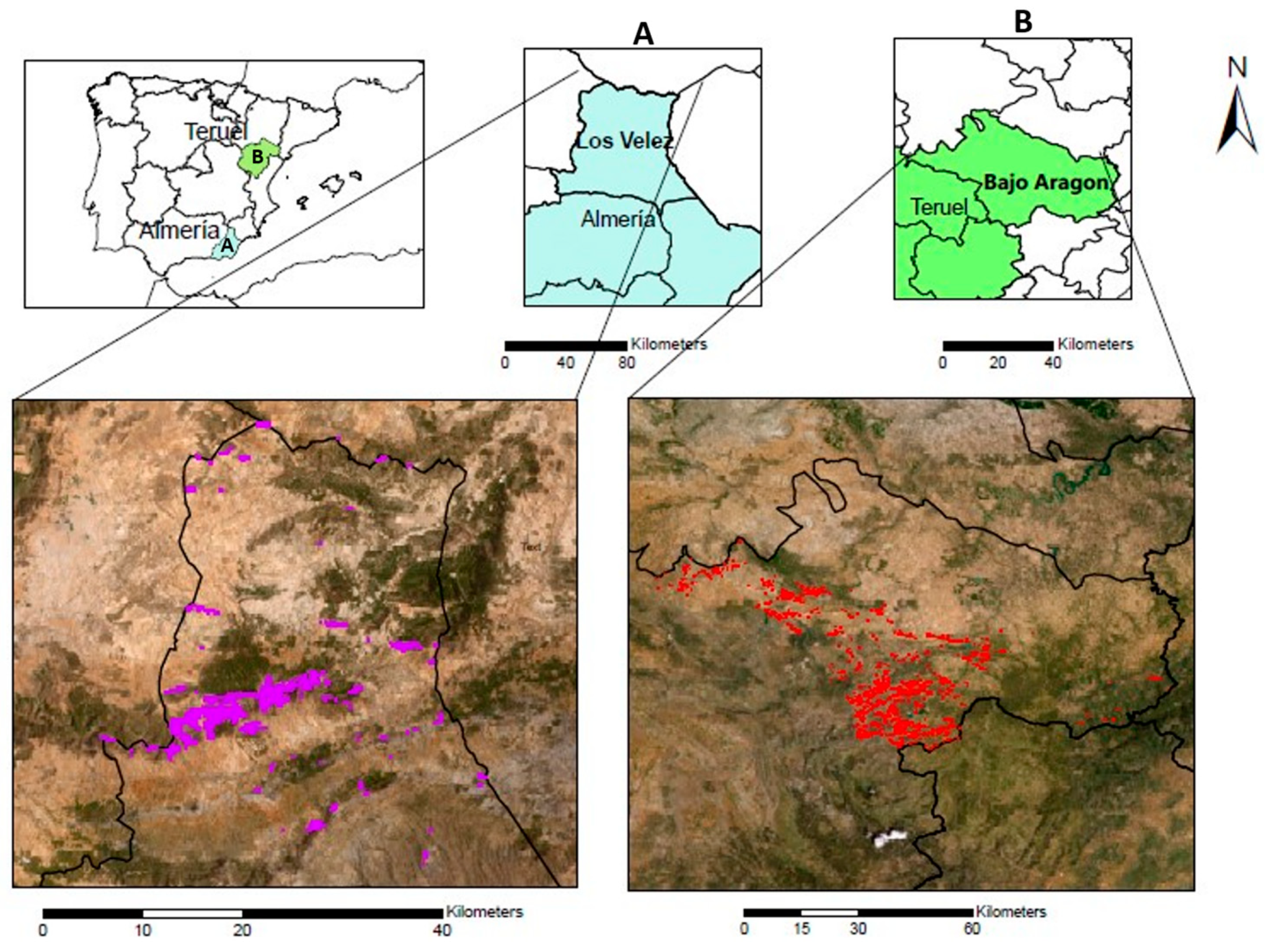
2.1. Area of Study

An extensive area of rangelands was selected in the agricultural region of Los Velez, in Almeria province, southeast of Spain (Figure 1A). This region presents a mountainous landscape with a slope from 1% to 14%, with regosols (Xerochrept) soils formed on limestones and dolomites and a poorly developed horizons profile, finding a horizon C immediately above horizon A [40].

Los Vélez has a Mediterranean climate (Bsk, according to Köppen classification). It has average monthly temperatures ranging from 5.4 °C to 22.7 °C, and average yearly precipitations between 330 and 390 mm [41]. In this area, 47% of the surface is dedicated to crops, 31% is forestry, and 26% is scrub, pastures, and meadows. Brushlands Thymus sp. and Rosmarinus sp. coexist with almond trees and cereal crops [42]. The area is characterised by Brachypodietalia phoenicoidis grasses and its only alliance, Brachypodion phoenicoidis. These are the more xerophytic and Mediterranean communities of the Festuco-Brometea class.

Bajo Aragón, in Teruel Province, is in the transitional area between the Iberian System and the Ebro Valley (Figure 1B). The analysed pixels are mainly located in the southern part of the region above 800 m altitude, with complex relief and slopes between 5% and 30% [43]. In this area, 41% of the surface is dedicated to crops, 21% is forestry, and 38% is scrub, pastures, and meadows. In the scrub landscape, repopulated pine forests and xeric grasslands are present [44]. These grasses are dominated by creeping grasses and legumes, which offer a compact and homogeneous physiognomic appearance bellowing to the alliances described within the order Festuco-Poetalia ligulatae [45]. On dry soils, they correspond to the Festuco-Brometea class, where Bromus erectus, Brachypodium phoenicoides, Avenula pratensis, Anthyllis vulneraria, and Potentilla neumanniana, among others, are characteristic.

The soils are cambisols (Calciorthid) and regosols (Xerochrept) formed on limestone and marl, with a more developed horizon profile: A-Bw-BC-C compared to Los Velez [46]. Bajo Aragón has a Mediterranean climate (Bsk, to Csa according to Köppen classification) with average monthly temperatures between 0.8 °C and 29.8 °C and annual rainfall between 350 and 600 mm [47].

2.2. Data Collection

Tragsatec provided the rangeland pixel selection in collaboration with Entidad Nacional de Seguros Agrarios (ENESA). Tragsatec used the “Sistema de Información Geográfico de Parcelas Agrícolas” (SIGPAC) from “Fondo Español De Garantía Agraria”, and the “Mapa Forestal Español” (MFE) [48]. Finally, 621 and 1952 pixels defined the Los Vélez and Bajo Aragón areas, respectively. The NDVI was extracted from the product MOD09GQ of the TERRA satellite and MYD09GQ of the AQUA satellite, which provide the reflectance of the red and near-infrared bands with which the index was built. NDVI series from 2002 to 2019 for each pixel, with a temporal resolution of 10 days (10-days composite period) and a spatial resolution of 250 m, were used in this study.

Shortwave infrared reflectance (SWIR, 2105–2155 nm) was collected from MOD09Q1.006 band 7 product from AppEEARS to calculate the Shortwave Transformed Reflectance (STR) [49]. This product has a 500 m spatial resolution, lower than the one used for the vegetation indices, but a higher spatial resolution was not available for this reflectance band. This band’s temporal resolution is 8 days (8-days composite period). SWIR series started from 2002 to 2019 to match the time series of NDVI corresponding to the pixel selection.

Daily meteorological data from the closest meteorological stations were also used [50]. Average temperature and accumulated precipitation were calculated every 10 days to match the NDVI dates.

2.3. Estimation of Vegetation and Soil Moisture Content Indices

NDVI was used to calculate another vegetation index mainly used for vegetation drought detection, the Vegetation Condition Index (VCI) [51]. This index was calculated following Equation (1), where NDVI is each value of the time series and ${\mathrm{N}\mathrm{D}\mathrm{V}\mathrm{I}}_{\mathrm{m}\mathrm{i}\mathrm{n}}$ and ${\mathrm{N}\mathrm{D}\mathrm{V}\mathrm{I}}_{\mathrm{m}\mathrm{a}\mathrm{x}}$ are their multiyear minimum and maximum, respectively, for every 10 days:

$$\mathrm{V}\mathrm{C}\mathrm{I}={\displaystyle \frac{\mathrm{N}\mathrm{D}\mathrm{V}\mathrm{I}-{\mathrm{N}\mathrm{D}\mathrm{V}\mathrm{I}}_{\mathrm{m}\mathrm{i}\mathrm{n}}}{{\mathrm{N}\mathrm{D}\mathrm{V}\mathrm{I}}_{\mathrm{m}\mathrm{a}\mathrm{x}}-{\mathrm{N}\mathrm{D}\mathrm{V}\mathrm{I}}_{\mathrm{m}\mathrm{i}\mathrm{n}}}}$$

(1)

To estimate surface soil moisture, we used the Optimised TRapezoid Model [25]. It is based on the linear physical relationship between SM and Shortwave infrared Transformed Reflectance (STR) and is parameterised based on the pixel distribution within the STR-NDVI space. The first step in OPTRAM model requires the STR, which was calculated using Equation (2):

$$\mathrm{S}\mathrm{T}\mathrm{R}={\displaystyle \frac{{(1-\mathrm{S}\mathrm{W}\mathrm{I}\mathrm{R})}^2}{2·\mathrm{S}\mathrm{W}\mathrm{I}\mathrm{R}}}$$

(2)

SWIR reflectance has the advantage that it does not significantly change with ambient atmospheric conditions. This is especially important when the analysis must use a long time series of soil moisture. Firstly, we converted the 8-days time STR series to 10-days period series like with the NDVI and VCI. For every month with 4 values of this time series, every two values were averaged to obtain 3 instead of 4. When a month had 3 values, its values remained untouched. Secondly, to match the STR and NDVI spatially, every NDVI pixel was given an STR value based on its centroid proximity. Therefore, STR spatial resolution (500 m) was adapted to NDVI spatial resolution (250 m). After building a dataset of time series and pixels, this was made for every pixel in all its time series. We proceeded to calculate the trapezoidal space NDVI-STR (Figure 2). The pixels corresponding to wet soil are located on the upper edge of the trapezoid (wet edge), and the pixels corresponding to dry soil are located on the lower edge of the trapezoid (dry edge). The soil moisture component (W) is normalised using the local minimum dry and maximum wet soil moisture content, as presented in Equation (3):

$${\mathrm{W}}_{\mathrm{i}}={\displaystyle \frac{{\mathsf{\theta }}_{\mathrm{i}}-{\mathsf{\theta }}_{\mathrm{d}}}{{\mathsf{\theta }}_{\mathrm{w}}-{\mathsf{\theta }}_{\mathrm{d}}}}={\displaystyle \frac{{\mathrm{S}\mathrm{T}\mathrm{R}}_{\mathrm{i}}-{\mathrm{S}\mathrm{T}\mathrm{R}}_{{\mathrm{m}\mathrm{i}\mathrm{n}}_{\mathrm{i}}}}{{\mathrm{S}\mathrm{T}\mathrm{R}}_{{\mathrm{m}\mathrm{a}\mathrm{x}}_{\mathrm{i}}}-{\mathrm{S}\mathrm{T}\mathrm{R}}_{{\mathrm{m}\mathrm{i}\mathrm{n}}_{\mathrm{i}}}}}$$

(3)

where ${\mathsf{\theta }}_{\mathrm{i}}$ is the surface soil moisture at date i, ${\mathsf{\theta }}_{\mathrm{d}}$ is the local minimum dry soil moisture content, ${\mathsf{\theta }}_{\mathrm{w}}$ is the local maximum wet soil moisture content, ${\mathrm{S}\mathrm{T}\mathrm{R}}_{\mathrm{i}}$ is the transformed SWIR reflection coefficient at date i, ${\mathrm{S}\mathrm{T}\mathrm{R}}_{{\mathrm{m}\mathrm{i}\mathrm{n}}_{\mathrm{i}}}$ is the transformed reflectance of dry soil, and ${\mathrm{S}\mathrm{T}\mathrm{R}}_{{\mathrm{m}\mathrm{a}\mathrm{x}}_{\mathrm{i}}}$ is the transformed reflectance of wet soil. The dry and wet edges formed a theoretical trapezoid between the STR and NDVI space, and they are defined as Equation (4):

$$\begin{array}{c}{\mathrm{S}\mathrm{T}\mathrm{R}}_{{\mathrm{m}\mathrm{i}\mathrm{n}}_{\mathrm{i}}}={\mathrm{i}}_{\mathrm{d}}+{\mathrm{s}}_{\mathrm{d}}{\mathrm{N}\mathrm{D}\mathrm{V}\mathrm{I}}_{\mathrm{i}}\\ {\mathrm{S}\mathrm{T}\mathrm{R}}_{{\mathrm{m}\mathrm{a}\mathrm{x}}_{\mathrm{i}}}={\mathrm{i}}_{\mathrm{w}}+{\mathrm{s}}_{\mathrm{w}}{\mathrm{N}\mathrm{D}\mathrm{V}\mathrm{I}}_{\mathrm{i}}\end{array}$$

(4)

The parameters ${\mathrm{i}}_{\mathrm{d}}$ and ${\mathrm{s}}_{\mathrm{d}}$ are the intercept and the slope of the dry (upper) edge, and ${\mathrm{i}}_{\mathrm{w}}$ and ${\mathrm{s}}_{\mathrm{w}}$ are the intercept and the slope of the wet (lower) edge (Figure 2). Using these parameters, W is calculated using Equation (5):

$${\mathrm{W}}_{\mathrm{i}}={\displaystyle \frac{{\mathrm{S}\mathrm{T}\mathrm{R}}_{\mathrm{i}}-{\mathrm{i}}_{\mathrm{d}}-{\mathrm{s}}_{\mathrm{d}}{\mathrm{N}\mathrm{D}\mathrm{V}\mathrm{I}}_{\mathrm{i}}}{{\mathrm{i}}_{\mathrm{d}\mathrm{w}}-{\mathrm{i}}_{\mathrm{d}}+{(\mathrm{s}}_{\mathrm{w}}-{\mathrm{s}}_{\mathrm{d}}){\mathrm{N}\mathrm{D}\mathrm{V}\mathrm{I}}_{\mathrm{i}}}}$$

(5)

Note that W depends on STR and ultimately from SWIR. NDVI is only a scale factor to determine ${\mathrm{S}\mathrm{T}\mathrm{R}}_{{\mathrm{m}\mathrm{i}\mathrm{n}}_{\mathrm{i}}}$ and ${\mathrm{S}\mathrm{T}\mathrm{R}}_{{\mathrm{m}\mathrm{a}\mathrm{x}}_{\mathrm{i}}}$. Even though there is a linear relationship between STR and W (Equation (3)), this is not found between NDVI and W, as the dry and wet edges are not parallel lines (Figure 2). A time-lagged cross-correlation analysis was performed to check that W estimation does not impose a significant relation with NDVI that could bias the estimation of the probabilities applied in this work.

We took another step in calculating the Water Condition Index (WCI), submitting the W to the same transformation NDVI had undergone to calculate VCI. Therefore, we calculated the WCI using Equation (6):

$$\mathrm{W}\mathrm{C}\mathrm{I}={\displaystyle \frac{\mathrm{W}-{\mathrm{W}}_{\mathrm{m}\mathrm{i}\mathrm{n}}}{{\mathrm{W}}_{\mathrm{m}\mathrm{a}\mathrm{x}}-{\mathrm{W}}_{\mathrm{m}\mathrm{i}\mathrm{n}}}}$$

(6)

where W is each value of the time series and ${\mathrm{W}}_{\mathrm{m}\mathrm{i}\mathrm{n}}$ and ${\mathrm{W}}_{\mathrm{m}\mathrm{a}\mathrm{x}}$ are, respectively, their multiyear minimum and maximum for every 10 days.

For both WCI and VCI, anomaly values were calculated using a Z-score per each date of the year (standardisation) as in Equation (7):

$$\begin{array}{c}{Z}_{WCI}={\displaystyle \frac{\mathrm{W}\mathrm{C}\mathrm{I}-{\mathsf{\mu }}_{\mathrm{W}\mathrm{C}\mathrm{I}}}{{\mathsf{\sigma }}_{\mathrm{W}\mathrm{C}\mathrm{I}}}}\\ Z_{VCI}={\displaystyle \frac{\mathrm{V}\mathrm{C}\mathrm{I}-{\mathsf{\mu }}_{\mathrm{V}\mathrm{C}\mathrm{I}}}{{\mathsf{\sigma }}_{\mathrm{V}\mathrm{C}\mathrm{I}}}}\end{array}$$

(7)

where μ is the yearly average and σ is the yearly standard deviation for each year’s date. Any trend or seasonal variation is removed with a Z-score formula, highlighting only the anomaly events.

2.4. Estimation of Probabilities of WCI and VCI Anomalies

The probabilities of surpassing different thresholds were calculated for WCI anomalies ($Z_{WCI}$) and VCI anomalies ($Z_{VCI}$) every 10 days throughout the time series. Three thresholds (−0.5, −0.7, and −1) were selected following the thresholds used for Standard Precipitation Index (SPI) [17] and Standard Precipitation Evaporation Index (SPEI) [52], indices commonly used for drought monitoring [53,54]. These thresholds were established based on previous research for drought identification using the multi-thresholds run theory [55,56].

Firstly, we calculated an estimation of the probability of negative $Z_{VCI}$ and negative $Z_{WCI}$ at period i (every 10 days) for the given time series using Equation (8):

$$\begin{array}{c}P(Z_{VCI}<“\mathrm{th}” \mathrm{a}\mathrm{t} \mathrm{t}\mathrm{h}\mathrm{e} \mathrm{p}\mathrm{e}\mathrm{r}\mathrm{i}\mathrm{o}\mathrm{d} \mathrm{i} )\\ P(Z_{WCI}<“\mathrm{th}” \mathrm{a}\mathrm{t} \mathrm{t}\mathrm{h}\mathrm{e} \mathrm{p}\mathrm{e}\mathrm{r}\mathrm{i}\mathrm{o}\mathrm{d} \mathrm{i})\end{array}$$

(8)

where $\mathrm{“}\mathrm{t}\mathrm{h}\mathrm{”}$ are the three different thresholds: −0.5, −0.7, and −1.0. For easier understanding, this will be called “base probability”.

Secondly, an estimation of the conditional probability going through each threshold of the $Z_{VCI}$ at the period i given a $Z_{WCI}$ below −0.3 at the same period i was also calculated using Equation (9):

$$P\left(Z_{VCI}<“\mathrm{t}\mathrm{h}\mathrm{”} \mathrm{a}\mathrm{t} \mathrm{t}\mathrm{h}\mathrm{e} \mathrm{p}\mathrm{e}\mathrm{r}\mathrm{i}\mathrm{o}\mathrm{d} \mathrm{i} \right| Z_{WCI}<-0.3 \mathrm{a}\mathrm{t} \mathrm{t}\mathrm{h}\mathrm{e} \mathrm{s}\mathrm{a}\mathrm{m}\mathrm{e} \mathrm{p}\mathrm{e}\mathrm{r}\mathrm{i}\mathrm{o}\mathrm{d} \mathrm{i})$$

(9)

where $\mathrm{“}\mathrm{t}\mathrm{h}\mathrm{”}$ are the three different thresholds: −0.5, −0.7, and −1.0. This probability measures the correlation between SM and vegetation anomaly occurrences at the same period. This probability will be called as “lag-0 conditional probability”.

Finally, an estimation of the conditional probability going through each threshold of the $Z_{VCI}$ at the period i given a $Z_{WCI}$ below −0.3 four periods (lags) before was calculated using Equation (10):

$$\begin{array}{c}P\left(Z_{VCI}<\mathrm{“}\mathrm{t}\mathrm{h}\mathrm{”} \mathrm{a}\mathrm{t} \mathrm{t}\mathrm{h}\mathrm{e} \mathrm{p}\mathrm{e}\mathrm{r}\mathrm{i}\mathrm{o}\mathrm{d} \mathrm{i} \right| Z_{WCI}\\ <-0.3 \mathrm{a}\mathrm{t} \mathrm{t}\mathrm{h}\mathrm{e} \mathrm{p}\mathrm{e}\mathrm{r}\mathrm{i}\mathrm{o}\mathrm{d} \mathrm{i} \mathrm{m}\mathrm{i}\mathrm{n}\mathrm{u}\mathrm{s} 4 \mathrm{p}\mathrm{e}\mathrm{r}\mathrm{i}\mathrm{o}\mathrm{d}\mathrm{s} \mathrm{o}\mathrm{r} \mathrm{l}\mathrm{a}\mathrm{g}\mathrm{s})\end{array}$$

(10)

where $\mathrm{“}\mathrm{t}\mathrm{h}\mathrm{”}$ are the three different thresholds: −0.5, −0.7, and −1.0. This probability measures the correlation between both anomalies with 4 lags of delay. This probability will be named as “lag-4 conditional probability”.

The percentual relative frequency was used for the estimation of both types of probability and, for clarity, percentual frequency notation (0–100%) will be used instead of probabilities notation (0–1).

3. Results

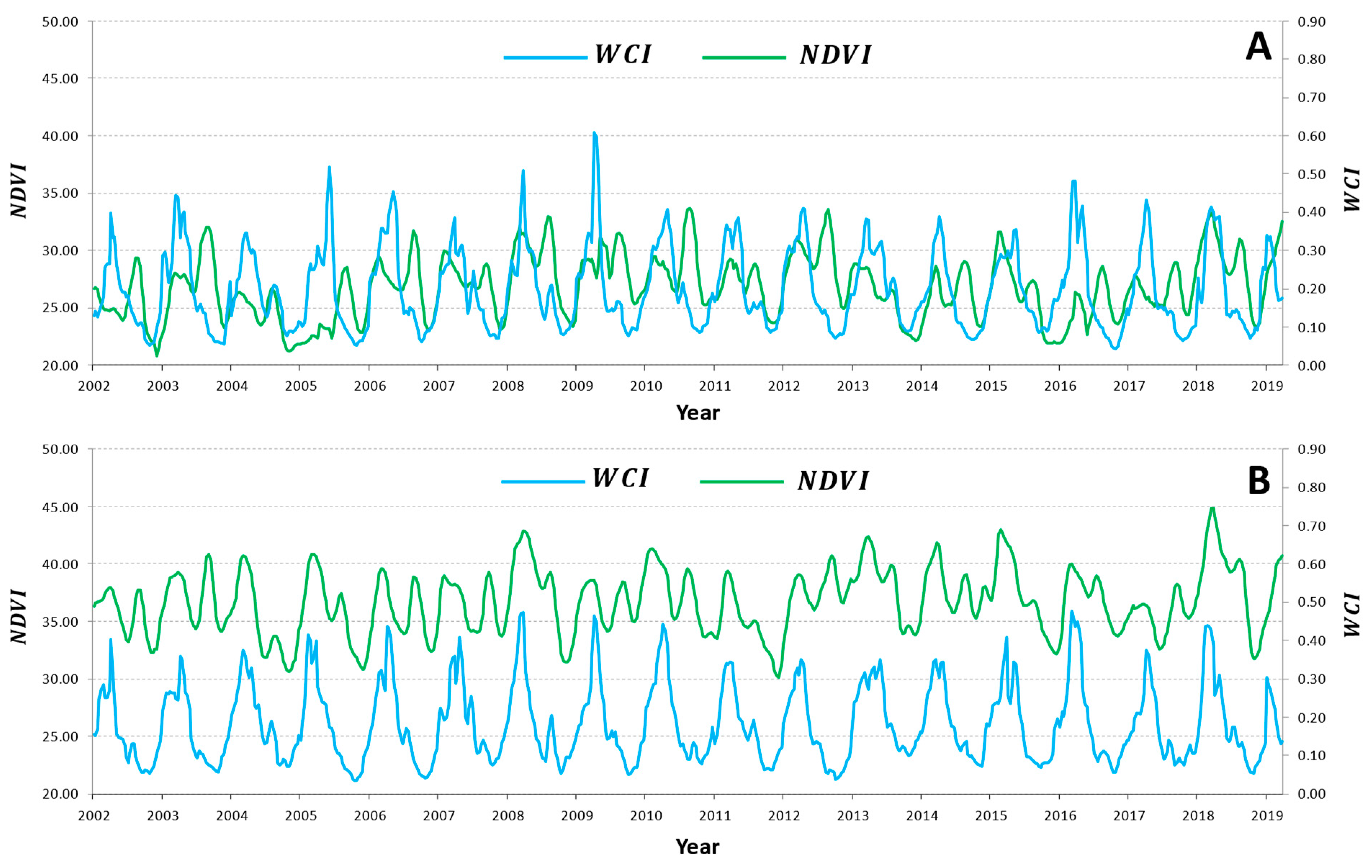
3.1. Soil Moisture and Vegetation Indices

The NDVI and WCI series obtained in each place are shown in Figure 3. Both areas show a different range of values, particularly in NDVI, as expected due to the different characteristics described in Section 2.1.

Los Velez’s NDVI series values range from 22 to 33. Meanwhile, those of Bajo Aragón range from 32 to 45. Therefore, these values show the semiarid conditions in both areas. Concerning their annual pattern, visual inspection points out differences that will be quantified in the VCI series.

WCI series shows similarity in the range of values. Los Velez’s WCI series range from 0.04 to 0.61, and those of Bajo Aragón range from 0.04 to 0.48. The WCI annual pattern in Los Velez is similar to that in Bajo Aragón.

Cross-correlation analysis (Figure 4) shows a significant correlation between WCI and NDVI at the lags (from 0 to 4) used to estimate conditional probabilities.

3.2. Water and Vegetation Condition Indices

Firstly, we studied the dynamics of VCI and WCI for Los Velez (Almería province) and Bajo Aragón (Teruel province). Figure 5A shows the dynamic of the VCI for Loz Vélez (green box plots). The vegetation activity, measured by VCI, increases from the end of summer until the middle of November, then decreases until the middle of March and increases again until the end of May. Therefore, VCI dynamics do not match the seasons: a rise and a drop are observed during autumn, spring, and summer, while VCI dynamics match better during winter. Figure 5A also shows the behaviour of the SM content, measured by WCI (red box plots), during a year. The evolution of both indices is very similar from the end of August to the middle of March. However, from March to the end of May, WCI suffers a continuous downfall, unlike the VCI, which increases in this period.

Figure 5B shows the dynamic of the VCI for Bajo Aragón (green box plots). In this case, VCI also increases during the end of summer but extends to the beginning of December, then decreases until the middle of March and increases again until the beginning of June. For this area, VCI dynamics match better the seasons autumn, winter, and spring, while a rise and a drop are observed during summer. Figure 5B also shows the dynamic of WCI (red box plots) during a year. The evolution of both indices is very similar from the middle of August to the middle of March. By contrast, from April to the beginning of June, WCI suffers a continuous downfall, unlike the VCI that goes up in this period, with similar behaviour to Los Vélez.

Following [57], four phases were proposed to analyse the vegetation and SM content dynamics. The criterion used to delimit the phases was the slope change in the VCI median. For Los Vélez, VCI and WCI have more similar dynamics in phases 1, 2, and 4. In phase 1, VCI increases due to vegetation activation after the summer. WCI also rises due to the effect of moisture increments in the soil due to the beginning of rainfall. The maximum VCI activity occurs at the end of phase 1 (the middle of November), while WCI peaks during the middle of phase 2 (the end of January). The low temperatures in phase 2 (see Figure 6A) cause a reduction in plant activity and a continuous decrease in the VCI graph during this phase. When phase 3 begins, the temperature increases and the WCI graph decreases. This pattern occurs because the most superficial layers of the soil are losing moisture. In phase 3, precipitations are present (see Figure 6A), but temperature and evapotranspiration play an essential role in superficial soil water content, obscuring the relationship between precipitation and SM content [57,58]. The VCI graph has another peak at the end of phase 3 because of photosynthetic activity growth. In phase 4, both graphs decrease because of high temperatures and low precipitation during this period of the year.

For Bajo Aragón, VCI and WCI have dynamics similar to those in phases 1, 2, and 4, as in Los Vélez. In phase 1, VCI and WCI increase due to vegetation activation and abundant precipitations (see Figure 6B). The maximum VCI activity (the end of phase 1) is delayed for two 10-day periods compared to Los Vélez. In contrast, the maximum WCI at the beginning of phase 2 is advanced four 10-day periods compared to Los Vélez. It should be noted that phase 1 in Bajo Aragón is more prolonged than in Los Vélez. Conversely, phase 2 in Los Vélez is longer than in Bajo Aragón. Phases 3 and 4 in Bajo Aragón are similar to those in Los Vélez, with the same duration and time limits. The only difference is that, in phase 3, the VCI maximum in Los Vélez is higher than in Bajo Aragón, probably due to the vegetation of the area had a better condition to grow because of high and prolonged precipitation in phase 2 (see Figure 6A).

Secondly, we studied the series of anomaly indices, $Z_{VCI}$ and $Z_{WCI}$, averaged over the two studied areas. In both plots of Figure 7, it can be observed that $Z_{VCI}$ series are usually smoother than $Z_{WCI}$ series, which present a rougher profile with higher peaks. This behaviour reveals that the vegetation response to environmental changes is slower than the soil moisture response. In Figure 7A, $Z_{VCI}$ serie reflects the long periods of intense drought suffered in Los Vélez the years 2004–2005, 2013–2014, and 2015–2016, when $Z_{VCI}$ reached very low values, approximately −2.0. The drought periods in Bajo Aragón occurred in 2004, 2011–2012, and 2017 (Figure 7B).

For Los Vélez (Figure 8A), the probability of $Z_{VCI}$ to be below the first threshold (−0.5) is high in two main periods: the first during the end of January and the whole of February (with 35%), and the second during April and the beginning of May (with 40–45%). For the threshold −0.7, the periods of high probability are similar to those of the −0.5 threshold, although the probability values are lower than those obtained with the other threshold. On the other hand, the probability for $Z_{VCI}$ to be below −1.0 is kept relatively constant most of the year, increasing approximately from 10% to 25% from September to October.

For Bajo Aragón (Figure 8B), the probability for $Z_{VCI}$ to be below the thresholds −0.5 and −0.7 is relatively constant most of the year, although the probability values for the threshold −0.7 are always lower than −0.5, especially in March. The probability for $Z_{VCI}$ to surpass below −1.0 is especially low from December to March, when the values are approximately between 5% and 10%.

A similar graphic, but for $Z_{WCI}$, is presented in Figure 9. In Los Vélez (Figure 9A), the base probabilities for the thresholds −0.5 and −0.7 show a similar pattern. In both thresholds, the base probabilities are high for two main periods: the first from January to February, and the second in June. For the threshold −0.5, the base probability in these two periods is 35–40%. It can be observed that the base probability for the threshold −1.0 shows more periods with 0% compared to $Z_{VCI}$.

In Bajo Aragón (Figure 9B), the base probability for the threshold −0.5 is especially high in October (45%), while for the threshold −0.7 it is not observed during any outstanding period. However, for the probability of surpassing below the threshold −1.0, we find that this is especially low in March, with values of 5%.

In addition to this, the probabilities of $Z_{WCI}$ and $Z_{WCI}$ for the different thresholds can be compared with expected probabilities on standardised data. If the indices, $Z_{WCI}$ and $Z_{WCI}$, followed normal distributions, the probabilities would be $P(Index<-0.5)=0.309$, $P(Index<-0.7)=0.242$, and $P(Index<-1.0)=0.159$, which is not the case for the majority for the 10-day periods.

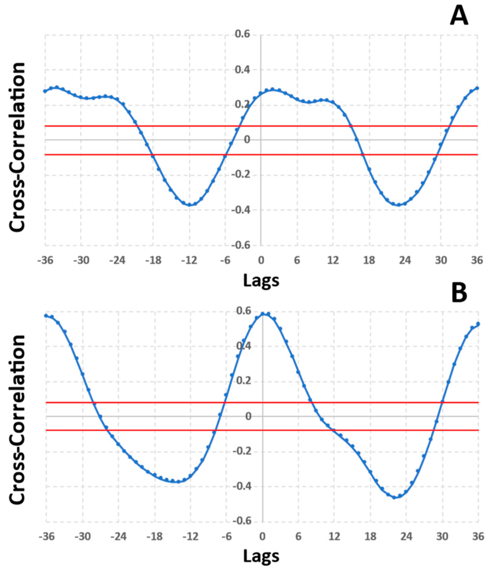
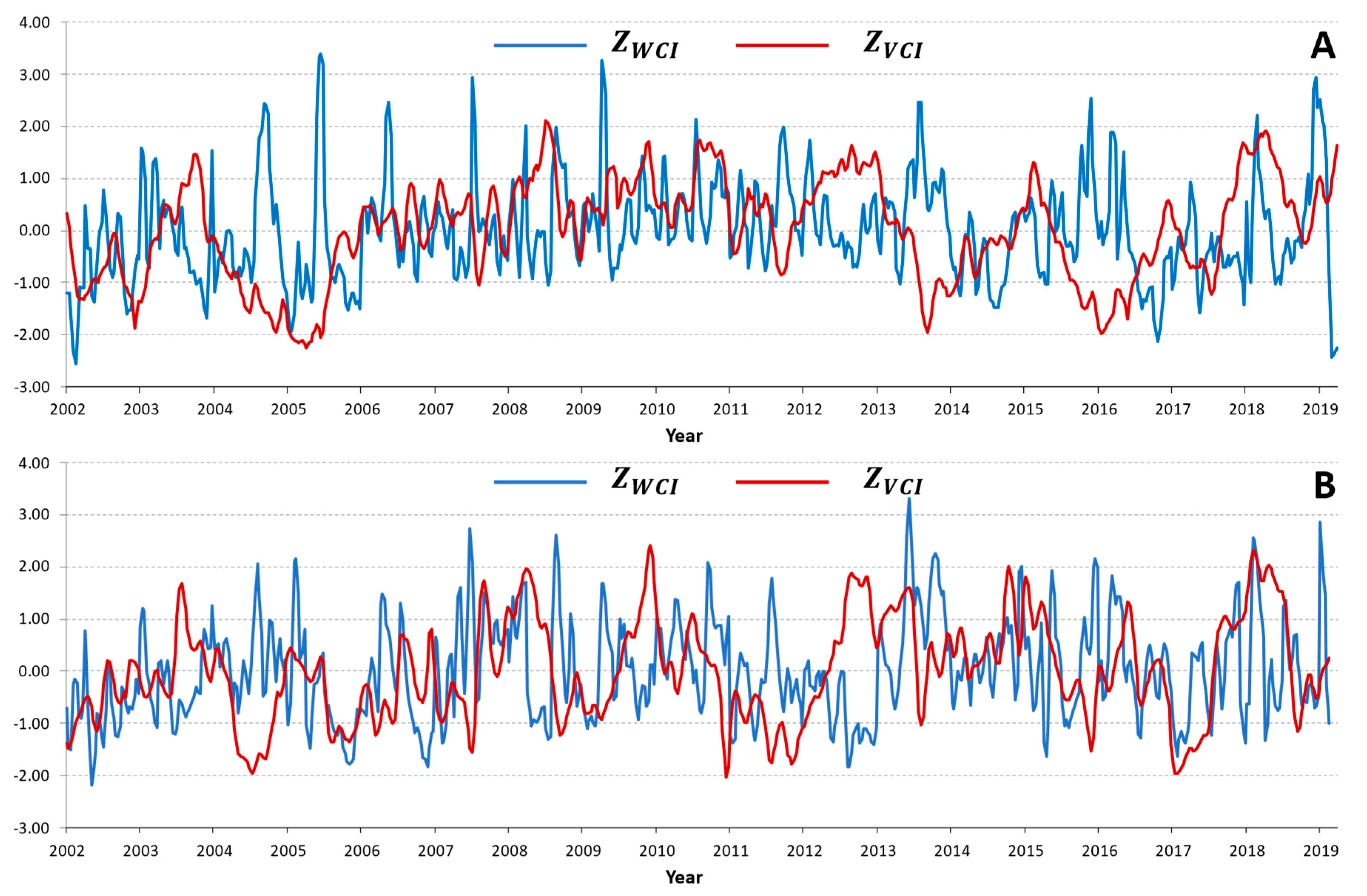
3.3. Relationship of VCI and WCI Anomalies

For each threshold (−0.5, −0.7, and −1.0), the base probability of $Z_{VCI}$ and two conditional probabilities (lag-0 and lag-4) are shown in Figure 10, Figure 11 and Figure 12.

In Los Vélez, for all thresholds (Figure 10A, Figure 11A and Figure 12A), the lag-0 conditional probability is higher than the base probabilities from September to April. Moreover, the lag-4 conditional probability is higher than the 0-lag conditional probability from the middle of November to April, except for February for the threshold of −0.5 and December for the threshold of −1.0. Los Vélez shows high values in the lag-4 conditional probability with minor anomalies (−0.5 and −0.7), often reaching from 50% to 65% of probability from November to January (compared to an average of 20–30% of base probability). These probabilities decrease when threshold −1.0 is used, reaching a maximum of 50% in the middle of January. Although the lag-4 conditional probabilities are low for the threshold −1.0, they remain above the base probability from October to April.

In Bajo Aragón (Figure 10, Figure 11B and Figure 12B), the periods where the lag-0 conditional probability is higher than the base probability are not so well-defined as those in Los Vélez. In fact, unlike in Los Velez, we find all the summers with lag-0 conditional probability higher than the base probability for all the thresholds. Regarding lag-4 conditional probability, we find a long period where the one is higher than the base probability for all the thresholds. This period occurs from September to the beginning of February, with probability values reaching 60–70%, approximately, during December and January, with smaller thresholds (−0.5 and −0.7). For the rest of the year, we can observe some short alternating periods where the lag-4 conditional probability is higher than the base probability, i.e., in May and August for the threshold of −0.5 and March and August for the threshold of −0.7.

4. Discussion

Figure 13 shows a comparison, for both areas, of the positive difference between the lag-4 conditional probability and the base probability every 10 days of the year and for the three different thresholds (A, B, and C). This Figure summarises the periods where the knowledge of $Z_{WCI}$ increases the predictability of $Z_{VCI}$ four lags later compared to the base probability.

In Los Vélez, the lag-4 conditional probability is higher than the base probability from October to April for all thresholds. On the contrary, in Bajo Aragón, this occurs from the middle of July to the beginning of February. Therefore, we find two long periods where the capability of predicting VCI anomalies could be increased in both areas. In Bajo Aragón, this increase in prediction starts before, probably due to higher precipitation in June and July than in Los Vélez.

For Los Vélez, the increment in predictability from the middle of November to the beginning of February is evident when we consider low anomalies of VCI, i.e., for the thresholds −0.5 and −0.7. The increment in these months reaches 25–35% in November and December. On the other hand, the values range from 10% to 20% during March and April. When we consider high anomalies of VCI, i.e., for the threshold −1.0, the predictability decreases in all months, with values in the range from 5% to 20%. It should be noted that the middle of January shows higher predictability values, over 30%, than the other thresholds.

In Bajo Aragón, we find higher positive differences in the same period than In Los Vélez, i.e., from the middle of November to the beginning of February for the thresholds −0.5 and −0.7. The increment in these months reaches 30–35% in January and the beginning of February. By contrast, in Bajo Aragón, we find intermittent periods of high predictability values during March (10–15%) and May (10–30%). The more outstanding difference between both areas is the presence of higher predictability at the end of July, August, and September. In these periods, we have zero increase in predictability in Los Velez but a 5–15% increase in Bajo Aragón. These values of positive differences persist in August and September, even in the case of high anomalies of VCI, for the threshold of −1.0.

From October to January, precipitation is more or less abundant in both areas but is consistent with low temperatures. Therefore, this could explain why the predictability of vegetation anomalies using the SM content index is improved from November to the beginning of February. When precipitation continues to fall, but temperatures begin to rise, from February to the end of April, the predictability starts to decrease due to temperature and evapotranspiration playing a major role in SM content [57,58,59]. In Los Vélez, precipitation decreases strongly from May, and temperatures start to increase until the end of summer. In these periods, the SM content does not give extra information about anomalies in vegetation. By contrast, in Bajo Aragón, we find relatively high precipitation until June and more precipitation than Los Vélez in July and August. This scenario could explain why we have increments in predictability during August and September in Bajo Aragón.

Early warning systems are being developed for famine, agricultural yield, and drought. Recently, remote sensing has been used in this regard and is more commonly used for rangeland monitoring. In this work, we merged remote sensing vegetation monitoring with early warning indices, $Z_{WCI}$, to inform managers and rangers [60,61] and showed that early SM content anomalies can relevantly improve the predictability of vegetation condition anomalies in some specific months.

5. Conclusions

SM content and vegetation indices show more similar dynamics in the months with lower temperatures in both study areas, from autumn to the beginning of spring. In these months, given the low temperatures, precipitation leads to vegetation growth. In the later months, when the temperature rises, SM availability depends mainly on evapotranspiration and vegetation type.

The stronger relationship between precipitation and vegetation from autumn to the beginning of spring is reflected in the feasibility of $Z_{WCI}$ to aid the prediction of vegetation anomalies $Z_{VCI}$. During these months, using $Z_{WCI}$ as a warning index is possible for Los Velez and Bajo Aragón. Both are considered semiarid rangelands.

Lag-4 conditional probability measures the probability of an anomaly of VCI occurring when an anomaly of WCI has already happened four periods (10 days) before. When we compared this probability with the base probability (the probability of an anomaly of VCI), we detected some periods of the year where the knowledge of an anomaly of SM content allowed us to increase the probability of the occurrence of an anomaly of vegetation.

The two study areas showed an increase of 10–35% in the predictability of vegetation index anomalies $Z_{VCI}$ (thresholds −0.5 and −0.7) from November to the beginning of February. Additionally, in Bajo Aragón, we also find an increase in the capability of prediction from July to September due to more precipitation and lower temperatures in June compared with Los Vélez. Therefore, we could increase the predictability of anomalies of VCI in some specific periods if we detect anomalies in the WCI four 10-day periods before.

$Z_{VCI}$ is one of the indices used to monitor vegetation growth anomalies. Additional monitoring of the $Z_{WCI}$ index allows predicting VCI anomaly events in advance and farmers to make early decisions about their rangelands.

This study presents several limitations, some due to remote sensing techniques and others due to the limits of the areas of study. Temporal lengths and pixel resolution are limited by satellite data availability, a common problem in remote sensing. Exploring new satellite data with better temporal and spatial resolution could help to improve and strengthen the conclusions of this study. Further research is needed to expand to other areas, vegetations, and ecoregions, using different soil moisture approaches and more climatic variables to understand vegetation dynamics.

References

1. Adegoke, J.O.; Carleton, A.M. Relations between Soil Moisture and Satellite Vegetation Indices in the U.S. Corn Belt. J. Hydrometeorol. 2002, 3, 395–405. [Google Scholar] [CrossRef]
2. Felegari, S.; Sharifi, A.; Moravej, K.; Golchin, A.; Tariq, A. Investigation of the relationship between ndvi index, soil moisture, and precipitation data using satellite images. In Sustainable Agriculture Systems and Technologies; Wiley Online Library: Hoboken, NJ, USA, 2022; pp. 314–325. [Google Scholar] [CrossRef]
3. Sharma, M.; Bangotra, P.; Gautam, A.S.; Gautam, S. Sensitivity of normalised difference vegetation index (NDVI) to land surface temperature, soil moisture and precipitation over district Gautam Buddh Nagar, UP, India. Stoch. Environ. Res. Risk Assess. 2022, 36, 1779–1789. [Google Scholar] [CrossRef] [PubMed]
4. Hirschi, M.; Mueller, B.; Dorigo, W.; Seneviratne, S.I. Using remotely sensed soil moisture for land-atmosphere coupling diagnostics: The role of surface vs. root-zone soil moisture variability. Remote Sens. Environ. 2014, 154, 246–252. [Google Scholar] [CrossRef]
5. Albergel, C.; Udiger, C.R.; Pellarin, T.; Calvet, J.-C.; Fritz, N.; Froissard, F.; Suquia, D.; Petitpa, A.; Piguet, B.; Martin, E. Hydrology and Earth System Sciences From near-surface to root-zone soil moisture using an exponential filter: An assessment of the method based on in-situ observations and model simulations. Hydrol. Earth Syst. Sci. 2008, 12, 1323–1337. [Google Scholar] [CrossRef]
6. Babaeian, E.; Sadeghi, M.; Jones, S.B.; Montzka, C.; Vereecken, H.; Tuller, M. Ground, proximal, and satellite remote sensing of soil moisture. Rev. Geophys. 2019, 57, 530–616. [Google Scholar] [CrossRef]
7. Liu, W.T.; Kogan, F.N. Monitoring regional drought using the vegetation condition index. Int. J. Remote Sens. 1996, 17, 2761–2782. [Google Scholar] [CrossRef]
8. Wang, X.; Xie, H.; Guan, H.; Zhou, X. Different responses of MODIS-derived NDVI to root-zone soil moisture in semi-arid and humid regions. J. Hydrol. 2007, 340, 12–24. [Google Scholar] [CrossRef]
9. Guan, Y.; Lu, H.; Yin, C.; Xue, Y.; Jiang, Y.; Kang, Y.; He, L.; Heiskanen, J. Vegetation response to climate zone dynamics and its impacts on surface soil water content and albedo in China. Sci. Total. Environ. 2020, 747, 141537. [Google Scholar] [CrossRef]
10. Schnur, M.T.; Xie, H.; Wang, X. Estimating root zone soil moisture at distant sites using MODIS NDVI and EVI in a semi-arid region of southwestern USA. Ecol. Inform. 2010, 5, 400–409. [Google Scholar] [CrossRef]
11. Allaby, M. Droughts; Infobase Publishing: New York, NY, USA, 2014. [Google Scholar]
12. American Meteorological Society: Meteorological drought—Policy statement. Bull. Am. Meteorol. Soc. 1997, 78, 847–849.
13. American Meteorological Society: AMS statement on meteorological drought. Bull. Am. Meteorol. Soc. 2004, 85, 771–773.
14. Wilhite, D.A.; Buchanan-Smith, M. Drought as hazard: Understanding the natural and social context. Drought Water Cris. Sci. Technol. Manag. Issues 2005, 3, 29. [Google Scholar]
15. Kim, D.-W.; Byun, H.-R.; Choi, K.-S. Evaluation, modification, and application of the Effective Drought Index to 200-Year drought climatology of Seoul, Korea. J. Hydrol. 2009, 378, 1–12. [Google Scholar] [CrossRef]
16. Mahmoudi, P.; Rigi, A.; Kamak, M.M. Evaluating the sensitivity of precipitation-based drought indices to different lengths of record. J. Hydrol. 2019, 579, 124181. [Google Scholar] [CrossRef]
17. McKee, T.B.; Doesken, N.J.; Kleist, J. The relationship of drought frequency and duration to time scales. In Proceedings of the 8th Conference on Applied Climatology, Anaheim, CA, USA, 17–22 January 1993; Volume 17, pp. 179–183. [Google Scholar]
18. Byun, H.-R.; Wilhite, D.A. Objective quantification of drought severity and duration. J. Clim. 1999, 12, 2747–2756. [Google Scholar] [CrossRef]
19. Willeke, G.; Hosking, J.R.M.; Wallis, J.R.; Guttman, N.B. The national drought atlas. Inst. Water Resour. Rep. 1994, 94. [Google Scholar]
20. AghaKouchak, A.; Farahmand, A.; Melton, F.S.; Teixeira, J.; Anderson, M.C.; Wardlow, B.D.; Hain, C.R. Remote sensing of drought: Progress, challenges and opportunities. Rev. Geophys. 2015, 53, 452–480. [Google Scholar] [CrossRef]
21. Wang, L.; Qu, J.J. Satellite remote sensing applications for surface soil moisture monitoring: A review. Front. Earth Sci. China 2009, 3, 237–247. [Google Scholar] [CrossRef]
22. Hao, Z.; AghaKouchak, A. Multivariate standardised drought index: A parametric multi-index model. Ad. Water Resour. 2013, 57, 12–18. [Google Scholar] [CrossRef]
23. Sheffield, J.; Goteti, G.; Wen, F.; Wood, E.F. A simulated soil moisture based drought analysis for the United States. J. Geophys. Res. Atmos. 2004, 109. [Google Scholar] [CrossRef]
24. Babaeian, E.; Sadeghi, M.; Franz, T.E.; Jones, S.; Tuller, M. Mapping soil moisture with the OPtical TRApezoid Model (OPTRAM) based on long-term MODIS observations. Remote. Sens. Environ. 2018, 211, 425–440. [Google Scholar] [CrossRef]
25. Sadeghi, M.; Babaeian, E.; Tuller, M.; Jones, S.B. The optical trapezoid model: A novel approach to remote sensing of soil moisture applied to Sentinel-2 and Landsat-8 observations. Remote. Sens. Environ. 2017, 198, 52–68. [Google Scholar] [CrossRef]
26. Chen, M.; Zhang, Y.; Yao, Y.; Lu, J.; Pu, X.; Hu, T.; Wang, P. Evaluation of the OPTRAM Model to Retrieve Soil Moisture in the Sanjiang Plain of Northeast China. Earth Space Sci. 2020, 7, e2020EA001108. [Google Scholar] [CrossRef]
27. Ambrosone, M.; Matese, A.; Di Gennaro, S.F.; Gioli, B.; Tudoroiu, M.; Genesio, L.; Miglietta, F.; Baronti, S.; Maienza, A.; Ungaro, F.; et al. Retrieving soil moisture in rainfed and irrigated fields using Sentinel-2 observations and a modified OPTRAM approach. Int. J. Appl. Earth Obs. Geoinf. 2020, 89, 102113. [Google Scholar] [CrossRef]
28. Ma, C.; Johansen, K.; McCabe, M.F. Combining Sentinel-2 data with an optical-trapezoid approach to infer within-field soil moisture variability and monitor agricultural production stages. Agric. Water Manag. 2022, 274, 107942. [Google Scholar] [CrossRef]
29. Skees, J.R.; Gober, S.; Varangis, P.; Lester, R.; Kalavakonda, V. Developing Rainfall-Based Index Insurance in Morocco; World Bank Publications: Washington, DC, USA, 2001; Volume 2577. [Google Scholar]
30. Wilhite, D. Drought Monitoring and Early Warning: Concepts, Progress and Future Challenges; World Meteorological Organization, WMO: Geneva, Switzerland, 2006. [Google Scholar]
31. Sepulcre-Canto, G.; Horion, S.; Singleton, A.; Carrao, H.; Vogt, J. Development of a Combined Drought Indicator to detect agricultural drought in Europe. Nat. Hazards Earth Syst. Sci. 2012, 12, 3519–3531. [Google Scholar] [CrossRef]
32. Jiménez-Donaire, M.d.P.; Tarquis, A.; Giráldez, J.V. Evaluation of a combined drought indicator and its potential for agricultural drought prediction in southern Spain. Nat. Hazards Earth Syst. Sci. 2020, 20, 21–33. [Google Scholar] [CrossRef]
33. Shofiyati, R.; Takeuchi, W.; Pasaribu, S.M.; Irawan, Y.R. Space-based drought analysis to support agricultural insurance facing climate change. IOP Conf. Ser. Earth Environ. Sci. 2021, 648, 012130. [Google Scholar] [CrossRef]
34. Canedo Rosso, C.; Hochrainer-Stigler, S.; Pflug, G.; Condori, B.; Berndtsson, R. Early warning and drought risk assessment for the Bolivian Altiplano agriculture using high resolution satellite imagery data. Nat. Hazards Earth Syst. Sci. Discuss. 2018, 2018, 1–23. [Google Scholar] [CrossRef]
35. Desai, B.; Maskrey, A.; Peduzzi, P.; de Bono, A.; Herold, C.; United Nations Office for Disaster Risk Reduction (UNISDR). Making Development Sustainable: The Future of Disaster Risk Management, Global Assessment Report on Disaster Risk Reduction; United Nations Office for Disaster Risk Reduction (UNISDR): Geneva, Switzerland, 2015. [Google Scholar]
36. Azhdari, Z.; Bazrafshan, O.; Shekari, M.; Zamani, H. Three-dimensional risk analysis of hydro-meteorological drought using multivariate nonlinear index. Theor. Appl. Clim. 2020, 142, 1311–1327. [Google Scholar] [CrossRef]
37. Hao, Y.; Hao, Z.; Fu, Y.; Feng, S.; Zhang, X.; Wu, X.; Hao, F. Probabilistic assessments of the impacts of compound dry and hot events on global vegetation during growing seasons. Environ. Res. Lett. 2021, 16, 074055. [Google Scholar] [CrossRef]
38. Ribeiro, A.F.S.; Russo, A.; Gouveia, C.M.; Páscoa, P.; Pires, C.A.L. Probabilistic modelling of the dependence between rainfed crops and drought hazard. Nat. Hazards Earth Syst. Sci. 2019, 19, 2795–2809. [Google Scholar] [CrossRef]
39. Sanz, E.; Martín-Sotoca, J.J.; Saa-Requejo, A.; Moratiel, R.; Almeida-Ñauñay, A.; Faraslis, I.; Tarquis, A.M. Temporal Coincidence of Soil Water and Vegetation Anomalies in Arid Rangelands. In Proceedings of the Estudios en la Zona No Saturada del Suelo VOL, Sevilla, Spanish, 7–9 November 2023; XVI. ZNS’23. pp. 109–114, ISBN 978-84-09-55828-5. [Google Scholar]
40. Aguilar Ruiz, J. Mapa de Suelos Escala 1:100 000. Provincia de Almería; Proyecto Lucdeme; Ministerio de Agricultura, Alimentación y Medio Ambiente (MAGRAMA): Madrid, Spain, 2004. [Google Scholar]
41. Grupo de Agroenergética de la E.T.S.I. Agrónomos (UPM). Caracterización de las Comarcas Agrarias de España; Tomo 6. Provincia de Almería; Ministerio de Agricultura, Alimentación y Medio Ambiente (MAGRAMA): Madrid, Spain, 2014. [Google Scholar]
42. Cueto, M.; Blanca, G. Flora del Parque Natural de Sierra María-Los Vélez; Sociedad Almeriense de Historia Natural: Almería, Spain, 1997. [Google Scholar]
43. Del Palacio Fernández-Montes, E.; Martín Fernández, L.; Hernández Álvarez, J.; Rojo Serrano, L. Inventario Nacional de Suelos. Teruel; Ministerio de Agricultura y Pesca, Alimentación y Medio Ambiente: Madrid, Spain, 2015; ISBN 978-84-491-1507-3. [Google Scholar]
44. Ibarra, P.; Nieto, V.; Echeverría, M.T.; Lozano, M.V.; Albero, M.J.; Julián, A.; Peña, J.L. La diversidad paisajística de Aragón. Utilidad de la cartografía de Paisaje a escala regional para el conocimiento, planificación y gestión del territorio. In Proceedings of the Actas del XXIII Congreso de Geógrafos Españoles AGE, Palma, Spanish, 23–25 October 2013; Espacios insulares y de frontera. Una visión geográfica. pp. 597–607. [Google Scholar]
45. San Miguel, A. Pastos Naturales Españoles. Caracterización, Aprovechamiento y Posibilidades de Mejora; Coedición Fundación Conde del Valle de Salazar- Mundi-Prensa: Madrid, Spain, 2001; 320p, ISBN 8471149915. [Google Scholar]
46. Ibarra Benlloch, P. La diversidad edáfica del territorio aragonés. In Geografía física de Aragón; Peña, J.L., Longares, L.A., Sánchez, M., Eds.; Universidad de Zaragoza: Zaragoza, Spain, 2004; pp. 41–53. ISBN 84-96214-29-X. [Google Scholar]
47. Grupo de Agroenergética de la E.T.S.I. Agrónomos (UPM). Caracterización de las Comarcas Agrarias de España; Tomo 45. Provincia de Teruel; Ministerio de Agricultura, Alimentación y Medio Ambiente (MAGRAMA): Madrid, Spain, 2014. [Google Scholar]
48. Fondo Español de Garantía Agraria (FEGA). Visor SIGPAC. Ministerio de Agricultura, Pesca y Alimentación. Gobierno de España. Available online: https://www.fega.gob.es/es/pepac-2023-2027/sistemas-gestion-y-control/sigpac (accessed on 20 June 2024).
49. Team, A. Application for Extracting and Exploring Analysis Ready Samples (AppEEARS); NASA EOSDIS Land Processes Distributed Active Archive Center (LP DAAC): Sioux Falls, SD, USA; USGS/Earth Resources Observation and Science (EROS) Center: Sioux Falls, SD, USA, 2020; Available online: https://Lpdaacsvc.Cr.Usgs.Gov/Appeears/ (accessed on 2 June 2020).
50. Sistema de Información Agroclimática para el Regadío (SIAR). Ministerio de Agricultura, Pesca y Alimentación. Gobierno de España. Available online: https://servicio.mapa.gob.es/websiar/Inicio.aspx (accessed on 20 June 2024).
51. Kogan, F. Application of vegetation index and brightness temperature for drought detection. Adv. Space Res. 1995, 15, 91–100. [Google Scholar] [CrossRef]
52. Vicente-Serrano, S.M.; Beguería, S.; López-Moreno, J.I. A multiscalar drought index sensitive to global warming: The standardised precipitation evapotranspiration index. J. Clim. 2010, 23, 1696–1718. [Google Scholar] [CrossRef]
53. Almeida-Ñauñay, A.F.; Villeta, M.; Quemada, M.; Tarquis, A.M. Assessment of Drought Indexes on Different Time Scales: A Case in Semiarid Mediterranean Grasslands. Remote. Sens. 2022, 14, 565. [Google Scholar] [CrossRef]
54. Pei, Z.; Fang, S.; Wang, L.; Yang, W. Comparative analysis of drought indicated by the SPI and SPEI at various timescales in inner Mongolia, China. Water 2020, 12, 1925. [Google Scholar] [CrossRef]
55. He, J.; Yang, X.; Li, Z.; Zhang, X.; Tang, Q. Spatiotemporal variations of meteorological droughts in China during 1961–2014: An investigation based on multi-threshold identification. Int. J. Disaster Risk Sci. 2016, 7, 63–76. [Google Scholar] [CrossRef]
56. Ma, Q.; Li, Y.; Liu, F.; Feng, H.; Biswas, A.; Zhang, Q. SPEI and multi-threshold run theory based drought analysis using multi-source products in China. J. Hydrol. 2022, 616, 128737. [Google Scholar] [CrossRef]
57. Sanz, E.; Saa-Requejo, A.; Díaz-Ambrona, C.H.; Ruiz-Ramos, M.; Rodríguez, A.; Iglesias, E.; Esteve, P.; Soriano, B.; Tarquis, A.M. Normalized Difference Vegetation Index Temporal Responses to Temperature and Precipitation in Arid Rangelands. Remote. Sens. 2021, 13, 840. [Google Scholar] [CrossRef]
58. Wang, J.; Rich, P.M.; Price, K.P. Temporal responses of NDVI to precipitation and temperature in the central Great Plains, USA. Int. J. Remote Sens. 2003, 24, 2345–2364. [Google Scholar] [CrossRef]
59. Cui, L.; Shi, J. Temporal and spatial response of vegetation NDVI to temperature and precipitation in eastern China. J. Geogr. Sci. 2010, 20, 163–176. [Google Scholar] [CrossRef]
60. Rembold, F.; Meroni, M.; Urbano, F.; Csak, G.; Kerdiles, H.; Perez-Hoyos, A.; Lemoine, G.; Leo, O.; Negre, T. ASAP: A new global early warning system to detect anomaly hot spots of agricultural production for food security analysis. Agric. Syst. 2019, 168, 247–257. [Google Scholar] [CrossRef] [PubMed]
61. Haigh, T.R.; Otkin, J.A.; Mucia, A.; Hayes, M.; Burbach, M.E. Drought Early Warning and the Timing of Range Managers’ Drought Response. Adv. Meteorol. 2019, 2019, 9461513. [Google Scholar] [CrossRef]
Figure 1. Map representing the selected pixels. In purple, the selected pixels of Los Vélez (A), and in red, the pixels of Bajo Aragón (B).
Remotesensing 16 03369 g001
Figure 2. Sketch illustrating parameters of the OPTRAM model used in Equations (3)–(5) to estimate parameters. Adapted from [25].
Remotesensing 16 03369 g002
Figure 3. Indices series (NDVI and WCI) for the average of the selected pixels of Los Velez (A) and Bajo Aragón (B).
Remotesensing 16 03369 g003
Figure 4. Time lagged cross-correlation of Indices series (NDVI and WCI) for the average of the selected pixels of Los Velez (A) and Bajo Aragón (B). Confident bounds at 95% are represented in red lines.
Remotesensing 16 03369 g004
Figure 5. Boxplots for vegetation condition index (VCI) and water condition index (WCI) for Los Vélez (A) and Bajo Aragón (B) every 10 days of the year. The blue vertical lines represent the phases split based on the VCI dynamics.
Remotesensing 16 03369 g005
Figure 6. Boxplots for temperature (orange) and precipitation (blue) for Los Vélez (A) and Bajo Aragón (B) every 10 days of the year. The blue vertical lines represent the phases split based on the VCI dynamics.
Remotesensing 16 03369 g006
Figure 7. Z-score series ( Z V C I and Z W C I ) for the average of the selected pixels of Los Velez (A) and Bajo Aragón (B).
Remotesensing 16 03369 g007
Figure 8. Base probabilities for the Z V C I to pass below the three thresholds every 10 days for Los Velez (A) and Bajo-Aragón (B). Thresholds −0.5 in blue, −0.7 in orange, and −1.0 in grey.
Remotesensing 16 03369 g008
Figure 9. Base probabilities for the Z W C I to pass below the three thresholds for each 10-day period for Los Velez (A) and Bajo-Aragón (B). Thresholds −0.5 in blue, −0.7 in orange, and −1.0 in grey.
Remotesensing 16 03369 g009
Figure 10. Base probability for Z V C I to be below −0.5 (grey), conditional probability without lag (dotted blue), and condition probability for lag-4 (red) in Los Velez (A) and Bajo-Aragón (B).
Remotesensing 16 03369 g010
Figure 11. Base probability for Z V C I to be below −0.7 (grey), conditional probability without lag (dotted blue), and conditional probability for lag-4 (red) in Los Velez (A) and Bajo-Aragón (B).
Remotesensing 16 03369 g011
Figure 12. Base probability for Z V C I to be below −1.0 (grey), conditional probability without lag (dotted blue), and conditional probability for lag-4 (red) in Los Velez (A) and Bajo-Aragón (B).
Remotesensing 16 03369 g012
Figure 13. Comparison of positive differences (lag-4 conditional probability minus base probability) for both areas of study and the thresholds −0.5 (A), −0.7 (B), and −1.0 (C).
Remotesensing 16 03369 g013
Disclaimer/Publisher’s Note: The statements, opinions and data contained in all publications are solely those of the individual author(s) and contributor(s) and not of MDPI and/or the editor(s). MDPI and/or the editor(s) disclaim responsibility for any injury to people or property resulting from any ideas, methods, instructions or products referred to in the content.