ANN-Based Filtering of Drone LiDAR in Coastal Salt Marshes Using Spatial–Spectral Features

Abstract

Salt marshes provide diverse habitats for a wide range of creatures and play a key defensive and buffering role in resisting extreme marine hazards for coastal communities. Accurately obtaining the terrains of salt marshes is crucial for the comprehensive management and conservation of coastal resources and ecology. However, dense vegetation coverage, periodic tide inundation, and pervasive ditch distribution create challenges for measuring or estimating salt marsh terrains. These environmental factors make most existing techniques and methods ineffective in terms of data acquisition resolution, accuracy, and efficiency. Drone multi-line light detection and ranging (LiDAR) has offered a fire-new perspective in the 3D point cloud data acquisition and potentially exhibited great superiority in accurately deriving salt marsh terrains. The prerequisite for terrain characterization from drone multi-line LiDAR data is point cloud filtering, which means that ground points must be discriminated from the non-ground points. Existing filtering methods typically rely on either LiDAR geometric or intensity features. These methods may not perform well in salt marshes with dense, diverse, and complex vegetation. This study proposes a new filtering method for drone multi-line LiDAR point clouds in salt marshes based on the artificial neural network (ANN) machine learning model. First, a series of spatial–spectral features at the individual (e.g., elevation, distance, and intensity) and neighborhood (e.g., eigenvalues, linearity, and sphericity) scales are derived from the original data. Then, the derived spatial–spectral features are selected to remove the related and redundant ones for optimizing the performance of the ANN model. Finally, the reserved features are integrated as input variables in the ANN model to characterize their nonlinear relationships with the point categories (ground or non-ground) at different perspectives. A case study of two typical salt marshes at the mouth of the Yangtze River, using a drone 6-line LiDAR, demonstrates the effectiveness and generalization of the proposed filtering method. The average G-mean and AUC achieved were 0.9441 and 0.9450, respectively, outperforming traditional geometric information-based methods and other advanced machine learning methods, as well as the deep learning model (RandLA-Net). Additionally, the integration of spatial–spectral features at individual–neighborhood scales results in better filtering outcomes than using either single-type or single-scale features. The proposed method offers an innovative strategy for drone LiDAR point cloud filtering and salt marsh terrain derivation under the novel solution of deeply integrating geometric and radiometric data.

1. Introduction

Coastal salt marshes are geographically recognized as the transitional zones between terrestrial and marine ecosystems with abundant biodiversity and high productivity, which play vital roles in global climate regulation, marine disaster prevention, water purification, and carbon sequestration [1,2]. However, climate change and human activities have severely impacted the salt marsh ecosystems, causing a considerable global decline, degradation, and even fragmentation of salt marshes. This decline results in substantial carbon emissions and a high loss of carbon sequestration capacity [3]. Therefore, precise and continuous monitoring of salt marsh spatiotemporal dynamics is crucial for comprehensively understanding the changes and responses to different sources of external coercions and carrying out ecological restoration and resource protection. Terrain/elevation is one of the most fundamental and essential geographic information for studying hydrodynamic dynamics, erosion-accumulation processes, and geomorphological evolution in salt marshes [4,5,6]. Additionally, terrain is a crucial data foundation for simulating and predicting the impacts of sea level rise on salt marsh ecosystems and coastal city safety [7,8].

Traditional field surveys are greatly limited by the inaccessibility caused by periodic inundation, muddy environments, and dense vegetation coverage in salt marshes, which are characterized by the inferiorities of being time consuming, labor intensive, and spatially discontinuous. With the assistance of in situ high-precision observations (e.g., tidal level and real-time kinematic elevation data), optical remote sensing imagery offers a non-contact method for large-scale salt marsh elevation estimation and time-series updating [9]. These methods include waterline method [10], oblique photogrammetry [11], and stereo image pairs [12]. However, passive optical remote sensing imagery is susceptible to environmental conditions like illumination, cloud cover, and shadows, making it challenging to acquire available high-quality images and derive high spatial resolution terrains. Moreover, optical imagery exhibits poor penetration performance when encountering vegetation and water, failing to capture the underlying terrain. Therefore, passive optical remote sensing imagery can only be applied in bare mudflat, sparsely vegetated, and waterless areas.

Light detection and ranging (LiDAR) technology can obtain one-to-one corresponding spatial and spectral (intensity) information. This technology can penetrate vegetation within the mutual gaps to reach the ground and is capable of receiving multiple echoes. Because of these prominent superiorities, LiDAR has been widely applied in terrain measuring for a wide range of scenes with different land covers, e.g., forests, urban areas, mountains, and underwater [13,14,15,16]. Multi-line LiDAR, an advancement over traditional single-line LiDAR, is instrumentally installed with multiple emitters and receivers and can simultaneously emit and receive multiple beams of lasers (e.g., 4, 8, 16, 32, 64 beams), which exhibits superiority in data acquisition efficiency, point cloud resolution, and real-time object 3D recognition. Compared with other platforms, drone multi-line LiDAR keeps a favorable balance between point cloud accuracy and scanning area scale, revealing great potential for salt marsh terrain measuring [17].

Point clouds of salt marshes acquired by drone multi-line LiDAR are mainly constituted by either ground/mudflat or non-ground/vegetation points. Geometrically, only the ground points can truly reflect the undulation and erosion of the surface in salt marshes. Consequently, the prerequisite is how to quickly and accurately discriminate the ground and non-ground components in the massive high-resolution and topologically free point clouds [18]. This sufficient precondition procedure is terminologically called filtering. Various advanced filtering methods have been successively developed based on the corresponding models of physical simulation and computer graphics or the distinctive geometric features (e.g., height, slope, and position) of the ground components. The representative algorithms include slope-based filtering (SF) [19], cloth simulation filtering (CSF) [20], and progressive morphological filtering (PMF) [21], along with numerous improved versions of these methods [22,23]. These methods are generally operated by analyzing the geometric properties of the point cloud data to differentiate between ground and non-ground points. For instance, SF works by assessing the slope between adjacent points. CSF simulates the behavior of a cloth draped over the point cloud, treating the lowest points as ground. PMF incrementally increases the window size of the morphological opening operation to separate ground and non-ground points. Nevertheless, the filtering superiority of these methods typically cannot be fully blazed in salt marshes, particularly in regions covered by dense vegetation and protean creeks.

Local feature-based methods have also been widely used for point cloud filtering. These methods rely on the analysis of geometric and statistical properties within a local neighborhood of each point. For instance, a general method CAractérisation de NUages de POints (CANUPO) described in [24] was successfully applied to vegetation filtering in complicated terrain in [25] and was later used effectively in [26] to remove low and dense vegetation. Another filtering method with a completely different principle, named multidirectional shift rasterization (MDSR), was proposed in [27], which selects points identified as ground without approximation to the terrain. Several other novel methods were also proposed for improving the accuracy of filtering [28,29]. However, these methods typically utilize single-type features, resulting in limited filtering accuracy for complicated vegetation (e.g., salt marsh vegetation).

The backscattered intensity value is a physical/radiometric indicator for targets of distinct material compositions and differing spectral reflectance with respect to the emitted laser wavelength. As such, the intensity can be utilized as another promising data source for point cloud filtering. Nevertheless, the physical mechanism of intensity is complicated and instrumentally protean. Intensity correction remains a thorny challenge, although a number of state-of-the-art physical and mathematical correction methods have been developed to disclose the mysteries and retrieve reflectance information for assisting point cloud filtering or classification [30,31]. Therefore, the technical issue of how to deeply utilize and jointly combine geometric and intensity information for salt marsh point cloud filtering urgently needs to be addressed.

Machine learning methods, including random forest (RF) [32], extreme gradient boosting (XGBoost) [33], light gradient boosting machine (LightGBM) [34], and artificial neural networks (ANN) [35], hold robust capabilities in the modeling of nonlinear and high-dimensional data, which have demonstrated exceptional performance and potential in the interpretation of unordered and unstructured LiDAR point cloud data by combining various types of features [36,37]. Geometric and intensity data are heterogeneous in terms of dimension and physical connotation. Coincidentally, machine learning offers an alternative approach for the collaborative interpretation of geometric and intensity data and can find their inherent complicated correlations with different target attributes. In our previous study, XGBoost is applied to filter salt marsh point clouds, in which elevation, intensity, distance, scan angle, and normal vector are selected as input features [38]. This method demonstrates superior filtering performance with respect to traditional methods depending solely on geometric or intensity information. However, the primary input features of this method are derived individually from each single point, failing to fully utilize the richer local neighborhood features (e.g., eigenvalue-based features) deduced from the interest point and its corresponding neighbor points for a more accurate and robust filtering. Consequently, the performance of this method is relatively poor in regions covered by dense salt marsh vegetation. Another advanced machine learning is deep learning, which has been progressively used in LiDAR data interpretation and has shown great promise in filtering [39,40]. The representative deep learning models used in filtering include point-based models (e.g., PointNet [41], PointNet++ [42], and RandLA-Net [43]), convolutional models (e.g., PointCNN [44], KPConv [45], and TGNet [46]), and graph-based models (e.g., DGCNN [47] and EdgeConv [48]). Deep learning shows a remarkable advantage over traditional filtering methods in hybrid terrain scenes and the adverse effect of outliers is much smaller. However, deep learning demands large amounts of training data and computing resources and may be subjected to overfitting problems.

In this study, a novel ANN-based filtering method for salt marsh point clouds by drone multi-line LiDAR is proposed, which integrates spectral and spatial features at individual and neighborhood scales. The neighborhood features include eigenvalues and a series of eigenvalue-based features within a circular neighborhood. By contrast, the individual geometric and spectral features include elevation, scan angle, distance, and intensity. These derived quantities are selected and then used as input features to construct an ANN model for point cloud filtering in salt marshes. Neighborhood-wise features can effectively capture local spatial morphology, such as point-like, line-like, plane-like, and curvature variation properties, complementing the filtering limitations of point-wise features and enhancing the distinguishability between ground and non-ground points. Although intensity data vary greatly across different drone LiDAR systems in terms of the bit depth and instrumental optoelectronic conversion principle, the distance and scan angle are always the two predominant factors that determine intensity regardless of the instrument and manufacturer. Since intensity, distance, and scan angle are simultaneously regarded as the individual-scale input features in the proposed method, the intensity can be implicitly corrected by the ANN model to ensure the applicability of intensity features in filtering across different drone LiDAR systems. The major innovation and contribution are that spectral and spatial features at individual and neighborhood scales are integrated by an ANN model for robust and accurate filtering compared with most existing methods using either single-type or single-scale features, which offers a prerequisite for the comprehensive investigation of salt marshes by LiDAR technology.

2. Materials and Methods

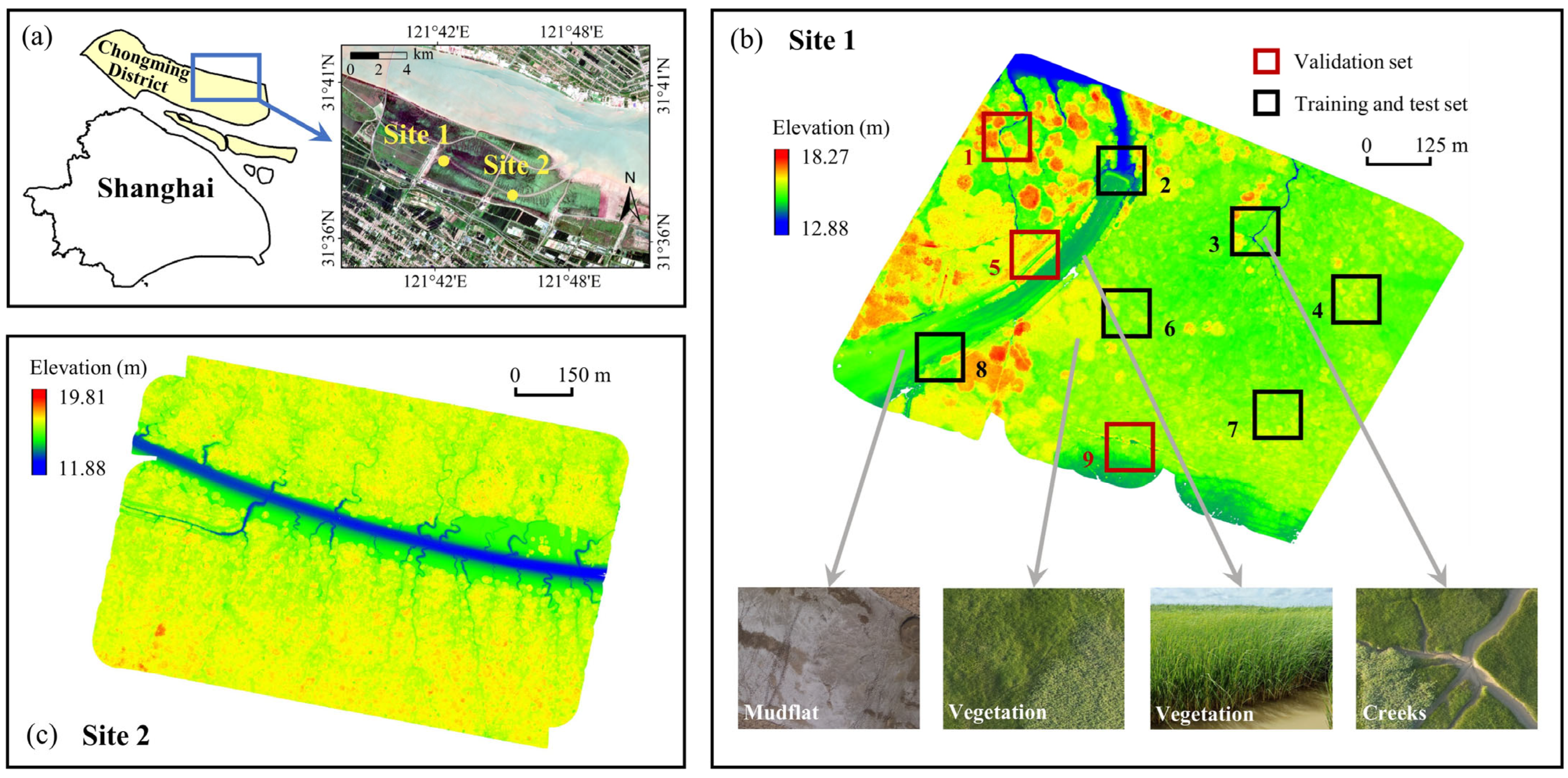
2.1. Materials

Two typical salt marshes (Figure 1) on Chongming Island at the mouth of the Yangtze River were selected as the study sites. Site 1 covers approximately 0.7 km² and is densely vegetated with two dominant vegetation species: Phragmites australis (PA) and Spartina alterniflora (SA). Site 2 covers approximately 1 km² and is densely vegetated with three dominant vegetation species: PA, SA, and Scirpus mariqueter (SM). The vegetation of the two sites ranges in height from 1 to 3 m and the distributions are spatially mixed. The overall terrain of the two sites is relatively flat. Geomorphologically, a long narrow mudflat runs north–south, dividing Site 1 into two vegetated sections, and several meandering creeks are distributed among the vegetated regions. In contrast, a wide tidal creek running from west to east lies in the middle of Site 2, which branches numerous narrow multilevel bifurcated creeks.

The point cloud data of the two study sites (Figure 1b,c) were acquired on 1 and 2 August 2023, using a DJI L1 LiDAR (SZ DJI Technology Co., Ltd., Shenzhen, China) mounted on a DJI Matrice 300 RTK drone (SZ DJI Technology Co., Ltd., Shenzhen, China). The DJI L1 is a 6-line LiDAR working at a wavelength of 905 nm. The maximum range is influenced by the reflectivity of the target surfaces, with a range of 450 m for surfaces with 80% reflectivity and 190 m for surfaces with 10% reflectivity. The DJI L1 supports two scanning modes: repetitive scanning and non-repetitive scanning. The repetitive scanning mode, similar to traditional linear LiDAR scanning mode, has a field of view (FOV) of 70.4° × 4.5° and can produce uniformly distributed and high precision point clouds. The non-repetitive scanning mode resembles a “flower petal” pattern, providing a nearly circular FOV (70.4° × 77.2°) that offers a stereo perspective of the scanned targets. Additionally, the DJI L1 can receive up to three laser echoes, which enhances its capability to penetrate vegetation and capture ground points. During the data collection of the two study sites, the drone was flown at a height of 100 m while moving uniformly at 7 m/s. The overlap rate of neighbor strips was 50%. The repetitive scanning mode was selected for data collection in this study. The collected data files were imported into DJI Terra 3.7.6 software for high-precision 3D reconstruction, resulting in LAS point cloud data in the WGS84 coordinate system. The main attributes of the LAS point cloud data include 3D coordinates (with z-coordinate/elevation being ellipsoidal height), intensity, scan angle, and GNSS time. Given that the ScanAngleRank field in the point cloud data collected by DJI L1 LiDAR represents the scan angle, only the distance needs to be derived (see Section 2.3.1). The obvious outliers in the point cloud data were manually removed using the CloudCompare 2.12.4 software, finally resulting in a total of 320,398,031 and 414,355,688 points for Site 1 and 2, with average densities of 458 and 414 points/m², respectively.

The training dataset should contain a diverse range of targets with different species, structures, and morphologies to enhance the generalization capability of the ANN model. In this study, six training sub-regions and three validation sub-regions of Site 1 (black and red boxes in Figure 1b), each covering an area of 100 × 100 m, were selected to build and evaluate the ANN model. The detailed information of the sub-regions is listed in

Table 1. Information of different sub-regions.

Dataset	Sub-Regions	Point Number	Vegetation	Topography Features
Training and test set	2	8,650,502	PA, SA, relatively dense	A part of bare muddy flat with undulating terrain
	3	7,725,041	PA, SA, highly dense	Several intertidal creeks
	4	3,965,034	SA, highly dense	Flat terrain and no intertidal creeks
	6	3,895,731	PA, SA, highly dense	Flat terrain and no intertidal creeks
	7	3,879,095	SA, highly dense	Flat terrain and no intertidal creeks
	8	5,301,961	PA, SA, relatively sparse	A part of bare muddy flat with flat terrain
Validation set	1	8,443,890	PA, SA, highly dense	Several intertidal creeks
	5	3,813,431	PA, relatively dense	A part of bare muddy flat with flat terrain
	9	4,523,592	PA, SA, relatively dense	Flat terrain and no intertidal creeks

. Randomly, a ratio of 7:3 of the points from the six training sub-regions were selected as the training and test sets, respectively. Site 2 was used to further verify the robustness and generalization of the ANN model. Several hyperparameters of the ANN model needed to be set beforehand, including hidden_layer_sizes, alpha, learning_rate_init, and max_iter. The grid searching method was employed to optimize these hyperparameters on the test set. The best values of the four hyperparameters in this study were (80, 80), 0.01, 0.001, and 100, respectively. Scikit-learn library in Python was adopted to implement the whole procedures of the ANN model. The reference data of the nine sub-regions were obtained through manual filtering using the CloudCompare 2.12.4 software, aided by the high-resolution orthophotos.

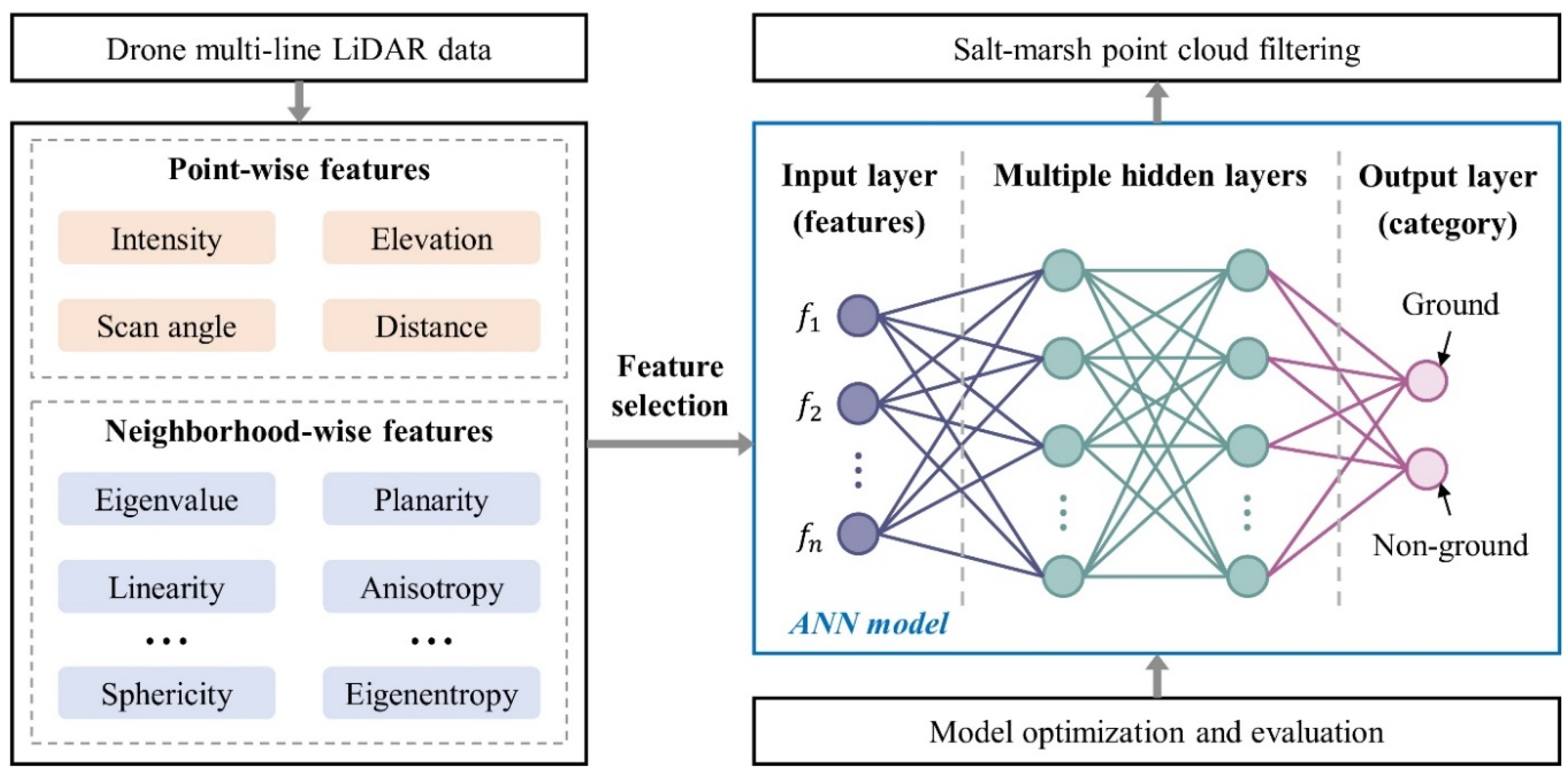
2.2. Overview of the Proposed Method

The general workflow of the proposed method is illustrated in Figure 2. A point $p_i=\left(x_i,y_i,z_i\right)$ together with its spherical neighborhood points within a radius $r$ in the acquired point cloud is defined as the set $N_m=\left\{p_i\left(x_i,y_i,z_i\right),i=\mathrm{1,2},\dots ,m\right\}$, where m is the number of neighborhood points. First, the eigenvalues of each point are deduced based on the set $N_m$ and a series of the corresponding local geometric features (e.g., normal vector, sphericity, planarity, linearity, normal change rate, and eigen entropy) are derived according to these eigenvalues. These features jointly constitute the neighborhood-wise features (

Table 2. Point-wise and neighborhood-wise features.

	Feature Name	Abbreviation	Formula
Point-wise features	Distance	d	[38]
	Scan angle	$\mathsf{\theta }$	[38]
	Intensity	I	/
	Elevation	Z	/
Neighborhood-wise features	Eigenvalue	${\mathsf{\lambda }}_1$$,{\mathsf{\lambda }}_2$$,{\mathsf{\lambda }}_3$	[49]
	Normal vector	(u, v, w)	Eigenvector corresponds to the minimum eigenvalue ${\mathsf{\lambda }}_3$
	Scattered feature	S	$\mathrm{S}=\sqrt{{\mathsf{\lambda }}_3}∕\sqrt{{\mathsf{\lambda }}_1}$
	Linear feature	L	$\mathrm{L}=\left(\sqrt{{\mathsf{\lambda }}_1}-\sqrt{{\mathsf{\lambda }}_2}\right)∕\sqrt{{\mathsf{\lambda }}_1}$
	Planar feature	P	$\mathrm{P}=\left(\sqrt{{\mathsf{\lambda }}_2}-\sqrt{{\mathsf{\lambda }}_3}\right)∕\sqrt{{\mathsf{\lambda }}_1}$
	Normal change rate	NCR	$\mathrm{N}\mathrm{C}\mathrm{R}={\mathsf{\lambda }}_3∕\left({\mathsf{\lambda }}_1+{\mathsf{\lambda }}_2+{\mathsf{\lambda }}_3\right)$
	Anisotropy	AN	$\mathrm{A}\mathrm{N}=\left({\mathsf{\lambda }}_1-{\mathsf{\lambda }}_3\right)∕{\mathsf{\lambda }}_1$
	Sphericity	SP	$\mathrm{S}\mathrm{P}={\mathsf{\lambda }}_3∕{\mathsf{\lambda }}_1$
	Linearity	LI	$\mathrm{L}\mathrm{I}=\left({\mathsf{\lambda }}_1-{\mathsf{\lambda }}_2\right)∕{\mathsf{\lambda }}_1$
	Planarity	PL	$\mathrm{P}\mathrm{L}=\left({\mathsf{\lambda }}_2-{\mathsf{\lambda }}_3\right)∕{\mathsf{\lambda }}_1$
	Sum of eigenvalues	ES	$\mathrm{E}\mathrm{S}={\mathsf{\lambda }}_1+{\mathsf{\lambda }}_2+{\mathsf{\lambda }}_3$
	Ominvariance	OMV	$\mathrm{O}\mathrm{M}\mathrm{V}=\sqrt[3]{{\mathsf{\lambda }}_1\times {\mathsf{\lambda }}_2\times {\mathsf{\lambda }}_3}$
	Eigen entropy	EN	$\mathrm{E}\mathrm{N}={\sum }_{\mathrm{i}=1}^3{\mathsf{\lambda }}_{\mathrm{i}}\times \log {\mathsf{\lambda }}_{\mathrm{i}}$

). Second, the instantaneous scan distance between the center of the LiDAR instrument and the scanned point and the scan angle between the incidence laser beam and the vertical direction is recovered, following the method in [38]. Third, the point-wise (individual scale) features (i.e., distance, scan angle, intensity, and elevation) and neighborhood-wise (neighborhood scale) features are combined as the input feature set. Selection is conducted on this set to remove redundant or irrelevant features. Fourth, the point cloud is divided into training, testing, and validation sets to train, optimize, and evaluate the ANN model, and the constructed model is finally adopted to filter the entire data. In this stage, the remained features are used as input features for the ANN model.

2.3. Features Derivation and Selection

Ground and non-ground/vegetation points differ not only in geometric and spectral features (e.g., elevation and intensity) at an individual scale [38] but also in spatial features at a neighborhood scale. For example, ground points locally exhibit a flat distribution, appearing planar spatially. By contrast, vegetation points are more scattered and can typically present linear or spherical characteristics. Therefore, subtle differences between ground and vegetation points can be fully exploited by integrating spatial and spectral features at individual and neighborhood scales.

2.3.1. Point-Wise Features

The original data of the drone multi-line LiDAR include the intensity value of each point that is tightly associated with the target reflectance. As shown in Figure 3, the original intensity values of non-ground/vegetation points are generally larger than that of ground points. This phenomenon is because salt marsh ground and vegetation have totally different materials and spectral reflectance. However, intensity is influenced by multiple factors, with distance and incidence angle being dominant [31], resulting in considerable overlap between the intensity values of ground and non-ground points (Figure 3). Therefore, original intensity data must be corrected before being used for filtering. Existing intensity correction models exhibit complexity and poor generalization ability, making it challenging to use intensity for point cloud filtering [17]. Our previous work has demonstrated that the complicated intensity correction procedure is dispensable if the original intensity along with its dominating influencing factors are input into a machine learning model [38]. Similarly, this study selects intensity ($I$), distance ($d$), and scan angle ($\theta$) as input individual-scale features. Due to the dynamic nature of the drone multi-line LiDAR scanning mode and the unavailability of the flight trajectory in the user-provided data, distance and scan angle cannot be directly obtained, and are recovered following the method proposed in [38]. Additionally, since vegetation points typically have higher elevations than ground points, the vertical coordinate ($Z$) is selected as an input feature. In summary, a total of four point-wise features are selected.

2.3.2. Neighborhood-Wise Features

Neighborhood-wise features are derived based on the 3D coordinates of the interesting point and its surrounding points within a certain spatial neighborhood. These features can demonstrate the spatial morphological characteristics of the point cloud from a local perspective [50]. For a given point $p_i$ with a neighborhood point cloud set $N_m$, the covariance matrix can be computed as follows:

$$C_{3\times 3}\left(N_m\right)={\displaystyle \frac{1}{m}}{\sum }_{i=1}^m\left(p_i-\overline{p}\right){\left(p_i-\overline{p}\right)}^T$$

(1)

where $\overline{p}=\left(1/m\right){\sum }_{i=1}^m\left(x_i,y_i,z_i\right)$ is the geometric center of the point cloud set $N_m$. The neighborhood of a point cloud is defined as a spherical space with a radius of $r$, and $r$ was set to 0.5 m to ensure accurate extraction of local geometric features in this study. After obtaining the covariance matrix $C_{3\times 3}\left(N_m\right)$, singular value decomposition (SVD) or similar methods can be used to calculate the three eigenvalues which are sorted in descending order as ${\mathsf{\lambda }}_1\ge {\mathsf{\lambda }}_2{\ge \mathsf{\lambda }}_3$. Afterwards, a series of eigenvalue-based geometric features (Table 2) can be derived [51,52]. Together with the 3 eigenvalues, a total of 17 neighborhood-wise features are preliminary selected.

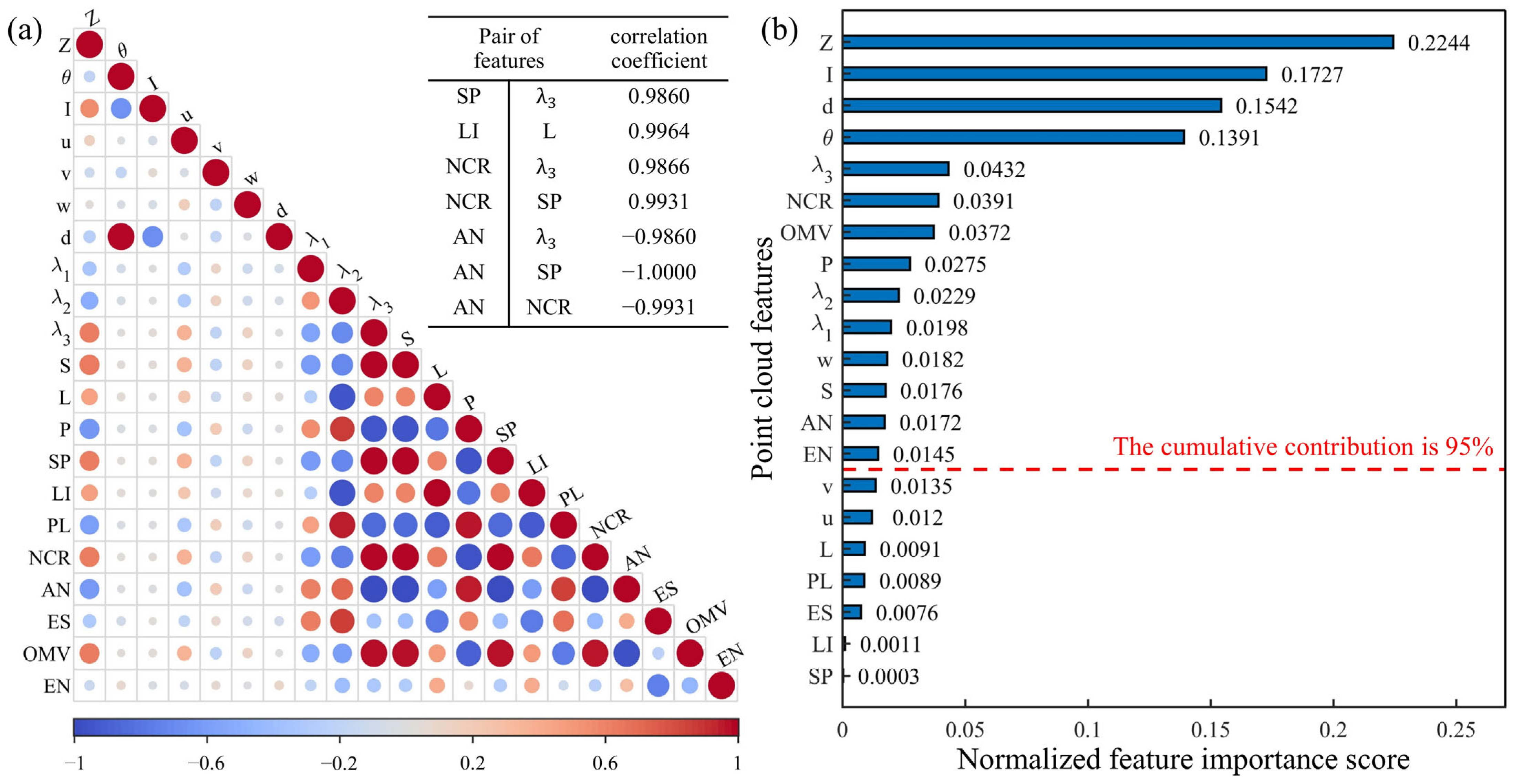
2.3.3. Feature Selection

As introduced in Section 2.3.1 and Section 2.3.2, a total of 21 features (i.e., 4 point-wise and 17 neighborhood-wise features) constitute the feature set. Appropriate features can enhance the filtering accuracy of ANN. By contrast, superfluous features can downgrade the computational efficiency and performance of ANN, particularly when several redundant or irrelevant features are contained [53]. Therefore, prior feature selection is typically essential to remove redundant and irrelevant features. In this study, a feature selection tool developed by [54] is employed to perform feature selection on the 21 features. This tool selects features based on five criteria. (1) Features with large missing data are considered invalid and removed. (2) Features with only a single value are discarded. (3) Highly correlated features are identified as redundant, and one feature from each correlated pair is eliminated. (4) The dataset is trained multiple times using LightGBM to compute feature importance scores, and features with a score of zero are excluded. (5) Based on the importance scores from (4), features contributing cumulatively beyond a specified threshold (the commonly used threshold is 95% and was adopted in this study) are removed.

2.4. ANN-Based Point Cloud Filtering

ANN simulates the information processing mechanisms of biological neurons, enabling efficient learning from vast amounts of data and accurately establishing the functional mapping between inputs and outputs. The basic building block of ANN is the neuron. ANN consists of an input layer and an output layer, together with one or more hidden layers (Figure 2). Each layer comprises multiple neurons, and the hidden layers can consist of several hierarchical levels. Neurons in different layers are fully connected, forming a comprehensive network structure (Figure 2). This network structure allows ANN to approximate various nonlinear functions effectively. Assume the input signal to an ANN neuron is $\mathrm{X}$, the weight is $\mathrm{W}$, the bias is $\mathrm{b}$, and the activation function is $\mathsf{\phi }$. The output signal $\mathrm{P}$ of the neuron is given by

$$\mathrm{P}=\mathsf{\phi }\left(\mathrm{W}{\mathrm{X}}^{\mathrm{T}}+\mathrm{b}\right)$$

(2)

Each neuron in the hidden layers of the ANN processes samples according to Equation (2). When a sample with a known true value is input into the ANN model, it undergoes forward propagation through the network, resulting in a predicted value. The error between the true and predicted values is then calculated and backpropagated through the hidden neurons to update the weight parameters. This constitutes one learning iteration for a single sample. By inputting multiple training samples and iterating through numerous learning cycles until the acceptable error threshold is reached, the training process is completed. ANN is adaptive and capable of automatically adjusting weights and biases to accommodate different inputs and outputs.

2.5. Accuracy Evaluation

The dense vegetation coverage in salt marshes results in a relatively low proportion of ground points, though drone multi-line LiDAR shows prominent penetrability. This leads to a high imbalance in terms of the amounts of ground and non-ground points. In such scenarios, commonly used classification evaluation metrics, e.g., overall accuracy, are unsuitable. Therefore, the area under the curve (AUC) [55] of the receiver operating characteristics (ROC) and the geometric mean (G—mean, Equation (3)) [56] are adopted as quantitative evaluation metrics for the point cloud filtering results, which are more appropriate for assessing imbalanced sample classification performance. Let TP and TN be the number of ground and non-ground points correctly classified, respectively. By contrast, FB and FP are defined as the number of ground and non-ground points incorrectly classified, respectively. By varying the model classification threshold, multiple sets of false positive rates (FPR = FP/(TN + FP)) and true positive rates (TPR = TP/(TP + FN)) can be obtained. The ROC curve is plotted with FPR on the x-axis and TPR on the y-axis. The area under the ROC curve is denoted as AUC. The range of AUC and G—mean is between 0 and 1, with higher values denoting better filtering performance.

$$\mathrm{G}-\mathrm{m}\mathrm{e}\mathrm{a}\mathrm{n}=\sqrt{{\displaystyle \frac{\mathrm{T}\mathrm{N}}{\mathrm{T}\mathrm{N}+\mathrm{F}\mathrm{P}}}\times {\displaystyle \frac{\mathrm{T}\mathrm{P}}{\mathrm{T}\mathrm{P}+\mathrm{F}\mathrm{N}}}}$$

(3)

3. Results

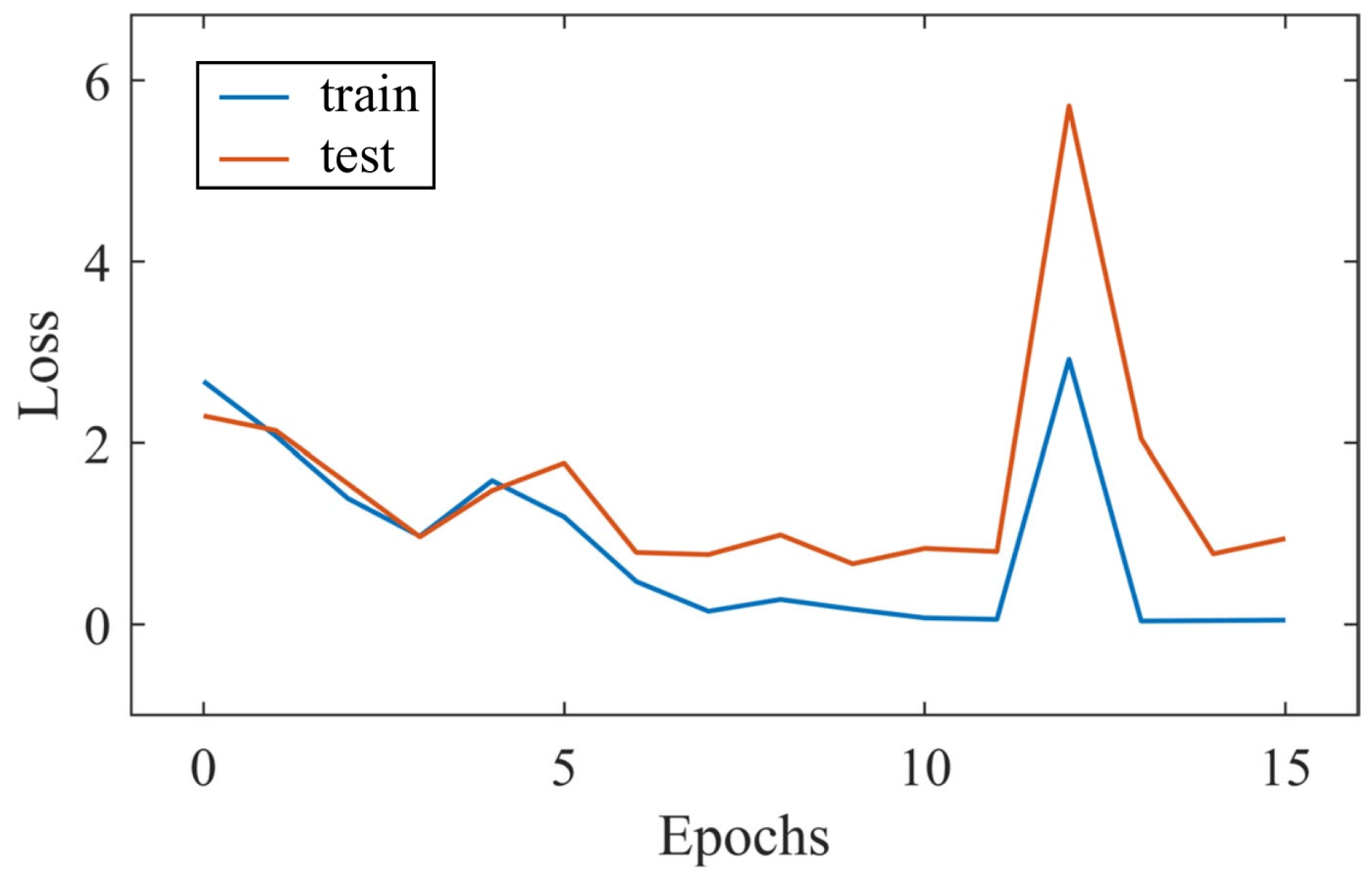
3.1. Results of Training and Test Sets

According to the five criteria of the feature selection tool developed by [54], the 21 preliminary features were selected, as follows. (1) No features with significant data missing were identified. (2) No features containing only a single value existed. (3) The Pearson correlation coefficient matrix (Figure 4a) revealed that seven pairs of features (i.e., SP and ${\mathsf{\lambda }}_3$, LI and L, NCR and ${\mathsf{\lambda }}_3$, NCR and SP, AN and ${\mathsf{\lambda }}_3$, AN and SP, and AN and NCR) have strong correlations. Consequently, one feature from each correlated pair should be removed. In this study, SP, LI, NCR, and AN were removed. (4) Multiple trainings with LightGBM provided a ranking of feature importance (Figure 4b). No features had an importance score of zero. (5) The features, including v, u, L, PL, ES, LI, and SP, were considered low-contribution features (Figure 4b) because the cumulative contribution (sum of importance scores) exceeded 95% when features were ranked by the importance score. Based on the comprehensive assessment of these five perspectives, the features SP, LI, NCR, AN, v, u, L, PL, and ES were excluded. The remaining 12 features, i.e., point-wise (4) distance (d), scan angle ($\mathsf{\theta }$), intensity (I), and elevation (Z), and neighborhood-wise (8) eigenvalue (${\mathsf{\lambda }}_1$, ${\mathsf{\lambda }}_2$, ${\mathsf{\lambda }}_3$), vertical coordinates of normal vector (w), scattered feature (S), planar feature (P), ominvariance (OMV), and eigen entropy (EN), were finally adopted as the input features of the ANN model.

The filtering results for the training and test sets are shown in Figure 5. Evidently, the proposed method achieved satisfactory filtering performance across the six training sub-regions. In particular, the majority of the mudflat was accurately recognized as ground points in sub-regions 2 and 8, with only a few points on the protuberance parts being misclassified as vegetation points (blue elliptical areas in Figure 5). The curved creeks in sub-region 3 were effectively identified as ground points. Despite the highly dense vegetation and sparse ground point coverage in sub-regions 4, 6, and 7, the ANN model successfully distinguished between vegetation and ground points. The values of the metrics (AUC and G-mean) were 0.9703 and 0.9702 for the training set, whereas those for the test sets were 0.9702 and 0.9701. In conclusion, the ANN model is proficient in self-learning the spatial and spectral characteristics of vegetation and ground points by the selected features at individual and neighborhood scales, achieving high-precision and intelligent point cloud filtering.

3.2. Results of Validation Set

The filtering results of the validation set by the constructed ANN model are shown in Figure 6. Apparently, the vegetation and ground points in the three validation sub-regions were accurately discriminated. The creeks in sub-region 1 and the mudflats in sub-regions 5 and 9 were effectively identified as ground points. The AUC and G-mean for the three sub-regions 1, 5, and 9 were 0.9895 and 0.9895, 0.9241 and 0.9214, and 0.9214 and 0.9208, respectively. The results indicate that the trained ANN model demonstrates satisfactory transferability and generalization ability and can achieve high filtering accuracy when applied to unknown data. Sub-region 1 achieved the highest filtering accuracy among the three validation sub-regions, mainly due to the distinct boundary between the creeks and the adjacent vegetation. In contrast, sub-regions 5 and 9 have mixed distributions of mudflats and vegetation, confusing their morphological characteristics and presenting challenges for the ANN model during filtering. Additionally, even with the aid of high-resolution imagery, manual filtering in these sub-regions is difficult, resulting in slight deviations in the quantitative evaluation results for sub-regions 5 and 9.

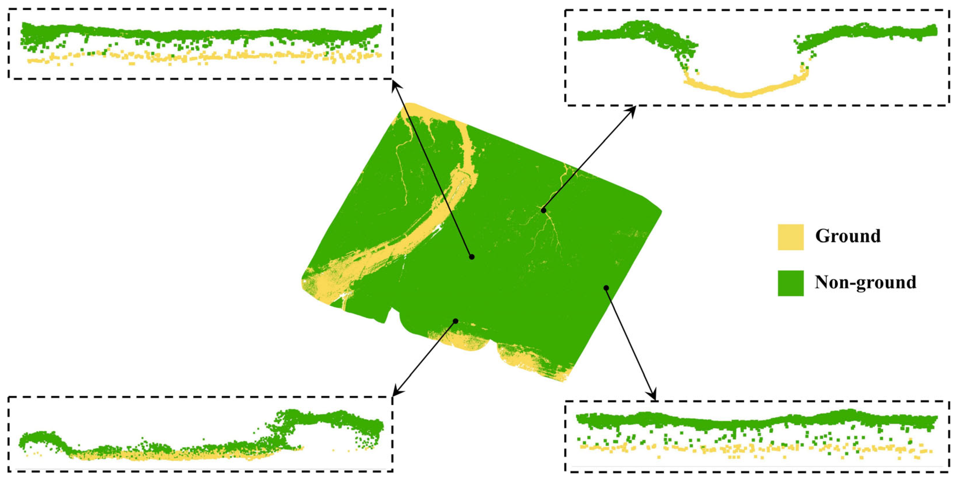
3.3. Filtering Results of Site 1

The filtering results of Site 1 by the proposed method are shown in Figure 7a, Figure 7h, and Figure A1. Regardless of the density and distribution of the vegetation, the ground points could be successfully identified. Specifically, the north–south-oriented mudflat and the creeks distributed among the vegetation were effectively recognized as ground points. Statistically, the number of ground points in the study site is 37,234,012, accounting for only a very small portion of the total point cloud. Notably, the ground points directly beneath each drone flight strip were denser, leading to an evident “strip effect” in the ground points (Figure 7h). This density heterogeneity is probably because the incidence angles of these points beneath the drone trajectory were nearly 0°. As such, the laser beams could more easily penetrate perpendicularly to the ground.

4. Discussion

4.1. Comparison of Different Methods

To further demonstrate the superiority of the ANN model for filtering drone multi-line LiDAR point clouds in salt marshes, we compared its performance against three machine learning algorithms (RF, XGBoost, and LightGBM), three commonly used point cloud filtering methods (SF, PMF, and CSF), and a deep learning model (RandLA-Net), as shown by Figure 7 and Figure 8. RF, XGBoost, and LightGBM were trained using the same training and test sets and the same features as the ANN and optimized through the grid search method for the best hyperparameters to ensure a fair comparison. Similarly, SF, PMF, and CSF were iteratively adjusted to their optimal parameters to obtain the best filtering results for comparison. Due to the differences in the training process between deep learning models and the ANN model, the training and test sets used for the ANN model in this study cannot be directly applied to the RandLA-Net model. Therefore, we re-partitioned the datasets to suit the training of the RandLA-Net model. Sub-regions 2, 3, 4, 6, 7, and 8 were still selected as the training dataset. For each sub-region, the left 30% was used as the test set, while the right 70% was used as the training set. The model training was completed when the loss on the test set no longer decreased.

RF, XGBoost, and LightGBM were implemented using the Scikit-learn, XGBoost, and LightGBM libraries in Python, respectively. The best parameters of the three machine learning models are listed in

Table 3. Best parameters of different machine learning methods.

Methods	Learning Rate	Max_Depth	n_Estimators	Min_Samples_Leaf/Min_Child_Weight	Gamma
RF	NA	9	50	1000	NA
XGBoost	0.1	10	500	1	0.1
LightGBM	0.1	10	600	1	NA

. SF was implemented using MATLAB code. The primary parameter for this method is the slope, with 5° identified as the optimal value. PMF was implemented using the point cloud library (PCL) in Python. The primary parameters include MaxWindowSize, Slope, InitialDistance, and MaxDistance. The optimal values for these parameters were 5, 0.1, 0.2, and 1, respectively. CSF was implemented using the CSF library in Python. The primary parameters include rigidness, cloth_resolution, class_threshold, and iterations, whose optimal values were 3, 0.9, 0.3, and 400, respectively. RandLA-Net was implemented using ArcGIS Pro 3.1.6 software. The RandLA-Net model was trained in 25 epochs at a batch size of 8 blocks with a block size of 4 m. The loss curves during the training of the RandLA-Net model are shown in Figure A3 (Appendix B).

The comparison results indicated that SF, PMF, CSF, and RandLA-Net performed remarkably worse than the machine learning methods, displaying noticeable misclassifications between ground and vegetation points. Specifically, evident misclassification occurred around the shores of the creeks for the SF method where substantial ground points were identified as vegetation (Figure 7m). Additionally, a large number of vegetation points in the vegetation-rich areas were recognized as ground (Figure 8m–o). Contrary to the “strip effect” in the ground points of the ANN method, this phenomenon occurred in the vegetation points of the SF method (Figure 7e). As for the PMF method, a majority of the mudflat points were identified as vegetation (Figure 7f). Moreover, the creeks were visually undetectable from the ground points and a considerable proportion of vegetation points were misclassified in the filtering process (Figure 7n and Figure 8p–r). Very similar filtering performance with respect to the shores of creeks was acquired by the CSF method. The difference was that more vegetation points were incorrectly distinguished as the ground in the dense vegetation regions (Figure 7o and Figure 8s–u). As for the RandLA-Net model, the filtering performance was similar to that of the PMF, with a large number of vegetation points being misclassified as ground points (Figure 7p and Figure 8v–x). The difference was that the mudflat points were correctly classified as ground points by PMF (Figure 7h). Expectedly, RF, XGBoost, and LightGBM showed very similar performance to that of the ANN, achieving relatively satisfactory filtering results. This is because SF, PMF, CSF, and RandLA-Net rely solely on the spatial features of the point cloud, making it challenging to accurately separate the dense and morphologically diverse salt marsh vegetation from the ground. Machine learning methods, on the other hand, utilize individual and neighborhood spatial and spectral features to automatically learn the distinctions between vegetation and ground points from multiple dimensions, leading to superior filtering results.

Quantitative comparisons were conducted on the validation set (

Table 4. Metrics of different filtering methods using different features on the validation set.

	Sub-Region 1		Sub-Region 5		Sub-Region 9
	AUC	G-Mean	AUC	G-Mean	AUC	G-Mean
ANN	0.9895	0.9895	0.9241	0.9219	0.9214	0.9208
RF	0.9915	0.9915	0.9178	0.9148	0.9205	0.9198
XGBoost	0.9960	0.9960	0.9115	0.9076	0.8838	0.8804
LightGBM	0.9961	0.9961	0.9118	0.9079	0.8820	0.8783
SF	0.8011	0.8009	0.9055	0.9051	0.7657	0.7652
PMF	0.8601	0.8522	0.9296	0.9281	0.7921	0.7886
CSF	0.8515	0.8408	0.9083	0.9037	0.7029	0.6384
RandLA-Net	0.8556	0.8436	0.8738	0.8683	0.9029	0.8993
Point-wise features	0.9815	0.9814	0.8862	0.8824	0.9136	0.9136
Neighborhood-wise features	0.5977	0.4518	0.6909	0.6197	0.6435	0.5675

). While LightGBM and PMF achieved the highest AUC and G-mean in sub-regions 1 and 5, respectively, their performance only slightly surpassed that of the ANN and was clearly inferior to the ANN in sub-region 9. Overall, the ANN demonstrated consistently good filtering results across all sub-regions, showcasing greater robustness and stability. The ANN utilizes a multi-layer network structure and nonlinear activation functions (e.g., ReLU and Sigmoid) to effectively fit complex nonlinear mapping relationships. This capacity enables ANN to capture and express subtle differences between ground and non-ground points in salt marshes more accurately than decision tree-based machine learning methods (e.g., RF, XGBoost, and LightGBM), which have relatively limited nonlinear fitting capabilities. Moreover, the hidden layers in ANN can combine input features to create higher-dimensional features, allowing for the learning of more advantageous feature combinations during filtering. In contrast, RF, XGBoost, and LightGBM primarily depend on manually inputted features, resulting in less feature depth and complexity compared to ANN. Although RandLA-Net also extracts features at individual and neighborhood scales, it may not sufficiently capture the differences between the irregularly shaped vegetation points and sparse ground points, leading to lower filtering accuracy compared to ANN. In sub-region 5, there is no significant difference in the performance of the four machine learning methods and the three traditional filtering methods, with PMF exhibiting marginally superior filtering accuracy. This is because sub-region 5 contains a substantial area of mudflats clearly separated from vegetation and the relatively low imbalance in the number of vegetation and ground points (the radios of vegetation-to-ground points in sub-regions 1, 5, and 9 were 15.29, 2.93, and 10.79, respectively). Consequently, these methods can achieve similar filtering results in vegetation- and mudflat-dominated areas. The utilization of morphological erosion and dilation operations by PMF enhances its ability to detect abrupt changes, leading to better filtering results at vegetation and mudflat boundaries, thereby achieving the highest filtering accuracy in sub-region 5.

4.2. Comparison of Different Features

To demonstrate the advantages of filtering by integrating features at different scales, we conducted ANN model training, testing, and validation using either point-wise features (Z, I, d, and $\mathsf{\theta }$) or neighborhood-wise features (${\mathsf{\lambda }}_3$, OMV, P, ${\mathsf{\lambda }}_2$, ${\mathsf{\lambda }}_1$, w, S, and EN). The training, test, and validation sets used were consistent with those in Section 3.2 and Section 3.3, with hyperparameters optimized via the grid searching method. The filtering results are demonstrated in Figure 9 and Figure 10 and Table 4. As expected, using only point-wise features leads to slightly poorer performance, with some vegetation points near the creeks being misclassified as ground points (Figure 9a and Figure 10a). This misclassification occurs mainly because these vegetation points are adjacent to the ground, making their elevation and intensity similar to those of the ground. Accordingly, using only neighborhood-wise features resulted in significant misclassification, with the AUC and G-mean for the three validation sub-regions being 0.5977 and 0.4518, 0.6909 and 0.6197, and 0.6435 and 0.5675, respectively. According to the feature importance score in Section 3.1 (Figure 4b), point-wise features generally have higher importance than neighborhood features, indicating that point-wise features dominate the filtering results. Combining point-wise and neighborhood-wise features can compensate for the limitations of using single-scale features, achieving optimal point cloud filtering performance.

4.3. Generalization Performance of the Proposed Method

To further verify the robustness and generalization of the proposed method, we used Site 2 to evaluate the performance of the ANN model trained by Site 1, as shown in Figure 11 and Figure A2. Obviously, dense vegetation was effectively distinguished, and the wide tidal creek in the middle of Site 2 was accurately classified as ground points. Additionally, the spatial distribution and orientation of the narrow tidal creeks within the densely vegetated areas were clearly visible from the filtered ground points. Similar to Site 1, the ground points in Site 2 also exhibited an evident “strip effect” (Figure 11b). Three representative sub-regions in Site 2 (sub-regions A, B, and C, located in the black rectangular areas in Figure 11a) were selected to quantitatively assess the filtering accuracy (Figure 12). The vegetation in sub-regions A and C are highly dense, while that in sub-region B is less dense. Sub-region A includes two narrow tidal creeks. Sub-region B includes a wide tidal creek and a part of a bare mudflat. Sub-region C is completely covered by vegetation with no tidal creeks. The AUC and G-mean for the three sub-regions were 0.9689 and 0.9688, 0.9742 and 0.9740, and 0.9112 and 0.9069, respectively. The results indicate that the trained ANN model can still achieve high filtering accuracy when applied to other salt marshes. In sub-regions A and B, the tidal creeks and mudflats were accurately classified as ground points (Figure 12d,e), and the dense vegetation in sub-region C was also correctly identified. However, the filtering accuracy in sub-region C was slightly lower than that in sub-regions A and B. This was due to the extremely dense vegetation coverage, which led to sparse ground points and increased the difficulty of filtering. Overall, the proposed method demonstrates strong applicability and robustness across different salt marshes.

In practical applications, directly applying the model trained in this study to other salt marsh point clouds acquired by different drone LiDAR instruments with diverse vegetation species and varying environmental conditions may lead to suboptimal results. A new ANN model should be constructed following the proposed method in these circumstances. The major procedures include feature derivation and selection, model training and construction, and model validation and application (Figure 2). The proposed method does not require complex parameterization and prior knowledge of the specific scene or dataset. Only the fundamental derived features are needed. Additionally, the proposed method provides a novel strategy for massive drone LiDAR point cloud filtering and can be applied to regions beyond coastal salt marshes (e.g., forest, urban, and mountainous).

4.4. Analysis of the Impact of Feature Selection

To analyze the impact of feature selection on the filtering results, we trained, tested, and validated the ANN model using all 21 features (Table 2) without feature selection. The training set, test set, validation set, and hyperparameter optimization method were consistent with those employed in the experiments with feature selection (Section 3). The filtering results on the validation set of Site 1 are shown in Figure 13. The AUC and G-mean for the three validation sub-regions were 0.9894 and 0.9894, 0.9229 and 0.9205, and 0.9168 and 0.9160, respectively. The experiments with or without feature selection were both conducted on a desktop (32 GB RAM and Inter Core i7-11700K CPU at 3.6 GHz). The training time for the ANN model without feature selection was 5.25 h, while that was 3.27 h for the ANN model with feature selection. The results demonstrate that feature selection does not considerably improve the filtering accuracy of the ANN model. However, feature selection can effectively reduce the training time, playing a key role in enhancing computational efficiency.

5. Conclusions

This study proposes an ANN-based filtering method for salt marsh point clouds of drone multi-line LiDAR, which deeply combines spectral and spatial features at individual and neighborhood scales and provides an alternative strategy for salt marsh point cloud interpretation. The proposed method can autonomously and efficiently learn the distinctions between ground and non-ground points. The trained ANN model achieved an averaged AUC and G-mean of 0.9450 and 0.9441, outperforming RF, XGBoost, LightGBM, SF, PMF, CSF, and RandLA-Net and the filtering solutions by only point-wise or neighborhood-wise features alone. However, the ecological and geographical conditions of salt marshes are highly complex, with varying vegetation types, landforms, and dynamic processes across different regions, leading to great differences in the spatial and spectral characteristics of point cloud data. Future research could further analyze the applicability of the proposed filtering method to different salt marsh regions. Moreover, this method could be broadened to point cloud filtering in other coastal and land landscapes, e.g., mangroves and arbor forests. This study only selected a single neighborhood radius to calculate neighborhood-wise features. Deriving multi-scale neighborhood features and constructing more spectral–spatial features can further improve the accuracy, robustness, and intelligence of the proposed method in future work.

References

1. Adams, J.B. Salt marsh at the tip of Africa: Patterns, processes and changes in response to climate change. Estuar. Coast. Shelf Sci. 2020, 237, 106650. [Google Scholar] [CrossRef]
2. Wang, F.M.; Sanders, C.J.; Santos, I.R.; Tang, J.W.; Schuerch, M.; Kirwan, M.L.; Kopp, R.E.; Zhu, K.; Li, X.Z.; Yuan, J.C.; et al. Global blue carbon accumulation in tidal wetlands increases with climate change. Natl. Sci. Rev. 2021, 8, nwaa296. [Google Scholar] [CrossRef] [PubMed]
3. Campbell, A.D.; Fatoyinbo, L.; Goldberg, L.; Lagomasino, D. Global hotspots of salt marsh change and carbon emissions. Nature 2022, 612, 701–706. [Google Scholar] [CrossRef] [PubMed]
4. Jin, C.; Gong, Z.; Shi, L.; Zhao, K.; Tinoco, R.O.; San Juan, J.E.; Geng, L.; Coco, G. Medium-term observations of salt marsh morphodynamics. Front. Mar. Sci. 2022, 9, 988240. [Google Scholar] [CrossRef]
5. Tan, K.; Chen, J.; Zhang, W.G.; Liu, K.B.; Tao, P.J.; Cheng, X.J. Estimation of soil surface water contents for intertidal mudflats using a near-infrared long-range terrestrial laser scanner. ISPRS-J. Photogramm. Remote Sens. 2020, 159, 129–139. [Google Scholar] [CrossRef]
6. Tang, Y.N.; Ma, J.; Xu, J.X.; Wu, W.B.; Wang, Y.C.; Guo, H.Q. Assessing the impacts of tidal creeks on the spatial patterns of coastal salt marsh vegetation and its aboveground biomass. Remote Sens. 2022, 14, 1839. [Google Scholar] [CrossRef]
7. Molino, G.D.; Defne, Z.; Aretxabaleta, A.L.; Ganju, N.K.; Carr, J.A. Quantifying slopes as a driver of forest to marsh conversion using geospatial techniques: Application to Chesapeake Bay Coastal-Plain, United States. Front. Environ. Sci. 2021, 9, 616319. [Google Scholar] [CrossRef]
8. Sandi, S.G.; Rodríguez, J.F.; Saintilan, N.; Riccardi, G.; Saco, P.M. Rising tides, rising gates: The complex ecogeomorphic response of coastal wetlands to sea-level rise and human interventions. Adv. Water Resour. 2018, 114, 135–148. [Google Scholar] [CrossRef]
9. Yi, W.B.; Wang, N.; Yu, H.Y.; Jiang, Y.H.; Zhang, D.; Li, X.Y.; Lv, L.; Xie, Z.L. An enhanced monitoring method for spatio-temporal dynamics of salt marsh vegetation using google earth engine. Estuar. Coast. Shelf Sci. 2024, 298, 108658. [Google Scholar] [CrossRef]
10. Gao, W.L.; Shen, F.; Tan, K.; Zhang, W.G.; Liu, Q.X.; Lam, N.S.N.; Ge, J.Z. Monitoring terrain elevation of intertidal wetlands by utilising the spatial-temporal fusion of multi-source satellite data: A case study in the Yangtze (Changjiang) Estuary. Geomorphology 2021, 383, 107683. [Google Scholar] [CrossRef]
11. Yang, B.X.; Ali, F.; Zhou, B.; Li, S.L.; Yu, Y.; Yang, T.T.; Liu, X.F.; Liang, Z.Y.; Zhang, K.C. A novel approach of efficient 3D reconstruction for real scene using unmanned aerial vehicle oblique photogrammetry with five cameras. Comput. Electr. Eng. 2022, 99, 107804. [Google Scholar] [CrossRef]
12. Taddia, Y.; Pellegrinelli, A.; Corbau, C.; Franchi, G.; Staver, L.W.; Stevenson, J.C.; Nardin, W. High-resolution monitoring of tidal systems using UAV: A case study on Poplar Island, MD (USA). Remote Sens. 2021, 13, 1364. [Google Scholar] [CrossRef]
13. An, S.K.; Yuan, L.; Xu, Y.; Wang, X.; Zhou, D.W. Ground subsidence monitoring in based on UAV-LiDAR technology: A case study of a mine in the Ordos, China. Geomech. Geophys. Geo-Energy Geo-Resour. 2024, 10, 57. [Google Scholar] [CrossRef]
14. Hodges, E.; Campbell, J.D.; Melebari, A.; Bringer, A.; Johnson, J.T.; Moghaddam, M. Using Lidar digital elevation models for reflectometry land applications. IEEE Trans. Geosci. Remote Sensing 2023, 61, 5800509. [Google Scholar] [CrossRef]
15. Jancewicz, K.; Porebna, W. Point cloud does matter. Selected issues of using airborne LiDAR elevation data in geomorphometric studies of rugged sandstone terrain under forest—Case study from Central Europe. Geomorphology 2022, 412, 108316. [Google Scholar] [CrossRef]
16. Medeiros, S.C.; Bobinsky, J.S.; Abdelwahab, K. Locality of topographic ground truth data for salt marsh LiDAR DEM elevation bias mitigation. IEEE J. Sel. Top. Appl. Earth Observ. Remote Sens. 2022, 15, 5766–5775. [Google Scholar] [CrossRef]
17. Tao, P.J.; Tan, K.; Ke, T.; Liu, S.; Zhang, W.G.; Yang, J.R.; Zhu, X.J. Recognition of ecological vegetation fairy circles in intertidal salt marshes from UAV LiDAR point clouds. Int. J. Appl. Earth Obs. Geoinf. 2022, 114, 103029. [Google Scholar] [CrossRef]
18. Cai, S.S.; Liang, X.L.; Yu, S.S. A progressive plane detection filtering method for airborne LiDAR data in forested landscapes. Forests 2023, 14, 498. [Google Scholar] [CrossRef]
19. Vosselman, G. Slope based filtering of laser altimetry data. Int. Arch. Photogramm. Remote Sens. 2000, 33, 935–942. [Google Scholar]
20. Zhang, W.M.; Qi, J.B.; Wan, P.; Wang, H.T.; Xie, D.H.; Wang, X.Y.; Yan, G.J. An easy-to-use airborne LiDAR data filtering method based on cloth simulation. Remote Sens. 2016, 8, 501. [Google Scholar] [CrossRef]
21. Zhang, K.Q.; Chen, S.C.; Whitman, D.; Shyu, M.L.; Yan, J.H.; Zhang, C.C. A progressive morphological filter for removing nonground measurements from airborne LIDAR data. IEEE Trans. Geosci. Remote Sens. 2003, 41, 872–882. [Google Scholar] [CrossRef]
22. Cai, S.S.; Yu, S.S.; Hui, Z.Y.; Tang, Z.Z. ICSF: An improved cloth simulation filtering algorithm for airborne LiDAR data based on morphological operations. Forests 2023, 14, 1520. [Google Scholar] [CrossRef]
23. Li, H.F.; Ye, C.M.; Guo, Z.X.; Wei, R.L.; Wang, L.X.; Li, J. A fast progressive TIN densification filtering algorithm for airborne LiDAR data using adjacent surface information. IEEE J. Sel. Top. Appl. Earth Observ. Remote Sens. 2021, 14, 12492–12503. [Google Scholar] [CrossRef]
24. Brodu, N.; Lague, D. 3D terrestrial lidar data classification of complex natural scenes using a multi-scale dimensionality criterion: Applications in geomorphology. ISPRS-J. Photogramm. Remote Sens. 2012, 68, 121–134. [Google Scholar] [CrossRef]
25. Stroner, M.; Urban, R.; Lidmila, M.; Kolar, V.; Kremen, T. Vegetation filtering of a steep rugged terrain: The performance of standard algorithms and a newly proposed workflow on an example of a railway ledge. Remote Sens. 2021, 13, 3050. [Google Scholar] [CrossRef]
26. Nesbit, P.R.; Hubbard, S.M.; Hugenholtz, C.H. Direct georeferencing UAV-SfM in high-relief topography: Accuracy assessment and alternative ground control strategies along steep inaccessible rock slopes. Remote Sens. 2022, 14, 490. [Google Scholar] [CrossRef]
27. Stroner, M.; Urban, R.; Línková, L. Multidirectional shift rasterization (MDSR) algorithm for effective identification of ground in dense point clouds. Remote Sens. 2022, 14, 4916. [Google Scholar] [CrossRef]
28. Anders, N.; Valente, J.; Masselink, R.; Keesstra, S. Comparing filtering techniques for removing vegetation from UAV-based photogrammetric point clouds. Drones 2019, 3, 61. [Google Scholar] [CrossRef]
29. Qin, N.N.; Tan, W.K.; Guan, H.Y.; Wang, L.Y.; Ma, L.F.; Tao, P.J.; Fatholahi, S.; Hu, X.Y.; Li, J.A.T. Towards intelligent ground filtering of large-scale topographic point clouds: A comprehensive survey. Int. J. Appl. Earth Obs. Geoinf. 2023, 125, 103566. [Google Scholar] [CrossRef]
30. Bai, J.; Niu, Z.; Gao, S.; Bi, K.Y.; Wang, J.; Huang, Y.R.; Sun, G. An exploration, analysis, and correction of the distance effect on terrestrial hyperspectral LiDAR data. ISPRS-J. Photogramm. Remote Sens. 2023, 198, 60–83. [Google Scholar] [CrossRef]
31. Tan, K.; Cheng, X.J. Correction of incidence angle and distance effects on TLS intensity data based on reference targets. Remote Sens. 2016, 8, 251. [Google Scholar] [CrossRef]
32. Breiman, L. Random forests. Mach. Learing 2001, 45, 5–32. [Google Scholar] [CrossRef]
33. Chen, T.Q.; Guestrin, C.; Assoc Comp, M. XGBoost: A scalable tree boosting system. In Proceedings of the 22nd ACM SIGKDD International Conference on Knowledge Discovery and Data Mining (KDD), San Francisco, CA, USA, 13–17 August 2016. [Google Scholar]
34. Ke, G.L.; Meng, Q.; Finley, T.; Wang, T.F.; Chen, W.; Ma, W.D.; Ye, Q.W.; Liu, T.Y. LightGBM: A highly efficient gradient boosting decision tree. In Proceedings of the 31st Annual Conference on Neural Information Processing Systems (NIPS), Long Beach, CA, USA, 4–9 December 2017. [Google Scholar]
35. Lettvin, J.Y.; Maturana, H.R.; McCulloch, W.S.; Pitts, W.H. What the frog’s eye tells the frog’s brain. Proc. IRE 1959, 47, 1940–1951. [Google Scholar] [CrossRef]
36. Duran, Z.; Ozcan, K.; Atik, M.E. Classification of photogrammetric and airborne LiDAR point clouds using machine learning algorithms. Drones 2021, 5, 104. [Google Scholar] [CrossRef]
37. Liao, L.F.; Tang, S.J.; Liao, J.H.; Li, X.M.; Wang, W.X.; Li, Y.X.; Guo, R.Z. A supervoxel-based random forest method for robust and effective airborne LiDAR point cloud classification. Remote Sens. 2022, 14, 1516. [Google Scholar] [CrossRef]
38. Wu, X.X.; Tan, K.; Liu, S.; Wang, F.; Tao, P.J.; Wang, Y.J.; Cheng, X.L. Drone multiline light detection and ranging data filtering in coastal salt marshes using extreme gradient boosting model. Drones 2024, 8, 13. [Google Scholar] [CrossRef]
39. Fareed, N.; Flores, J.P.; Das, A.K. Analysis of UAS-LiDAR ground points classification in agricultural fields using traditional algorithms and PointCNN. Remote Sens. 2023, 15, 483. [Google Scholar] [CrossRef]
40. Qin, N.N.; Tan, W.K.; Ma, L.F.; Zhang, D.D.; Guan, H.Y.; Li, J.A.T. Deep learning for filtering the ground from ALS point clouds: A dataset, evaluations and issues. ISPRS-J. Photogramm. Remote Sens. 2023, 202, 246–261. [Google Scholar] [CrossRef]
41. Qi, C.R.; Su, H.; Mo, K.C.; Guibas, L.J. PointNet: Deep learning on point sets for 3D classification and segmentation. In Proceedings of the 30th IEEE/CVF Conference on Computer Vision and Pattern Recognition (CVPR), Honolulu, HI, USA, 21–26 July 2017; pp. 77–85. [Google Scholar]
42. Qi, C.R.; Yi, L.; Su, H.; Guibas, L.J. PointNet plus plus: Deep hierarchical feature learning on point sets in a metric space. In Proceedings of the 31st Annual Conference on Neural Information Processing Systems (NIPS), Long Beach, CA, USA, 4–9 December 2017; pp. 5105–5114. [Google Scholar]
43. Hu, Q.Y.; Yang, B.; Xie, L.H.; Rosa, S.; Guo, Y.L.; Wang, Z.H.; Trigoni, N.; Markham, A. RandLA-Net: Efficient semantic segmentation of large-scale point clouds. In Proceedings of the 2020 IEEE/CVF Conference on Computer Vision and Pattern Recognition (CVPR), Seattle, WA, USA, 13–19 June 2020; pp. 11105–11114. [Google Scholar]
44. Li, Y.Y.; Bu, R.; Sun, M.C.; Wu, W.; Di, X.H.; Chen, B.Q. PointCNN: Convolution On X-transformed points. In Proceedings of the 32nd Conference on Neural Information Processing Systems (NIPS), Montreal, QC, Canada, 2–8 December 2018; pp. 828–838. [Google Scholar]
45. Thomas, H.; Qi, C.R.; Deschaud, J.E.; Marcotegui, B.; Goulette, F.; Guibas, L.J. KPConv: Flexible and deformable convolution for point clouds. In Proceedings of the IEEE/CVF International Conference on Computer Vision (ICCV), Seoul, Republic of Korea, 27 October–2 November 2019; IEEE: Piscataway, NJ, USA, 2019; pp. 6420–6429. [Google Scholar]
46. Li, Y.; Ma, L.F.; Zhong, Z.L.; Cao, D.P.; Li, O.N.H. TGNet: Geometric graph CNN on 3-D point cloud segmentation. IEEE Trans. Geosci. Remote Sens. 2020, 58, 3588–3600. [Google Scholar] [CrossRef]
47. Wang, Y.; Sun, Y.B.; Liu, Z.W.; Sarma, S.E.; Bronstein, M.M.; Solomon, J.M. Dynamic graph CNN for learning on point clouds. ACM Trans. Graph. 2019, 38, 12. [Google Scholar] [CrossRef]
48. Wang, L.; Huang, Y.C.; Hou, Y.L.; Zhang, S.M.; Shan, J.; Soc, I.C. Graph attention convolution for point cloud semantic segmentation. In Proceedings of the IEEE/CVF Conference on Computer Vision and Pattern Recognition (CVPR), Long Beach, CA, USA, 16–20 June 2019; pp. 10288–10297. [Google Scholar]
49. Wan, P.; Shao, J.; Jin, S.N.; Wang, T.J.; Yang, S.M.; Yan, G.J.; Zhang, W.M. A novel and efficient method for wood-leaf separation from terrestrial laser scanning point clouds at the forest plot level. Methods Ecol. Evol. 2021, 12, 2473–2486. [Google Scholar] [CrossRef]
50. Singh, S.; Sreevalsan-Nair, J. Adaptive multiscale feature extraction in a distributed system for semantic classification of airborne LiDAR point clouds. IEEE Geosci. Remote Sens. Lett. 2022, 19, 6502305. [Google Scholar] [CrossRef]
51. Dittrich, A.; Weinmann, M.; Hinz, S. Analytical and numerical investigations on the accuracy and robustness of geometric features extracted from 3D point cloud data. ISPRS-J. Photogramm. Remote Sens. 2017, 126, 195–208. [Google Scholar] [CrossRef]
52. Gallwey, J.; Eyre, M.; Coggan, J. A machine learning approach for the detection of supporting rock bolts from laser scan data in an underground mine. Tunn. Undergr. Space Technol. 2021, 107, 103656. [Google Scholar] [CrossRef]
53. Gross, J.W.; Heumann, B.W. Can flowers provide better spectral discrimination between herbaceous wetland species than leaves? Remote Sens. Lett. 2014, 5, 892–901. [Google Scholar] [CrossRef]
54. Willkoehrsen. Feature-Selector. Available online: https://github.com/WillKoehrsen/feature-selector (accessed on 9 January 2024).
55. Bradley, A.P. The use of the area under the roc curve in the evaluation of machine learning algorithms. Pattern Recognit. 1997, 30, 1145–1159. [Google Scholar] [CrossRef]
56. He, H.; Garcia, E.A. Learning from imbalanced data. IEEE Trans. Knowl. Data Eng. 2009, 21, 1263–1284. [Google Scholar]
Figure 1. (a) Location of the two study sites, (b) original point clouds of Site 1 and positions of the training, test, and validation sets, (c) original point clouds of Site 2.
Remotesensing 16 03373 g001
Figure 2. Overall flowchart of the proposed method.
Remotesensing 16 03373 g002
Figure 3. Counts of ground and non-ground points in different original intensity values for sub-region 5.
Remotesensing 16 03373 g003
Figure 4. (a) Visualization of the correlation matrix for the preliminary selected features, (b) normalized feature importance score ranking for the preliminary selected features in LightGBM model.
Remotesensing 16 03373 g004
Figure 5. (af) Elevations of sub-regions 2, 3, 4, 6, 7, and 8, respectively. (gl) filtering results for sub-regions 2, 3, 4, 6, 7, and 8, respectively.
Remotesensing 16 03373 g005
Figure 6. Point cloud filtering results of the ANN model for the validation sets. (ac) Elevations of sub-regions 1, 5, and 9, respectively. (df) filtering results for sub-regions 1, 5, and 9, respectively.
Remotesensing 16 03373 g006
Figure 7. Filtering results by different methods of Site 1. (ah) Filtering results of ANN, RF, XGBoost, LightGBM, SF, PMF, CSF, and RandL-Net, respectively. (ip) ground points obtained by ANN, RF, XGBoost, LightGBM, SF, PMF, CSF, and RandLA-Net, respectively, where the ground/non-ground points after filtering are 37,234,012/28,364,019, 35,565,000/284,833,031, 32,750,140/287,647,891, 32,701,615/287696416, 129,737,212/190,660,819, 57,745,223/262,652,808, 210,752,452/109,645,579, and 112,776,548/207,621,483.
Remotesensing 16 03373 g007
Figure 8. Comparison of filtering results of different filtering methods on the validation set. (ac) Manual, (df) RF, (gi) XGBoost, (jl) LightGBM, (mo) SF, (pr) PMF, (su) CSF, (vx) RandLA-Net.
Remotesensing 16 03373 g008aRemotesensing 16 03373 g008b
Figure 9. Filtering results on the validation set using ANN model trained with different features. (ac) Point-wise features, (df) neighborhood-wise features.
Remotesensing 16 03373 g009
Figure 10. Filtering results of the entire study site at different scales. (a,b) Filtering results of ANN at individual and neighborhood scales. (c,d) ground points obtained by ANN at individual and neighborhood scales.
Remotesensing 16 03373 g010aRemotesensing 16 03373 g010b
Figure 11. (a) Filtering results of Site 2 using ANN, (b) ground points of Site 2 obtained by ANN, where the ground/non-ground points after filtering are 65,721,484/348,634,204.
Remotesensing 16 03373 g011
Figure 12. (ac) Elevations of sub-regions A, B, and C in Site 2, respectively. (df) filtering results of the ANN model for sub-regions A, B, and C in Site 2, respectively.
Remotesensing 16 03373 g012
Figure 13. Filtering results of the ANN model for the validation sets in Site 1 without feature selection. (a) Sub-region 1, (b) sub-region 5, (c) sub-region 9.
Remotesensing 16 03373 g013