Abstract
The atmosphere is a complex nonlinear system, with the information of its temperature, water vapor, pressure, and cloud being crucial aspects of remote-sensing data analysis. There exist intricate interactions among these internal components, such as convection, radiation, and humidity exchange. Atmospheric phenomena span multiple spatial and temporal scales, from small-scale thunderstorms to large-scale events like El Niño. The dynamic interactions across different scales, along with external disturbances to the atmospheric system, such as variations in solar radiation and Earth surface conditions, contribute to the chaotic nature of the atmosphere, making long-term predictions challenging. Grasping the intrinsic chaotic dynamics is essential for advancing atmospheric analysis, which holds profound implications for enhancing meteorological forecasts, mitigating disaster risks, and safeguarding ecological systems. To validate the chaotic nature of the atmosphere, this paper reviewed the definitions and main features of chaotic systems, elucidated the method of phase space reconstruction centered on Takens’ theorem, and categorized the qualitative and quantitative methods for determining the chaotic nature of time series data. Among quantitative methods, the Wolf method is used to calculate the Largest Lyapunov Exponents, while the G–P method is used to calculate the correlation dimensions. A new method named Improved Saturated Correlation Dimension method was proposed to address the subjectivity and noise sensitivity inherent in the traditional G–P method. Subsequently, the Largest Lyapunov Exponents and saturated correlation dimensions were utilized to conduct a quantitative analysis of FY-4A and Himawari-8 remote-sensing infrared observation data, and ERA5 reanalysis data. For both short-term remote-sensing data and long-term reanalysis data, the results showed that more than 99.91% of the regional points have corresponding sequences with positive Largest Lyapunov exponents and all the regional points have correlation dimensions that tended to saturate at values greater than 1 with increasing embedding dimensions, thereby proving that the atmospheric system exhibits chaotic properties on both short and long temporal scales, with extreme sensitivity to initial conditions. This conclusion provided a theoretical foundation for the short-term prediction of atmospheric infrared radiation field variables and the detection of weak, time-sensitive signals in complex atmospheric environments.
1. Introduction
Chaos theory is a critical area within the realm of nonlinear science, focusing on the complex, irregular, and unpredictable behavior observed in deterministic systems. The origins of chaos theory can be traced back to the late 19th century. In 1892, Russian mathematician Aleksandr Lyapunov introduced the concept of the Lyapunov exponent as part of his work on analyzing the stability of dynamical systems [1]. This measure provided a way to quantify the exponential rates at which small perturbations in initial conditions either diverge or converge, offering a crucial tool for determining system stability. However, without the computational tools to numerically solve the complex equations governing such systems, the application of Lyapunov exponents was severely limited before the mid-20th century. In the early 20th century, French mathematician Henri Poincaré, while studying the three-body problem, first identified the non-periodicity of orbits and the sensitivity of systems to initial conditions [2]. Poincaré’s work laid the foundation for chaos theory, revealing that even simple deterministic systems can exhibit highly complex behavior. In the 1930s, the behavior observed by Balthasar van der Pol in his studies of nonlinear circuit oscillators demonstrated the complex dynamics of systems and further revealed chaotic characteristics [3].
The significant breakthrough in chaos theory occurred in the 1960s. Meteorologist Edward Lorenz, while working on weather prediction models, accidentally discovered the system later known as the Lorenz attractor [4]. This discovery demonstrated that even simple weather models could exhibit unpredictable long-term behavior, showing extreme sensitivity to initial conditions—a phenomenon later termed the “butterfly effect”. In 1967, Stephen Smale introduced the horseshoe map theory [5], providing another classic model of chaotic systems and further deepening the understanding of chaotic behavior. Furthermore, with the development of computational techniques, the ability to characterize the sensitivity to initial conditions of Lyapunov exponent has since made it a fundamental instrument in the study of chaos and complex systems.
In the 1970s, research in chaos theory entered a phase of rapid development. In 1975, James Yorke and his student introduced the concept of “Period Three Implies Chaos” [6], further enriching the mathematical foundation of chaos theory. In the same year, Mitchell Feigenbaum discovered the universal constants present in the period-doubling bifurcation process [7], unveiling the patterns through which nonlinear systems transition to chaos. This is a discovery with broad applicability. In 1976, Robert May published research on population models [8], revealing that complex chaotic behavior could also emerge in simple biological models.
In the 1980s, chaos theory experienced significant development and application. Floris Takens introduced the Embedding Theorem [9], which provided a method to reconstruct the phase space of a dynamical system using time series data from a single observable variable. Benoit Mandelbrot’s fractal geometry [10] provided a new perspective for studying chaotic systems, illustrating the nature of chaotic behavior through complex fractal structures. Peter Grassberger and Itamar Procaccia introduced the concept of correlation dimension and developed the Grassberger–Procaccia (G–P) algorithm to compute this dimension from time series data [11], making it possible to characterize the complexity and quantify the fractal structure of chaotic systems. Simultaneously, the concept of strange attractors gained widespread use, aiding scientists in better understanding the long-term behavior of complex systems. Chaos theory began to be widely applied across various scientific and engineering fields, including biology, economics, physics, circuit design and meteorology.
Atmospheric systems exhibit similar chaotic behavior to the Lorenz system due to the interactions among internal components, external disturbances from solar and terrestrial radiation, and the complex influences of various variables across different temporal and spatial scales. These systems, driven by complete physical mechanisms, present pseudo-random phenomena due to their intricate structure and dynamics.
The study of the chaotic properties of the atmosphere, as a core component of the Earth’s climate system, is of great significance for better understanding global climate change and predicting meteorological disasters. In recent years, the rapid advancement of satellite remote-sensing technology has enabled us to obtain abundant and precise meteorological data from the atmosphere, greatly enhancing our understanding and predictive capabilities regarding atmospheric dynamics and climate change. Radiometric imagers, by detecting radiation at different wavelengths, provide detailed information on temperature, water vapor, and cloud distribution [12]. These data play a vital role in weather forecasting, climate monitoring, and environmental protection and offer valuable resources for atmospheric science research.
Satellite remote-sensing data are categorized into different levels based on the degree of processing of the raw data. In engineering practice, Level 1 (L1) satellite data is a commonly used foundational data type. It refers to raw observation data that have undergone preliminary processing, including radiometric calibration, geometric correction, and georeferencing. L1 data are significant in studying chaotic properties of the atmosphere, as they reflect the true state and complexity of the atmospheric system. The high temporal resolution and accuracy of L1 data enable the capture of minor disturbances and changes in the atmospheric system, providing rich data sources for chaotic analysis.
Besides L1 satellite data, reanalysis data is another critical tool for atmospheric research. Reanalysis data combines satellite remote-sensing data, ground-based observations, and numerical weather prediction models to generate high spatial resolution, long-term continuous global meteorological datasets using advanced data assimilation techniques. Reanalysis data fill observation gaps and provide homogenized meteorological data, offering indispensable support for studying long-term trends in chaotic properties of the atmosphere [13]. By integrating multi-source observational data, reanalysis data eliminate uncertainties and errors from single observation methods.
In this study, we investigate the chaotic properties of the atmosphere using L1 data from FY-4A and Himawari-8 and the ERA5 reanalysis dataset from the European Centre for Medium-Range Weather Forecasts (ECMWF). For L1 satellite data, a 2–3 months time frame is selected because this period allows for the capture of short-term chaotic behaviors such as synoptic-scale weather patterns, including the development and evolution of cyclones, anticyclones, and frontal systems. Satellite data are well-suited for short-term analysis due to their high temporal and spatial resolution, which is critical for resolving these transient atmospheric phenomena. For ERA5, a 5–10 years period is appropriate because reanalysis data is designed to provide a consistent and continuous record of the atmosphere over extended periods. It allows for the identification of chaotic behavior at larger scales, such as those related to persistent anomalies, large-scale teleconnection patterns, and climate oscillations.
Section 2 systematically reviews the definition and main characteristics of chaos, discussing phase space reconstruction methods centered on Takens’ theorem. Section 3 categorizes and summarizes qualitative and quantitative methods for determining the chaotic nature of time series data. To compensate for the shortcomings of the traditional G–P algorithm, a new method named Improved Saturated Correlation Dimension method was proposed to address the subjectivity and noise sensitivity when determining the scaling region. Section 4 employs quantitative determination methods, specifically the largest Lyapunov exponent and saturated correlation dimension, to analyze the chaotic nature of FY-4A and Himawari-8 remote-sensing data and ERA5 reanalysis data. In this section, we focus on the short-term chaotic nature of the atmosphere using infrared band data from L1 satellite data, while T850 and Z500 reanalysis data from ERA5, supplementing L1 data, further validate the long-term chaotic nature of the atmosphere. These analyses demonstrate that the atmospheric system exhibits chaotic behavior across different time scales. Finally, Section 5 provides prospects for future applications, including short-term prediction of atmospheric infrared radiation fields and the detection of weak time-sensitive signals in complex atmospheric environments, based on the chaotic properties of the atmosphere.
2. Overview of Chaos Theory
2.1. Definition and Key Characteristics of Chaos
In nonlinear science, chaos refers to the unpredictable, seemingly random behavior exhibited by deterministic dynamical systems due to their extreme sensitivity to initial conditions. In a chaotic system, the evolution of the system is governed by deterministic differential equations or maps. However, even minute changes in initial conditions can lead to vastly different trajectories, rendering long-term prediction impossible and causing the system to display apparently random behavior. This randomness does not originate from external disturbances but rather from the internal nonlinear coupling of the system [14]. At the same time, chaotic systems are globally stable.
The evolution of chaotic systems represents a unification of large-scale disorder and small-scale order. Their trajectories typically exhibit fractal structures, characterized by infinite levels of self-similarity and structural invariance under scaling transformations. This fractal structure reflects the complexity within the system and the features of nonlinear coupling.
2.2. Phase Space Reconstruction
Phase space reconstruction is a method used to analyze and understand nonlinear dynamical systems, particularly when observational data are limited or it is difficult to directly measure all state variables. Phase space reconstruction techniques are crucial steps in nonlinear time series analysis and form the basis for predicting chaotic systems.
In nonlinear dynamics, phase space is an abstract mathematical space describing the states of a dynamical system, where each point represents the complete state of the system at a specific moment.
When studying complex systems, often only one or a few state variables can be measured over time. The phase space reconstruction method, based on Takens’ theorem, reconstructs the chaotic system’s time series in a topologically equivalent sense by using delay coordinates. This method maps the system’s dynamic behavior into a high-dimensional phase space, revealing its inherent deterministic structure [15].
Takens’ theorem is a fundamental theorem in dynamical systems theory that provides the mathematical foundation for reconstructing the phase space of a system from time series data. Proposed by Floris Takens in 1981, this theorem addresses how to reconstruct the phase space through delay coordinate methods when complete state information is lacking.
Let x(t) be a one-dimensional time series representing the state of a dynamical system. Takens’ theorem states that by introducing a time delay τ and an embedding dimension m, a new m-dimensional state vector y(t) can be constructed. This new state vector can capture the geometric structure of the original phase space:
Here, τ is the time delay, typically chosen as a multiple of the system’s characteristic time scale, while m is the embedding dimension, which theoretically should satisfy , where is the dimension of the dynamical system [9].
Common methods for determining the time delay τ include the Autocorrelation Function, the Average Displacement, the Mutual Information, and the Complex Autocorrelation [16]. The key is to ensure that the time-delayed series can serve as independent coordinates. Methods for determining the embedding dimension m include the Geometric Invariants, the False Nearest Neighbors, and the improved Cao [17].
Determining appropriate embedding dimensions and time delays is a crucial issue in phase space reconstruction. By selecting suitable time delays and embedding dimensions, one can reconstruct the phase space of a dynamical system under incomplete observation conditions [18].
In this study, we calculate the time delay τ using the autocorrelation method and the embedding dimension m using the False Nearest Neighbors method.
2.2.1. Determining Time Delay τ Using the Autocorrelation Method
The autocorrelation function is used to describe the correlation of a time series at different time lags. For a given time series , the autocorrelation function is defined as follows:
The appropriate time delay τ can be determined as the time at which the autocorrelation function R(τ) first drops below . This ensures that the time-delayed variables are sufficiently decorrelated for effective phase space reconstruction.
2.2.2. Determining the Embedding Dimension m Using the False Nearest Neighbors Method
The False Nearest Neighbors (FNN) method determines the embedding dimension by detecting false nearest neighbors in high-dimensional space [19]. For a given time sequence , after determining the time delay τ using the Autocorrelation method, increment the embedding dimension m and perform phase space reconstruction using Formula (1). The nearest neighbor distances are then calculated in both m-dimensional and m + 1-dimensional spaces:
If the distance growth ratio exceeds a certain threshold:
Then, the nearest neighbor in m-dimensional space is no longer considered the nearest neighbor in m + 1-dimensional space, indicating it is a false nearest neighbor. As m increases, when the proportion of false nearest neighbors drops to a sufficiently low level, the increment of the embedding dimension stops. The current dimension is then considered the appropriate embedding dimension m.
3. Methods for Determining Chaotic Nature
To determine whether a nonlinear system is chaotic, qualitative or quantitative methods can be used to analyze the intrinsic properties of its time series, such as phase diagrams, Lyapunov exponents, and correlation dimensions. Qualitative methods include the Phase Diagram method, the Power Spectrum method, and the Poincare Surface of Section method, while quantitative methods include the Lyapunov Exponent (LE) method, the Kolmogorov Entropy method, and the Saturated Correlation Dimension method [20]. This section will mainly discuss two of the quantitative methods which will be used in Section 4. One is the Lyapunov Exponent method. The other is the Improved Saturated Correlation Dimension method proposed in this article, which is based on curvature and the least squares method. This new method has addressed the subjectivity and noise sensitivity inherent in the traditional G–P method when determining the scaling region of the − plot.
3.1. The Lyapunov Exponent Method
In chaos theory, Lyapunov exponents (LE) are key tools for quantifying the sensitivity of a system to initial conditions [21]. Lyapunov exponents represent the rate at which nearby trajectories in the phase space diverge or converge. The formula for calculating LE is as follows:
where is the time (number of iterations).
The number of Lyapunov exponents is generally equal to the dimension of the reconstructed phase space, so calculating Lyapunov exponents is based on phase space reconstruction. When the largest Lyapunov exponent (LLE) is positive, it indicates that nearby trajectories in the phase space will exponentially diverge over time, and the system exhibits chaotic behavior. When all LEs are negative, it indicates that nearby trajectories converge over time, and the system exhibits a large-scale periodic state. When LE is zero, it indicates that the distance between nearby trajectories remains unchanged over time, which is a critical state between chaos and periodicity [22]. Therefore, the sign of the largest Lyapunov exponent (LLE) can be used to determine the state of the system.
Methods for calculating LLE include the direct method, the Jacobian method, the Wolf method, and the Small Data method [23]. This section will mainly discuss the Wolf method.
Assume the chaotic time series is x1, x2, …, xn, with embedding dimension m and time delay τ. After reconstructing the phase space, a point on the attractor is taken as a point on the reference trajectory. The initial point on the reference trajectory and its nearest neighbor point outside the reference trajectory are taken as initial points, with an initial distance . As the two points evolve over time to , the distance exceeds a certain threshold . At this point, a new nearest neighbor point is selected outside the reference trajectory, and the angle between the vectors of the new data point and the old data point with the corresponding point on the reference trajectory should be as small as possible [24]. This process is repeated until the reference trajectory traverses all the data in the time series, with a total number of iterations M. The LLE is then calculated as follows:
3.2. The Improved Saturated Correlation Dimension Method
In 1983, Grassberger and Procaccia proposed the G–P algorithm for directly calculating the correlation dimension from time series using embedding theory and phase space reconstruction techniques [25].
The correlation dimension is a measure of the degree of interdependence among variables in a complex system or dataset. It can be used to describe the complexity of attractors in the system’s phase space and to identify chaos. The correlation dimension is also a type of fractal dimension, characterized by conservativeness, simplicity of calculation, and stability [26]. The process for calculating the saturated correlation dimension is as follows:
First, perform phase space reconstruction for the time series.
Second, calculate the correlation integral. The correlation integral is a statistical measure of the distances between pairs of points in the phase space. For each pair of points and (where ), calculate the distance between them:
The correlation integral is defined as the proportion of point pairs within a given distance :
where is the Heaviside function, and is the number of reconstructed phase space vectors.
Third, estimate the correlation dimension. The correlation dimension is estimated as the slope of the log–log plot of the correlation integral versus the distance in the scaling region [11]
The scaling region refers to a range of distances over which the correlation integral exhibits a power-law relationship with . In this region, the log–log plot appears as a straight line, indicating a linear relationship between these logarithmic values.
One of the traditional methods to identify the scaling region is to visually inspect the log–log plot to identify a linear segment [27]. However, this method involves a degree of subjectivity, which can lead to variability in the results depending on the researcher’s judgment.
Another method is to estimate the slope in the region where approaches 0 [28].
The approach is grounded in the idea that, at sufficiently small scales, the system’s geometry should dominate, allowing for a more accurate determination of the fractal dimension. This method reduces the reliance on visual inspection for identifying the scaling region, making the estimation of the correlation dimension more objective. However, the method can be sensitive to noise, especially in the small region, where the behavior of may be distorted by data imperfections.
In order to address the subjectivity and noise sensitivity inherent in the aforementioned methods, this paper proposes a curvature-based approach for determining the scaling region, which can be effectively carried out through a systematic analysis of the first and second derivatives of the log–log plot.
The first derivative of with respect to gives the local slope , which can be interpreted as the correlation dimension in the linear region:
This derivative can be numerically approximated using the finite difference method:
The second derivative, representing the curvature of the log–log plot, is instrumental in identifying deviations from linearity:
Numerically, this can be approximated as:
The scaling region is identified by examining the stability of and minimal curvature. The range of values where the first derivative remains relatively constant, indicating a stable slope, suggests a linear region in the log–log plot. The region where the second derivative (curvature) is close to zero further supports the presence of a linear relationship. The overlap between these regions indicates the appropriate scaling region.
By analyzing the stability of the slope (first derivative) and minimizing the curvature (second derivative), this method ensures a reliable determination of the scaling region, facilitating a more accurate estimation of the correlation dimension.
After determining the scaling region, the slope of over is calculated using the least squares method to obtain the correlation dimension .
Fourth, verify saturation. Calculate the correlation dimensions for different embedding dimensions m and plot the variation curve with m as the horizontal axis and D2 as the vertical axis.
The correlation dimension is essentially a type of fractal dimension used to describe the complexity of an attractor. A fractal dimension greater than 1 indicates that the attractor possesses a complex geometric structure, which is characteristic of chaotic systems. For periodic or non-chaotic systems, their attractors are typically low-dimensional, such as fixed points, periodic orbits, or slightly more complex quasi-periodic structures. The correlation dimension of these systems is usually close to or equal to 1, as they do not exhibit fractal structures [29,30]. Therefore, if the correlation dimension saturates at dimension greater than 1, the time series has chaotic characteristics. The higher the saturated correlation dimension, the stronger the chaos.
4. Analysis of Chaotic Properties in Atmospheric Data
This section will investigate the chaotic properties of the atmosphere using L1 data from FY-4A and Himawari-8, as well as reanalysis data from ERA5. Specifically, short-term chaotic properties (2 to 3 months) will be analyzed using L1 infrared and visible band data of the satellites, while long-term chaotic properties (5 to 10 years) will be analyzed using T850 and Z500 reanalysis data from ERA5.
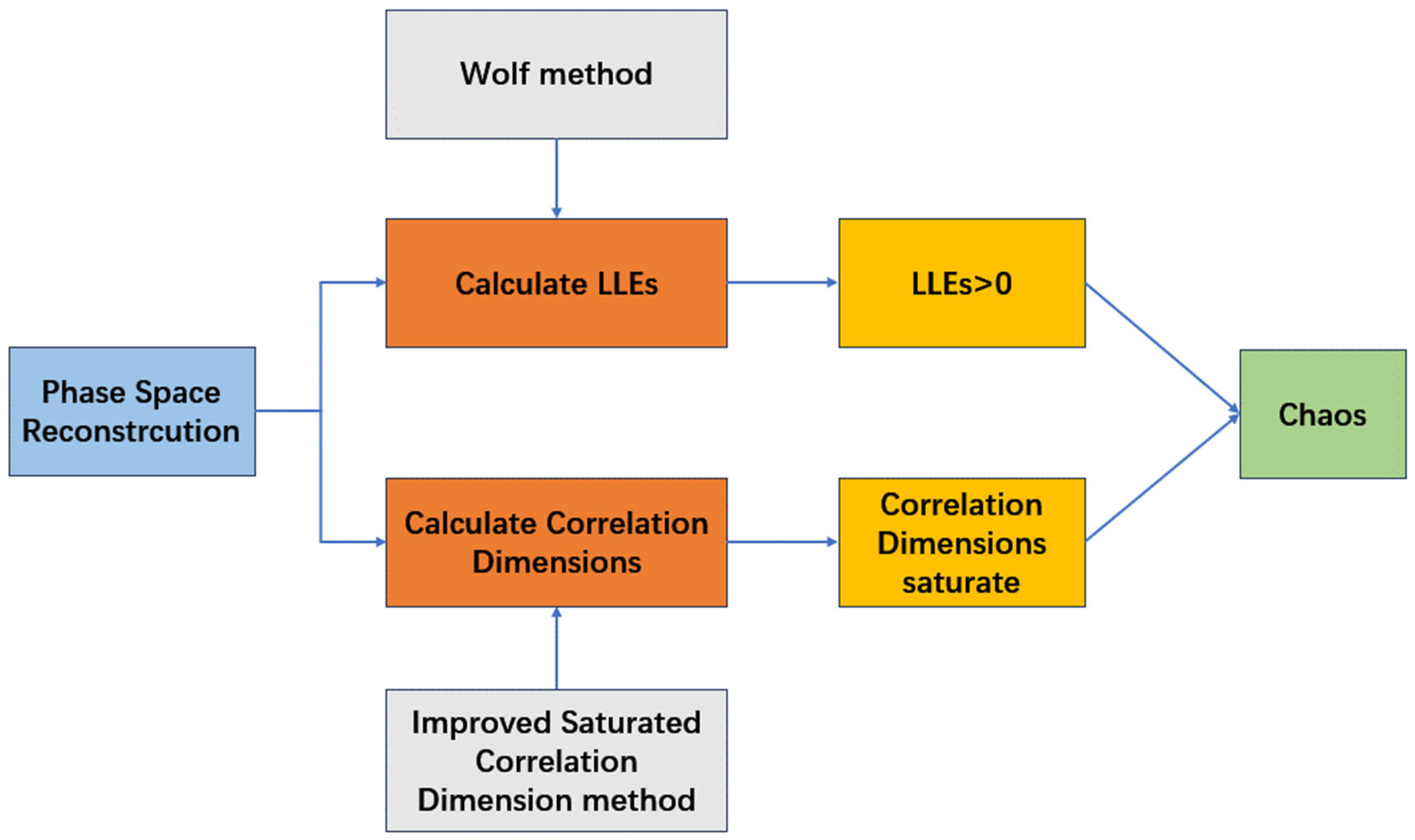
Two methods will be applied to each dataset to analyze its chaotic nature, including the Wolf method and the Improved Saturated Correlation Dimension method. The overall process is shown in Figure 1.

Figure 1.
Analysis process of chaotic nature.
4.1. Analyzing Chaos Using Largest Lyapunov Exponents
The Wolf method for calculating the Largest Lyapunov Exponent (LLE) is a numerical technique used to estimate the separation rate of nearby trajectories in a dynamical system, and it is a method for quantitatively determining the chaotic nature of time series data.
The following sections will use phase space reconstruction and the Wolf method to calculate LLEs for the AGRI China region 4KM L1 data from FY-4A, the AHI full-disk 2KM L1 data from Himawari-8, and the Z500 and T850 data from ERA5. This will allow for a quantitative analysis of their short-term and long-term chaotic properties.
4.1.1. LLEs of FY-4A AGRI 4KM L1 Data
Using the FY-4A Advanced Geostationary Radiation Imager (AGRI) data for the China region at 4KM L1 resolution, the focus is on channel 1 (visible band, central wavelength 0.47 microns), channel 4 (shortwave infrared band, central wavelength 1.375 microns), channel 10 (midwave infrared band, central wavelength 7.1 microns), and channel 13 (longwave infrared band, central wavelength 12.0 microns). These specific channels were selected because they correspond to the visible light, shortwave infrared, midwave infrared, and longwave infrared bands. Channels 1, 4, 10, and 13 are typically used for observing color composite images, cirrus clouds, water vapor, and temperature, respectively. These factors are key drivers of atmospheric dynamics. The combination of these channels can provide a broad perspective of atmospheric processes.
Data were extracted for a 60 × 60 spatial coordinate area, totaling 3600 points, with a spatial resolution of 4 km. For each point, a time series of 90 days with a temporal resolution of 165 times per day was captured, resulting in a sequence with a total length of 14,850. This provided a 60 × 60 × 14,850 three-dimensional spatiotemporal dataset.
Phase space reconstruction is performed on the time series for all coordinate points in this region. The time delay τ and embedding dimension m are calculated using the Autocorrelation method and the False Nearest Neighbors method, respectively, resulting in 60 × 60 matrices of time delays and embedding dimensions. It was found that all m values are equal to 8, but the τ values vary among points. Thus, phase space reconstruction is conducted for each point’s time series based on its corresponding τ and m values using Takens’ theorem. The Wolf method is then employed to calculate the LLEs. LLEs corresponding to each band in this region are shown in Figure 2. The x-axis and y-axis represent the spatial coordinates in the longitude and latitude directions, respectively. If the value at a certain point is greater than 0, it indicates that the LLE at that point is positive. This means that the time series at that location will diverge over time, exhibiting chaotic behavior. When equal to 0, the time series corresponds to quasi-periodic motion or a boundary state in the system, where the behavior is regular but not chaotic. A negative LLE means that the series tends to converge over time, implying that it is stable.
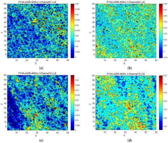
Figure 2.
(a) 60 × 0 LLE diagram of FY-4A AGRI China Area 4KM L1 data for Channel 1; (b) 60 × 60 LLE diagram of FY-4A AGRI China Area 4KM L1 data for Channel 4; (c) 60 × 60 LLE diagram of FY-4A AGRI China Area 4KM L1 data for Channel 10; (d) 60 × 60 LLE diagram of FY-4A AGRI China Area 4KM L1 data for Channel 13.
Using the above method, the data range was extended to cover the entire region and all bands, and the corresponding LLEs were calculated. According to the results, for the FY-4A AGRI China region 4KM L1 data across all bands, more than 99.91% (5,381,233 out of 5,386,080 points, which is the total number of regional points of the data) of the regional points have a corresponding sequence with a positive LLE. Only less than 0.09% of the regional points have a corresponding sequence with a negative LLE. These negative LLEs may result from surface influences such as infrared emission and reflection from the Earth’s surface, terrain-induced atmospheric stability, and boundary layer interactions, which can create localized areas of reduced dynamical complexity and stability in the atmospheric system. On the other hand, negative LLEs may also be attributed to potential numerical artifacts arising from resolution constraints or boundary effects of satellite image. The result above leads to the conclusion that the infrared and visible radiation fields of the atmospheric medium exhibit chaotic nature in the short term.
4.1.2. Himawari-8 AHI 2KM L1 Data
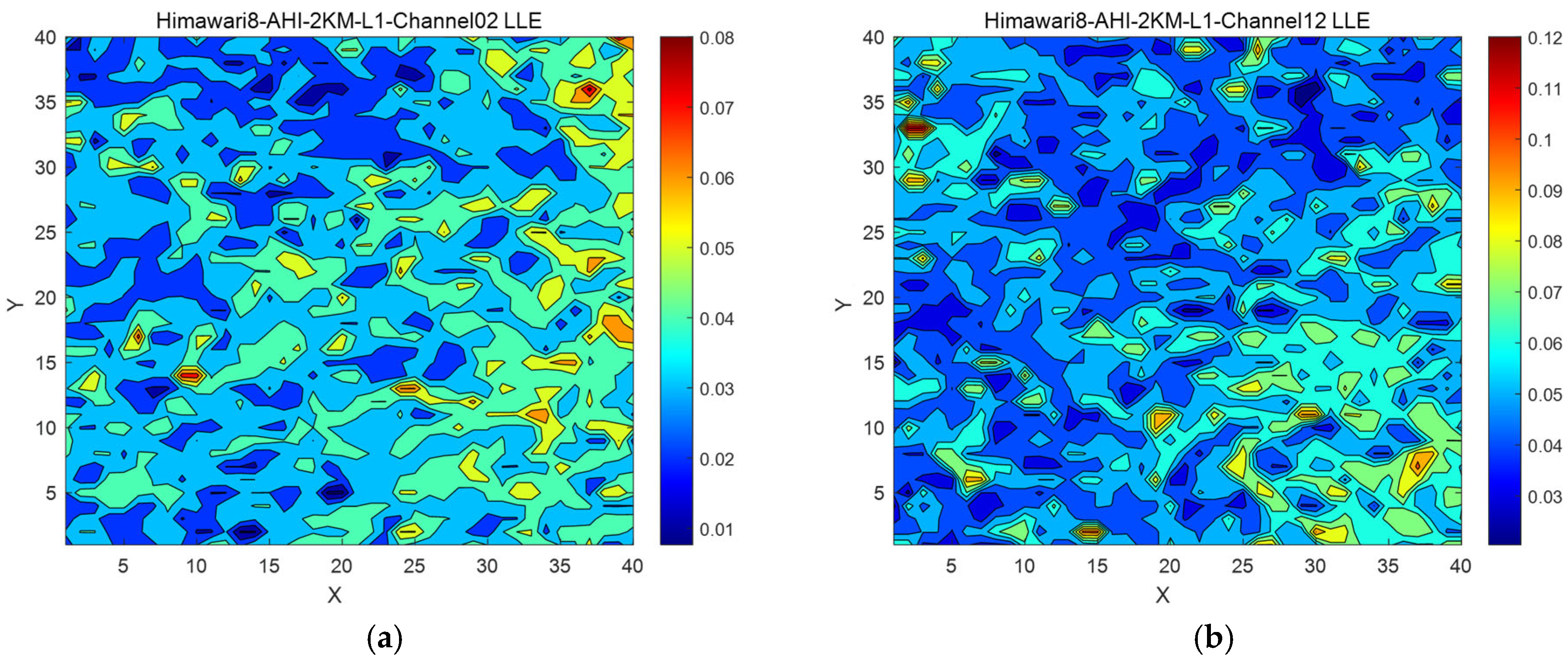
Using the Himawari-8 Advanced Himawari Imager (AHI) full-disk 2KM L1 data for channel 2 (visible band, central wavelength 0.51 microns) and channel 12 (infrared band, central wavelength 9.6 microns) as an example, data were extracted for a 40 × 40 spatial coordinate area, totaling 1600 points [31]. For each point, a time series of 61 days with a temporal resolution of 10 min was captured, resulting in a sequence with a total length of 8784. This provided a 40 × 40 × 8784 three-dimensional spatiotemporal dataset.
Phase space reconstruction is performed on the time series for all coordinate points in this region. The time delay τ and embedding dimension m are calculated using the Autocorrelation method and the False Nearest Neighbors method. The embedding dimensions for all sequences in this region are consistent, with m = 8. The time delays for channel 2 range from 12 to 14, and for channel 12, they range from 30 to 38. Based on the embedding dimensions and the time delays corresponding to each sequence, phase space reconstruction is conducted for all sequences using Takens’ theorem. The Wolf method is then employed to calculate LLEs. LLEs corresponding to each band in this region are shown in Figure 3. The x-axis and y-axis represent the spatial coordinates in the longitude and latitude directions, respectively.
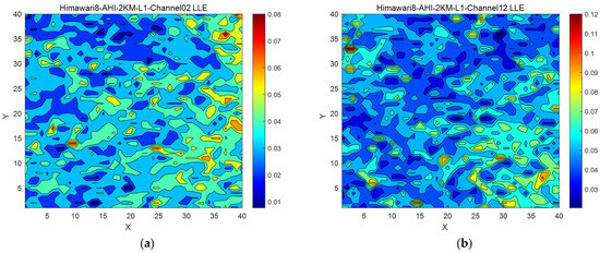
Figure 3.
(a) 40 × 40 LLE diagram of Himawari-8 AHI Full Disk 2KM L1 data for Channel 2; (b) 40 × 40 LLE diagram of Himawari-8 AHI Full Disk 2KM L1 data for Channel 12.
Using the above method, the data range was extended to a global scale and all bands, and the corresponding LLEs were calculated. According to the results, for the Himawari-8 satellite’s AHI full-disk 2KM L1 data across all bands, 99.97% of the regional points have a corresponding sequence with a positive LLE. This leads to the conclusion that the infrared and visible radiation field of the atmospheric medium exhibit chaotic nature in the short term.
4.1.3. ERA5 Z500 and T850 Data
Using the ERA5 reanalysis dataset from the European Centre for Medium-Range Weather Forecasts (ECMWF), specifically the 500 hPa geopotential height data and the 850 hPa temperature data as examples, data were extracted with a spatial resolution of 0.25 degrees. This corresponds to a 41 × 41 grid, covering a 10-degree by 10-degree latitude–longitude area, totaling 1681 points. For each point, a time series from 2015 to 2021 with an hourly resolution was captured, resulting in a total length of 61,368 sequences. This provided a 41 × 41 × 61,368 three-dimensional spatiotemporal dataset.
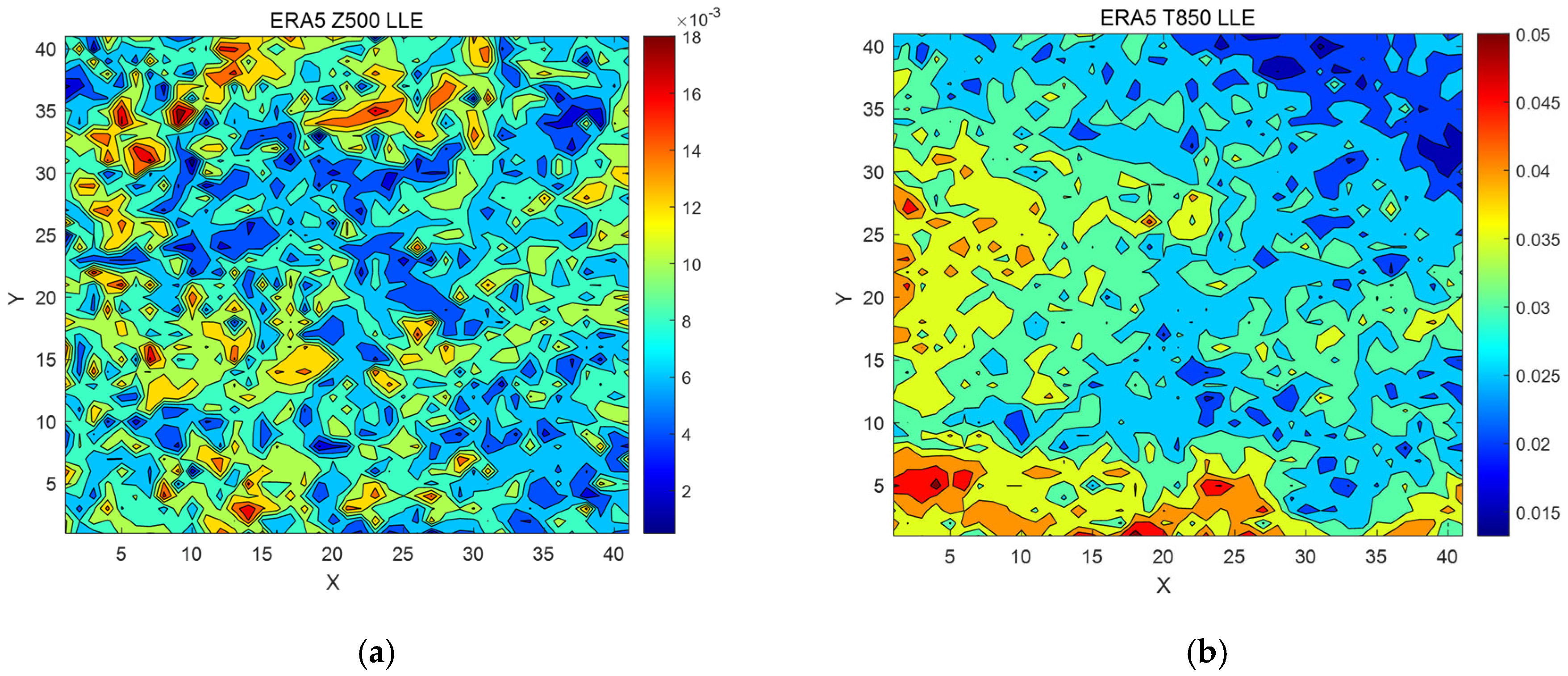
Phase space reconstruction is performed on the time series for all coordinate points in this region. The time delay τ and embedding dimension m are calculated using the autocorrelation method and the false nearest neighbors method. The time delays and embedding dimensions for all sequences in this region are nearly consistent. For Z500 data, τ = 4 and m = 8. For T850 data, τ = 5 and m = 8. Based on these values, phase space reconstruction is conducted for all sequences using Takens’ theorem, and the Wolf method is employed to calculate the LLE. LLEs corresponding to each band in this region are shown in Figure 4.
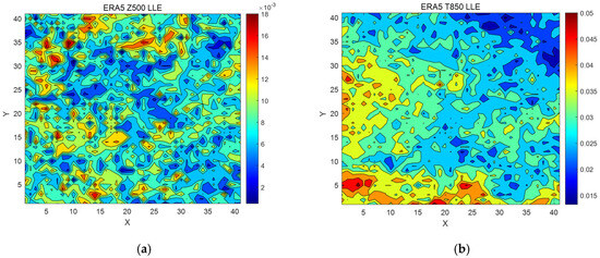
Figure 4.
(a) 41 × 41 LLE diagram of ERA5 hourly data for Z500; (b) 41 × 41 LLE diagram of ERA5 hourly data for T850.
Using the above method, the data range was extended to a global scale, and the corresponding LLEs were calculated. According to the results, for ERA5 Z500 and T850 data, all the points have a corresponding sequence with a positive LLE. This leads to the conclusion that the atmospheric medium exhibits chaotic nature in the long term.
4.2. Analyzing Chaos Using Correlation Dimensions
Using the Improved Saturated Correlation Dimension method described in Section 3.2, the correlation integral for the data in Section 4.1 was calculated and the − curve was plotted. Both the first derivative and the second derivative were calculated to obtain the scaling region. Linear regression was used to calculate the slope in that region, which represents the correlation dimension . By calculating the correlation dimensions corresponding to different embedding dimensions m, the -m curve was obtained. Whether tends to saturate as m increases and the specific value of when saturation occurs, determines whether the sequence is chaotic.
The above method was applied to the FY-4A AGRI 4KM L1, Himawari-8 AHI 2KM L1, ERA5 Z500, and T850 data to analyze the chaotic properties of the atmosphere on both long-term (5 to 10 years) and short-term (2 to 3 months) scales.
4.2.1. Correlation Dimensions of FY-4A AGRI 4KM L1 Data
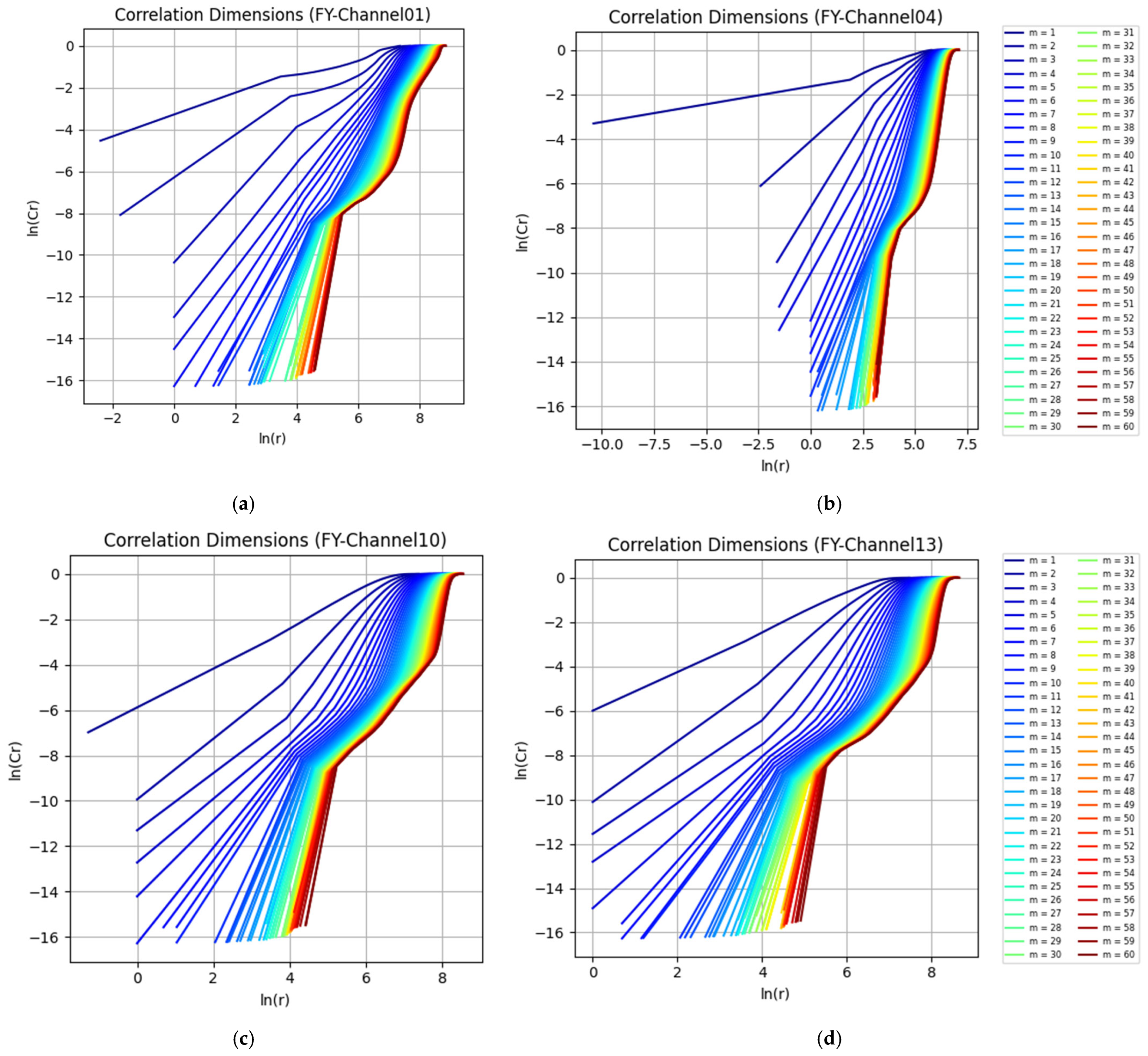
For the FY-4A AGRI China region 4KM L1 data at each grid point in each channel, data were extracted for a time length of 90 days with a temporal resolution of 165 times per day, resulting in a total sequence length of 14,850. Channel 1 (visible band, central wavelength 0.47 microns), channel 4 (shortwave infrared band, central wavelength 1.375 microns), channel 10 (midwave infrared band, central wavelength 7.1 microns), and channel 13 (longwave infrared band, central wavelength 12.0 microns) were taken as examples to calculate the correlation dimensions. Utilizing the G–P method described in 3.2 (see Equations (7) and (8)), the log–log plots of the correlation integral versus the distance for different embedding dimensions m were plotted as Figure 5a–d, corresponding to these 4 channels of FY-4A, respectively. Then, the correlation dimensions were calculated using the curvature-based method proposed in Section 3.2 (see Equations (12) and (14)). The results obtained were largely consistent with the scaling region identified through subjective observation, which validated the feasibility and accuracy of this method. Furthermore, the -m curves of these 4 channels were plotted as Figure 6. From Figure 6, the consistency of the estimated correlation dimension across different embedding dimensions has been verified, which further demonstrated the robustness and accuracy of this curvature-based method.
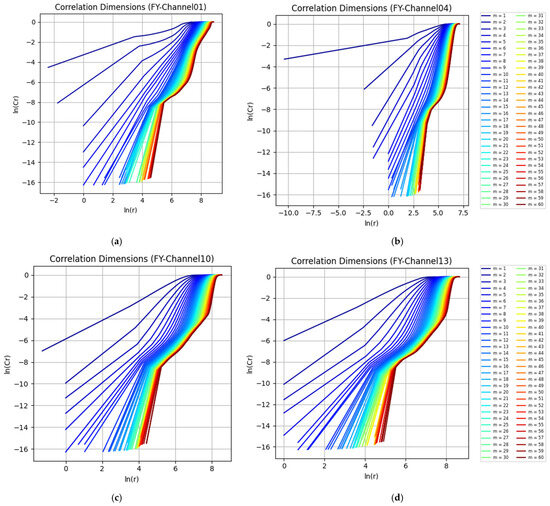
Figure 5.
(a) Log–log plots of the correlation integral versus the distance for different embedding dimensions m for channel 1 of FY-4A AGRI China area 4KM L1 data; (b) Log–log plots of the correlation integral versus the distance for different embedding dimensions m for channel 4 of FY-4A AGRI China area 4KM L1 data; (c) Log–log plots of the correlation integral versus the distance for different embedding dimensions m for channel 10 of FY-4A AGRI China area 4KM L1 data; (d) Log–log plots of the correlation integral versus the distance for different embedding dimensions m for channel 13 of FY-4A AGRI China area 4KM L1 data of FY-4A AGRI China area 4KM L1 data.

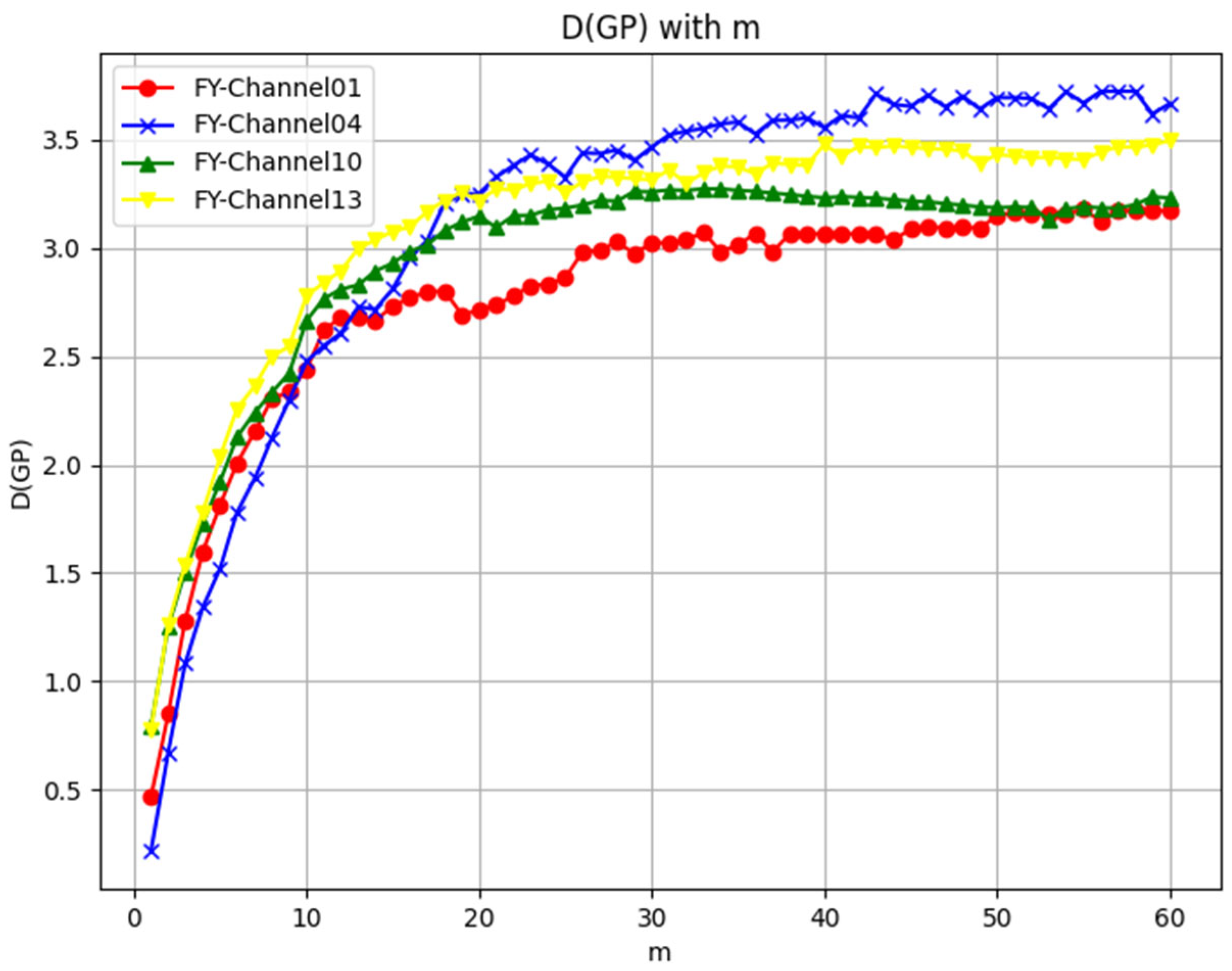
Figure 6.
Correlation Dimension vs. Embedding Dimension Curve for channel 1, channel 4, channel 10 and channel 13 of FY-4A AGRI China area 4KM L1 data.
Finally, the second derivatives of the -m curves were calculated. When the second derivative is smaller than a small threshold, it indicates that the correlation dimension is approaching saturation. Here, the threshold was set to 0.1. From Figure 6, it can be observed that the correlation dimensions for channels 1, 4, 10, and 13 tend to saturate at approximately 3.2, 3.7, 3.2 and 3.5, respectively, as the embedding dimension increases. This saturation indicates that the sequences exhibit chaotic nature. Similarly, the correlation dimensions calculated for data from each channel and each grid point ultimately saturated at dimensions greater than 1 as the embedding dimension increases, proving that the FY-4A AGRI 4KM L1 data exhibits chaotic nature on a short-term scale.
4.2.2. Correlation Dimensions of Himawari-8 AHI 2KM L1 Data
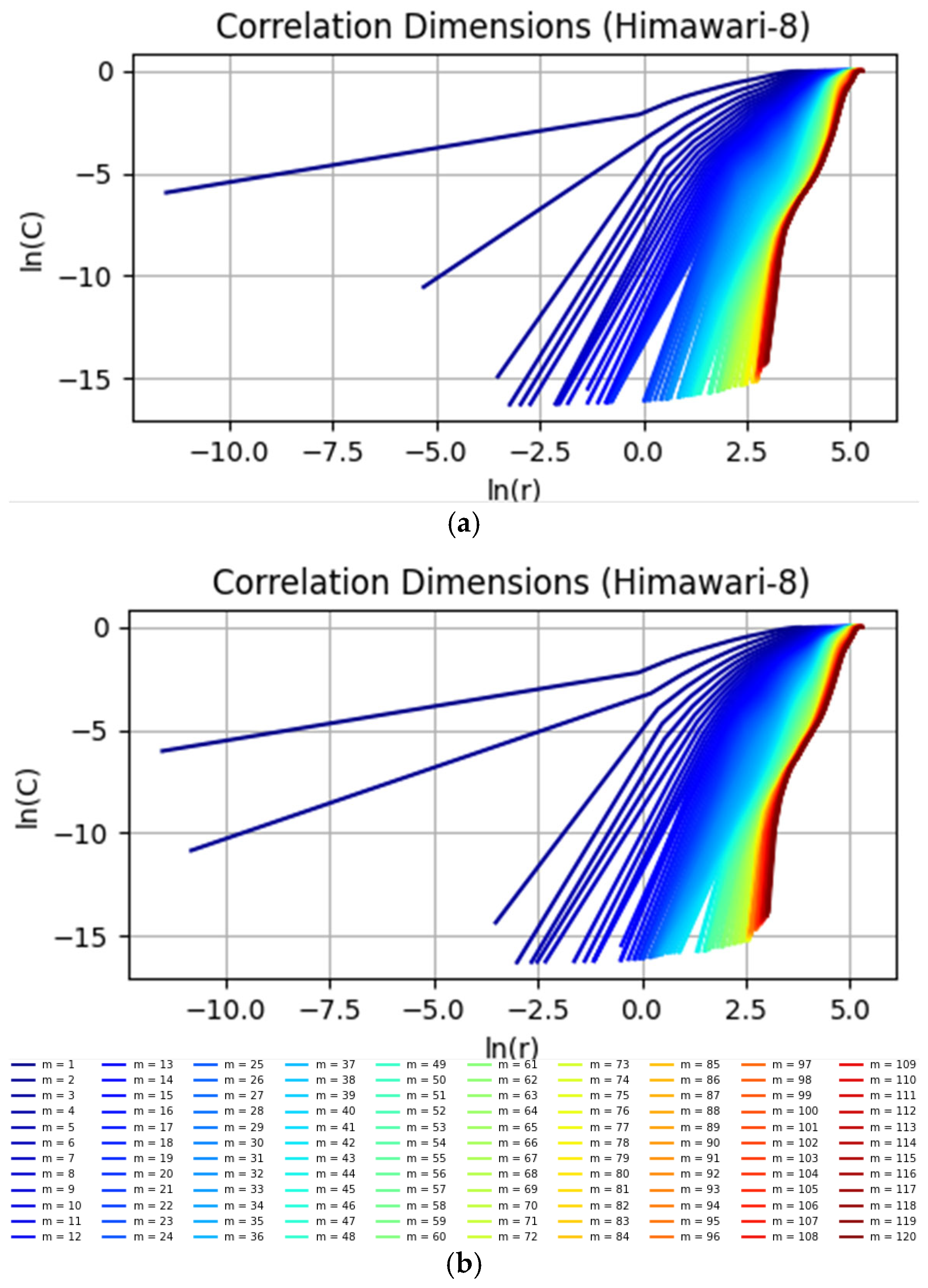
For the Himawari-8 AHI full-disk 2KM L1 data at each grid point in each channel, data were extracted for a time length of 61 days with a temporal resolution of 10 min, resulting in a total sequence length of 8784. Grid point at coordinates (4050, 5250) (approximately 20.98°S, 175.02°W) from channel 2 (visible band, central wavelength 0.51 microns) and channel 12 (infrared band, central wavelength 9.6 microns) were taken as examples to calculate the correlation dimensions. Utilizing the G–P method described in 3.2 (see Equations (7) and (8)), the log–log plots of the correlation integral versus the distance for different embedding dimensions m were plotted as Figure 7a,b, corresponding to these 2 channels of Himawari-8, respectively. Then, the correlation dimensions were calculated using the curvature-based method proposed in 3.2 (see Equations (12) and (14)). The results obtained were largely consistent with the scaling region identified through subjective observation. The -m curves were plotted as Figure 8. The consistency of the estimated correlation dimension across different embedding dimensions has been verified in Figure 8, which further demonstrated the feasibility and accuracy of this curvature-based method.

Figure 7.
(a) Log–log plots of the correlation integral versus the distance for different embedding dimensions m for channel 2 of Himawari-8 AHI full-disk 2KM L1 data; (b) Log–log plots of the correlation integral versus the distance for different embedding dimensions m for channel 12 of Himawari-8 AHI full-disk 2KM L1 data.

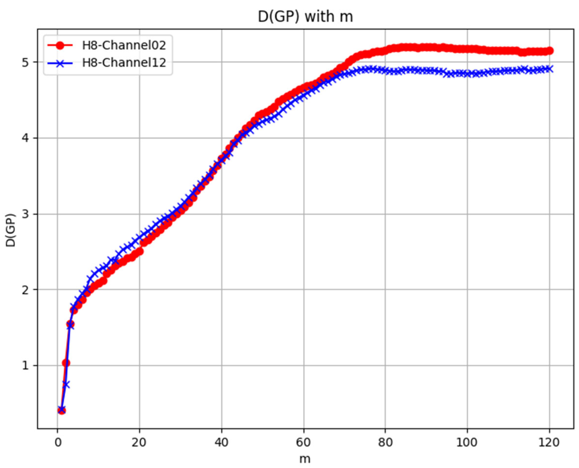
Figure 8.
Correlation Dimension vs. Embedding Dimension Curve for channel 2 and channel 12 of Himawari-8 AHI Full disk 2KM L1 data at location (4050, 5250).
From Figure 8, it can be observed that the correlation dimensions for channel 2 and 12 tended to saturate at approximately 5.1 and 4.9, respectively, where the second derivatives of the -m curves were smaller than the threshold 0.1. This saturation indicates that the sequences exhibit chaotic nature. Similarly, the correlation dimensions calculated for data from each channel and each grid point ultimately saturated at dimensions greater than 1 as the embedding dimension increases, proving that the Himawari-8 AHI full-disk 2KM L1 data exhibits chaotic nature on a short-term scale.
4.2.3. Correlation Dimensions of ERA5 Z500 and T850 Data
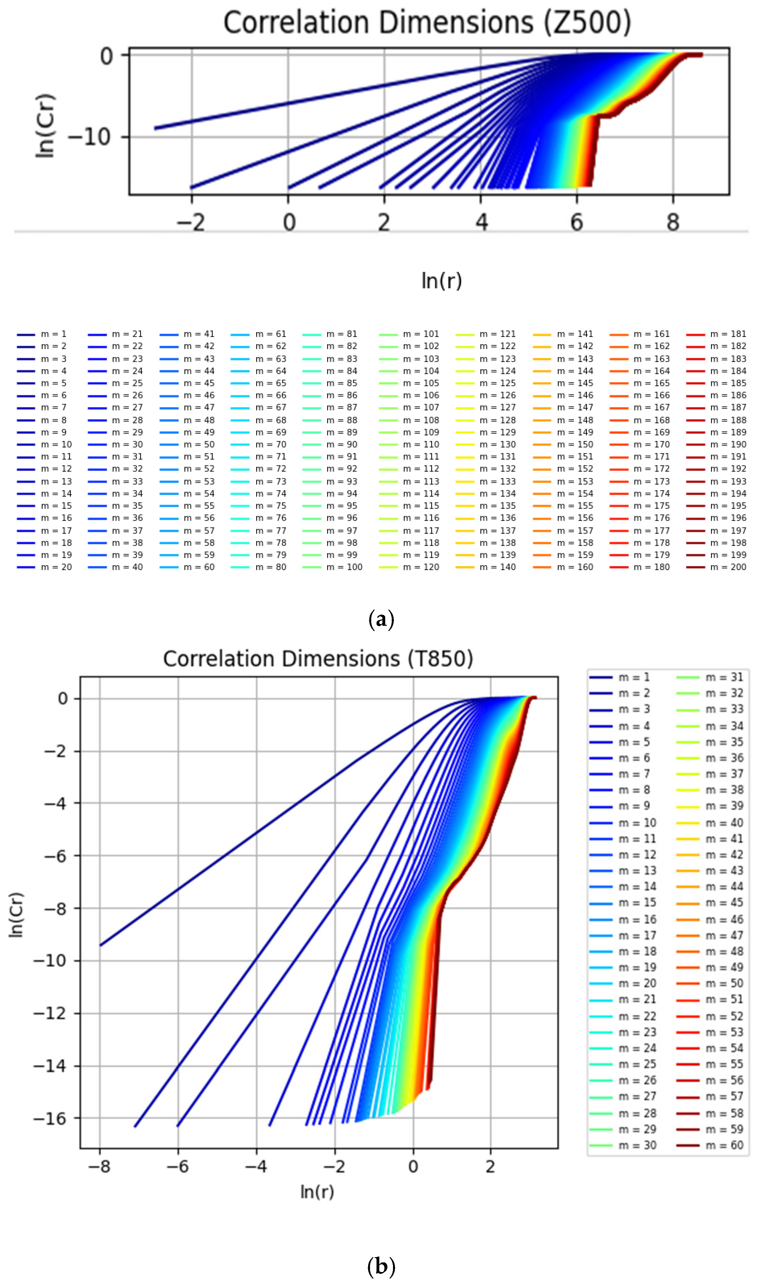
For the ERA5 reanalysis dataset from European Centre for Medium-Range Weather Forecasts (ECMWF), specifically the 500 hPa geopotential height data and the 850 hPa temperature data, data were extracted for the period from 2015 to 2021 with an hourly resolution, resulting in a total sequence length of 61,368. Utilizing the G–P method, described in Section 3.2 (see Equations (7) and (8)), the log–log plots of the correlation integral versus the distance for different embedding dimensions m were plotted as Figure 9a,b, corresponding to Z500 and T850 hourly data of ERA5 at 20.00°S, 175.00°W, respectively. Then, the correlation dimensions were calculated using the curvature-based method proposed in Section 3.2 (see Equations (12) and (14)). The -m curves were plotted as Figure 10. The scaling regions obtained were largely consistent with those identified through subjective observation. And the consistency of the estimated correlation dimension across different embedding dimensions has been verified in Figure 10, which demonstrated the feasibility and accuracy of this curvature-based method.
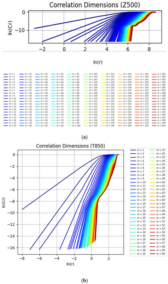
Figure 9.
(a) Log–log plots of the correlation integral versus the distance for different embedding dimensions m for Z500 hourly data of ERA5 at 20.00°S, 175.00°W; (b) Log–log plots of the correlation integral versus the distance for different embedding dimensions m for T850 hourly data of ERA5 at 20.00°S, 175.00°W.
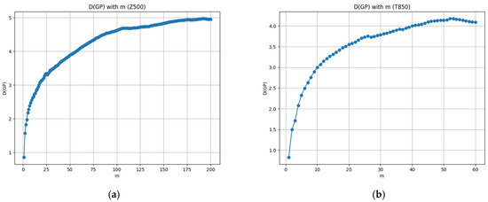
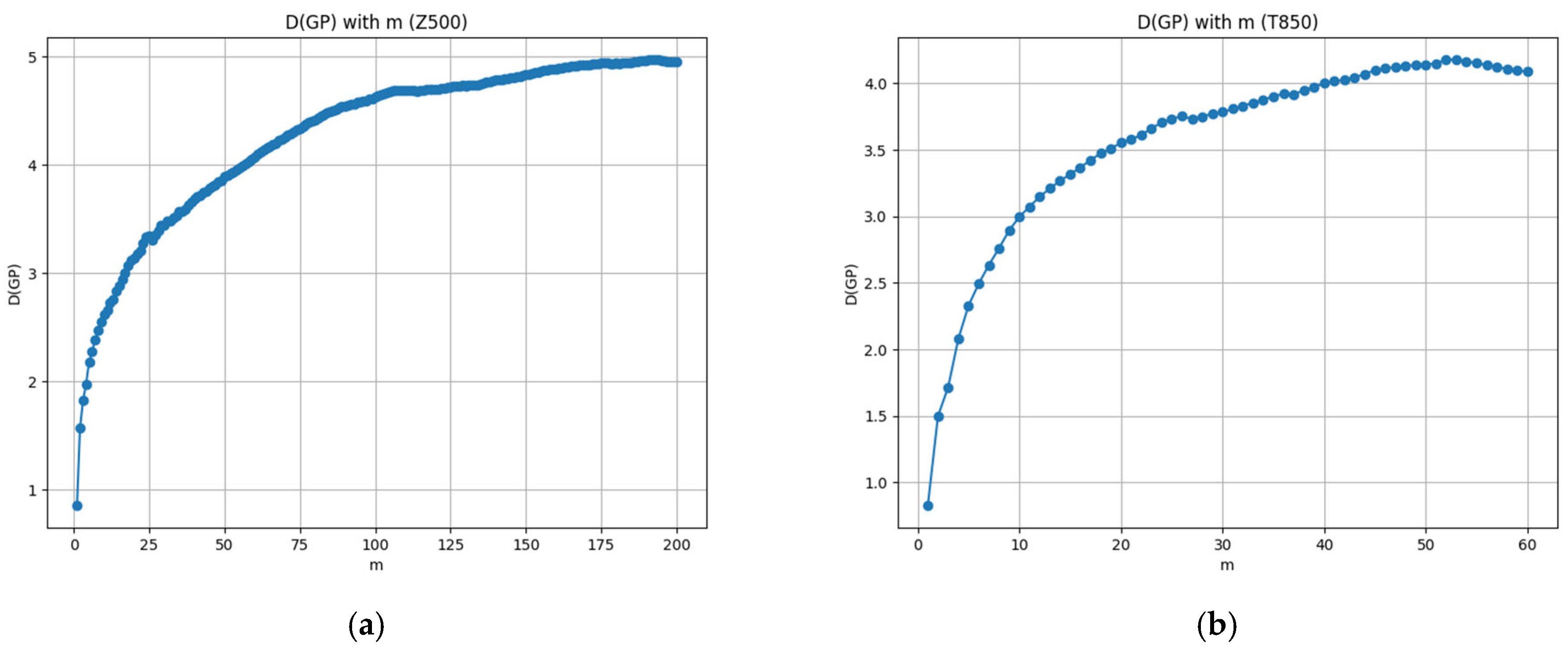
Figure 10.
(a) Correlation Dimension vs. Embedding Dimension Curve for Z500 hourly data of ERA5 at 20.00°S, 175.00°W; (b) Correlation Dimension vs. Embedding Dimension Curve for T850 hourly data of ERA5 at 20.00°S, 175.00°W.
The correlation dimensions for the Z500 and T850 sequences tended to saturate at approximately 4.95 and 4.05, respectively, as the embedding dimension increases, demonstrating the chaotic nature of these sequences. Similarly, the correlation dimensions calculated for sequences at each latitude and longitude point ultimately saturate at dimensions greater than 1 as the embedding dimension increases, proving that the ERA5 Z500 and T850 hourly data exhibit chaotic nature on a long-term scale.
5. Conclusions
In this paper, an overview of the definition and characteristics of chaos was provided. Phase space reconstruction, as a crucial preprocessing method for chaotic data, was introduced. And two quantitative methods for determining chaotic nature were thoroughly discussed. The first was the Lyapunov Exponent method, and the second was the Improved Saturated Correlation Dimension method, which was newly proposed in this work. This new method, based on curvature and the least squares approach, effectively addressed the subjectivity and noise sensitivity issues in determining the scaling region of the − curves associated with the traditional G–P method. On this basis, this paper innovatively applies the above two methods to satellite remote-sensing L1 datasets including FY-4A and Himawari-8, as well as ERA5 reanalysis dataset. Two indicators were analyzed: whether the system’s Largest Lyapunov Exponent is positive and whether the correlation dimension tends to saturate with the embedding dimension. The results showed that, on the one hand, the overwhelming majority of sequences of satellite remote-sensing L1 dataset (99.91% for FY-4A and 99.97% for Himawari-8) and all the sequences of ERA5 have positive LLEs. Considering the surface influences from the Earth’s surface, and boundary layer interactions, which may result in the negative LLEs of less than 0.01%, the results obtained from the more comprehensive ERA5 dataset can be considered reliable. On the other hand, all the sequences of both satellite remote-sensing L1 dataset and ERA5 dataset have correlation dimensions saturating at values greater than 1. Taking into account the above two indicators comprehensively, the following conclusion can be drawn: on both short-term and long-term scales, the atmospheric medium exhibits chaotic nature.
In summary, this paper demonstrated the chaotic behavior of the atmospheric system on different scales, which helps to reveal the multi-scale interactions and coupling mechanisms of the atmospheric system. This provides an experimental basis for a deeper understanding of the highly complex internal structure and dynamic evolution mechanisms of the atmospheric system. On this basis, the characteristics of chaotic systems can be utilized in the future to study the evolution of variables in the atmospheric system using numerical integration and data-driven methods, further improving the accuracy of weather forecasts. Additionally, early warning and prediction of natural disasters such as volcanic eruptions and typhoons can be conducted based on minute abnormal disturbances in the atmospheric medium. On the other hand, the sensitivity to initial conditions in chaos can be used to capture weak moving targets under the atmospheric infrared background radiation field, which is of great significance for improving the detection rate of hostile targets in military confrontations.
Author Contributions
Conceptualization, Z.W. and W.X.; methodology, Z.W. and S.S.; software, Z.W.; validation, Z.W.; formal analysis, Z.W. and W.X.; investigation, Z.W., W.X., R.C. and Y.M.; resources, Z.W. and G.L.; data curation, Z.W. and W.X.; writing—original draft preparation, Z.W.; writing—review and editing, Z.W.; visualization, Z.W.; supervision, S.S. and W.X.; project administration, S.S. All authors have read and agreed to the published version of the manuscript.
Funding
This research received no external funding.
Data Availability Statement
The original data presented in the study are openly available in ERA5 at https://cds.climate.copernicus.eu, FY-4A at https://satellite.nsmc.org.cn/portalsite/default.aspx and Himawari-8 at https://www.eorc.jaxa.jp/ptree/index.html (accessed on 8 September 2024).
Acknowledgments
The authors would like to thank the members of Key Laboratory of Intelligent Infrared Sensing, Chinese Academy of Sciences, for their substantial support on hardware.
Conflicts of Interest
The authors declare no conflict of interest.
References
- Lyapunov, A.M. The general problem of the stability of motion. Int. J. Control. 1992, 55, 531–534. [Google Scholar] [CrossRef]
- Poincaré, H. New Methods of Celestial Mechanics; National Aeronautics and Space Administration: Washington, DC, USA, 1967. [Google Scholar]
- Van der Pol, B.; Van Der Mark, J. Frequency demultiplication. Nature 1927, 120, 363–364. [Google Scholar] [CrossRef]
- Lorenz, E.N. Deterministic nonperiodic flow. J. Atmos. Sci. 1963, 20, 130–141. [Google Scholar] [CrossRef]
- Smale, S. Differentiable dynamical systems. Bull. Am. Math. Soc. 1967, 73, 747–817. [Google Scholar] [CrossRef]
- Li, T.Y.; Yorke, J.A. Period Three Implies Chaos. Am. Math. Mon. 1975, 82, 985. [Google Scholar] [CrossRef]
- Feigenbaum, M.J. Quantitative universality for a class of nonlinear transformations. J. Stat. Phys. 1978, 19, 25–52. [Google Scholar] [CrossRef]
- May, R.M. Simple mathematical models with very complicated dynamics. Nature 1976, 261, 459–467. [Google Scholar] [CrossRef]
- Takens, F. Detecting strange attractors in turbulence. In Dynamical Systems and Turbulence, Warwick 1980: Proceedings of a Symposium Held at the University of Warwick, 1979/80; Springer: Berlin/Heidelberg, Germany, 2006. [Google Scholar]
- Mandelbrot, B.B. The Fractal Geometry of Nature; WH Freeman: New York, NY, USA, 1982; Volume 1. [Google Scholar]
- Grassberger, P.; Procaccia, I. Measuring the strangeness of strange attractors. Phys. D Nonlinear Phenom. 1983, 9, 189–208. [Google Scholar] [CrossRef]
- Shaw, J.A.; Nugent, P.W. Physics principles in radiometric infrared imaging of clouds in the atmosphere. Eur. J. Phys. 2013, 34, S111. [Google Scholar] [CrossRef]
- Hersbach, H.; Bell, B.; Berrisford, P.; Hirahara, S.; Horányi, A.; Muñoz-Sabater, J.; Nicolas, J.; Peubey, C.; Radu, R.; Schepers, D.; et al. The ERA5 global reanalysis. Q. J. R. Meteorol.Soc. 2020, 146, 1999–2049. [Google Scholar] [CrossRef]
- Tsonis, A.A. Chaos: From Theory to Applications; Springer Science & Business Media: Berlin/Heidelberg, Germany, 2012. [Google Scholar]
- Kennel, M.B.; Brown, R.; Abarbanel, H.D. Determining embedding dimension for phase-space reconstruction using a geometrical construction. Phys. Rev. A 1992, 45, 3403. [Google Scholar] [CrossRef] [PubMed]
- Buzug, T.; Pfister, G. Comparison of algorithms calculating optimal embedding parameters for delay time coordinates. Phys. D Nonlinear Phenom. 1992, 58, 127–137. [Google Scholar] [CrossRef]
- Rhodes, C.; Morari, M. The false nearest neighbors algorithm: An overview. Comput. Chem. Eng. 1997, 21, S1149–S1154. [Google Scholar] [CrossRef]
- Kim, H.S.; Eykholt, R.; Salas, J. Nonlinear dynamics, delay times, and embedding windows. Phys. D Nonlinear Phenom. 1999, 127, 48–60. [Google Scholar] [CrossRef]
- Abarbanel, H.D.; Kennel, M.B. Local false nearest neighbors and dynamical dimensions from observed chaotic data. Phys. Rev. E 1993, 47, 3057. [Google Scholar] [CrossRef]
- Fraser, A.M. Information and entropy in strange attractors. IEEE Trans. Inf. Theory 1989, 35, 245–262. [Google Scholar] [CrossRef]
- Ott, E. Chaos in Dynamical Systems; Cambridge University Press: Cambridge, UK, 2002. [Google Scholar]
- Wolf, A.; Swift, J.B.; Swinney, H.L.; Vastano, J.A. Determining Lyapunov exponents from a time series. Phys. D Nonlinear Phenom. 1985, 16, 285–317. [Google Scholar] [CrossRef]
- Sandri, M. Numerical calculation of Lyapunov exponents. Math. J. 1996, 6, 78–84. [Google Scholar]
- Benettin, G.; Galgani, L.; Giorgilli, A.; Strelcyn, J.-M. Lyapunov characteristic exponents for smooth dynamical systems and for Hamiltonian systems; a method for computing all of them. Part 1: Theory. Meccanica 1980, 15, 9–20. [Google Scholar] [CrossRef]
- Grassberger, P.; Procaccia, I. Characterization of strange attractors. Phys. Rev. Lett. 1983, 50, 346. [Google Scholar] [CrossRef]
- Simpelaere, D. Correlation dimension. J. Stat. Phys. 1998, 90, 491–509. [Google Scholar] [CrossRef]
- Bradley, E.; Kantz, H. Nonlinear time-series analysis revisited. Chaos Interdiscip. J. Nonlinear Sci. 2015, 25, 097610. [Google Scholar] [CrossRef] [PubMed]
- Theiler, J. Estimating fractal dimension. JOSA A 1990, 7, 1055–1073. [Google Scholar] [CrossRef]
- Kantz, H.; Schreiber, T. Nonlinear Time Series Analysis; Cambridge University Press: Cambridge, UK, 2004; Volume 7. [Google Scholar]
- Eckmann, J.-P.; Ruelle, D. Ergodic theory of chaos and strange attractors. Rev. Mod. Phys. 1985, 57, 617. [Google Scholar] [CrossRef]
- Bessho, K.; Hayashi, M.; Ikeda, A.; Imai, T.; Inoue, H.; Kumagai, Y.; Miyakawa, T.; Murata, H.; Ohno, T.; Okuyama, A. An introduction to Himawari-8/9—Japan’s new-generation geostationary meteorological satellites. J. Meteorol. Soc. Japan. Ser. II 2016, 94, 151–183. [Google Scholar] [CrossRef]

Disclaimer/Publisher’s Note: The statements, opinions and data contained in all publications are solely those of the individual author(s) and contributor(s) and not of MDPI and/or the editor(s). MDPI and/or the editor(s) disclaim responsibility for any injury to people or property resulting from any ideas, methods, instructions or products referred to in the content. |
© 2024 by the authors. Licensee MDPI, Basel, Switzerland. This article is an open access article distributed under the terms and conditions of the Creative Commons Attribution (CC BY) license (https://creativecommons.org/licenses/by/4.0/).