
Thorough Understanding and 3D Super-Resolution Imaging for Forward-Looking Missile-Borne SAR via a Maneuvering Trajectory


Abstract
:1. Introduction
2. The Understanding of Maneuvering Trajectory for Three-Dimensional and Forward-Looking Missile-Borne SAR
3. Three-Dimensional Super-Resolution Imaging Combining Axis Rotation and Compressed Sensing
4. Simulation and Results
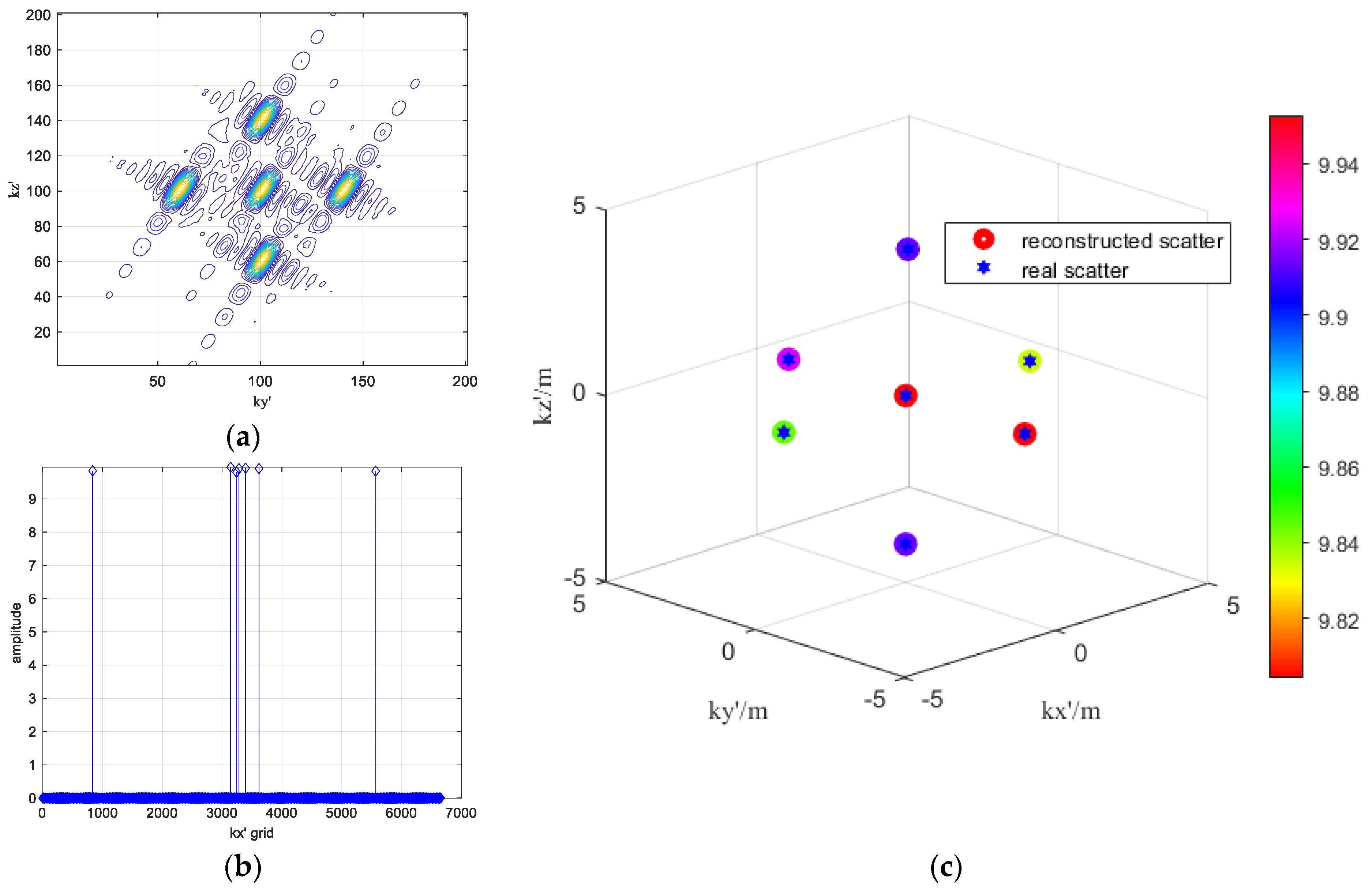
4.1. 3D Imaging for Multi-Scatters with the Same and Varying Reflection Coefficients
4.2. Effects of the Signal-to-Noise Ratio and Sampling Rate on 3D Imaging Processing
4.3. 3D Imaging Verification with the Point Cloud Models of Actual Complex Tank Object
5. Conclusions
Author Contributions
Funding
Data Availability Statement
Conflicts of Interest
References
- Cumming, I.G.; Wong, F.H. Digital Processing of Synthetic Aperture Radar Data: Algorithm and Implementation; Artech House: Norwood, MA, USA, 2005. [Google Scholar]
- Moreira, A.; Prats-Iraola, P.; Younis, M.; Krieger, G.; Hajnsek, I.; Papathanassiou, K.P. A tutorial on synthetic aperture radar. IEEE Geosci. Remote Sens. Mag. 2013, 1, 563–583. [Google Scholar] [CrossRef]
- Chen, X.; Sun, G.-C.; Xing, M.; Li, B.; Yang, J.; Bao, Z. Ground Cartesian back-projection algorithm for high squint diving Tops SAR imaging. IEEE Trans. Geosci. Remote Sens. 2021, 59, 5812–5827. [Google Scholar] [CrossRef]
- Deng, Y.; Sun, G.-C.; Han, L.; Wang, Y.; Zhang, Y.; Xing, M. 2-D Wavenumber Domain Autofocusing for High-Resolution Highly Squinted SAR Imaging Based on Equivalent Broadside Model. IEEE Trans. Geosci. Remote Sens. 2023, 61, 5220515. [Google Scholar] [CrossRef]
- Xu, H.P.; Zhu, Y.D.; Kang, C.H.; Zhou, Y.Q. A new deramp NECS imaging algorithm for missile borne hybrid SAR. Chin. J. Electron. 2011, 20, 769–774. [Google Scholar]
- Liu, D.; Shi, H.; Liu, H.; Yang, T.; Guo, J. Enhanced Forward-Looking Missile-Borne Bistatic SAR Imaging with Electromagnetic Vortex. IEEE Sens. J. 2023, 23, 8478–8490. [Google Scholar] [CrossRef]
- Qian, G.; Wang, Y. Analysis of Modeling and 2-D Resolution of Satellite–Missile Borne Bistatic Forward-Looking SAR. IEEE Trans. Geosci. Remote Sens. 2023, 61, 5222314. [Google Scholar] [CrossRef]
- Li, X.; Zhou, S.; Yang, L. A new fast factorized back-projection algorithm with reduced topography sensibility for missile-borne SAR focusing with diving movement. Remote Sens. 2020, 12, 2616. [Google Scholar] [CrossRef]
- Wang, C.; Sun, H.; Zhang, X.-Y.; Zhang, R. A unified back-projection correction algorithm for squint SAR based on SPECAN processing. In Proceedings of the 2019 IEEE International Conference on Signal, Information and Data Processing (ICSIDP), Chongqing, China, 11–13 December 2019; pp. 1–4. [Google Scholar]
- Tang, S.; Zhang, L.; Guo, P.; Zhao, Y. An omega-K algorithm for highly squinted missile-borne SAR with constant acceleration. IEEE Geosci. Remote Sens. Lett. 2014, 11, 1569–1573. [Google Scholar] [CrossRef]
- Chen, S.; Zhao, H.; Zhang, S.; Chen, Y. An extended nonlinear chirp scaling algorithm for missile borne SAR imaging. Signal Process. 2014, 99, 58–68. [Google Scholar] [CrossRef]
- Li, Z.; Xing, M.; Liang, Y.; Gao, Y.; Chen, J.; Huai, Y.; Zeng, L.; Sun, G.C.; Bao, Z. A frequency-domain imaging algorithm for highly squinted SAR mounted on maneuvering platforms with nonlinear trajectory. IEEE Trans. Geosci. Remote Sens. 2016, 54, 4023–4038. [Google Scholar] [CrossRef]
- Zhang, Y.; Lu, C.; Zhang, H.; Li, H. A Modified CSA for Missile-Borne SAR with Curved Trajectory. In Proceedings of the 2020 IEEE Radar Conference (RadarConf20), Florence, Italy, 21–25 September 2020; pp. 1–6. [Google Scholar]
- Saeedi, J. Feasibility study and conceptual design of missile-borne synthetic aperture radar. IEEE Trans. Syst. Man Cybern. Syst. 2020, 50, 1122–1133. [Google Scholar] [CrossRef]
- Zhu, D.; Xiang, T.; Wei, W.; Ren, Z.; Yang, M.; Zhang, Y.; Zhu, Z. An extended two step approach to high-resolution airborne and spaceborne SAR full-aperture processing. IEEE Trans. Geosci. Remote Sens. 2021, 59, 8382–8397. [Google Scholar] [CrossRef]
- Tang, S.; Zhang, X.; He, Z.; Chen, Z. Practical Issue Analyses and Imaging Approach for Hypersonic Vehicle-Borne SAR with Near-Vertical Diving Trajectory. IEEE Trans. Geosci. Remote Sens. 2023, 61, 5204316. [Google Scholar] [CrossRef]
- Dong, L.; Han, S.; Zhu, D.; Mao, X. A Modified Polar Format Algorithm for Highly Squinted Missile-Borne SAR. IEEE Geosci. Remote Sens. Lett. 2023, 20, 4012905. [Google Scholar] [CrossRef]
- Zheng, Y.; Guan, J.; Jiang, G.; Yi, W.; Yang, X.; Yin, H. A Modified Algorithm for Highly Squinted Missile-Borne SAR Imaging with Large Acceleration. IEEE Access 2024, 12, 48640–48653. [Google Scholar] [CrossRef]
- Zebker, H.; Goldstein, R. Topographic mapping from interferometric SAR observations. J. Geophys. Res. 1986, 91, 4993–4999. [Google Scholar] [CrossRef]
- Zhu, X.; Bamler, R. Tomographic SAR inversion by L1-norm regularization—The compressive sensing approach. IEEE Trans. Geosci. Remote Sens. 2010, 48, 3839–3846. [Google Scholar] [CrossRef]
- Bi, H.; Zhang, B.; Hong, W.; Zhou, S. Matrix-Completion-Based Airborne Tomographic SAR Inversion under Missing Data. IEEE Geosci. Remote Sens. Lett. 2015, 12, 2346–2350. [Google Scholar] [CrossRef]
- Reale, D.; Fornaro, G.; Pauciullo, A.; Zhu, X.; Bamler, R. Tomographic imaging and monitoring of buildings with very high resolution SAR data. IEEE Geosci. Remote Sens. Lett. 2011, 8, 661–665. [Google Scholar] [CrossRef]
- Gu, T.; Liao, G.; Li, Y.; Liu, Y.; Guo, Y. Airborne Downward-Looking Sparse Linear Array 3-D SAR Imaging via 2-D Adaptive Iterative Reweighted Atomic Norm Minimization. IEEE Trans. Geosci. Remote Sens. 2022, 60, 5202513. [Google Scholar] [CrossRef]
- Gu, T.; Liao, G.; Li, Y.; Guo, Y.; Liu, Y. DLSLA 3-D SAR Imaging via Sparse Recovery through Combination of Nuclear Norm and Low-Rank Matrix Factorization. IEEE Trans. Geosci. Remote Sens. 2022, 60, 5208213. [Google Scholar] [CrossRef]
- Shao, M.; Su, C.; Zhang, Z.; Zhang, B. The application of the alternate descent conditional gradient method in tomographic SAR off-grid imaging. In Proceedings of the IET International Radar Conference (IRC 2023), Chongqing, China, 3–5 December 2023; pp. 3259–3264. [Google Scholar]
- Tian, W.; Xie, X.; Deng, Y.; Yang, Z.; Hu, C. An Improved Imaging Method Based on Optimal Topographic Imaging Plane Reconstruction for Nonlinear Trajectory SAR. IEEE Trans. Geosci. Remote Sens. 2024, 62, 5216217. [Google Scholar] [CrossRef]
- Meng, D.; Hu, D.; Ding, C. A New Approach to Airborne High Resolution SAR Motion Compensation for Large Trajectory Deviations. Chin. J. Electron. 2012, 21, 764–769. [Google Scholar]
- Gorovyi, I.M.; Bezvesilniy, O.O.; Vavriv, D.M. Estimation of uncompensated trajectory deviations and image refocusing for high-resolution SAR. In Proceedings of the 2015 German Microwave Conference, Nuremberg, Germany, 16–18 March 2015; pp. 186–189. [Google Scholar]
- Ran, L.; Liu, Z.; Zhang, T.; Li, T. Autofocus for correcting three dimensional trajectory deviations in synthetic aperture radar. In Proceedings of the 2016 CIE International Conference on Radar (RADAR), Guangzhou, China, 10–13 October 2016; pp. 1–4. [Google Scholar]
- Ran, L.; Liu, Z.; Zhang, L.; Li, T.; Xie, R. An Autofocus Algorithm for Estimating Residual Trajectory Deviations in Synthetic Aperture Radar. IEEE Trans. Geosci. Remote Sens. 2017, 55, 3408–3425. [Google Scholar] [CrossRef]
- Liu, Y.; Wang, W.; Pan, X.; Gu, Z.; Wang, G. Raw Signal Simulator for SAR with Trajectory Deviation Based on Spatial Spectrum Analysis. IEEE Trans. Geosci. Remote Sens. 2017, 55, 6651–6665. [Google Scholar] [CrossRef]
- An, Z.; Xiong, F.; Li, C. A Trajectory Tracking Method Using Convex Optimization. In Proceedings of the 2020 39th Chinese Control Conference (CCC), Shenyang, China, 27–29 July 2020; pp. 3281–3287. [Google Scholar]
- Chen, X.; Li, Z.; Yang, Y.; Qi, L.; Ke, R. High-Resolution Vehicle Trajectory Extraction and Denoising from Aerial Videos. IEEE Trans. Intell. Transp. Syst. 2021, 22, 3190–3202. [Google Scholar] [CrossRef]
- Donoho, D.L. Compressed sensing. IEEE Trans. Theory 2006, 52, 1289–1306. [Google Scholar] [CrossRef]
- Kim, S.-J.; Koh, K.; Lustig, M.; Boyd, S.; Gorinevsky, D. An Interior-Point Method for Large-Scale ℓ -Regularized Least Squares. IEEE J. Sel. Top. Signal Process. 2007, 1, 606–617. [Google Scholar] [CrossRef]
- Austin, C.D.; Ertin, E.; Moses, R.L. Sparse signal methods for 3D radar imaging. IEEE J. Sel. Topics Signal Process. 2011, 5, 408–423. [Google Scholar] [CrossRef]
- Tang, G.; Bhaskar, B.N.; Shah, P.; Recht, B. Compressed sensing off the grid. IEEE Trans. Inf. Theory 2013, 59, 7465–7490. [Google Scholar] [CrossRef]
- Qiu, W.; Zhou, J.; Zhao, H.; Fu, Q. Three-Dimensional Sparse Turntable Microwave Imaging Based on Compressive Sensing. IEEE Geosci. Remote Sens. Lett. 2015, 12, 826–830. [Google Scholar] [CrossRef]
- Bu, H.; Tao, R.; Bai, X.; Zhao, J. A Novel SAR Imaging Algorithm Based on Compressed Sensing. IEEE Geosci. Remote Sens. Lett 2015, 12, 1003–1007. [Google Scholar] [CrossRef]
- Peng, X.; Tan, W.; Hong, W.; Jiang, C.; Bao, Q.; Wang, Y. Airborne DLSLA 3-D SAR image reconstruction by combination of polar formatting and L1 regularization. IEEE Trans. Geosci. Remote Sens. 2016, 54, 213–226. [Google Scholar] [CrossRef]
- Weidner, R.J.; Mulholland, R.J. Kronecker product representation for the solution of the general linear matrix equation. IEEE Trans. Autom. Control. 1980, 25, 563–564. [Google Scholar] [CrossRef]
- Candès, E.; Romberg, J. L-Magic: A Collection of MATLAB Routines for Solving the Convex Optimization Programs Central to Compressive Sampling 2006. Available online: www.acm.caltech.edu/l1magic/ (accessed on 7 July 2024).
- Saunders, M. PDCO: Primal-Dual Interior Method for Convex Objectives 2002. Available online: https://github.com/mxsaunders/pdco (accessed on 5 September 2024).
- Hager, W.W.; Zhang, H. A survey of nonlinear conjugate gradient methods. Pac. J. Optim. 2006, 2, 35–58. [Google Scholar] [CrossRef]
- Paige, C.; Saunders, M. LSQR: An algorithm for sparse linear equations and sparse least squares. ACM Trans. Math. Softw. 1982, 8, 43–71. [Google Scholar] [CrossRef]


| Ballistic | Trajectory Drop-X | Trajectory Drop-Y | Trajectory Drop-Z |
|---|---|---|---|
| trajectory 1 | 32,910 m | 54,860 m | 22,370 m |
| trajectory 2 | 9060 m | 79,400 m | 2440 m |
| trajectory 3 | 16,490 m | 93,000 m | 15,710 m |
| trajectory 4 | 34,272 m | 82,530 m | 34,070 m |
| Resolution | kx/m | ky/m | kz/m |
|---|---|---|---|
| True value | 16.25 | 0.588 | 0.425 |
| Estimate value | 16.23 | 0.574 | 0.440 |
| Parameters | Reflection Coefficients | 3D Positions | ||||||||
|---|---|---|---|---|---|---|---|---|---|---|
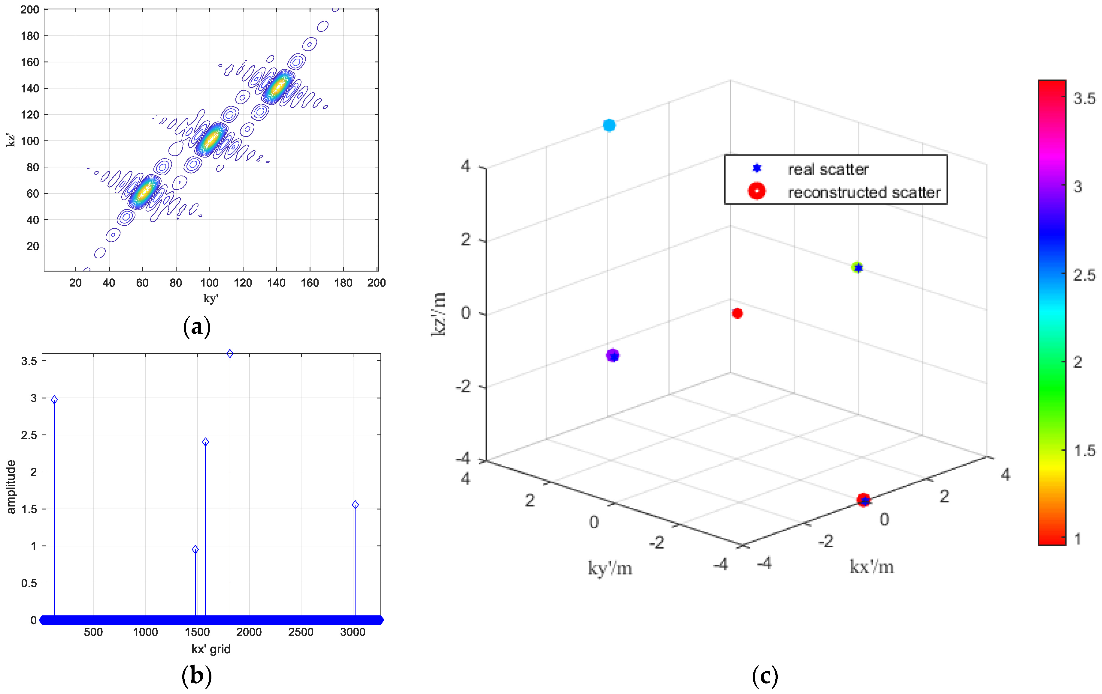
| True | 1.00 | 2.40 | 3.60 | 1.60 | 3.00 | (0, 0, 0) | (0, 4, 4) | (0, 4, −4) | (4, 0, 0) | (−4, 0, 0) |
| Reconstructed | 0.948 | 2.40 | 3.578 | 1.558 | 2.973 | (−0.02, 0, 0) | (0.10, 4, 4) | (−0.13, 4, −4) | (4.07, 0, 0) | (−4.05, 0, 0) |
| Parameters | Reflection Coefficients | 3D Positions | ||||||||||||
|---|---|---|---|---|---|---|---|---|---|---|---|---|---|---|
| True | 10.00 | 10.00 | 10.00 | 10.00 | 10.00 | 10.00 | 10.00 | (0, 0, 0) | (0, 4, 4) | (0, 4, −4) | (4, 0, 0) | (−4, 0, 0) | (0, 4, 0) | (0, −4, 0) |
| Reconstructed | 9.83 | 9.94 | 9.81 | 9.93 | 9.93 | 9.90 | 9.86 | (−0.02, 0, 0) | (0.10, 4, 4) | (−0.13, 4, −4) | (4.07, 0, 0) | (−4.05, 0, 0) | (0.05, 4, 0) | (−0.08, −4, 0) |
Disclaimer/Publisher’s Note: The statements, opinions and data contained in all publications are solely those of the individual author(s) and contributor(s) and not of MDPI and/or the editor(s). MDPI and/or the editor(s) disclaim responsibility for any injury to people or property resulting from any ideas, methods, instructions or products referred to in the content. |
© 2024 by the authors. Licensee MDPI, Basel, Switzerland. This article is an open access article distributed under the terms and conditions of the Creative Commons Attribution (CC BY) license (https://creativecommons.org/licenses/by/4.0/).
Share and Cite
Gu, T.; Guo, Y.; Zhao, C.; Zhang, J.; Zhang, T.; Liao, G. Thorough Understanding and 3D Super-Resolution Imaging for Forward-Looking Missile-Borne SAR via a Maneuvering Trajectory. Remote Sens. 2024, 16, 3378. https://doi.org/10.3390/rs16183378
Gu T, Guo Y, Zhao C, Zhang J, Zhang T, Liao G. Thorough Understanding and 3D Super-Resolution Imaging for Forward-Looking Missile-Borne SAR via a Maneuvering Trajectory. Remote Sensing. 2024; 16(18):3378. https://doi.org/10.3390/rs16183378
Chicago/Turabian StyleGu, Tong, Yifan Guo, Chen Zhao, Jian Zhang, Tao Zhang, and Guisheng Liao. 2024. "Thorough Understanding and 3D Super-Resolution Imaging for Forward-Looking Missile-Borne SAR via a Maneuvering Trajectory" Remote Sensing 16, no. 18: 3378. https://doi.org/10.3390/rs16183378