Article

Contrastive Transformer Network for Track Segment Association with Two-Stage Online Method

1
School of Electronic and Optical Engineering, Nanjing University of Science and Technology, Nanjing 210094, China
2
Xi’an Electronic Engineering Research Institute, Xi’an 710199, China
*
Author to whom correspondence should be addressed.
Remote Sens. 2024, 16(18), 3380; https://doi.org/10.3390/rs16183380
Submission received: 20 July 2024 / Revised: 29 August 2024 / Accepted: 8 September 2024 / Published: 11 September 2024
(This article belongs to the Topic Radar Signal and Data Processing with Applications)

Abstract

:
Interrupted and multi-source track segment association (TSA) are two key challenges in target trajectory research within radar data processing. Traditional methods often rely on simplistic assumptions about target motion and statistical techniques for track association, leading to problems such as unrealistic assumptions, susceptibility to noise, and suboptimal performance limits. This study proposes a unified framework to address the challenges of associating interrupted and multi-source track segments by measuring trajectory similarity. We present TSA-cTFER, a novel network utilizing contrastive learning and TransFormer Encoder to accurately assess trajectory similarity through learned Representations by computing distances between high-dimensional feature vectors. Additionally, we tackle dynamic association scenarios with a two-stage online algorithm designed to manage tracks that appear or disappear at any time. This algorithm categorizes track pairs into easy and hard groups, employing tailored association strategies to achieve precise and robust associations in dynamic environments. Experimental results on real-world datasets demonstrate that our proposed TSA-cTFER network with the two-stage online algorithm outperforms existing methods, achieving 94.59% accuracy in interrupted track segment association tasks and 94.83% in multi-source track segment association tasks.

1. Introduction

In the field of radar data processing, track interruption poses a frequent and significant challenge that hinders continuous target tracking. Factors such as target maneuvering, erroneous associations, and low detection probability contribute to this problem [1]. In addition, there is a growing research focus on the joint detection and tracking of targets using multiple sensor networks. To enable subsequent trajectory fusion processing, it becomes crucial to associate tracks obtained from different sensors, including radars or the automatic identification system (AIS), that correspond to the same target [2].
Traditional methods for interrupted track segment association (ITSA), as described in [3,4], rely on an a priori hypothesis model of target motion. These methods involve forward prediction or backward retrodiction between the end of the old track segment and the start of the new track segment, providing a framework for linking the track segments. If the predicted or retrodicted trajectory satisfies certain discriminative criteria, it is considered associated. In [5], a method was used that combined constant acceleration (CA) and coordinated turn (CT) models. The study explored various model parameters, such as accelerations and turn rates, to accurately model target motion characteristics. Fuzzy similarity measures were then applied to assess correlations between interrupted tracks. Similarly, in [1], researchers addressed interruptions in target tracking using a constant velocity (CV) model for continuous motion and switching to a CT model during interruptions within a two-dimensional (2-D) assignment framework. They optimized interruption associations by varying turn rates and employed a 2-D matching algorithm [6] to achieve a globally optimal solution. When the actual motion of the target does not match the a priori assumptions, it is difficult to guarantee the performance of the association.
Traditional multi-source track segment association (MSTSA) techniques aim to address system biases and random errors inherent in different sensors by employing various criteria such as statistics, structural similarity, fuzzy logic, etc. In [7], a novel track-to-track association algorithm was introduced, which uses the reference topology feature to mitigate sensor biases. Furthermore, the research outlined in [8] took a novel approach by transforming the association problem into a non-rigid point-matching problem and incorporated structural similarity to improve performance. In addition, in [9] an innovative algorithm is proposed that utilizes a dynamic weight function. By integrating target position information into the weight function and dynamically updating the fuzzy weight set, this improved algorithm achieved superior results in dense target scenarios. Inconsistent sensor noise levels can affect the performance of these methods. Moreover, thresholds often have to be determined manually, making it difficult to find a satisfactory global value.
Traditional techniques often suffer from inherent limitations, including unrealistic model assumptions, sensitivity to noise, reliance on manual thresholding, and suboptimal performance limits, etc. [1,10]. Nevertheless, in recent years, data-driven deep-learning methods have gained considerable attention in the domain of track segment association. These methods effectively learn feature representations of trajectories from the data, offering increased flexibility and accuracy.
For the ITSA problem, in [10], a combination of Long Short-Term Memory (LSTM) [11] and convolutional neural network (CNN) was utilized to capture temporal and spatial information from trajectories. This enables the comparison of feature similarity between trajectories to determine whether they belong to segments of the same target. Meanwhile, in [12], a graph neural network was employed to extract local track point embeddings at the node level and track graph embeddings at the graph level, facilitating the association of interrupted track segments. The authors above meticulously designed network architectures tailored to trajectory data and, in static environments, determined whether the trajectories belonged to the same target by comparing their similarity. However, neither considered the dynamic nature of real-world scenarios, where target trajectories can appear or disappear at any time. It is necessary to dynamically calculate similarity and make assessments based on changes in trajectories.
As for the MSTSA problem, the authors of [2] introduced using a spatial-temporal mixing extraction block to extract features from both tracks and scenes. These extracted features were then used to estimate the homography matrix, which helped to provide clear discriminants and improve the credibility of association decisions. In another study [13], the authors employed an autoencoder to efficiently denoise initial track data. They subsequently utilized a fully connected layer to extract high-dimensional features from the tracks, capturing the essential characteristics and patterns inherent in the data. Furthermore, a 3-D convolutional layer was incorporated to capture the features of the scene, providing valuable contextual information about the surrounding environment. Finally, the combination of features extracted from both tracks and scenes was used to assess the likelihood of two tracks originating from a common target. Similar to ITSA, the authors did not account for dynamic changes in the scene. Instead, they [2,13] used the complete temporal trajectory information to make associations between trajectories, rather than using all the information available up to the present moment.
In this paper, we address the problem of associating interrupted and multi-source track segments within a unified framework, which has not been previously discussed together in the literature [2,10,12,13]. Firstly, we transform the track segment association problem into a trajectory similarity measurement problem following [10,12]. By comparing the distances between high-dimensional features of trajectories, we can determine if they belong to the same target. Typically, trajectories from the same target exhibit high similarity. This approach contrasts with traditional methods that rely on motion model-based predictions for associating interrupted trajectories, thus avoiding performance degradation caused by mismatched motion models. Next, we introduce the TSA-cTFER network to extract high-dimensional feature representations of trajectories. For the input trajectory data, we initially convert the continuous and discrete attributes into vector representations using linear mapping and lookup tables. We then leverage the robust feature extraction capabilities of the Transformer Encoder. This is followed by pooling the information across the entire temporal dimension, as illustrated in Figure 1. This process provides comprehensive insights into the characteristics and behaviors of the trajectories. To train the network, we employ contrastive learning. In both the ITSA and MSTSA tasks, we consider track segments from the same target as positive samples and tracks from different targets as negative samples. This objective function allows us to continuously decrease the distance between positive samples while increasing the distance between negative samples, allowing the network to learn discriminative features effectively. Finally, considering the dynamic nature of real-world scenarios, we propose a two-stage online association algorithm that leverages the high-dimensional features obtained from TSA-cTFER. This algorithm efficiently handles trajectories that may appear or disappear at any time. In the first stage, we categorize potential association pairs into easy and hard pairs based on their similarity differences. Then, in the second stage, we implement delayed decisions to enhance the accuracy of challenging association pairs, significantly improving the overall performance of trajectory associations. Effectively addressing the TSA problem not only improves target tracking accuracy but also enables improved situational awareness and decision-making capabilities in various applications, including surveillance, navigation, and transportation.
In summary, the main contributions of this paper are as follows:
  • From the perspective of trajectory similarity measurement, we unify the problems of interrupted track segment association and multi-source track segment association under a unified framework.
  • To tackle these challenges, we introduce a network called TSA-cTFER, which combines contrastive learning with the Transformer Encoder to produce high-dimensional feature representations of trajectories. This network effectively transforms the task of trajectory similarity calculation into a distance measurement problem in a high-dimensional vector space.
  • Furthermore, in dynamic scenarios where targets may appear or disappear unpredictably, we present a two-stage online association algorithm. This algorithm adapts different association strategies based on the difficulty levels of association pairs, enhancing association accuracy and reducing error rates.
The organization of this paper is as follows: Section 2 unifies the problem of ITSA and MSTSA in a unified framework and builds a model for the problem to be solved. Section 3 introduces in detail the network architecture based on the Transformer Encoder, as well as the contrastive loss function, and focuses on the construction method of positive and negative association pairs. In Section 4, we propose a two-stage online association algorithm for the practical application scenario of track segment association. Finally, in Section 5, we verify the effectiveness of the proposed TSA-cTFER network with the two-stage online algorithm through comparative experiments carried out with real-world data.

2. Problem

As for the ITSA problem, when track segmentation occurs, a tracking algorithm may create two tracks. The first track is the old one, which is terminated because there is no new information associated with the tracking target. The second track is a young one, following the same target, which is initialized and confirmed after the break. Given two lists of tracks, a track segment association algorithm must find the correct match between old and new tracks to maintain a consistent track ID.
Suppose that at the current time k, there exists an old track segment list containing tracks that have been terminated and a young track segment list consisting of tracks that have been started recently. They can be expressed as follows [1,3]
T k O = { T n O ( k ) ; n = 1 , , N }
T k Y = { T m Y ( k ) ; m = 1 , , M }
where N and M are the total number of old and young track segments, respectively. T n O ( k ) and T m Y ( k ) are the state vector of the target of the old track segment and young track segment following
T n O ( k ) = { s ^ k n ; k = k n , s O , , k n , e O } , n = 1 , , N
T m Y ( k ) = { s ^ k m ; k = k m , s Y , , k m , e Y } , m = 1 , , M
In (3), k n , s O and k n , e O are the start and end times of the nth old track segment, respectively. Similarly, in (4), k m , s Y and k m , e Y are the start and end times of the mth young track segment, respectively. s ^ k · is the state vector of the target at time k containing the moving information. For instance, when considering the information obtained from radar, the target trajectory state s ^ k · can be expressed as [ p x k , p y k , v x k , v y k ] . Here, p x k and p y k denote the target’s position in a 2D Cartesian coordinate system, and v x k and v y k represent the target’s velocity.
As for the MSTSA problem, it is essential to accurately match the target trajectory information reported by different sensors for the same target. Suppose that at the current time k, there are two sources, denoted as A and B , present in the scenario. These sources may belong to the same category, such as both being radar devices, or they could be of different categories, like radar and AIS devices. It is worth noting that the multi-source track segment association problem can be broken down into pairwise association problems between any two sources. Therefore, here we only consider the association problem between two sources. Taking into account that the target trajectory information reported by source A and B are represented as
T k A = { T i A ( k ) ; i = 1 , , I }
T k B = { T j B ( k ) ; j = 1 , , J }
where I , J is the total number of track segments reported on behalf of source A and B , respectively. Similarly to T n O ( k ) and T m Y ( k ) in (3) and (4), T i A ( k ) and T j B ( k ) denote the state vector of the target of source A and B .
It can be seen from (1), (2), (5) and (6) that both the ITSA and MSTSA problems can determine whether two tracks belong to the same target by comparing the similarity of the tracks between two lists. Therefore, this paper considers these two problems together.
For each target’s state vector T · · ( k ) in (1), (2), (5) and (6), we feed it into a neural network f θ represented by the parameter θ . This network then maps the state vector to a high-dimensional vector z R D that encompasses almost all the information on the trajectory. In this way, the similarity between the two tracks can be determined by comparing the distances in high-dimensional vector spaces. If two tracks are associated with the same target, their distance is smaller than that of the others. Taking the ITSA problem as an example, the distance between two tracks is calculated as follows
z n O ( k ) = f θ ( T n O ( k ) ) z m Y ( k ) = f θ ( T m Y ( k ) ) d n , m ( k ) = sim ( z n O ( k ) , z m Y ( k ) )
where sim ( · , · ) : R D × R D R is a distance measure and more details about it is described in Section 3.5.
Once we obtain the distances between two tracks, we can construct the global distance matrix D k at time k.
D k = [ d n , m ( k ) ] N × M
Therefore, the optimal match can be obtained by maximizing the following expression [3]
max a n , m A k D k = n = 0 N m = 0 M a n , m d n , m
where A k is an assignment matrix, whose elements are binary, and
a n , m = 1 if tracks T n O ( k ) and T m Y ( k ) are from the same target 0 else .
Considering that each track can only be associated with another track or not associated with any track, Equation (9) satisfies the following constraint [3]
n = 0 N a n , m = 1 , m = 1 , , M m = 0 M a n , m = 1 , n = 1 , , N
where n = 0 and m = 0 indicate dummy tracks in the old track segment list T k O and young track segment list T k Y , respectively.
Observing that (9) describes a 2-D assignment problem, as the time k varies, Equation (9) evolves into a multi-dimensional (M-D) assignment problem, which is typically complex and time-consuming to resolve. Furthermore, existing methods [2,10,12,13] mainly focus on the static association issue without accounting for temporal changes as described in Section 1. Therefore, this paper first considers solving the 2-D assignment problem at time k, and then adopts a greedy algorithm to solve the temporal variation case, that is, designing a two-stage online matching strategy to achieve track association, thereby avoiding directly solving the M-D assignment. Further details will be provided in Section 4.

3. Proposed Method

In this section, we will begin by presenting the overall framework of TSA-cTFER. Subsequently, a detailed explanation will be provided for each component, including the input embedding module, the Transformer Encoder module, and the output pooling module. In addition, we will discuss the construction of positive and negative pairs and the contrastive loss functions utilized during training.

3.1. Overall Framework

The overall network framework, as depicted in Figure 2, comprises three modules: the input embedding module, the Transformer Encoder module, and the output pooling module. The input embedding module is tasked with processing various input data attributes and converting them into a unified vector representation. Subsequently, the Transformer Encoder module extracts features from the trajectories, which are then passed through the output pooling module to map the trajectories onto high-dimensional vectors. Here, we use two parallel pooling heads to obtain high-dimensional vector representations for the tasks of ITSA and MSTSA, respectively.

3.2. Input Embedding Module

The input embedding module maps different attributes of the targets to vectors of the same dimension, facilitating further processing by the network. Specifically, the attributes of the targets can be divided into continuous attributes and discrete attributes, as shown in Figure 2b.
Continuous attributes such as position, velocity, heading, etc., are first preprocessed through z-score standardization preprocessing and then linearly mapped to a D-dim vector. Suppose that x c R x L × D c are the preprocessed continuous attributes, where x L is the length of the trajectory and D c is the number of continuous attributes. A linear projector is then used to obtain a D-dim embedding vector, denoted as x ^ c , which can be computed as follows
x ^ c = x c W c R x L × D
where W c R D c × D are the network parameters that need to be learned.
For discrete attributes such as target type, detection timestamp, source ID, etc., we use one-hot encoding to represent them. In the one-hot encoding, each discrete attribute is represented by a fixed-length binary vector. The length of the binary vector is equal to the number of unique discrete attributes. Each element in the vector corresponds to a specific discrete attribute, and only one element is set to 1 while all the others are set to 0. Thus, discrete attributes can be mapped to a D-dim vector through a lookup table following
x ^ d = x d W d R x L × D
where x d [ 0 , 1 ] x L × D d is the one-hot binary vector, D d is the number of unique discrete attributes, and W d R D d × D are the network parameters that need to be learned.
After obtaining the continuous and discrete embeddings of a trajectory, we add them at the corresponding time steps and then pad them with a learned padding token  E p a d R D to meet the specified length requirement of the network. Following that, a non-linear transformation is applied along with positional encoding [14] to obtain the final input embedding representation as follows
x ^ = NonLinear ( cat [ x ^ c + x ^ d ; E p a d , , E p a d ] ) R N × D z 0 = x ^ + P p o s R N × D
where cat [ · , · ] represents the concatenation operation. The non-linear transformation consists of a ReLU activation function [15] and a linear projection. The positional encoding P p o s R N × D contains information about the point position in the trajectory [14], which is shown as follows
P p o s , 2 i = sin ( p o s / 10,000 2 i / D ) P p o s , 2 i + 1 = cos ( p o s / 10,000 2 i / D )
where p o s is the point position in the trajectory and i is the dimension.

3.3. Transformer Encoder Module

As shown in Figure 2c, the Transformer encoder structure consists of L layers of identical Transformer Encoder blocks. Each Transformer Encoder block includes a multi-head self-attention (MSA) module and a Feed-Forward Network (FFN) module. Incorporation of residual connections [16] and layer normalization [17] within each block facilitates efficient propagation of information and promotes stable training.

3.3.1. Multi-Head Self-Attention

The multi-head self-attention mechanism in the Transformer Encoder block is a crucial component that allows it to capture dependencies and relationships within an input sequence effectively. Initially, the input embeddings z l R N × D are transformed into multiple sets of query q , key k , and value v matrices through linear transformations [14,18].
[ q , k , v ] = z l W q k v , W q k v R D × 3 D h
where D h is the dimension of each attention head. To maintain a constant computational load and keep the number of parameters consistent when adjusting the number of heads h, D h is usually set to D / h .
Next, the self-attention weights A are computed by taking the scale dot product between q and k , followed by applying a masked softmax function.
A = softmax ( M A · ( q k T / D h ) ) R N × N
where M A [ 0 , 1 ] N × N is a masked matrix, all padding tokens will be masked and excluded from the self-attention weights A computation.
Finally, the weighted sum of the value matrices v is calculated using the self-attention weights A .
SA ( z l ) = A v R N × D h
Instead of performing a single self-attention operation, the aforementioned process is repeated h times to obtain a multi-head self-attention. Each head in the multi-head self-attention has its own set of weight matrices for query, key, and value calculations. The outputs of all heads are subsequently concatenated into a matrix, which is further projected to yield the final representation.
MSA ( z l ) = cat [ SA 1 ( z l ) ; ; SA h ( z l ) ] W m s a R N × D

3.3.2. Feed-Forward Network

The position-wise fully connected feed-forward network employs a non-linear transformation to enhance the expressive capabilities of the network [14,18]. This transformation is applied independently and uniformly to each position. It comprises two linear transformations with a GELU activation function [19] in between.
FFN ( z ) = GELU ( z W f 1 + b f 1 ) W f 2 + b f 2
where W f 1 R D × D f f , b f 1 R D f f , W f 2 R D f f × D and b f 2 R D are all learnable parameters.

3.3.3. Block Connecting and Layer Stacking

In each layer of the Transformer Encoder block, a combination of residual connection and layer normalization is utilized to connect the multi-head self-attention block with the feed-forward network block. The output of the previous layer acts as the input of the next layer. By stacking L layers together, the Transformer Encoder structure is constructed [14,18].
z l = MSA ( LN ( z l 1 ) ) + z l 1 ,   l = 1 , , L
z l = FFN ( LN ( z l ) ) + z l , l = 1 , , L
where z 0 is obtained from (14) and a layernorm operation [17] is applied before every block. Layer normalization standardizes each feature dimension to have zero mean and unit variance. This effectively addresses the issues of vanishing and exploding gradients, enhancing the stability and convergence speed of the network.

3.4. Output Pooling Module

The Transformer Encoder module produces an output matrix z L of size N × D . To obtain a fixed-length trajectory representation with a dimension of D, a pooling module is applied to process the context matrix z L . As shown in Figure 2a, we obtain trajectory feature representations for the ITSA task and the MSTSA task separately using two parallel projection heads after the same pooling operation. Initially, z L goes through a pooling layer and then outputs trajectory features through a linear mapping.
z ^ L = pooling ( z L ) R D z o u t ITSA = z ^ L W ITSA R D z o u t MSTSA = z ^ L W WSTSA R D
where W ITSA , W WSTSA R D × D are the learnable projection heads for ITSA and MSTSA task, respectively.
We experiment with three pooling strategies:
CLS-strategy
Like class-token described in previous works such as ViT [18] and BERT [20], we introduce a trainable embedding x c l s at the beginning of the embedded sequence. The state of this embedding at the output of the Transformer Encoder serves as a representation of the entire trajectory.
x ^ 0 = NonLinear ( cat [ x c l s ; x ^ c + x ^ d ; E p a d , , E p a d ] ) z 0 = x ^ 0 + P p o s z ^ L = LN ( z ^ L 0 ) R D
Here, z ^ L 0 corresponds to the input class-token x c l s and is located at the beginning of the output state.
MEAN-strategy
MEAN-strategy computes the mean-over-time of the context matrix z L . It calculates the average value of each column in z L and returns a D-dim vector z ^ L .
z ^ L = mean ( M z · z L , axis = 0 ) R D
Here, axis = 0 indicates that the mean operation is performed on each column of the matrix z L and M z [ 0 , 1 ] N × D is a masked matrix similar to M A , where the D column vectors are identical, and the first x L elements in each of the N rows are active.
MAX-strategy
Similar to the MEAN-strategy, MAX-strategy computes the max-over-time of the context matrix z L as follows
z ^ L = max ( M z · z L , axis = 0 ) R D
Thus, we obtain high-dimensional feature representations for each trajectory.

3.5. Contrastive Loss Function

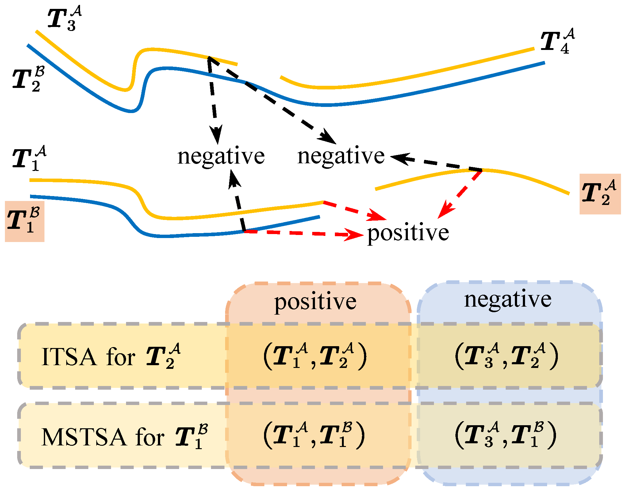
We use the contrastive loss [21,22] as an objective function. Contrastive learning is a technique that aims to enhance the learning of data representations by creating pairs of positive and negative samples, and continuously minimizing the dissimilarity between similar data instances while maximizing the dissimilarity between dissimilar ones. In the context of ITSA, positive samples are defined as track segments that belong to the same target before and after an interruption, whereas negative samples represent track segments between different targets. For the MSTSA problem, positive samples refer to track segments from different sources that correspond to the same target. In contrast, negative samples indicate track segments between different sources and distinct targets.
As illustrated in Figure 3, let us assume that there are two sources, denoted A and B , that continuously provide trajectory information for two distinct targets. The track segments of the same target may be interrupted for various reasons; for instance, T 1 A and T 2 A represent such interrupted track segments. Additionally, track segments of the same target detected by different sources may exhibit positional discrepancies due to source system errors, as seen with T 1 A and T 1 B representing multi-source track segments. Therefore, it is crucial to determine which track segments belong to the same target. In this context, Track T 1 A , T 1 B and T 2 A belong to the track segment of the same target, and Track T 3 A , T 2 B and T 4 A belong to the segment of another distinct target. For the ITSA task, consider T 2 A as an example, assuming the current old track set is { T 1 A , T 3 A , T 1 B } , since ITSA only matches tracks from the same source, so T 1 B will not match with T 2 A . Consequently, ( T 1 A , T 2 A ) are positive pairs and ( T 3 A , T 2 A ) are negative pairs based on whether the track segments are from the same target. For the MSTSA task, take T 1 B as an example. If the current set of existing tracks is { T 1 A , T 3 A , T 2 B } , MSTSA only matches tracks generated by different sources, so T 2 B will not match with T 1 B . Then, ( T 1 A , T 1 B ) are positive pairs and ( T 3 A , T 1 B ) are considered negative pairs based on whether the track segments are from the same target.
Given a collection of paired track samples D = { ( T m , T m + ) } m = 1 M , where T m and T m + represent positive track samples from the same target. During training, we randomly select B track pairs from D to create a mini-batch of 2 B sample points. Thus, for each track sample T i , there is a similar sample T j in the mini-batch, with the remaining 2 ( B 1 ) samples considered negatives. Following the approach in [21,22], InfoNCE is used as the loss function. The loss function for a given positive sample pair ( T i , T j ) is defined as
i , j = log exp ( sim ( z i , z j ) / τ ) k = 1 2 B 1 k i exp ( sim ( z i , z k ) / τ )
where B is the mini-batch size, z i , z j , z k are obtained from (7), 1 [ k i ] { 0 , 1 } is an indicator function that evaluates to 1 iff k i and τ denotes a temperature hyperparameter. As described in (7), we adopt cosine similarity as a distance measure here, defined as
sim ( u , v ) = u T v / ( u v )
where · denotes 2 norm. Therefore, the total loss t o t a l is defined as
t o t a l = 1 2 B i = 1 2 B j = 1 2 B i , j ( i , j ) positive pairs
In the InfoNCE loss function (27), the numerator term represents the similarity of the positive samples, while the denominator term sums the similarities among all samples except for itself. The temperature parameter τ controls the smoothness or sharpness of the similarity distribution. A higher τ leads to smaller differences in similarity values between positive and negative samples, while a lower τ increases these differences. The choice of the temperature parameter τ is usually based on experimental results as shown in Section 5.6.

4. Two-Stage Online Association Algorithm

The online TSA algorithm divides the entire association process into two parts. The first part is the track state update module, which uses the continuously received target information from the sensors to update the target state. The second part is the proposed two-stage association algorithm. In association scenarios, there are both simple track pairs that can be easily associated and difficult track pairs that pose challenges for the association. To address these varying complexities, we employ different association strategies to handle them accordingly. The comprehensive tracking process is illustrated in Figure 4 and will be expounded on in the subsequent sections.

4.1. Track State Update

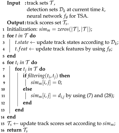
The trajectory information of the target is continuously sent by the sensors. The track state update module is responsible for recording the states of the targets, which includes sensor ID, timestamp, position, velocity, and other relevant information. Currently, it utilizes the neural network f θ for TSA to constantly update the representation of the trajectory. A detailed description of the entire track state update process is provided in Algorithm 1.
Lines 2 to 5 of Algorithm 1 update the state and feature representation of the trajectories using the sensor detection results D k at the current time step k. The similarity between the two trajectories is then computed using the Equations (7) and (28). The function filtering ( t i , t j ) on line 8 of Algorithm 1 filters out certain pairs of trajectories that do not meet the association criteria. This filtering is performed by taking into account information such as timestamp, position, and velocity. In the case of ITSA, it is necessary to consider that there is a temporal sequential relationship between the trajectories for which similarity must be computed, while trajectories that appear simultaneously do not require similarity computation. In the context of the MSTSA problem, trajectories belonging to the same target are usually close to each other. By comparing the positional differences between the two trajectories at the same time, the distant trajectories can be filtered out to reduce the computational load in subsequent steps.
It is essential to emphasize that the length of the input data for the feature extractor f θ on line 4 of Algorithm 1 may vary depending on the specific requirements of f θ . For instance, in TSA-cTFER with a fixed input size N, if a trajectory is longer than the specified length, it may need to be truncated by retaining only the most recent data points to meet the length requirement.
Algorithm 1: Track State Update.
Remotesensing 16 03380 i001

4.2. Two-Stage Association Method

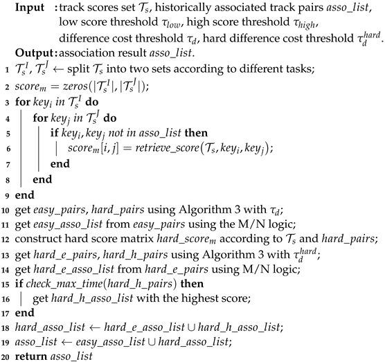
As previously mentioned, the two-stage association approach classifies candidate track pairs into easy and hard pairs based on the disparity in their similarity. The entire process of the two-stage association method is described in Algorithm 2.
First, the set of track scores T s is divided into two distinct sets, denoted as T s I and T s J according to the specific task at hand, as described in line 1 of Algorithm 2. For the ITSA problem, T s is categorized into old track sets T s O and young track sets T s Y based on timestamp information to determine whether the track has ended. For the MSTSA problem, considering the different source IDs and timestamps, tracks from the same source sensor at the current moment are grouped, resulting in T s A and T s B .
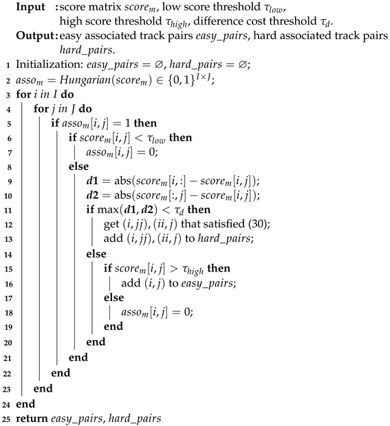
Subsequently, a score matrix s c o r e m is constructed based on the similarities obtained from Algorithm 1. The Hungarian algorithm [6] is then employed to solve the matrix, yielding candidate association pairs. It is important to note that the introduction of dummy tracks in (11) is primarily intended to indicate that certain tracks may not have corresponding associated tracks. In this context, dummy tracks are not explicitly constructed; instead, the matching results of the Hungarian algorithm are re-evaluated, and some track associations with low similarities are discarded. Candidate association pairs with a score value below τ l o w are directly labeled as invalid. Among the remaining candidate association pairs, those that have another pair with a score difference less than τ d are categorized as hard pairs; otherwise, if the association score is greater than τ h i g h , it is considered an easy pair, while the remaining pairs are considered invalid. The selection procedure for invalid/easy/hard association pairs is detailed in Algorithm 3 and illustrated in Figure 5. We primarily determine the existence of similar association pairs based on score differences, and then judge whether the association pair is considered an easy or hard case.
abs ( s c o r e m [ i , j j ] s c o r e m [ i , j ] ) < τ d for j j = 0 , 1 , , J 1 abs ( s c o r e m [ i i , j ] s c o r e m [ i , j ] ) < τ d for i i = 0 , 1 , , I 1
Algorithm 2: Two-Stage Association.
Remotesensing 16 03380 i002
Next, we employ a straightforward M/N logic to determine the successful association of pairs within the set e a s y _ p a i r s , as described in line 11 of Algorithm 2. This logic operates on the assumption that, out of M consecutive evaluations, if there are N instances of a particular association pair appearing in the set e a s y _ p a i r s , it is considered a valid association.
For all hard association pairs h a r d _ p a i r s , the hard score matrix h a r d _ s c o r e m is first reconstructed based on the set of track scores T s . Subsequently, Algorithm 3 is used to further classify the pairs into easy association pairs h a r d _ e _ p a i r s and hard association pairs h a r d _ h _ p a i r s using a difference cost threshold τ d h a r d ( < τ d ) . Then, the M/N logic is applied to easy association pairs h a r d _ e _ p a i r s to determine their association relationship. Conversely, the hard association pairs h a r d _ h _ p a i r s are retained for additional evaluation in the subsequent time step k + 1 until the maximum matching time requirement is met. At that point, the association pair with the highest score is directly selected as the output.
In summary, the selection of easy and hard association pairs, outlined in Algorithms 2 and 3, is based on the similarity of characteristics derived from the TSA network f θ . In scenarios involving multiple trajectories with high similarities, we adopt a deferred decision strategy that involves reevaluating associations upon receiving additional target trajectory information. Although this strategy may lead to increased association latency, it contributes to improved accuracy levels.
Algorithm 3: Select Easy/Hard Association Pairs.
Remotesensing 16 03380 i003

5. Experimental Results

5.1. Datasets

To assess the effectiveness of our approach, we utilized the Multi-source Track Association Dataset (MTAD) proposed in [23,24] as a standardized benchmark for evaluation purposes. The MTAD is constructed by performing various processing steps, such as grid partitioning, automatic interruption, and noise injection, on AIS trajectory data. This dataset contains millions of individual tracks, however, for our analysis, we are focusing solely on data from 5000 unique scenes. For each scene, trajectory information is reported from two sensors at different reporting rates: 10 s and 20 s. The entire scenario lasts approximately two hours. Each trajectory in the dataset is comprised of four-dimensional information, namely longitude, latitude, speed, and heading, describing the motion of the targets. As a result, each scene in this dataset contains varying numbers of tracks, ranging from several to hundreds. These tracks exhibit diverse movement patterns, target types, and duration periods. Hence, the MTAD is highly suitable for validating the performance of different track segment association algorithms.
As shown in Figure 6, the MTAD presents four typical association scenarios, which involve ITSA and MSTSA tasks. These scenarios exhibit varying characteristics. Some have a limited number of tracks with straightforward target motion, while others have a larger number of tracks that tend to concentrate on specific areas. Consequently, associating these tracks becomes more challenging.

5.2. Metrics

The two tracks that satisfy the following conditions are referred to as the actual associated track pairs AP [23]:
  • The tracks originate from the same target.
  • In the case of ITSA, the time interval between interruptions in the two tracks is required to be less than 20 min, and each track must have a duration longer than 2 min.
  • For the MSTSA problem, the intersection time of the two-track segments needs to exceed 2 min.
Thus, we define the set composed of all APs in a scene s as T AP s and the set composed of the associated pairs produced by the association algorithm as O AP s .
To measure the association accuracy, we define the association accuracy P C A s as [23]:
P CA s = | O AP s T AP s | | T AP s | × 100 %
where | · | indicates the number of association pairs in the set and ∩ is representing the intersection operation between sets.
Similarly, we can also obtain the definitions of association fault rate P FA s [23]:
P FA s = | O AP s O AP s T AP s | | O AP s | × 100 %
and the association latency T AP s [23]:
T AP s = 1 | O AP s T AP s | A P O AP s T AP s t AP s
where the latency t AP s is defined as the generation time of the association relationship between track pairs minus the association start time of that track pair. For ITSA, the association start time is defined as the time when the first point of the young track appears. For the MSTSA problem, the association start time is defined as the time when the first point of the later track appears.
Therefore, for all scenarios, the average association accuracy m P CA and the average weighted association accuracy m w P CA are, respectively, defined as [23]:
m P CA = 1 S s = 0 S 1 P CA s
m w P CA = s = 0 S 1 | O AP s | O AP P CA s
Here, S represents the total number of test scenarios and O AP = s = 0 S 1 | O AP s | . Similarly, we can obtain the definitions of average association fault rate m P FA , average weighted association fault rate m w P FA , average association latency m T AP s , and average weighted association latency m w T AP s .

5.3. Baselines

5.3.1. Traditional Methods

For the ITSA problem, traditional methods commonly depend on the prediction of the trajectories of targets and subsequently assessing the degree of similarity between two trajectories. If the predefined matching criteria are met, the corresponding pairs are deemed successful matches.
Multiple Hypothesis TSA: The Multiple Hypothesis TSA algorithm (MH TSA) [5] starts by constructing multiple potential models of target motion and performing trajectory prediction. Next, based on position and velocity information, a fuzzy correlation function is utilized to depict the relationship between predicted old tracks and new tracks. Finally, the Multiple Hypothesis TSA algorithm constructs a fuzzy similarity matrix between the old and young tracks and then employs the two-dimensional assignment principle to determine the association between targets.
Multi-Frame 2-D TSA: The Multi-Frame 2-D TSA algorithm (MF 2-D TSA) [1] assumes that the target motion follows the constant velocity model before and after interruption. Additionally, it incorporates a constant turn with a turning rate of w throughout the breakage period. By exploring various turning rates, if the distance between the predicted state of the old track and the state of the young track meets specific criteria, this correlation is deemed successful.
In the case of the MSTSA problem, it is common to employ distance-based measurements to quantify the similarity between two tracks.
Distance-Based TSA: The Euclidean distance (ED) is the most commonly used distance metric for track correlation as used in [23]. However, it assumes that trajectories are the same length. Here, we also utilize Dynamic Time Warping (DTW) [25,26,27] as a criterion to measure the similarity of multi-source tracks. Similar to ED, DTW is also a measure designed for time series and can be applied to trajectory data. However, unlike ED, DTW can align a point of one trajectory with one or more consecutive points of another trajectory. This flexibility makes DTW suitable for cases where track lengths vary or where there are temporal variations in the data.

5.3.2. Deep Learning Based Methods

TSADCNN: TSADCNN [10] uses a temporal and spatial information extraction module to extract track information. The temporal module, composed of LSTM, is responsible for capturing temporal information, while the spatial module, consisting of multi-scale CNN, extracts spatial information. Initially, the track information undergoes processing through the LSTM module to capture temporal dependencies. Then, it is fed to the CNN module to extract spatial features. By mapping the track data onto a high-dimensional space, TSADCNN determines whether the trajectories belong to the same target based on the similarity of high-dimensional vectors.
TGRA: Similar to TSADCNN, TGRA [12] utilizes a graph network to extract track information. It employs the Graph Isomorphism Network (GIN) [28] and Graph Convolutional Network (GCN) [29] to obtain node-level local representations of track points. Subsequently, the Graph Attention Network (GAT) [30] is employed to acquire representations at the graph level. In this way, This approach enables the extraction of high-dimensional representations that encompass both the spatial and temporal information of the entire trajectory.

5.4. Implementation Details

5.4.1. Data Preparation

The 5000 scenes in MTAD are split into three subsets: a training set, a validation set, and a test set, following an 8:1:1 ratio. During training, trajectory data from 4000 scenes is mixed into one dataset. For each training iteration, a batch of trajectories is randomly chosen from this dataset. Positive and negative samples are created using this batch for the network to learn from, as explained in Section 3.5. In the testing phase, data from each scene are evaluated independently. Simulated data sources provide target trajectory information every 20 s in chronological order. Using the two-stage online association algorithm detailed in Section 4 and involving various networks such as TSADCNN [10], TGRA [12], and our TSA-cTFER to compute trajectory similarity, the final association results are derived for each scene. These outcomes are compared with the ground truth associations to determine the final performance metrics. For deep learning-based TSA methods, the continuous attributes input into the network include longitude and latitude, while the discrete attribute is the timestamp.

5.4.2. Model Settings

In the TSA-cTFER model, we define the maximum input trajectory length as N = 128 , the hidden layer size as D = 64 , the number of model layers as L = 4 , and utilize an attention mechanism with h = 4 heads. Furthermore, the size of the hidden layer of the FFN is set as D f f = 4 D . For the TSADCNN model, we use the same input embedding module as in the TSA-cTFER model. The features then undergo processing through LSTM and multi-scale CNN layers, followed by the utilization of two parallel fully connected layers to extract features for ITSA and MSTSA tasks, respectively. It is worth mentioning that we do not require the temporal correlation matrix to be a square matrix, hence the symmetric constraint loss discussed in [10] is not applied in this model. In this setup, all feature dimensions are set to 64, a single-layer unidirectional LSTM network is employed, and within the multi-scale convolutional network, each scale’s feature dimension is halved while the channel count is doubled. Similarly, in the TGRA model, we make use of the same input embedding module and incorporate two parallel Track Graph Embedding modules to derive ITSA and MSTSA features, respectively. In this model, the final output feature dimension is 64, while the remaining parameters align with those outlined in [12].

5.4.3. Training Details

During the training phase, we employed random cropping as a data augmentation strategy to improve the model’s generalization ability. Specifically, for two track segments to be associated in the ITSA task, we randomly discarded the tail information of the young track since ITSA primarily focuses on the changes before and after interruptions; for positive track pairs in the MSTSA task, we randomly cropped the trajectory information at the same timestamps for the two tracks.
To compare the feature extraction capabilities of different deep learning models, all of these models were equipped with identical parameters (N/M = 3/6, τ l o w = 0.5 , τ h i g h = 0.7 , τ d = 0.1 , τ d h a r d = 0.05 ) in the context of the two-stage online association algorithm. This consistent configuration allows for a comprehensive evaluation and comparison of the ability of the models to extract meaningful features.
During the training period, we trained all data for 150 epochs with a batch size of 512. We use Adam optimizer [31] with β 1 = 0.9 , β 2 = 0.999 , and ϵ = 10 6 . After 10 epochs of warmup, the learning rate decreased following a half-cycle cosine [32]. Additionally, a Dropout technique [33] with a dropout probability of 0.1 was applied as a regularization method during the training of TSA-cTFER. All experiments are carried out on a 64-bit workstation with the PyTorch deep learning framework [34]. The detailed configurations for these experiments are as follows: Ubuntu 22.04.3 LTS, 64 GB RAM, Intel Xeon E5-2690 CPU @ 2.60 GHz, NVIDIA GeForce RTX 3090 GPU.

5.5. Performance Analysis

For deep learning-based TSA methods, we independently trained each network three times and reported the average and standard deviation of the final results. In addition, we separately trained and co-train the ITSA and MSTSA tasks to observe the strength of the network’s ability to represent trajectories.

5.5.1. ITSA Task

The results of the ITSA task using different methods are displayed in Table 1, where “Sep.” indicates that only interrupted track data are utilized for training, and “#params.” represents the number of learnable parameters of the network. Among traditional interrupted TSA methods, Multiple Hypothesis TSA outperforms ED-based TSA and Multi-Frame 2-D TSA by a significant margin. Regarding deep learning-based methods, the results indicate that TSADCNN performs better when trained jointly rather than separately. Conversely, TGRA shows better performance with separate training for the two tasks. The separate and joint training results of TSA-cTFER are comparable, suggesting that TSA-cTFER possesses stronger representation capabilities than TSADCNN and TGRA. Furthermore, the association results of TSA-cTFER significantly outperform TSADCNN and TGRA, regardless of whether they were trained separately or jointly. Compared to the best results achieved by TSADCNN and TGRA, there is an increase of 11 % and 9 % in m P CA , respectively, alongside lower false association rates and faster association times. These findings underscore the superior ability of TSA-cTFER to extract trajectory characteristics.
It should be noted that the results of TSA-cTFER and Multiple Hypothesis TSA are similar, with TSA-cTFER demonstrating slightly superior association accuracy and lower error rates. However, it necessitates a longer average association time. This may be due to the significant correspondence between the motion model assumed by the Multiple Hypothesis TSA approach and the actual motion model in MTAD, contributing to its robust performance.

5.5.2. MSTSA Task

The results of the multi-source track segment association using different models are shown in Table 2. Traditional multi-source association methods based on distance metrics perform poorly in this task. In deep learning-based association methods, unlike the findings in the ITSA task, the performance of TSADCNN and TGRA improves significantly when trained separately for the MSTSA task compared to joint training for both tasks, resulting in an increase of approximately 1.8 % and 2.2 % in m P CA . However, TSA-cTFER shows consistent and better performance with fewer parameters, regardless of whether it is trained separately or jointly, highlighting its superior capability to represent trajectories compared to TSADCNN and TGRA. Furthermore, the performance gap between these three networks is minimal when trained separately, possibly because the MSTSA task is less complex than the ITSA task, as the trajectories of the MSTSA task exhibit greater similarity of spatial movement.

5.5.3. Analysis of a Typical Scenario

As shown in Figure 7a, a track segment association scenario in the MTAD is depicted. The scene depicts trajectory data recorded by two sensors, A and B , spanning a period of time, denoted as { A _ 0 , A _ 1 , A _ 2 , A _ 6 } and { B _ 0 , B _ 3 , B _ 5 } . Each trajectory maintains varying durations, originating from distinct starting points and concluding at different endpoints while displaying similar motion patterns.
As shown in Figure 7b, it illustrates the variation of association scores output by TSA-cTFER over time in the context of the ITSA task. For the track segment B _ 3 , there are two additional track segments, B _ 0 and B _ 5 , waiting to be associated. Here, B _ 0 represents the true track segment, while B _ 5 denotes the false one. Furthermore, it can be seen from Figure 7a that the direction of movement of B _ 5 is opposite to that of B _ 3 . By leveraging the robust trajectory representation capability of TSA-cTFER, the graph depicted in Figure 7b demonstrates a consistent decline in the association score of ( B _ 5 , B _ 3 ) below the threshold τ l o w , leading to its classification as an invalid pair and subsequent disregard by the association algorithm as described in Algorithm 3. On the contrary, the association score of ( B _ 0 , B _ 3 ) exceeds the threshold τ h i g h , indicating that it will be considered a correct association by Algorithm 3.
As shown in Figure 7c, it depicts the change in association scores output by TSA-cTFER in the MSTSA task. For track segment B _ 3 , there are four track segments A _ 0 , A _ 1 , A _ 2 , and A _ 6 that could be associated with it, with A _ 1 and A _ 2 being the true track segments. The substantial spatial overlap among these segments presents challenges for the association. In the initial association stage, B _ 3 may be associated with A _ 0 , A _ 1 , and A _ 6 . As more information is collected, the association score of the ( A _ 6 , B _ 3 ) output by TSA-cTFER decreases, indicating that A _ 6 and B _ 3 are becoming less similar. Meanwhile, both ( A _ 0 , B _ 3 ) and ( A _ 1 , B _ 3 ) show high similarity, but the similarity between A _ 1 and B _ 3 is higher. Combining this with the M/N logic in Algorithm 2, the association algorithm will consider ( A _ 1 , B _ 3 ) as the correct match. In the subsequent association stage, since A _ 0 was not associated with B _ 3 earlier, it will be excluded, leading to the association between A _ 2 and B _ 3 .
The variation in association scores in Figure 7 not only validates the powerful trajectory representation capability of TSA-cTFER, which combines contrastive learning to quickly and accurately assess trajectory similarity, but also demonstrates the effectiveness of the two-stage online association algorithm. This algorithm can address challenging association pairs by employing delayed matching and using more information to assist in the decision-making process.

5.6. Ablation Study

We performed ablation experiments on different components of TSA-cTFER to evaluate their specific impacts on the MTAD validation dataset. The ITSA and MSTSA tasks were concurrently trained for 100 epochs using the complete training dataset while ensuring that all other parameters remained consistent with those outlined in Section 5.4.3.
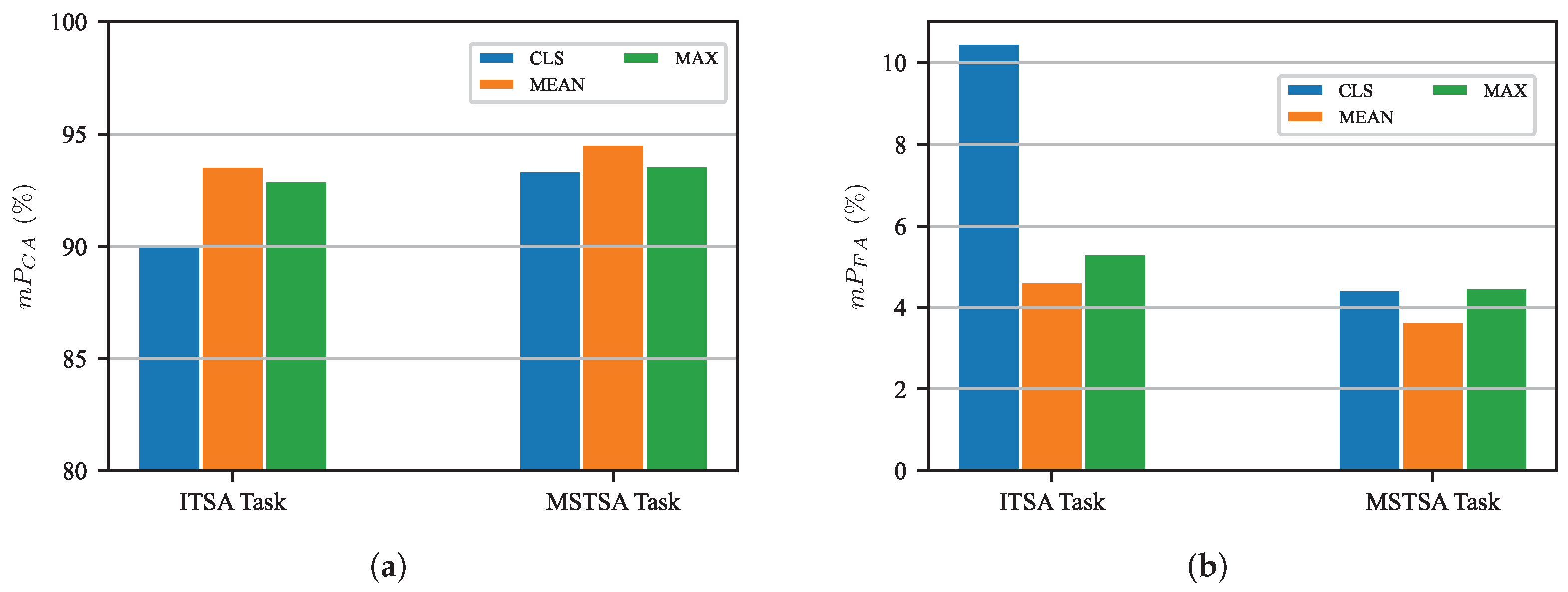
Effect of pooling strategy. We conducted tests, as described in Section 3.4, to investigate the influence of different pooling strategies on the results. As shown in Figure 8, regardless of the ITSA or MSTSA task, the MEAN-strategy outperforms others in both the metrics m P CA and m P FA . In comparison, the MAX-strategy performs slightly worse than the MEAN-strategy. Surprisingly, the commonly used CLS-strategy in [18,35] shows the worst performance in this experiment. This discrepancy might arise from the fact that the CLS-strategy relies solely on a single temporal feature output, while the MEAN-strategy and MAX-strategy leverage all temporal feature outputs, thus allowing them to capture long-term trajectory features more effectively.
Effect of input trajectory length. Different input trajectory lengths provide different amounts of information, with longer trajectories providing more insight into whether two trajectories originate from the same target. However, longer trajectories also introduce computational overhead and redundancy. Consequently, we experimented to determine the optimal input trajectory length. In Figure 9, it is observed that both ITSA and MSTSA show an improved average accuracy as the input trajectory length increases from 64 to 128, and MSTSA shows an increase of approximately 1.5 % . However, as the input trajectory length continues to increase from 128 to 256, the average accuracy of ITSA decreases. It is suggested that input trajectory lengths beyond a certain point do not provide additional useful information to improve the learning capabilities of the model.
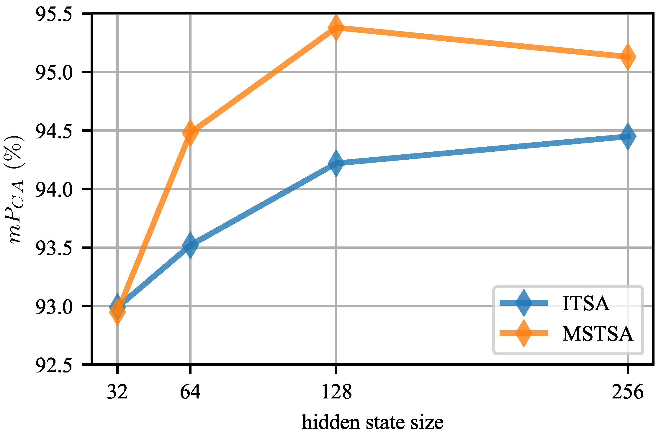
Effect of hidden state size. The sizes of hidden layers in a model determine its representation abilities. In Figure 10, when the hidden layer size is increased gradually from 32 to 256, there is an observed improvement in average accuracy for both ITSA and MSTSA tasks. The maximum improvement recorded is approximately 2 % . Therefore, it can be concluded that larger models tend to achieve higher average accuracy. However, it is important to note that larger models also require more GPU memory and training time during the training process.
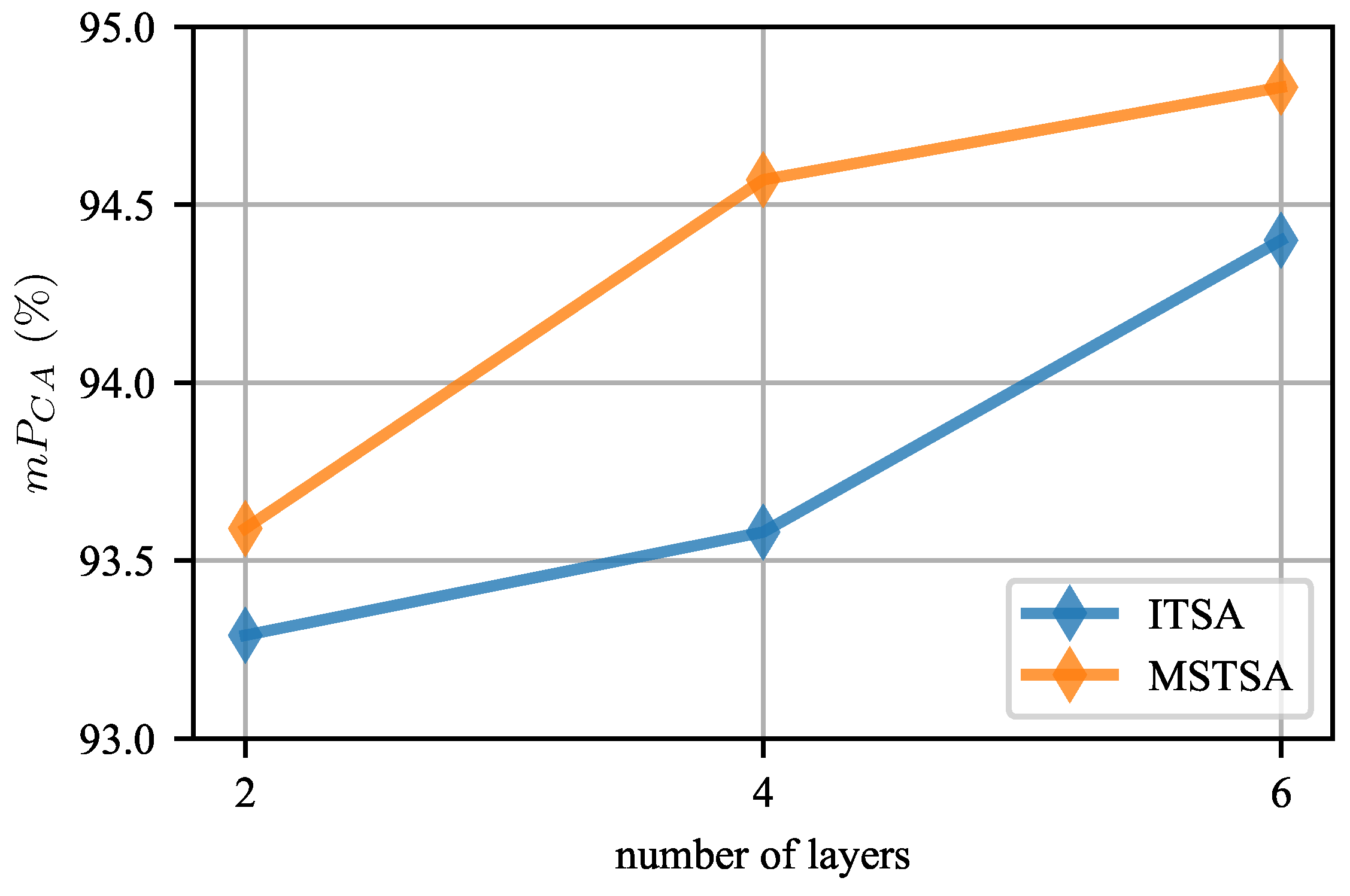
Effect of the number of layers. The depth of a model also affects its representational capacity. The deeper the model, the stronger its representational capacity. As shown in Figure 11, increasing the number of layers in the model from 2 to 6 resulted in an average accuracy improvement of approximately 1.3 % .
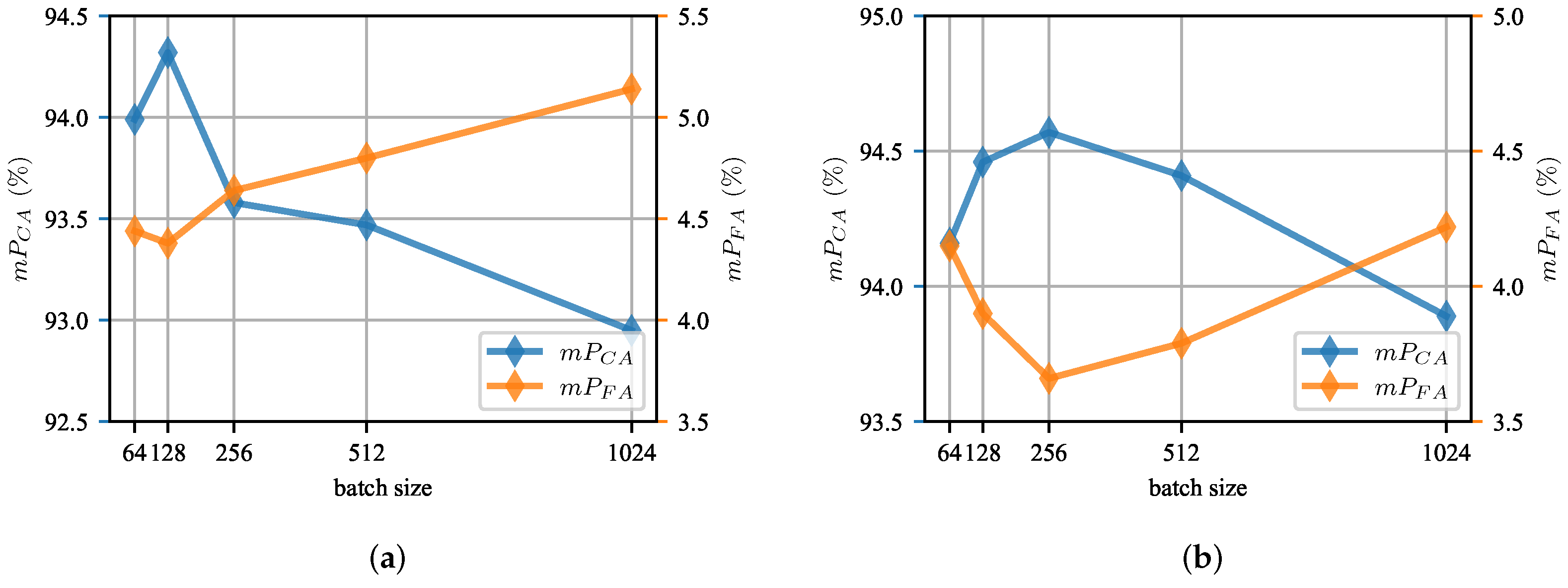
Effect of training batch size. The TSA-cTFER training utilizes a contrastive learning framework, which leverages data within the same batch to generate positive and negative samples. Generally, larger batch sizes provide more negative samples, enabling the model to achieve the specified accuracy quicker in fewer epochs. However, excessively large batch sizes can pose challenges during model training. As illustrated in Figure 12, both too small and too large batch sizes have an impact on network learning, but overall the influence of batch size on performance remains within 1 % .
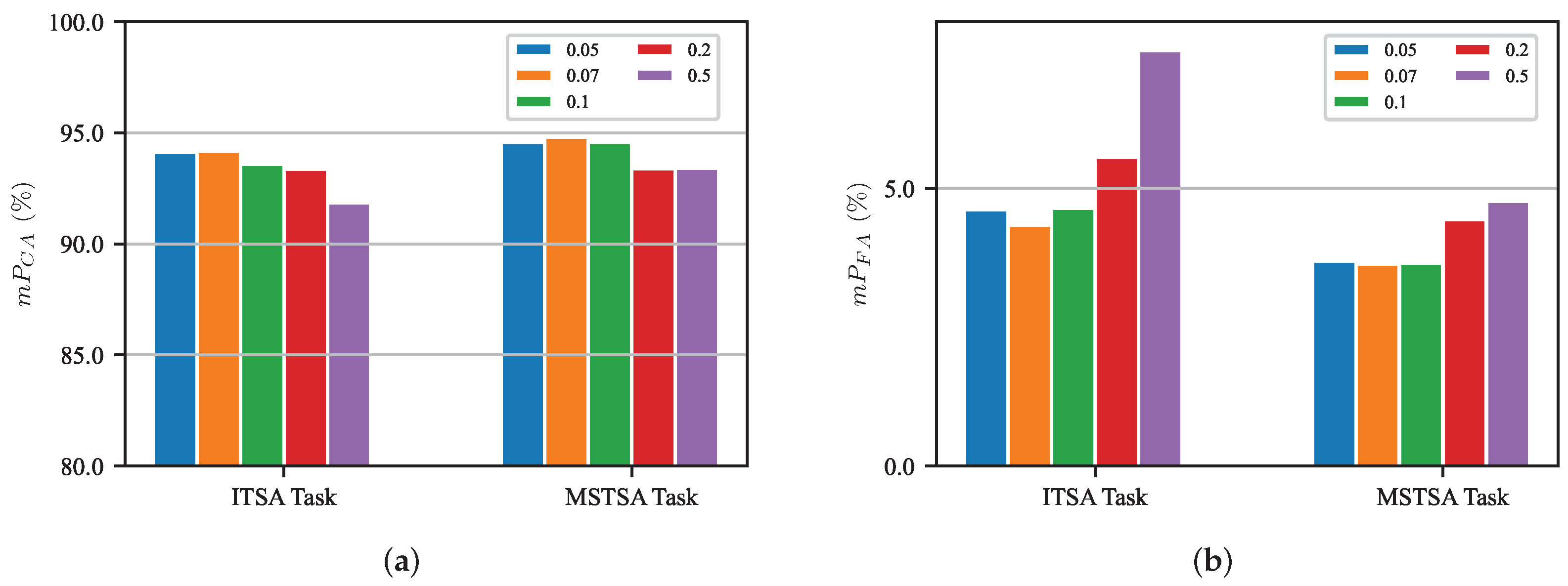
Effect of contrastive loss temperature. The temperature parameter τ plays a crucial role in controlling similarity scaling during contrastive learning. Different temperature settings affect the smoothness or sharpness of similarity distributions, as described in Section 3.5. By tuning this parameter, we can effectively manage how close or distant the positive and negative samples are in the feature space, which significantly affects the model’s performance. Our experiments show that changing the temperature parameter from 0.05 to 1.0 leads to worse model performance, as shown in Figure 13. Conversely, smaller temperature parameters help the model to learn better features, with the optimal value being 0.07.

6. Discussion

Although the two-stage online association algorithm combined with the TSA-cTFER network has achieved good results, there are still some problems and areas for improvement. In this section, we first analyze the performance of TSA-cTFER in a complex association scenario characterized by multiple adjacent track segments. We then discuss the shortcomings of the TSA-cTFER and suggest possible avenues for future improvement.

6.1. Analysis of a Failure Scenario

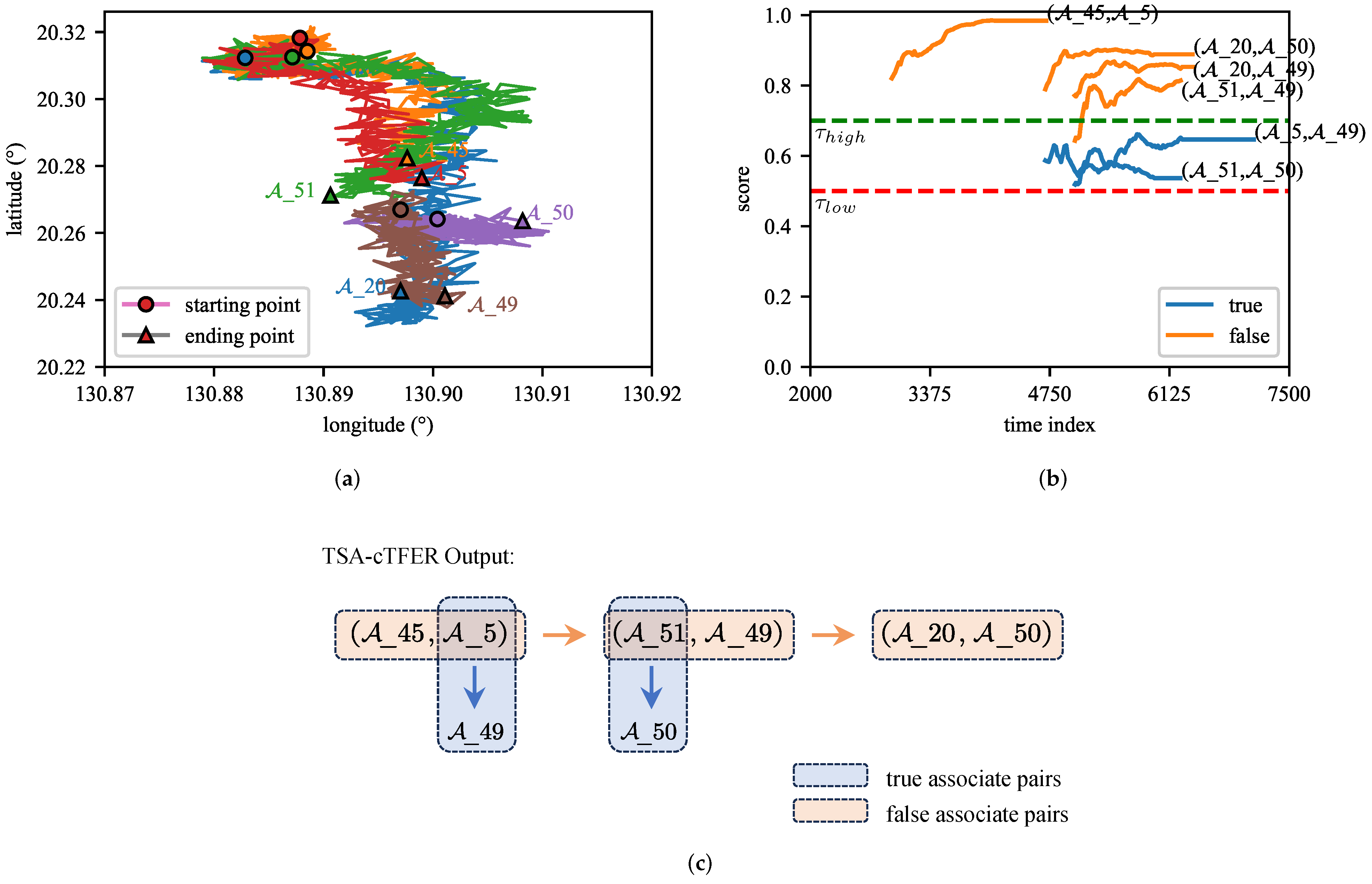
In this challenging association scenario, as shown in Figure 14, multiple adjacent track segments lead to a high probability of misjudgment by the TSA-cTFER. Such misjudgments can significantly impact subsequent determinations of association pairs, resulting in the propagation of association errors. Specifically, the trajectories of the targets in the scene, illustrated in Figure 14a, show that the distances between the targets are very close and their motion patterns are similar. This similarity complicates the process of determining which track segments belong to the same target. The scores of various association pairs computed by TSA-cTFER over time, as depicted in Figure 14b, indicate that in this scenario, the scores for false associations surpass those for true ones. Consequently, the model outputs false associations such as A _ 45 , A _ 5 , A _ 51 , A _ 49 , and A _ 20 , A _ 50 . Furthermore, Figure 14c provides a schematic representation of the propagation of association errors. Initially, the model identifies the association pair A _ 45 , A _ 5 as valid. Due to the one-to-one association constraint, it does not pair A _ 5 with its true associated track A _ 49 . Subsequently, A _ 49 is paired with A _ 51 , further restricting A _ 51 from pairing with A _ 50 . Ultimately, A _ 50 can only be paired with A _ 20 .
This situation leads the model to assign excessively high scores to false association pairs. As illustrated in Figure 14a, there is significant overlap between the track segments A _ 45 and A _ 5 . Moreover, as discussed in Section 5.4.1, we utilized only the latitude and longitude position information during training; other data features, such as heading angle and speed, were excluded due to inaccuracies in the dataset. As a result, from the perspective of model input, the trajectory information exhibits considerable similarity, which can further mislead the model’s associations. Furthermore, we assess similarity based on the distance between feature vectors, processing each trajectory independently through the network. For efficiency reasons, we chose not to implement a framework that concatenates and jointly processes the two trajectories, which restricts the model’s effectiveness in the ITSA task, particularly in scenarios involving numerous similar trajectories.

6.2. Limitations and Future Work

We introduce the TSA-cTFER network to assess trajectory similarity, integrating it with a two-stage online association algorithm to effectively handle interrupted and multi-source track segments. Our experiments show that this approach outperforms existing state-of-the-art deep learning and traditional methods, although some shortcomings remain that require further improvement. To enhance our approach, we consider several key aspects following as:
Data Features and Augumentation: As highlighted in the failure scenarios above, recalculating speed and heading angle based on smoothed latitude and longitude and incorporating these features into the input embedding module of TSA-cTFER could improve the model’s ability to assess trajectory similarity. In addition, as noted in Section 5.4.3, this work has only used random cropping for data augmentation. Exploration of other techniques, such as random masking, may further improve the robustness of the model to meet practical application requirements.
Training Process: Building upon our data preparation strategy described in Section 5.4.1, we mixed the data from all scenarios and then randomly sampled a batch for training. Although this data sampling method proved effective in the early stages of training, it may not provide sufficient meaningful information for the model to learn effectively in the later stages, especially in failure scenarios where multiple similar trajectories exist. Thus, further fine-tuning of the network based on the specific scenarios may be necessary to optimize performance.
End-to-End Association: To achieve online track segment association, we propose a heuristic two-stage online association algorithm that heavily relies on TSA-cTFER’s assessment of trajectory similarity. However, this heuristic algorithm depends on manually defined rules and parameters, limiting its adaptability to different scenarios. Therefore, developing an end-to-end network that integrates trajectory information from the entire scenario and optimizes the association process through deep learning could effectively address these limitations, thereby improving accuracy and significantly reducing the time required for track association.
In summary, addressing these limitations through targeted improvements will enhance the overall performance and applicability of the TSA-cTFER network in real-world scenarios.

7. Conclusions

This paper focuses on addressing the challenges associated with interrupted and multi-source track segment association through a trajectory similarity comparison. The proposed network, TSA-cTFER, exploits the robust representational capabilities of contrastive learning and Transformer Encoder to transform trajectory similarity measurement into distance measurement within high-dimensional vectors. Additionally, in dynamic scenarios where targets continuously appear or disappear, a two-stage online association algorithm is introduced. This algorithm employs different association strategies based on the complexity of the matching trajectories, using M/N logic for easy associations and a delayed strategy for hard pairs. Finally, through the evaluation of real data, the two-stage online association algorithm combined with TSA-cTFER demonstrates excellent results compared to other models, achieving an average accuracy of 94.59% in the ITSA task and an average association accuracy of 94.83% in the MSTSA task, thereby validating the effectiveness of our approach.

Author Contributions

Conceptualization, Z.C. and J.Y.; methodology, Z.C. and J.Y.; software, Z.C.; validation, Z.C., B.L. and J.Y.; formal analysis, B.L.; investigation, Z.C. and J.Y.; resources, H.G.; data curation, B.L.; writing—original draft preparation, Z.C.; writing—review and editing, B.L. and J.Y.; visualization, Z.C., B.L. and J.Y.; supervision, K.T., Z.D., X.L. and H.G.; project administration, H.G.; funding acquisition, J.Y., K.T., Z.D., X.L. and H.G. All authors have read and agreed to the published version of the manuscript.

Funding

This work was supported in part by the National Natural Science Foundation of China under Grant 62001229, Grant 62101264, and Grant 62101260; in part by the Natural Science Foundation of Jiangsu Province under Grant BK20210334 and Grant BK20230915; in part by the China Postdoctoral Science Foundation under Grant 2020M681604 and in part by the Jiangsu Province Postdoctoral Science Foundation under Grant 2020Z441.

Institutional Review Board Statement

Not applicable.

Informed Consent Statement

Not applicable.

Data Availability Statement

The MTAD used in this paper is publicly available at https://jeit.ac.cn/web/data/getData?dataType=Dataset (accessed on 14 December 2023).

Conflicts of Interest

The authors declare no conflicts of interest.

Abbreviations

The following abbreviations are used in this manuscript:
AISAutomatic Identification System
CVConstant Velocity model
CAConstant Acceleration model
CTCoordinated Turn model
CNNConvolutional Neural Network
DTWDynamic Time Warping
EDEuclidean Distance
ITSAInterrupted Track Segment Association
LSTMLong Short-Term Memory
MTADMulti-source Track Association Dataset
MH TSAMultiple Hypothesis Track segment association
MF 2-D TSAMulti-Frame 2-D Track segment association
MSTSAMulti-Source Track Segment Association
TSATrack Segment Association
TSADCNNTSA with Dual Contrast Neural Network
TGRATrack Graph Representation Association
TSA-cTFERTSA-contrastive TransFormer Encoder Representation Network

References

  1. Raghu, J.; Srihari, P.; Tharmarasa, R.; Kirubarajan, T. Comprehensive Track Segment Association for Improved Track Continuity. IEEE Trans. Aerosp. Electron. Syst. 2018, 54, 2463–2480. [Google Scholar] [CrossRef]
  2. Wei, X.; Pingliang, X.; Yaqi, C. Unsupervised and interpretable track-to-track association based on homography estimation of radar bias. IET Radar Sonar Nav. 2024, 18, 294–307. [Google Scholar] [CrossRef]
  3. Yeom, S.W.; Kirubarajan, T.; Bar-Shalom, Y. Track segment association, fine-step IMM and initialization with Doppler for improved track performance. IEEE Trans. Aerosp. Electron. Syst. 2004, 40, 293–309. [Google Scholar] [CrossRef]
  4. Zhang, S.; Bar-Shalom, Y. Track Segment Association for GMTI Tracks of Evasive Move-Stop-Move Maneuvering Targets. IEEE Trans. Aerosp. Electron. Syst. 2011, 47, 1899–1914. [Google Scholar] [CrossRef]
  5. Lin, Q.; Hai-peng, W.; Wei, X.; Kai, D. Track segment association algorithm based on multiple hypothesis models with priori information. J. Syst. Eng. Electron. 2015, 37, 732–739. [Google Scholar] [CrossRef]
  6. Kuhn, H.W. The Hungarian method for the assignment problem. Nav. Res. Logist. Q. 1955, 2, 83–97. [Google Scholar] [CrossRef]
  7. Tian, W.; Wang, Y.; Shan, X.; Yang, J. Track-to-Track Association for Biased Data Based on the Reference Topology Feature. IEEE Signal Process. Lett. 2014, 21, 449–453. [Google Scholar] [CrossRef]
  8. Zhu, H.; Wang, W.; Wang, C. Robust track-to-track association in the presence of sensor biases and missed detections. Inform. Fusion 2016, 27, 33–40. [Google Scholar] [CrossRef]
  9. Zhao, H.; Sha, Z.; Wu, J. An improved fuzzy track association algorithm based on weight function. In Proceedings of the IEEE 2nd Advanced Information Technology, Electronic and Automation Control Conference (IAEAC), Chongqing, China, 25–26 March 2017; pp. 1125–1128. [Google Scholar] [CrossRef]
  10. Wei, X.; Xu, P.; Cui, Y.; Xiong, Z.; Lv, Y.; Gu, X. Track Segment Association with Dual Contrast Neural Network. IEEE Trans. Aerosp. Electron. Syst. 2022, 58, 247–261. [Google Scholar] [CrossRef]
  11. Hochreiter, S.; Schmidhuber, J. Long short-term memory. Neural Comput. 1997, 9, 1735–1780. [Google Scholar] [CrossRef]
  12. Wei, X.; Xu, P.; Cui, Y.; Xiong, Z.; Gu, X.; Lv, Y. Track Segment Association via track graph representation learning. IET Radar Sonar Nav. 2021, 15, 1458–1471. [Google Scholar] [CrossRef]
  13. Jin, B.; Tang, Y.; Zhang, Z.; Lian, Z.; Wang, B. Radar and AIS Track Association Integrated Track and Scene Features Through Deep Learning. IEEE Sens. J. 2023, 23, 8001–8009. [Google Scholar] [CrossRef]
  14. Vaswani, A.; Shazeer, N.; Parmar, N.; Uszkoreit, J.; Jones, L.; Gomez, A.N.; Kaiser, Ł.; Polosukhin, I. Attention is all you need. Proc. Adv. Neural Inf. Process. Syst. 2017, 30. [Google Scholar]
  15. Glorot, X.; Bordes, A.; Bengio, Y. Deep sparse rectifier neural networks. In Proceedings of the 14th International Conference on Artificial Intelligence and Statistics, Ft. Lauderdale, FL, USA, 11–13 April 2011; pp. 315–323. [Google Scholar]
  16. He, K.; Zhang, X.; Ren, S.; Sun, J. Deep residual learning for image recognition. In Proceedings of the IEEE Conference on Computer Vision and Pattern Recognition (CVPR), Las Vegas, NV, USA, 27–30 June 2016; pp. 770–778. [Google Scholar]
  17. Ba, J.L.; Kiros, J.R.; Hinton, G.E. Layer Normalization. arXiv 2016, arXiv:1607.06450. [Google Scholar]
  18. Dosovitskiy, A.; Beyer, L.; Kolesnikov, A.; Weissenborn, D.; Zhai, X.; Unterthiner, T.; Dehghani, M.; Minderer, M.; Heigold, G.; Gelly, S.; et al. An Image is Worth 16 × 16 Words: Transformers for Image Recognition at Scale. In Proceedings of the 9th International Conference on Learning Representations (ICLR), Virtual, Austria, 3–7 May 2021. [Google Scholar]
  19. Hendrycks, D.; Gimpel, K. Gaussian error linear units. arXiv 2016, arXiv:1606.08415. [Google Scholar]
  20. Devlin, J.; Chang, M.W.; Lee, K.; Toutanova, K. BERT: Pre-training of Deep Bidirectional Transformers for Language Understanding. In Proceedings of the NAACL HLT—Conference of the North American Chapter of the Association for Computational Linguistics, Minneapolis, MN, USA, 2–7 June 2019; Volume 1, pp. 4171–4186. [Google Scholar]
  21. Oord, A.v.d.; Li, Y.; Vinyals, O. Representation learning with contrastive predictive coding. arXiv 2018, arXiv:1807.03748. [Google Scholar]
  22. Chen, T.; Kornblith, S.; Norouzi, M.; Hinton, G. A simple framework for contrastive learning of visual representations. In Proceedings of the 37th International Conference on Machine Learning, Virtual, 13–18 July 2020; pp. 1597–1607. [Google Scholar]
  23. Yaqi, C.; Pingliang, X.; Cheng, G.; Zhouchuan, Y.; Jianting, Z.; Hongbo, Y.; Kai, D. Multisource Track Association Dataset Based on the Global AIS. J. Electron. Inf. Techn. 2023, 45, 746–756. [Google Scholar] [CrossRef]
  24. Multi-Source Track Association Dataset. Available online: https://jeit.ac.cn/web/data/getData?dataType=Dataset (accessed on 23 April 2024).
  25. Agrawal, R.; Faloutsos, C.; Swami, A. Efficient similarity search in sequence databases. In Proceedings of the International Conference on Foundations of Data Organization and Algorithms, Chicago, IL, USA, 13–15 October 1993; pp. 69–84. [Google Scholar]
  26. Zheng, Y. Trajectory data mining: An overview. ACM Trans. Intell. Syst. Technol. 2015, 6, 1–41. [Google Scholar] [CrossRef]
  27. Hu, D.; Chen, L.; Fang, H.; Fang, Z.; Li, T.; Gao, Y. Spatio-Temporal Trajectory Similarity Measures: A Comprehensive Survey and Quantitative Study. arXiv 2023, arXiv:2303.05012. [Google Scholar] [CrossRef]
  28. Xu, K.; Hu, W.; Leskovec, J.; Jegelka, S. How powerful are graph neural networks? arXiv 2018, arXiv:1810.00826. [Google Scholar]
  29. Kipf, T.N.; Welling, M. Semi-supervised classification with graph convolutional networks. arXiv 2016, arXiv:1609.02907. [Google Scholar]
  30. Velickovic, P.; Cucurull, G.; Casanova, A.; Romero, A.; Lio, P.; Bengio, Y. Graph Attention Networks. In Proceedings of the International Conference on Learning Representations, Vancouver, BC, Canada, 30 April–3 May 2018. [Google Scholar]
  31. Kingma, D.P.; Ba, J. Adam: A Method for Stochastic Optimization. arXiv 2017, arXiv:1412.6980. [Google Scholar]
  32. Loshchilov, I.; Hutter, F. SGDR: Stochastic Gradient Descent with Warm Restarts. In Proceedings of the 5th International Conference on Learning Representations, Toulon, France, 24–26 April 2016. [Google Scholar]
  33. Srivastava, N.; Hinton, G.; Krizhevsky, A.; Sutskever, I.; Salakhutdinov, R. Dropout: A simple way to prevent neural networks from overfitting. J. Mach. Learn. Res. 2014, 15, 1929–1958. [Google Scholar]
  34. Paszke, A.; Gross, S.; Massa, F.; Lerer, A.; Bradbury, J.; Chanan, G.; Killeen, T.; Lin, Z.; Gimelshein, N.; Antiga, L.; et al. PyTorch: An Imperative Style, High-Performance Deep Learning Library. Adv. Neural Inf. Process. Syst. 2019, 32, 8024–8035. [Google Scholar]
  35. Reimers, N.; Gurevych, I. Sentence-BERT: Sentence Embeddings using Siamese BERT-Networks. In Proceedings of the EMNLP-IJCNLP—Conference on Empirical Methods in Natural Language Processing and 9th International Joint Conference on Natural Language Processing, Hong Kong, China, 3–7 November 2019; pp. 3982–3992. [Google Scholar]
Figure 1. TSA-cTFER network overview. This figure illustrates the process of extracting features from track segments using TSA-cTFER, and compares these features to assess the similarity between track segments, thereby determining whether they originate from the same target. The scenario trajectory data include interrupted track segments, such as T 1 A and T 2 A , or multi-source track segments, such as T 1 A and T 4 B . After processing by TSA-cTFER, each track segment acquires high-dimensional feature representations ( z i , i = 1 , , 4 ). Track segments originating from the same target are defined as positive pairs, e.g., ( z 1 , z 4 ) and ( z 1 , z 2 ) , while all others are categorized as negative pairs. Through contrastive learning, the network continuously minimizes distances between positive samples and maximizes distances between negative samples to achieve effective track segment association.
Remotesensing 16 03380 g001
Figure 2. The overall framework of TSA-cTFER. (a) The TSA-cTFER network comprises an input embedding module, a Transformer encoder module, and an output pooling module. For the two distinct tasks, ITSA and MSTSA, a shared feature extraction module is utilized; however, each task employs different output heads to derive trajectory features. (b) Input Embedding Module. Different attributes of the targets, both continuous x c and discrete x d , are converted into a unified vector representation x ^ for easier processing by the network. (c) Transformer Encoder. Given the discrete points of the trajectory, the Transformer Encoder employs a multi-head attention mechanism to extract relationships among these trajectory points.
Remotesensing 16 03380 g002
Figure 3. Construction of positive and negative association pairs. The scene contains two targets and two sources, with tracks from different sources represented in distinct colors. Different dotted arrows indicate association pairs, with red for positive pairs and black for negative pairs.
Remotesensing 16 03380 g003
Figure 4. Diagram of the two-stage online association algorithm for TSA. Sensors A and B continuously report target positions and other relevant information. The Track State Update Module gathers these target states and employs TSA-cTFER to compute their features. The Two-Stage Association module calculates the similarity between association pairs based on the features of the tracks, employing a staged association strategy to achieve pairing among the targets.
Remotesensing 16 03380 g004
Figure 5. The selection process of invalid/easy/hard association pairs.
Remotesensing 16 03380 g005
Figure 6. Four typical scenarios in MTAD. Tracks reported from different sources are plotted using different colors.
Remotesensing 16 03380 g006
Figure 7. The variation of association scores. (a) A scenario of association of tracks in the MTAD. Different colors represent the trajectories of different targets. (b) The variation of association scores over time in ITSA. (c) The variation of association scores over time in MSTSA.
Remotesensing 16 03380 g007
Figure 8. Effect of different pooling strategies. (a) m P CA variation for different pooling strategies. (b) m P FA variation for different pooling strategies.
Remotesensing 16 03380 g008
Figure 9. Effect of different input trajectory length. (a) m P CA and m P FA variation in the ITSA Task. (b) m P CA and m P FA variation in the MSTSA Task.
Remotesensing 16 03380 g009
Figure 10. Effect of hidden state size.
Remotesensing 16 03380 g010
Figure 11. Effect of the number of layers.
Remotesensing 16 03380 g011
Figure 12. Effect of training batch size. (a) m P CA and m P FA variation in the ITSA Task. (b) m P CA and m P FA variation in the MSTSA Task.
Remotesensing 16 03380 g012
Figure 13. Effect of different contrastive loss temperatures. (a) m P CA variation for different contrastive loss temperatures. (b) m P FA variation for different contrastive loss temperatures.
Remotesensing 16 03380 g013
Figure 14. A failure scenario in the ITSA task. (a) Movement trajectories of targets within the scene. Different colors represent the trajectories of different targets. (b) Scores of various association pairs over time. (c) Example of incorrect association pairs outputted by TSA-cTFER and the propagation of association errors.
Remotesensing 16 03380 g014
Table 1. Results of Interrupted Track Segment Association.
#params. (M) mP CA (%) mP FA (%) mT AP (s) mwP CA (%) mwP FA (%) mwT AP (s)
ED-based TSA-48.8755.5986.9227.9875.0579.44
MH TSA [5]-93.796.3549.3490.8711.9943.42
MF 2-D TSA [1]-80.545.30156.8275.739.92132.59
TSADCNN (Sep.) [10]0.90879.41 ± 3.036.61 ± 0.59227.27 ± 23.2476.70 ± 2.6612.14 ± 0.74212.43 ± 15.62
TSADCNN [10]1.30183.86 ± 0.135.52 ± 0.24201.01 ± 13.6380.82 ± 0.1510.85 ± 0.05189.51 ± 2.17
TGRA (Sep.) [12]0.53485.64 ± 0.728.63 ± 0.27152.71 ± 8.6879.55 ± 0.6216.16 ± 0.23153.70 ± 1.26
TGRA [12]0.53485.02 ± 0.299.02 ± 0.07160.85 ± 10.7679.55 ± 0.1816.17 ± 0.11150.42 ± 1.00
TSA-cTFER (Sep.)0.67094.21 ± 0.053.46 ± 0.06130.91 ± 1.1390.77 ± 0.097.39 ± 0.07139.19 ± 0.96
TSA-cTFER0.67494.59 ± 0.043.49 ± 0.08131.00 ± 9.4991.29 ± 0.137.34 ± 0.15136.13 ± 2.97
The best results are bolded.
Table 2. Results of Multi-source Track Segment Association.
#params. (M) mP CA (%) mP FA (%) mT AP (s) mwP CA (%) mwP FA (%) mwT AP (s)
ED-based TSA-50.9925.85464.3839.3039.86247.04
DTW-based TSA-54.2441.77505.5235.2760.56638.35
TSADCNN (Sep.) [10]0.90894.68 ± 0.512.73 ± 0.40235.85 ± 6.7491.80 ± 0.945.13 ± 0.70269.29 ± 11.55
TSADCNN [10]1.30192.85 ± 0.224.22 ± 0.22259.49 ± 2.1385.36 ± 0.308.05 ± 0.27311.86 ± 3.01
TGRA (Sep.) [12]0.53493.81 ± 0.133.41 ± 0.11252.84 ± 1.5290.03 ± 0.426.47 ± 0.38303.85 ± 3.13
TGRA [12]0.53491.61 ± 0.135.32 ± 0.11271.25 ± 2.2685.60 ± 0.3110.59 ± 0.27334.80 ± 2.54
TSA-cTFER (Sep.)0.67094.83 ± 0.382.61 ± 0.34234.65 ± 1.1092.20 ± 0.524.79 ± 0.47269.79 ± 2.01
TSA-cTFER0.67494.25 ± 0.093.06 ± 0.11246.95 ± 0.7891.00 ± 0.125.75 ± 0.11290.20 ± 1.47
Disclaimer/Publisher’s Note: The statements, opinions and data contained in all publications are solely those of the individual author(s) and contributor(s) and not of MDPI and/or the editor(s). MDPI and/or the editor(s) disclaim responsibility for any injury to people or property resulting from any ideas, methods, instructions or products referred to in the content.