Comparison of Soil Water Content from SCATSAR-SWI and Cosmic Ray Neutron Sensing at Four Agricultural Sites in Northern Italy: Insights from Spatial Variability and Representativeness

Abstract

Monitoring soil water content (SWC) is vital for various applications, particularly in agriculture. This study compares SWC estimated by means of SCATSAR-SWI remote sensing (RS) at different depths (T-values) with Cosmic Ray Neutron Sensing (CRNS) across four agricultural sites in northern Italy. Additionally, it examines the spatial mismatch and representativeness of SWC products’ footprints based on different factors within the following areas: the Normalized Difference Vegetation Index (NDVI), soil properties (sand, silt, clay, Soil Organic Carbon (SOC)), and irrigation information. The results reveal that RS-derived SWC, particularly at T = 2 depth, exhibits moderate positive linear correlation (mean Pearson correlation coefficient, R = 0.6) and a mean unbiased Root–Mean–Square Difference (ubRMSD) of 14.90%SR. However, lower agreement is observed during summer and autumn, attributed to factors such as high biomass growth. Sites with less variation in vegetation and soil properties within RS pixels rank better in comparing SWC products. Although a weak correlation (mean R = 0.35) exists between median NDVI differences of footprints and disparities in SWC product performance metrics, the influence of vegetation greenness on the results is clearly identified. Additionally, RS pixels with a lower percentage of sand and SOC and silt loam soil type correlate to decreased agreement between SWC products. Finally, localized irrigation practices also partially explain some differences in the SWC products. Overall, the results highlight how RS pixel variability of the different factors can explain differences between SWC products and how this information should be considered when selecting optimal ground-based measurement locations for remote sensing comparison.

1. Introduction

Soil water content (SWC) plays a pivotal role in various applications, particularly in agriculture [1]. The amount of water available to plants is directly influenced by SWC [2], making its monitoring essential for tasks such as planning irrigation, predicting crop yield, and ensuring food safety [3]. Despite its critical importance, tracking SWC poses substantial challenges due to its temporal and strong spatial variability [4]. This variability is driven by a combination of natural hydrological processes at the land surface [5] and human activities like irrigation and drainage [6].

Today, an array of tools is available for monitoring SWC, ranging from localized point-scale measurements to advanced large-scale remote sensing (RS) techniques [7]. RS methods have gained immense popularity due to their capacity to cover large areas and inaccessible or hard-to-reach regions [8]. Despite the increasing availability of RS products, a key aspect is still the need for ground observations for the assessment and the understanding of the value of the signal in the different applications [9,10].

Recognizing this need, an International Soil Moisture Network (ISMN) has been established, progressively expanding with the integration of new technologies to cover broader geographical areas [11,12]. However, the assessment of SWC at agricultural sites within this network is still somewhat limited due to the high cost of deploying enough stations within a satellite footprint to produce accurate estimates of SWC in specific areas [13]. Recently, there has been an increased focus on developing and assessing proximal SWC sensors [14]. These non-invasive detectors, located near the ground, offer benefits such as the capability to measure SWC at sub-daily intervals on an intermediate scale (within a radius of 10 to 200 m) and down to most of the root depth (e.g., 50 cm), which opens up new possibilities for hydrological research in the agricultural field scale [15]. Among the various non-invasive methods, Cosmic Ray Neutron Sensing (CRNS) [16] has shown reliable performance in different situations [17,18,19,20]. Unlike the difference in depth range covered [21,22], the use of CRNS for RS assessments has been explored in several studies, taking advantage of its benefits, such as recording long-term series with minimal maintenance requirements [23,24,25].

While CRNS covers a larger area compared to point-scale measurements, there still exists a spatial misalignment between CRNS and RS products, with resolutions varying from hundreds of meters to tens of kilometers. For instance, the SWC product derived from Sentinel-1 at 1 km resolution [26,27] falls into the former category, while ASCAT [28] belongs to the latter. Consequently, it is essential to grasp the spatial representativeness of ground SWC observations for an accurate assessment [29].

In this research, our objective is to compare the SCATSAR-SWI, a combined RS product for daily SWC at different depths at a kilometer scale, to SWC measured by CRNS across four agricultural sites in northern Italy. The Soil Water Index (SWI) developed by the Copernicus Global Land Service (CGLS) is derived from the integration of 25 km ASCAT Surface Soil Moisture (SSM) [28] and 1 km Sentinel-1 SSM [30] products. This fusion results in a globally covered, high spatiotemporal product, enhancing our understanding of soil water dynamics [31]. Furthermore, point-scale SWC measurements collected during Time Domain Reflectometry (TDR) campaigns at the specified four locations are used to enhance the evaluation of the estimates obtained from the different products.

To evaluate the spatial representativeness of the ground measurements more comprehensively, we initially utilized the Normalized Difference Vegetation Index (NDVI) as an indicator of vegetation vigor and biomass, shedding light on the correlation between vegetation dynamics and the agreement between the soil water content time series [32,33]. Additionally, we investigated soil physical parameters, including sand, silt, and clay, alongside Soil Organic Carbon (SOC). These properties were selected based on previous studies indicating their significant relationship with SWC values [33,34]. Finally, the irrigation information within CRNS footprints at two experimental sites is analyzed to assess the effect of agricultural water use on SWC variability and to interpret the possible differences between the observations.

2. Materials and Methods

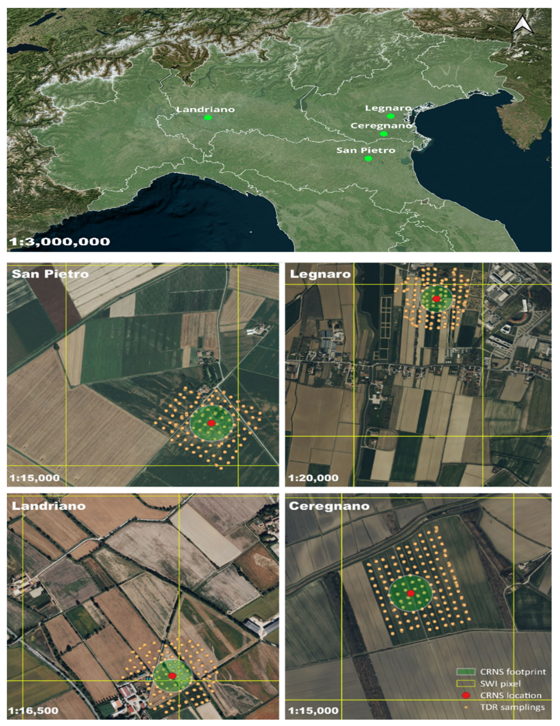
2.1. Experimental Sites

Observations collected at four experimental sites in the Po River Plain in northern Italy were used for the comparison (Figure 1). For details about the sites and CRNS performances, we refer to the study of Ref. [20]. Here, we summarize the main characteristics relevant to interpreting the results. Specifically, the CRNS sensors were placed over low-biomass grasslands flanked by agriculturally farmed fields at the San Pietro (44.65N, 11.64E) and Legnaro locations (45.34N, 11.96E). In contrast, the CRNS sensors were placed in the middle of agricultural fields where rapid biomass growth and irrigation occurred in Ceregnano (45.05N, 11.86E) and Landriano (45.31N, 9.26E). More precisely, a sprinkler system was used at Landriano to both cultivate and irrigate sorghum, and a variable-rate irrigation ranger system was used at Ceregnano to cultivate and water soybeans. The majority of the sensor-investigated regions have relatively uniform soil texture, with the exception of Ceregnano, where a sandy fluvial deposit crosses the loamy field. At each location, meteorological stations administered by the Regional Environmental Protection Agencies (ARPA) gathered weather data (namely precipitation) at the same locations as the CRNS sensors or at a short distance apart (a few kilometers). In these instances, the meteorological readings are considered to reflect the local conditions [20].

2.2. Ground Measurements

2.2.1. Cosmic Ray Neutron Sensing (CRNS)

CRNS is a non-invasive technique employed for measuring SWC across intermediate-scale areas [16]. In this study, we utilized observations from CRNS-FINAPP3 sensors (https://www.finapptech.com/en/, accessed on 10 December 2023). These sensors, detailed in Ref. [20], operate by measuring neutron count rates, which are then transformed into Volumetric Water Content (VWC). Standard corrections to account for variations in atmospheric pressure, air humidity, and incoming neutron variability are first performed. Then, these CRNS devices underwent calibration based on three independent soil sampling gravimetric campaigns for each site; this calibration approach, consistent with studies by Refs. [35,36], enhances the accuracy of CRNS measurements, aligning them with ground truth data obtained through direct soil sampling. The CRNS sensors were operational at all four sites for almost the entire vegetation season of 2021, spanning from March to December, except San Pietro, which extended from March to September. The few gaps in the time series were due to the low power supply by the solar panel. For more details about the CRNS calibration and data processing, readers can refer to Ref. [20].

The footprint of CRNS is reasonable for many agricultural field-scale applications, although the area cannot be defined exactly since the sensitivity of the sensor decreases by increasing the radius. According to a detailed study [35], 120 m, equivalent to an area of almost 5 hectares, would be a reasonable assumption to account for the major contribution (86%) of CRNS footprint in the fields where the situation alternates between wet and humid conditions. In this present study, a radius of 125 m was considered (Figure 1). The penetration soil depth of the CRNS signal varies between 10 and 50 cm, also depending on soil water content but with higher sensitivity to the upper soil layers. Following the procedure described by Ref. [35], the average penetration depth at the four sites has been estimated to be around 20 cm, i.e., deeper than the expected RS penetration depth. For this reason, even though studies show that CRNS is highly suitable for validating satellite soil moisture products because both RS sensors and CRNS are most responsive to the top few centimeters of soil [37], and CRNS SWC is compared to the RS product extrapolated to deeper depths using the exponential filter [2].

To enhance comparability among SWC products, RS value, expressed in the degree of saturation (SR), is usually transformed to VWC matching the mean and variance of ground-based and RS time series; e.g., Ref. [31]. Ground-based values are, however, uncertain at the remote sensing scale (1 km²) and could introduce relevant errors. Furthermore, relatively longer time series (e.g., >one year) are needed for representative mean and variance values. For this reason, in this present study, we converted CRNS VWC to %SR based on soil properties measured in soil samples collected over the CRNS footprint. Specifically, for Ceregnano and San Pietro, the conversion utilized bulk density and porosity of the soil at the study sites, employing Equations (1) [38] and (2) [39], where φ, ρ_bd [g/cm³], and 2.65 indicate porosity, soil bulk density, and average particle density, respectively. Moreover, s and r express saturated and residual values of the SWC in VWC% ($\theta$). To obtain SWC in SR, assumptions of ${\theta }_r$ = 0 and ${\theta }_s$ = $\mathsf{\phi }$ were considered. On the other hand, for Landriano and Legnaro, since the maximum observed hourly CRNS VWC was higher than the porosity extracted by Equation (1), we considered ${\theta }_s$ in Equation (2) to be equal to the maximum measured amount of their hourly CRNS data.

$$\mathsf{\phi }=1-{\displaystyle \frac{{\rho }_{\mathrm{bd}}}{2.65}}$$

(1)

$$\mathrm{S}\mathrm{R}={\displaystyle \frac{\theta -{\theta }_r}{{\theta }_s-{\theta }_r}}$$

(2)

Finally, to maintain uniform temporal resolution across datasets, CRNS values were converted to daily averages; this adjustment ensures consistency in the comparison and analysis of SWC dynamics over time.

2.2.2. Soil Moisture Surveys with Point-Scale Soil Moisture Sensor (TDR)

Additionally, for improved assessment of the SWC estimates, on-site point-scale SWC measurements obtained through TDR campaigns conducted at the designated four locations have been conducted. TDR is a point-scale method for SWC retrieval, functioning on the principle of measuring the time taken for an electromagnetic pulse to travel along a sensor rod inserted into the soil and reflect back. The mechanism relies on the dielectric properties of the soil, allowing for the determination of SWC at the sensed depth [40,41]. For this research, a mobile TDR device was utilized (product manual: https://www.specmeters.com/documents, FieldScout-TDR350, accessed on 20 August 2024). This choice allowed for flexibility in the field, enabling the collection of point-scale measurements at different locations within the agricultural sites.

Three campaigns were conducted at each site to ensure comprehensive data collection. The results of these surveys are summarized in

Table 1. Information acquired at the different experimental sites in 2021. SWC in VWC% acquired by TDR device and SWC in %SR, achieved using conversion steps; ρ_bd and φ are the soil bulk density and porosity for each date, respectively.

Site	Campaign Date	ρbd [g/cm3]	SWC [VWC%]	φ	SWC [%SR]
San Pietro	15 March	1.384	15.59 ± 4.58	0.478	32.63
	10 May	1.373	15.66 ± 6.44	0.482	32.50
	19 July	1.295	6.69 ± 2.61	0.511	13.08
Legnaro	29 March	1.409	20.59 ± 4.81	0.468	43.97
	26 May	1.421	33.89 ± 4.18	0.464	73.07
	3 August	1.336	12.02 ± 5.35	0.496	24.24
Landriano	22 March	1.322	17.8 ± 5.57	0.501	35.52
	17 May	1.285	13.23 ± 4.18	0.515	25.68
	29 July	1.295	10.46 ± 5.48	0.511	20.46
Ceregnano	10 March	1.397	24.8 ± 6.86	0.473	52.45
	31 May	1.306	16.53 ± 4.23	0.507	32.59
	15 July	1.386	17.86 ± 7.45	0.477	37.44

. A fixed rod length of 5 cm was maintained for the TDR device to guarantee relatively equal conditions in terms of sensed depth by RS. Nested sampling (regular grid of 30–40 m and five measurements at each grid point) was implemented around the CRNS location during TDR campaigns (see Figure 1). Each campaign involved a minimum of 500 measurements, providing a robust dataset for comparison purposes. The average value for each date and site was calculated to represent the daily average. The decision to use daily average values for the TDR surveys and CRNS observations was made to enable effective comparison with the RS product. The TDR surveys were conducted during a specific time frame, while CRNS observations were aggregated at a daily time resolution to align with the RS product. The average footprint of the areas where TDR measurements were conducted can be estimated at ~12 hectares. The same procedure of unit conversion for CRNS was used for TDR measurements, i.e., Volumetric Water Content by TDR was transformed to saturation (SR) by means of Equations (1) and (2) and soil properties measured in soil samples collected at the CRNS location.

2.3. Remote Sensing Soil Moisture Product (RS)

The SWC product by RS utilized in this research is SCATSAR-SWI, which is a comprehensive indicator of daily soil water content at various depths with a spatial resolution of 1 km². This product is developed by the Copernicus Global Land Service (CGLS), and its fusion strategy involves integrating the data of two active sensors: 25 km ASCAT SSM [28] and 1 km Sentinel-1 SSM [30] products. For a more detailed understanding, refer to the work of Ref. [31] and the official portal of the product: https://land.copernicus.eu/global/products/swi (accessed on 15 November 2023).

This RS product was chosen for our study due to its high spatial and temporal resolution, making it well-suited for agricultural field-scale investigations. It might be prudent to include that 1 km resolution RS products were used in a considerable number of research studies in agricultural contexts, highlighting their capability to provide a satisfactory level of resolution [42,43,44]. The SCATSAR-SWI’s fusion approach capitalizes on the high temporal resolution of ASCAT and the high spatial resolution of Sentinel-1. Despite the attenuation of the Sentinel-1 signal to some extent, the SCATSAR-SWI product benefits from the Sentinel-1 parametrization, ensuring a comprehensive and more accurate representation of SWC dynamics.

The SCATSAR-SWI retrieval method involves characteristic T-values, representing different soil depths based on the approach proposed by Ref. [2]. It is important to note that the SCATSAR-SWI does not consider soil texture in its retrieval process, which influences the relationship between the T-value and soil depth [45]. To offer flexibility to users in selecting the most appropriate data for their needs, eight T-values (2, 5, 10, 15, 20, 40, 60, 100) are provided per product. In our research, we focused on characteristic T-values of 2, 5, and 10, excluding deeper depths since our primary focus is on comparing to the CRNS signal, which is also more sensitive to the upper soil layers [35].

This RS product comes with some quality flags where some problematic surfaces, like frozen ones, are marked. The surfaces other than normal were disregarded during the data processing of SCATSAR-SWI.

2.4. Assessment of the Spatial Variability and Representativeness

The spatial variability of soil water content is driven by several factors like topography, weather and climate conditions, vegetation, and soil properties [46]. The areas investigated in this present study are relatively small and flat. For this reason, the first two factors are negligible, and we focus the analysis on the spatial variability of vegetation and soil. In addition, the effect of irrigation management is investigated based on information provided during the field surveys.

For the assessment of the vegetation, NDVI, a widely used greenness indicator derived from RS data, is utilized. It assesses vegetation presence and health by analyzing near-infrared (NIR) and red (RED) spectral bands. Ranging from −1 to 1, higher values indicate healthier vegetation. NDVI correlates closely with SWC levels, as changes in SWC directly impact vegetation health and NDVI values. Elevated SWC levels typically yield higher NDVI values [47]. Studies in the literature, such as Refs. [48,49], have demonstrated the effectiveness of NDVI as a spatial representativeness indicator.

For each site, NDVI values were achieved using Copernicus Sentinel-2 twin satellite Bottom-of-Atmosphere level (L2A) images for two regions of the study: the area covered by the CRNS and the 1 km resolution pixel of SCATSAR-SWI. The RED and NIR bands of Sentinel-2 have a resolution of 10 m; therefore, the NDVI estimated using these bands from this satellite also has a resolution of 10 m.

The studies were confined to the time frame during which the CRNS were operational at the respective sites. Images with more than 40% cloudy pixels were filtered to ensure data accuracy and sufficiency for analysis. The differences in median NDVI values between the CRNS footprint and remote sensing pixel-wise were investigated to quantify representativeness and spatial mismatches between the CRNS and RS footprints.

For the assessment of the soil variability, SoilGrids (https://soilgrids.org/, accessed on 20 February 2024) was used. This product provides global maps of soil properties with a medium spatial resolution of 250 m cell size [50]. For our study areas, we extracted maps of soil texture (sand, silt, and clay) and Soil Organic Carbon (SOC) because these properties play a fundamental role in determining water distribution, with studies indicating their importance for spatial representativeness [51,52]. Also, for these soil properties, the analysis focuses on the difference between the values within the CRNS footprint and the distributions over the remote sensing pixel.

Finally, inquiries from farmers provide information on the irrigation at Ceregnano and Landriano that has been further explored. The reported irrigation dates for Ceregnano are 22 July and 12 August 2021, while for Landriano is 23 June 2021. The irrigation quantity for all dates and locations is around 20 mm per day. Please note that this value has been assumed based on irrigation methods and communication of the farmers but was not measured.

2.5. Performance Metrics

In this study, to assess the disparity among datasets, two common metrics were employed: (1) Pearson correlation coefficient (R) and (2) unbiased Root–Mean–Square Difference (ubRMSD). The association between ground reference data and product datasets was quantified using R. The utilization of ubRMSD is recommended for estimating the precision of remotely sensed SWC products, as it considers biases in the mean of estimated SWC from both RS and ground-truth data [53]. Equations (3)–(6) are used for the aforementioned aims, where SWC_RS represents satellite SWC retrieval and SWC_CRNS denotes CRNS measurement. N is the total number of data pairs. The covariance of two datasets, denoted as Cov in Equation (3), encompasses the variance of satellite (σ_RS) and CRNS data (σ_CRNS).

$$\mathrm{R}={\displaystyle \frac{\mathrm{C}\mathrm{o}\mathrm{v}({\mathrm{S}\mathrm{W}\mathrm{C}}_{\mathrm{R}\mathrm{S}},{\mathrm{S}\mathrm{W}\mathrm{C}}_{\mathrm{C}\mathrm{R}\mathrm{N}\mathrm{S}})}{{\mathsf{\sigma }}_{\mathrm{R}\mathrm{S}}{\mathsf{\sigma }}_{\mathrm{C}\mathrm{R}\mathrm{N}\mathrm{S}}}}$$

(3)

$$\mathrm{R}\mathrm{M}\mathrm{S}\mathrm{D}=({{\displaystyle \frac{1}{\mathrm{N}}}{\sum }_{\mathrm{i}=1}^{\mathrm{N}}{({\mathrm{S}\mathrm{W}\mathrm{C}}_{\mathrm{R}\mathrm{S}}-{\mathrm{S}\mathrm{W}\mathrm{C}}_{\mathrm{C}\mathrm{R}\mathrm{N}\mathrm{S}})}_{\mathrm{i}}^2)}^{{\displaystyle \raisebox{1ex}{$1$}\!\left/ \!\raisebox{-1ex}{$2$}\right.}}$$

(4)

$$\mathrm{B}\mathrm{i}\mathrm{a}\mathrm{s}={\displaystyle \frac{1}{\mathrm{N}}}{\sum }_{\mathrm{i}=1}^{\mathrm{N}}{({\mathrm{S}\mathrm{W}\mathrm{C}}_{\mathrm{R}\mathrm{S}}-{\mathrm{S}\mathrm{W}\mathrm{C}}_{\mathrm{C}\mathrm{R}\mathrm{N}\mathrm{S}})}_{\mathrm{i}}$$

(5)

$$\mathrm{u}\mathrm{b}\mathrm{R}\mathrm{M}\mathrm{S}\mathrm{D}={{(\mathrm{R}\mathrm{M}\mathrm{S}\mathrm{D}}^2-{\mathrm{B}\mathrm{i}\mathrm{a}\mathrm{s}}^2)}^{{\displaystyle \raisebox{1ex}{$1$}\!\left/ \!\raisebox{-1ex}{$2$}\right.}}$$

(6)

The assessment of SWC products and their spatial mismatch can vary significantly across diverse hydrological conditions and time scales [54]. While various SWC products may capture similar drying and wetting cycles, they may exhibit distinct short-term fluctuations [55]. Therefore, in addition to comparing the raw time series of ground measurements with remotely sensed products, we aim to break down the series into a low-frequency SWC dynamic and a higher-frequency anomaly. The 35-day moving window was utilized based on recommendations for seasonality as suggested in the literature [56,57]. In this method, we derive performance metrics by grouping 35 daily data points [t − 17, t + 17] centered on day t.3.

3. Results

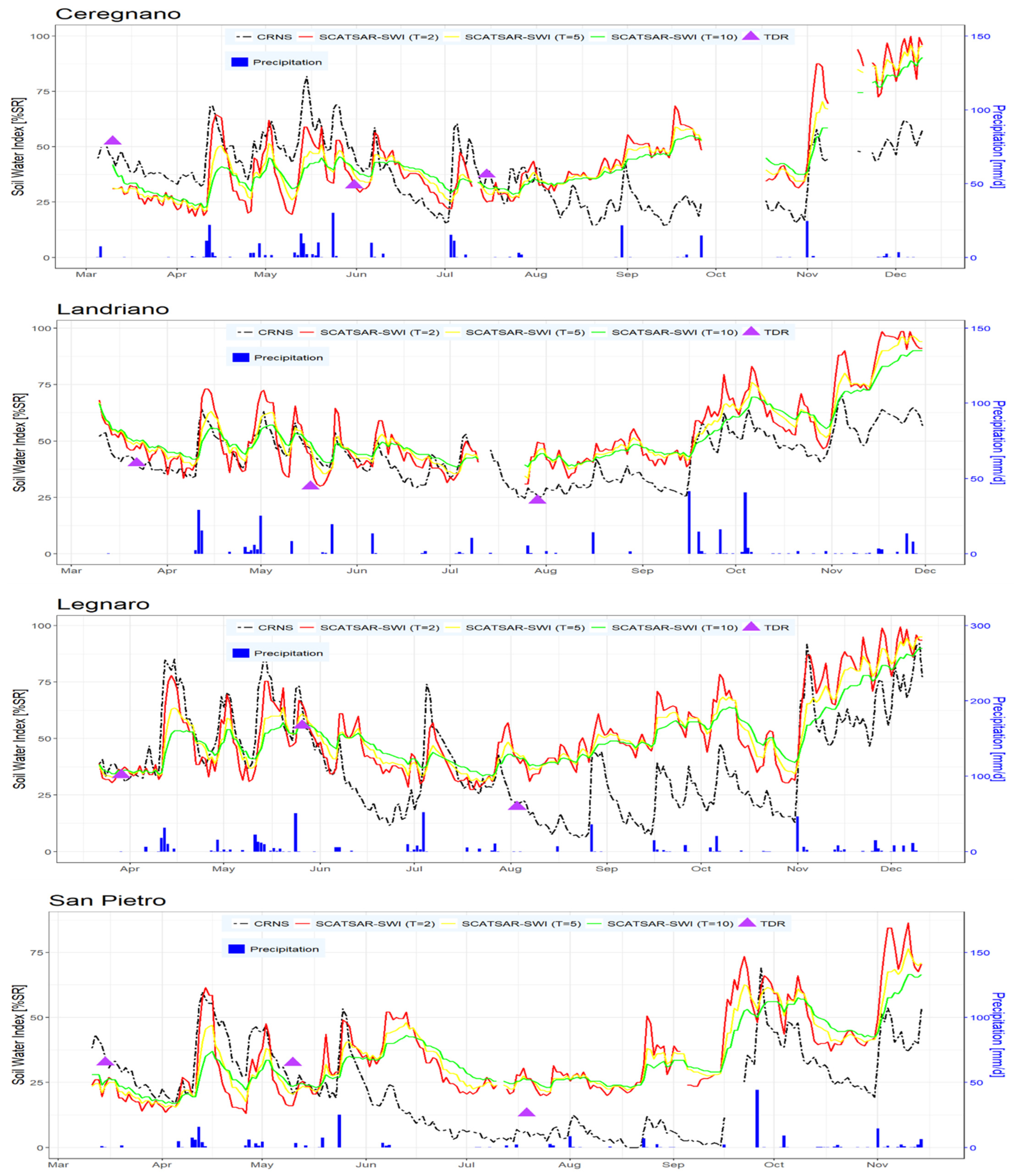
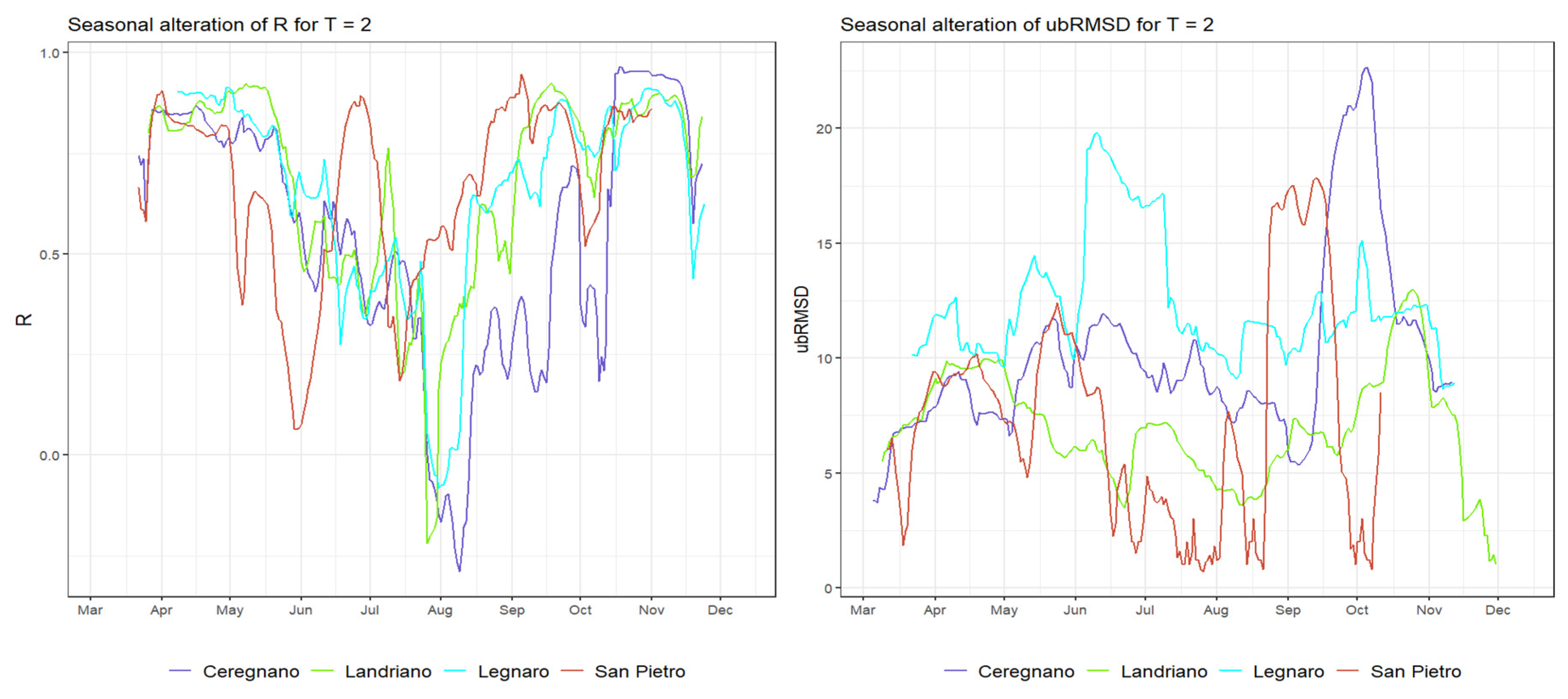
3.1. Comparison of Remote Sensing and CRNS Soil Water Content

The time series of SWI products derived from RS and CRNS are presented in Figure 2. The performance metrics are reported in

Table 2. Performance metrics of different T-values between SWC derived from SCATSAR-SWI product and CRNS for four sites separately and also average amounts for all sites.

Site	T-Values	R	ubRMSD
Ceregnano	T = 2	0.38	19.01
	T = 5	0.31	18.37
	T = 10	0.26	17.40
Landriano	T = 2	0.80 1	10.35 2
	T = 5	0.78	9.41
	T = 10	0.74	8.85
Legnaro	T = 2	0.67	16.36
	T = 5	0.61	17.16
	T = 10	0.54	17.98
San Pietro	T = 2	0.55	13.88
	T = 5	0.53	13.80
	T = 10	0.48	14.05
All sites (mean)	T = 2	0.60 3	14.90 4
	T = 5	0.56	14.68
	T = 10	0.51	14.57

¹ The highest R among sites. ² The lowest ubRMSD among sites when T = 2. ³ Mean R of all sites for T = 2. ⁴ Mean ubRMSD of all sites for T = 2.

. To calculate the metrics, days where data were missing for one sensor were excluded. For instance, as shown in Figure 2, the CRNS instrument in Ceregnano was not operational for approximately 20 days from late September to mid-October. Therefore, both the CRNS and RS data were disregarded during that period. Noteworthy, at all sites, a good agreement between the SWI products is observed with dynamics that well respond to precipitation events. Some differences are captured when looking at the absolute values with CRNS and TDR data exhibiting closer agreement than the RS time series. More specifically, examining the RS-derived time series at different depths (T = 2, T = 5, and T = 10), a general trend emerges, with RS-derived SWI (T = 2) showing greater fluctuation and dynamic alignment with CRNS, suggesting T = 2 to be the best deal of depth for our studied sites when comparing the SCATSAR-SWI product. Considering seasonality, during spring, the time series show more similarities. August onwards (earlier for San Pietro), divergence of values is evident. Entering the winter period, RS-derived SWI tends to be higher than CRNS (although with a favorable dynamic match), indicating potential overestimation of SWC by RS. As an example, the pronounced difference (exceeding 40%SR) is noted for Ceregnano in December.

For T = 2, the mean R and ubRMSD for the four sites are 0.6 and 14.90%SR, respectively (Table 2). These metrics suggest a moderate positive linear relationship between CRNS and RS, with Landriano exhibiting the strongest match (R = 0.80, ubRMSD = 10.35) and Ceregnano the weakest (R = 0.38, ubRMSD = 19.01). The results at T > 2 show, in general, lower performance and only a slight improvement when looking at ubRMSD.

Examining the time series of 35-day window metrics for T = 2 (Figure 3), major and minor declines in correlation during the summer period (especially in August) and December, respectively, are evident. Correlation generally tends to be strong in the spring and autumn seasons. Conversely, the trend of ubRMSD varies across sites, precluding the derivation of a generalized outcome.

3.2. Spatial Variability and Representativeness

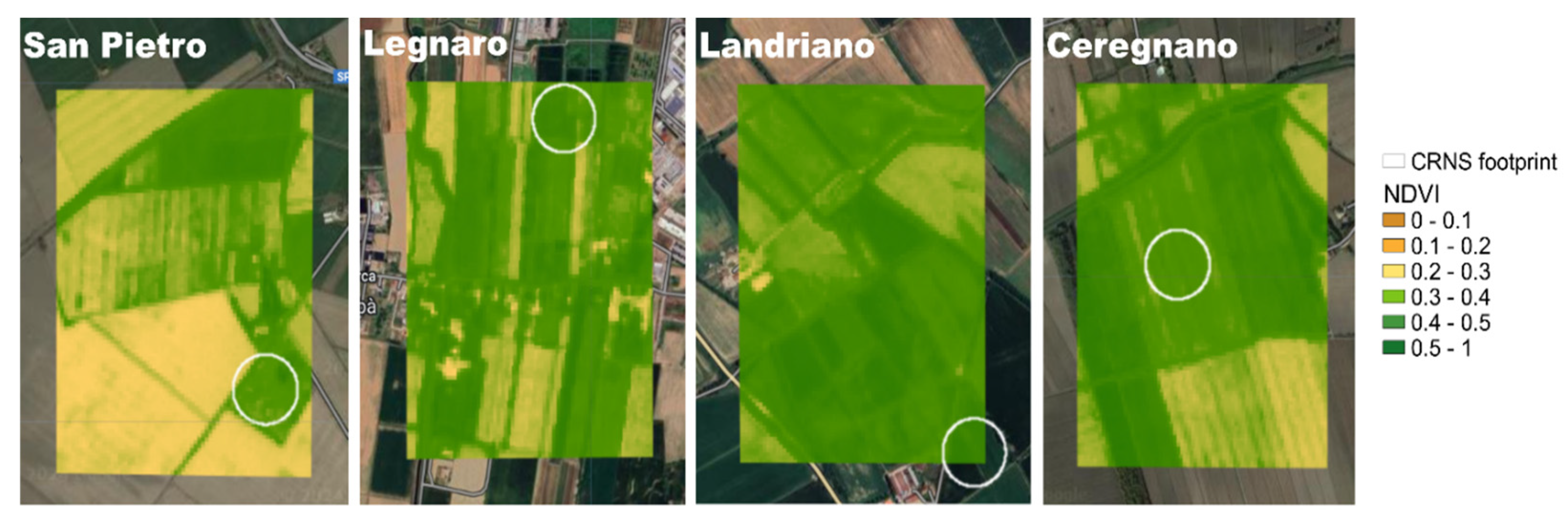
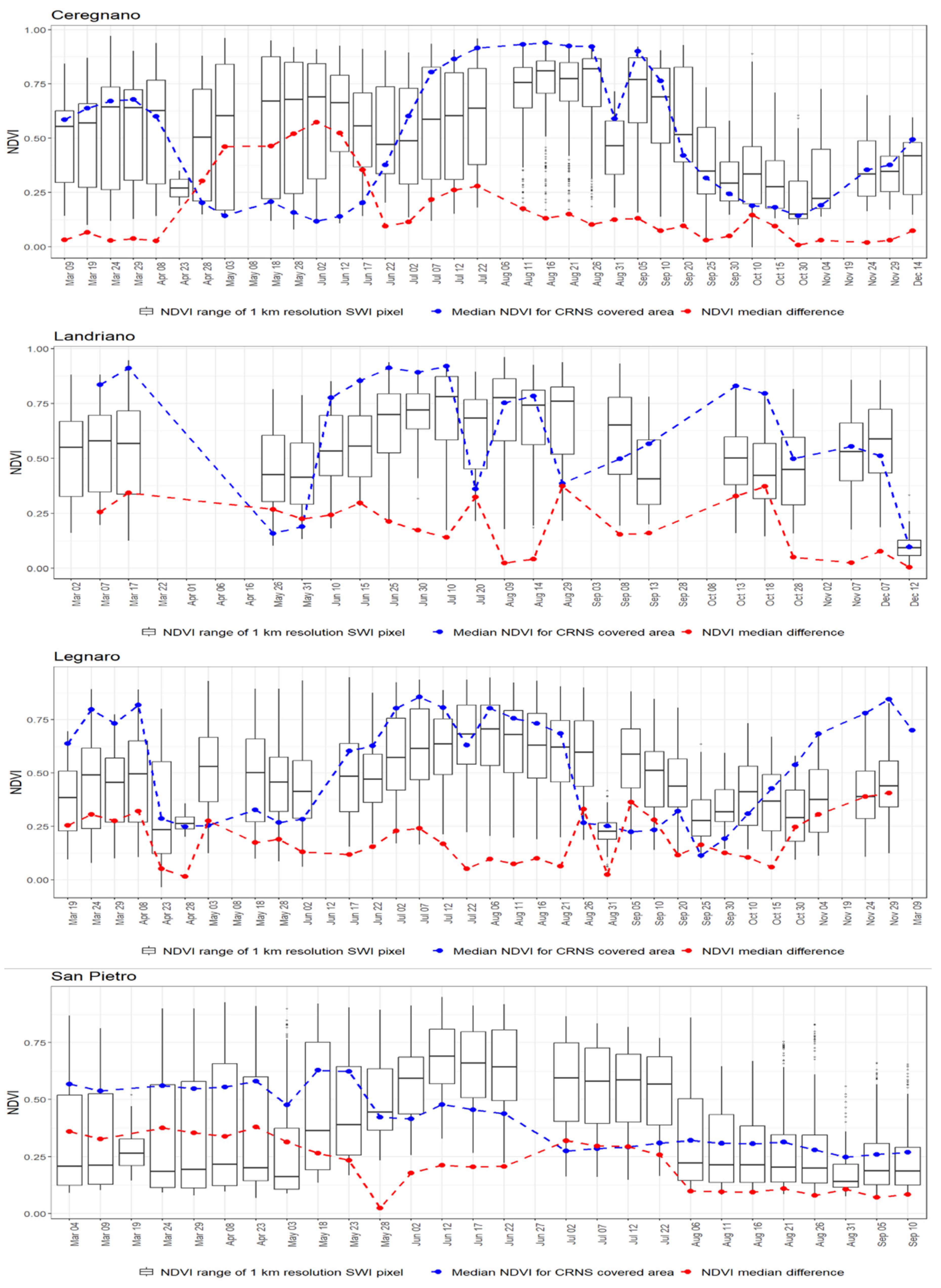
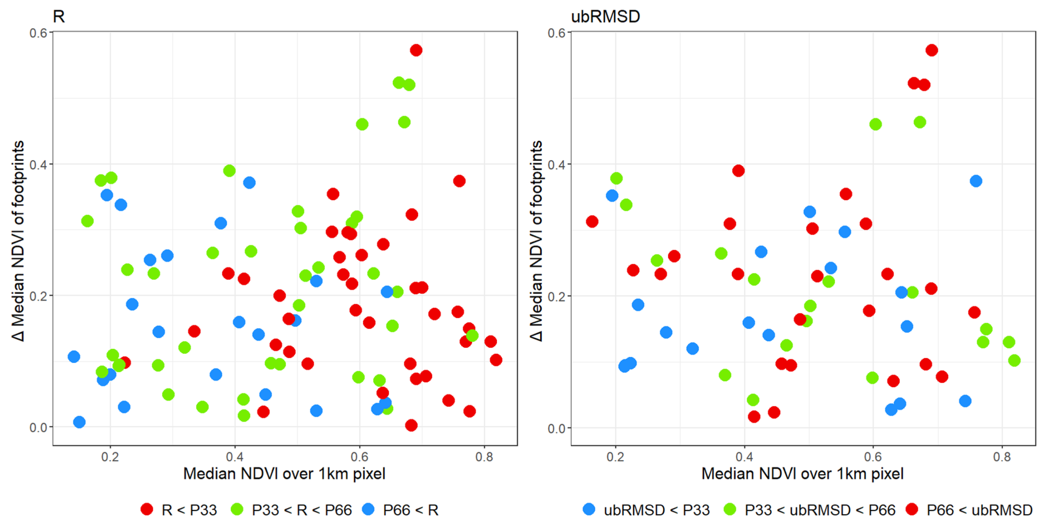
3.2.1. SWC Variability as a Function of Vegetation

Figure 4 and Figure 5 provide spatial and temporal overviews of the NDVI variations over the areas covered by CRNS and the RS pixel, respectively. Specifically, Figure 4 shows the median NDVI values over the study period for each of the four sites. In contrast, Figure 5 shows how the spatial variability (boxplot) changes over time. Medians NDVI and differences between the medians NDVI over the pixel and over the CRNS footprint are also plotted.

Generally, we notice a relatively high spatial variability of the NDVI over the RS pixel (Figure 5, boxplot). However, the difference between the median NDVI over the pixel and over the CRNS footprint is low (<0.25), suggesting good representativeness of the CRNS location for RS comparison. The highest absolute difference in the medians of NDVI values occurs in Ceregnano, reaching 0.57 in May. Noteworthily, this site had the lowest performance when comparing SWC products.

To further investigate this effect, Figure 6 provides a more detailed examination of the relationship between greenness and the performance of SWC products. For two statistics, and by aggregating data from all sites, the y-axis illustrates the difference in the median of NDVI of the footprints, while the x-axis represents the median NDVI over RS pixels. In this scatterplot, the color of points indicates three separate classes for each metric. These classes were chosen based on the 33rd and 66th percentiles (P33 and P66) of their datasets, with blue representing P66 < R in the left panel (T = 2) and ubRMSD < P33 in the right panel (T = 2), indicating stronger scores. The scattering of red points for R suggests that weaker scores occur when the NDVI of the pixel has higher values, while the dispersion of points for ubRMSD suggests that vegetation does not affect the performance in the absolute differences. However, for both R and ubRMSD, it can be observed that high scores are not present when there is a high difference in NDVI (i.e., >0.4).

To conduct a more quantitative analysis, we compared seasonal ubRMSD (e.g., Figure 3, right panel) with absolute differences in the median NDVI of footprints (Figure 5, red lines). To align the sample lengths, piecewise linear interpolation was applied to the absolute differences in median NDVI, ensuring a consistent temporal resolution between the time series. We then used R to measure the correlation between these two series (

Table 3. Correlation R between NDVI differences and seasonal ubRMSD at the four experimental sites for different T values.

Site	T-Values	R
Ceregnano	T = 2	0.48
	T = 5	0.50
	T = 10	0.58 1
Landriano	T = 2	−0.38
	T = 5	0.10
	T = 10	0.13
Legnaro	T = 2	−0.03
	T = 5	0.31
	T = 10	0.32
San Pietro	T = 2	0.13
	T = 5	0.12
	T = 10	0.38
All sites (mean)	T = 2	0.05
	T = 5	0.26
	T = 10	0.35 2

¹ The highest R among sites. ² The mean R of all sites for T = 10.

). The analysis shows a positive correlation (R) across all sites when T value = 5 and T value = 10 are considered. The mean R for all sites (T = 10) is 0.35; the highest correlation is for Ceregnano (R = 0.58) and the lowest for Landriano (R = 0.13). This result confirms that the higher the differences between the NDVI, the lower the agreement between the SWI products. Noteworthily, when T-value = 2 is considered, the results at two sites still show a positive correlation (San Pietro and Legnaro), while two sites show a negative correlation (Landriano and Ceregnano). This difference can be explained considering that SWC variability at deeper soil layers (i.e., T > 2) could be more affected by vegetation while the SWC dynamic at a shallow soil depth (i.e., T = 2) could be more affected by the atmospheric conditions (e.g., precipitation and air temperature) [58,59].

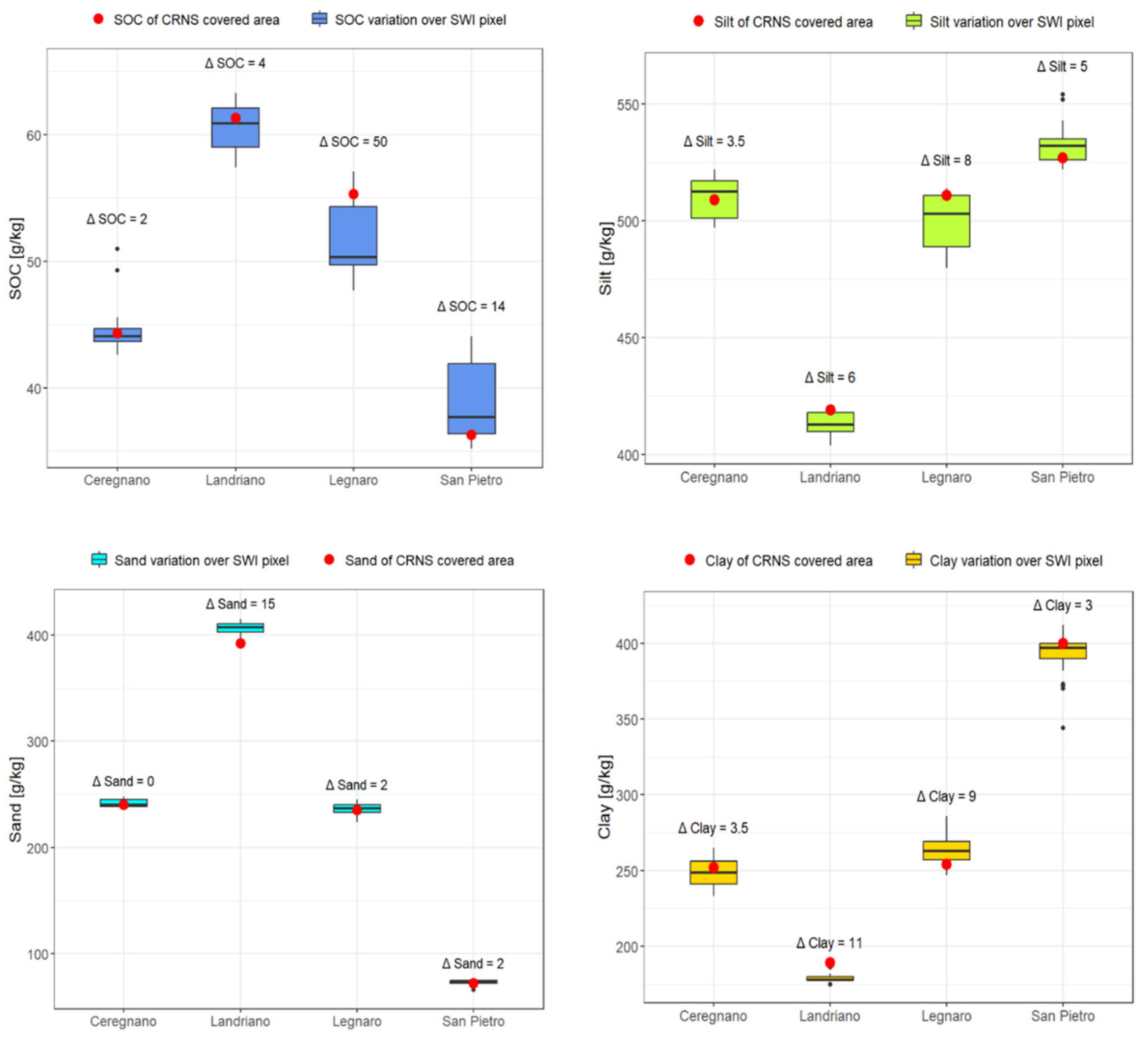
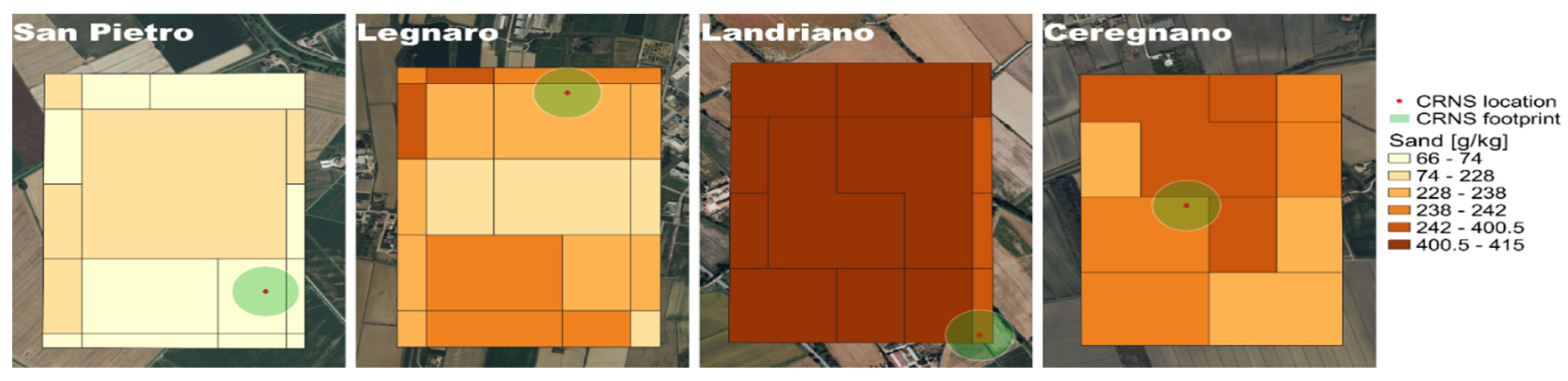
3.2.2. Soil Effect on SWC Mismatch

Referring to soil characteristics, Figure 7 illustrates soil heterogeneity by comparing the variation in soil texture components and SOC around the median value within RS pixels (depicted as the black line inside colored box plots) and their corresponding values for CRNS footprints (highlighted as red points) across four sites. Figure 8 shows the spatial variability of g/kg of sand at the four sites, as an example.

Taking all properties into account, Legnaro exhibits the greatest difference in medians, trailed by Landriano, San Pietro, and Ceregnano, respectively. However, these differences do not relate to the performance ranking (see Table 2). For this reason, the results suggest that the difference between the median properties over the RS pixel and the soil in the CRNS footprint is not relevant. Some more insight can be seen by looking at spatial variability and soil type. Specifically, Landriano, where we had the best agreement between the SWC products, has loam soil (with a high percentage of sand and SOC in comparison to other sites) and a relatively low spatial variability within the RS pixel. In contrast, the other sites that showed lower performance have higher percentages of silt and clay (>500 g/kg and 250 g/kg, respectively) and higher spatial variability. Despite the fact that the information provided by SoilGrids should be taken with caution due to inherent uncertainty at this scale, the results suggest how the soil spatial variability and the soil type could be relevant factors in explaining the different agreements in the SWC products.

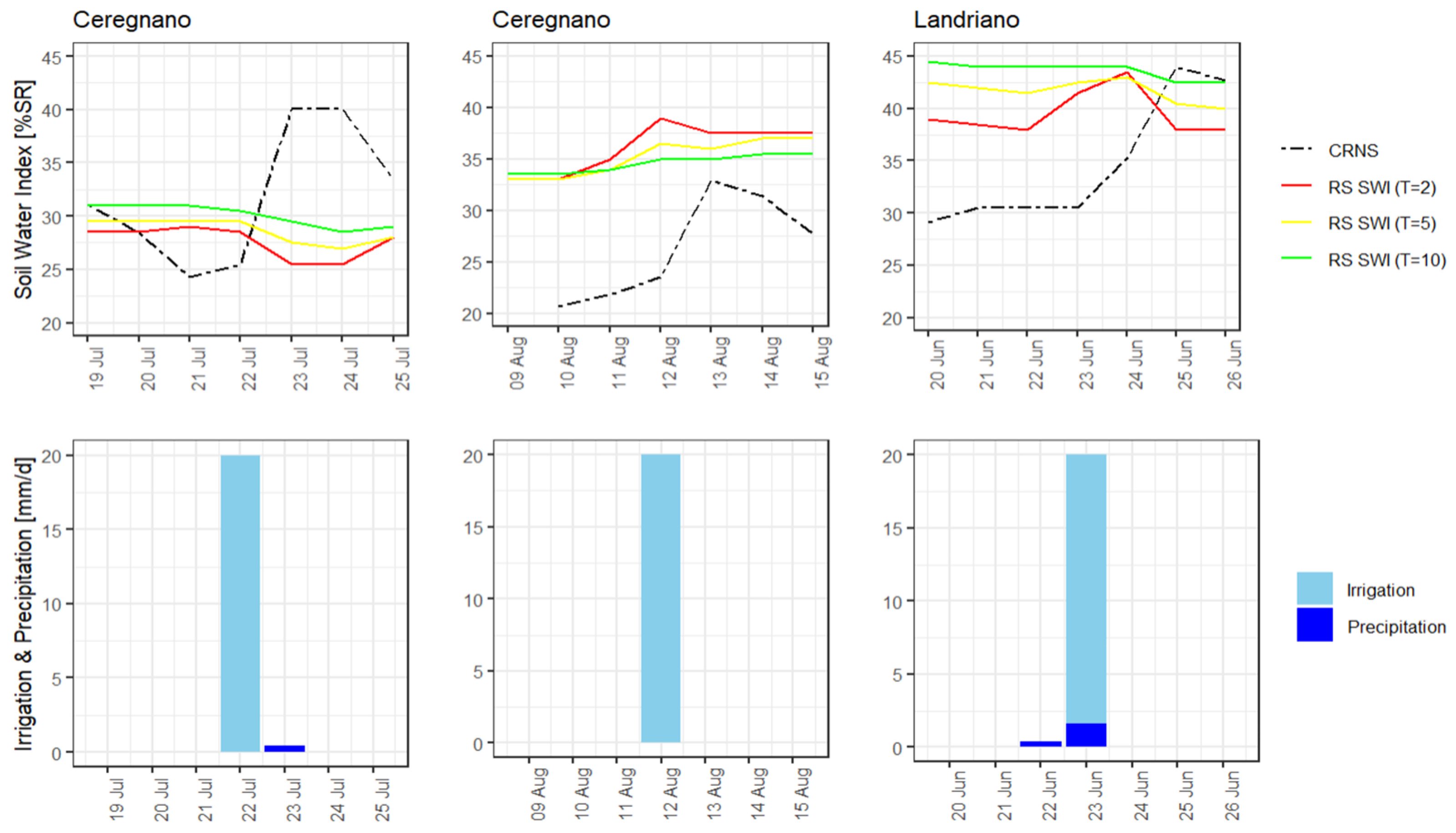
3.2.3. Deviations in SWC in Relation to the Irrigation Management

Figure 9 shows the noticeable effect of irrigation on the CRNS values of both sites, resulting in an increase of more than 10%SR. A potential effect of irrigation on RS at T = 2 is notable at Landriano and Ceregnano (only for the irrigation event of 12 August), but the signal increases earlier and to a lesser extent (i.e., around 5%SR). While these results suggest that the RS product, unlike CRNS, is less sensitive to the irrigation events, it should be noted that the irrigation events recorded at the CRNS footprint could also not well represent the RS resolution. Neighboring fields could have not been irrigated at Ceregnano, smoothing the effect of the irrigation of the CRNS area over the RS pixel. In contrast, neighboring fields could have been irrigated earlier at Landriano, explaining the early increase of RS-derived SWI. For this reason, this comparison underlines the need for irrigation information over the entire pixel for a proper assessment of RS soil moisture products and the capability to assess irrigation amount properly [60].

4. Discussion

The strong correlation between precipitation and SWC observations shows the sensitivity of the measurements to external factors. The higher agreement between CRNS data and TDR observations confirms the accuracy of the former in quantifying SWC and suggests that CRNS could serve as a valuable assessment reference. RS-derived SWI (T = 2) showing greater fluctuation and dynamic alignment with CRNS aligns with the expectation that both products primarily capture SWC from upper soil layers. Increasing depth brings enhanced stability to the observed trend, and naturally, this also influences the overall decrease in the SWI quantity. Therefore, it can be concluded that considering that CRNS and RS are more sensitive to upper layers, consistent with previous studies [37], the best T for our studied areas in the case of evaluating SCARSAR-SWI data is T = 2. The R reinforces this observation, indicating that the shallower depth (T = 2) provides a better match to CRNS data. The slight decrease in ubRMSD with increasing depth can be explained by the enhanced stability in trends for deeper layers and the fact that ubRMSD reflects the overall agreement in means.

The observed metrics of the raw SWI time series align with the site characteristics presented in Figure 1 and Figure 4. Landriano, with high homogeneity of vegetation greenness, exhibits the strongest match, while Ceregnano and San Pietro, with dividable parts inside their satellite pixels, show weaker results. San Pietro shows even stronger different behavior than other sites, it experiences a considerable mismatch of SWC products between June and October, attributed to the grass-covered CRNS area surrounded by dense maize fields; this grass-covered area becomes notably dry in the summer period.

The examination of the 35-day performance metrics provided valuable insights into the CRNS and RS-derived SWI relationship, emphasizing the significance of considering seasonality when assessing SWC dynamics. This approach highlighted improved statistics in smaller time intervals, reinforcing the importance of detailed analyses. Lower metrics during the summer period (drop of R in August to around zero) are attributed to various factors, including varying biomass growth rates among crops (which is also obvious in Figure 4), diverse irrigation practices, and differing harvesting schedules across fields. The slight decrease in metrics during the winter period and observed SCATSAR-SWI overestimation need further studies, including on-site field investigation in the last months of the year. Among other factors already highlighted in previous studies, like vegetation and soil roughness [61], the presence of dew and fog in agricultural fields of northern Italy during the winter should be considered [62]. Dew and fog significantly impact the signals from remote sensing, particularly microwave remote sensing, by affecting leaf surface wetness and potentially altering soil moisture estimations. The presence of surface water generally increases the signal detected but it can complicate accurate soil moisture measurement [63].

One critical aspect that warrants deeper exploration is the potential source of uncertainty introduced through the fusion of data from different active remote sensing platforms, such as Sentinel-1 and ASCAT. While both sensors operate at the same radar frequency (C-band), their key difference lies in their spatial resolution. Sentinel-1, with its higher spatial resolution, can capture more detailed surface-level variations [64], whereas ASCAT, with its coarser resolution, integrates signals over a larger area. This difference in spatial resolution could lead to discrepancies in the observed SWC, particularly in heterogeneous landscapes where soil properties and moisture conditions vary significantly over short distances. The fusion process must account for these differences in resolution to avoid inconsistencies in SWC measurements.

Moving to spatial mismatch investigations, better alignment of RS-derived SWI (T = 10) with NDVI variations could be explained by the lag in the impact of SWC on vegetation growth, where stability in SWI (T = 10) better reflects the overall conditions over time, considering the time required for the water to infiltrate deeper soil layers.

Despite the generally weak results of R when comparing seasonal ubRMSD of SWC products and the absolute difference of median NDVI of two footprints (Table 3), the outcomes reveal that the ranking, in this case, is completely revered considering the grading of R we had when comparing SWC products. Notably, Ceregnano shows a higher correlation in this analysis, while Landriano exhibits a lower correlation. This shift in rankings suggests that, in cases with higher disparities in SWC products, the discrepancy tends to be more related to alterations in NDVI within different footprints. Therefore, although the difference in the vegetation vigor of footprints cannot be introduced as a crucial agent for spatial representativeness, it is one of the factors that shows its effect.

Figure 6 illustrates the correlation of NDVI heterogeneity and median NDVI of the 1 km pixel with performance scores among SWC products. The behavior of R classes, where lower correlation tends to be more present on the right side of the plot where the median NDVI of RS pixels is high, supports the notion that biomass growth leads to weaker correlations of SWC products. Additionally, the absence of higher scores of both R and ubRMSD in areas with large differences in NDVI demonstrates the slight impact of NDVI heterogeneity between footprints on lower scores of SWC product matches.

Regarding soil properties, the rank of sites based on their soil homogeneity between footprints differs from the initial results of metrics between SWC products. This outcome for our studied areas prevents us from concluding that the difference in soil texture elements (sand, clay, and silt) and SOC between footprints is representative of a spatial mismatch between areas covered by CRNS and RS. However, sites with less variation in the RS pixel tended to perform better when comparing SWC products (see Figure 7 and Figure 8), which indicates that soil properties play a notable role in explaining the differences in performance scores between CRNS and RS. Variability in soil texture and SOC levels within RS pixels affects the accuracy of SWC products. It is worth noting that sites with a lower percentage of sand and SOC (silt loam soil type) generally had lower performance metrics compared to sites with a loam soil type, such as Landriano, when evaluating SWC products.

The disparity in responses between CRNS records and RS-derived SWC to irrigation events in Ceregnano and Landriano (Figure 9) underscores CRNS’s heightened sensitivity to localized perturbations, likely owing to its finer spatial resolution enabling it to capture localized changes more effectively within its footprint. Conversely, RS products, with their larger pixel size, may attenuate their ability to distinguish irrigation effects. Essentially, for this matter, we also require information about irrigation amount and date in neighboring areas within the RS pixels. This underscores the significance of irrigation practices as a factor influencing spatial variability and representativeness. Having a comprehensive understanding of irrigation is crucial for comparing soil moisture data from various sources and scales effectively. Nonetheless, the detection of irrigation impact by RS-derived SWC, notably at depth T = 2 in Landriano and Ceregnano (only the irrigation event of 12 August), adds credit to the efficacy of this method in agricultural monitoring.

The remote sensing component of this study requires further elaboration. The fusion of ASCAT and Sentinel-1 data to produce a high-resolution SWC product is a significant advancement, but it comes with inherent limitations. The SCATSAR-SWI product does not account for soil texture in its retrieval process, which can lead to inaccuracies in representing soil depths, particularly in heterogeneous agricultural fields. This limitation is evident in the observed differences between SWC estimates at sites with varied soil textures and land use practices. The influence of Soil Organic Carbon and sand content on the RS-derived SWC also warrants closer examination, as these factors were found to correlate to decreased agreement between the SWC products. By integrating soil texture data into the RS product’s retrieval algorithm, future research could enhance the accuracy of SWC estimates, thereby improving the utility of RS in precision agriculture.

Overall, this study highlights the need for an ongoing understanding of the complex interplay of the different factors like vegetation, soil properties, and irrigation practices for a proper intercomparison of the SWC products. These would put the basis for identifying the best representative location or for developing and integrating upscaling and downscaling techniques that should applied to harmonize the spatial mismatch.

5. Conclusions

This study compares the SCATSAR-SWI, a combined RS product for daily SWC at different depths (T-values) at a kilometer scale, to Cosmic Ray Neutron Sensing (CRNS) across four agricultural sites in northern Italy. Spatial variability and representativeness are explored by means of the Normalized Difference Vegetation Index (NDVI), soil properties (soil texture and Soil Organic Carbon), and irrigation practices. The analysis revealed notable insights into the dynamics and accuracy of SWC estimation, as well as the influence of spatial heterogeneity on comparison outcomes.

Higher agreement between CRNS data and Time Domain Reflectometry (TDR) points (additional measurements for improved investigation) suggests that CRNS can serve as a valuable assessment reference, demonstrating its merit in capturing the dynamics of SWC to a good extent. RS-derived SWI showcased reasonable compliance with CRNS for all sites. SCATSAR-SWI (T = 2) exhibited the best alignment among T-values, with the mean Pearson correlation coefficient (R) of 0.6 and unbiased Root–Mean–Square Difference (ubRMSD) of 14.90%SR, suggesting the shallow depth as being optimal for evaluating SCATSAR-SWI in the studied areas.

Seasonal variations in performance metrics highlighted the importance of considering seasonality in assessing SWC dynamics, with lower metrics observed during the summer period interpreted by high biomass growth and irrigation practices. Further examination is required to understand the slight decline in metrics during the winter season and the observed overestimation in SCATSAR-SWI. Among other factors, in this study, the presence of intense leaf wetness and its subsequent impact on the increase of the SAR signal could explain the behavior, and it should be further explored.

Moving to investigations of spatial inconsistencies, the improved alignment between SWI (T = 10) and variations in NDVI is attributed to the delay in the influence of SWC on vegetation growth. In this context, the stability observed in SWI (T = 10) better reflects the overall conditions over time. Analyses indicate that as NDVI values and their variation within RS pixels increase, the correlation between SWC products diminishes. Despite generally weak scores (mean R of 0.35), when analyzing the impact of NDVI differences on the performance metric between SWC products, the findings suggest that in instances with greater disparities in SWC products, the variation tends to be more closely associated with changes in NDVI across different footprints. Thus, while the difference in vegetation vigor of footprints cannot be singled out as the sole determinant for spatial representativeness, it does demonstrate an influential factor.

Examining SoilGrids’ soil property maps, considering the fact that the information provided by this platform should be taken with caution due to inherent uncertainty, reveals that the ranking of sites according to their soil uniformity between footprints differs from the initial findings regarding metrics among SWC products. Therefore, this aspect in our sites cannot be considered an aiding element in the matter of understanding spatial representativeness. On the other hand, investigating the variation of soil properties within the RS pixel shows that sites with less variation had better rank when comparing SWC products, which indicates variability in soil texture and SOC levels within the RS pixel affects the accuracy of SWC products. It is noteworthy that locations with silt loam soil type typically exhibited inferior performance metrics in comparison to sites with loam soil type when assessing SWC products.

Considering irrigation, the impact of these events on SWC levels was more pronounced in CRNS measurements compared to RS. This difference highlights the need for information on irrigation in neighboring areas within RS pixels to properly assess soil moisture products. These studies highlight the importance of considering irrigation as a factor affecting spatial variability and representativeness, emphasizing the importance of comprehensive irrigation information gathering within RS pixels. Despite RS products showing less sensitivity to irrigation events, their ability to detect irrigation impacts adds credibility to their effectiveness in agricultural monitoring.

Overall, the results highlight how RS pixel variability of the different environmental factors can explain differences between SWC products. Based on this present study, it is recommended for RS-derived SWC product assessment to dim the influence of summer and winter seasons and to select pixels with the lowest variability of vegetation greenness (NDVI), soil properties (sand, silt, clay, and SOC), and irrigation management. Alternatively, protocols to identify the location of ground observations more representative of the RS pixel should be tested and implemented.

References

1. Engman, E.T. Applications of Microwave Remote Sensing of Soil Moisture for Water Resources and Agriculture. Remote Sens. Environ. 1991, 35, 213–226. [Google Scholar] [CrossRef]
2. Wagner, W.; Lemoine, G.; Rott, H. A Method for Estimating Soil Moisture from ERS Scatterometer and Soil Data. Remote Sens. Environ. 1999, 70, 191–207. [Google Scholar] [CrossRef]
3. Arias, M.; Notarnicola, C.; Campo-Bescós, M.Á.; Arregui, L.M.; Álvarez-Mozos, J. Evaluation of Soil Moisture Estimation Techniques Based on Sentinel-1 Observations over Wheat Fields. Agric. Water Manag. 2023, 287, 108422. [Google Scholar] [CrossRef]
4. Mälicke, M.; Hassler, S.K.; Blume, T.; Weiler, M.; Zehe, E. Soil Moisture: Variable in Space but Redundant in Time. Hydrol. Earth Syst. Sci. 2020, 24, 2633–2653. [Google Scholar] [CrossRef]
5. Haghighi, E.; Short Gianotti, D.J.; Akbar, R.; Salvucci, G.D.; Entekhabi, D. Soil and Atmospheric Controls on the Land Surface Energy Balance: A Generalized Framework for Distinguishing Moisture-Limited and Energy-Limited Evaporation Regimes. Water Resour. Res. 2018, 54, 1831–1851. [Google Scholar] [CrossRef]
6. Domínguez-niño, J.M.; Oliver-manera, J.; Arbat, G.; Girona, J.; Casadesús, J. Analysis of the Variability in Soil Moisture Measurements by Capacitance Sensors in a Drip-Irrigated Orchard. Sensors 2020, 20, 5100. [Google Scholar] [CrossRef]
7. Babaeian, E.; Sadeghi, M.; Jones, S.B.; Montzka, C.; Vereecken, H.; Tuller, M. Ground, Proximal, and Satellite Remote Sensing of Soil Moisture. Rev. Geophys. 2019, 57, 530–616. [Google Scholar] [CrossRef]
8. Kovanič, L.; Blistan, P.; Urban, R.; Štroner, M.; Blišt’anová, M.; Bartoš, K.; Pukanská, K. Analysis of the Suitability of High-Resolution DEM Obtained Using ALS and UAS (SfM) for the Identification of Changes and Monitoring the Development of Selected Geohazards in the Alpine Environment—A Case Study in High Tatras, Slovakia. Remote Sens. 2020, 12, 3901. [Google Scholar] [CrossRef]
9. Loew, A.; Bell, W.; Brocca, L.; Bulgin, C.E.; Burdanowitz, J.; Calbet, X.; Donner, R.V.; Ghent, D.; Gruber, A.; Kaminski, T.; et al. Validation Practices for Satellite-Based Earth Observation Data across Communities. Rev. Geophys. 2017, 55, 779–817. [Google Scholar] [CrossRef]
10. Gruber, A.; De Lannoy, G.; Albergel, C.; Al-Yaari, A.; Brocca, L.; Calvet, J.C.; Colliander, A.; Cosh, M.; Crow, W.; Dorigo, W.; et al. Validation Practices for Satellite Soil Moisture Retrievals: What Are (the) Errors? Remote Sens. Environ. 2020, 244, 111806. [Google Scholar] [CrossRef]
11. Dorigo, W.A.; Gruber, A.; De Jeu, R.A.M.; Wagner, W.; Stacke, T.; Loew, A.; Albergel, C.; Brocca, L.; Chung, D.; Parinussa, R.M.; et al. Evaluation of the ESA CCI Soil Moisture Product Using Ground-Based Observations. Remote Sens. Environ. 2015, 162, 380–395. [Google Scholar] [CrossRef]
12. Dorigo, W.A.; Wagner, W.; Hohensinn, R.; Hahn, S.; Paulik, C.; Xaver, A.; Gruber, A.; Drusch, M.; Mecklenburg, S.; Van Oevelen, P.; et al. The International Soil Moisture Network: A Data Hosting Facility for Global in Situ Soil Moisture Measurements. Hydrol. Earth Syst. Sci. 2011, 15, 1675–1698. [Google Scholar] [CrossRef]
13. Brocca, L.; Morbidelli, R.; Melone, F.; Moramarco, T. Soil Moisture Spatial Variability in Experimental Areas of Central Italy. J. Hydrol. 2007, 333, 356–373. [Google Scholar] [CrossRef]
14. Bogena, H.R.; Huisman, J.A.; Güntner, A.; Hübner, C.; Kusche, J.; Jonard, F.; Vey, S.; Vereecken, H. Emerging Methods for Noninvasive Sensing of Soil Moisture Dynamics from Field to Catchment Scale: A Review. Wiley Interdiscip. Rev. Water 2015, 2, 635–647. [Google Scholar] [CrossRef]
15. Ochsner, T.E.; Cosh, M.H.; Cuenca, R.H.; Dorigo, W.A.; Draper, C.S.; Hagimoto, Y.; Kerr, Y.H.; Larson, K.M.; Njoku, E.G.; Small, E.E.; et al. State of the Art in Large-Scale Soil Moisture Monitoring. Soil Sci. Soc. Am. J. 2013, 77, 1888–1919. [Google Scholar] [CrossRef]
16. Zreda, M.; Desilets, D.; Ferré, T.P.A.; Scott, R.L. Measuring Soil Moisture Content Non-Invasively at Intermediate Spatial Scale Using Cosmic-Ray Neutrons. Geophys. Res. Lett. 2008, 35. [Google Scholar] [CrossRef]
17. Zhu, X.; Shao, M.; Zeng, C.; Jia, X.; Huang, L.; Zhang, Y.; Zhu, J.; Zhu, X.; Shao, M.; Zeng, C.; et al. Application of Cosmic-Ray Neutron Sensing to Monitor Soil Water Content in an Alpine Meadow Ecosystem on the Northern Tibetan Plateau. J. Hydrol. 2016, 536, 247–254. [Google Scholar] [CrossRef]
18. Baatz, R.; Bogena, H.R.; Hendricks Franssen, H.J.; Huisman, J.A.; Montzka, C.; Vereecken, H. An Empirical Vegetation Correction for Soil Water Content Quantification Using Cosmic Ray Probes. Water Resour. Res. 2015, 51, 2030–2046. [Google Scholar] [CrossRef]
19. Baroni, G.; Scheiffele, L.M.; Schrön, M.; Ingwersen, J.; Oswald, S.E. Uncertainty, Sensitivity and Improvements in Soil Moisture Estimation with Cosmic-Ray Neutron Sensing. J. Hydrol. 2018, 564, 873–887. [Google Scholar] [CrossRef]
20. Gianessi, S.; Polo, M.; Stevanato, L.; Lunardon, M.; Francke, T.; Oswald, S.E.; Said Ahmed, H.; Toloza, A.; Weltin, G.; Dercon, G.; et al. Testing a Novel Sensor Design to Jointly Measure Cosmic-Ray Neutrons, Muons and Gamma Rays for Non-Invasive Soil Moisture Estimation. Geosci. Instrum. Methods Data Syst. 2024, 13, 9–25. [Google Scholar] [CrossRef]
21. Baroni, G.; Oswald, S.E. A Scaling Approach for the Assessment of Biomass Changes and Rainfall Interception Using Cosmic-Ray Neutron Sensing. J. Hydrol. 2015, 525, 264–276. [Google Scholar] [CrossRef]
22. A, Y.; Wang, G.; Hu, P.; Lai, X.; Xue, B.; Fang, Q. Root-Zone Soil Moisture Estimation Based on Remote Sensing Data and Deep Learning. Environ. Res. 2022, 212, 113278. [Google Scholar] [CrossRef]
23. Babaeian, E.; Sadeghi, M.; Franz, T.E.; Jones, S.; Tuller, M. Mapping Soil Moisture with the OPtical TRApezoid Model (OPTRAM) Based on Long-Term MODIS Observations. Remote Sens. Environ. 2018, 211, 425–440. [Google Scholar] [CrossRef]
24. Mengen, D.; Jagdhuber, T.; Balenzano, A.; Mattia, F.; Vereecken, H.; Montzka, C. High Spatial and Temporal Soil Moisture Retrieval in Agricultural Areas Using Multi-Orbit and Vegetation Adapted Sentinel-1 SAR Time Series. Remote Sens. 2023, 15, 2282. [Google Scholar] [CrossRef]
25. Beale, J.; Waine, T.; Evans, J.; Corstanje, R. A Method to Assess the Performance of SAR-Derived Surface Soil Moisture Products. IEEE J. Sel. Top. Appl. Earth Obs. Remote Sens. 2021, 14, 4504–4516. [Google Scholar] [CrossRef]
26. Balenzano, A.; Satalino, G.; Lovergine, F.; Rinaldi, M.; Iacobellis, V.; Mastronardi, N.; Mattia, F. On the Use of Temporal Series of L- and X-Band SAR Data for Soil Moisture Retrieval. Capitanata Plain Case Study. Eur. J. Remote Sens. 2013, 46, 721–737. [Google Scholar] [CrossRef]
27. Balenzano, A.; Mattia, F.; Satalino, G.; Davidson, M.W.J. Dense Temporal Series of C- and L-Band SAR Data for Soil Moisture Retrieval Over Agricultural Crops. IEEE J. Sel. Top. Appl. Earth Obs. Remote Sens. 2011, 4, 439–450. [Google Scholar] [CrossRef]
28. Wagner, W.; Hahn, S.; Kidd, R.; Melzer, T.; Bartalis, Z.; Hasenauer, S.; Figa-Saldaña, J.; De Rosnay, P.; Jann, A.; Schneider, S.; et al. The ASCAT Soil Moisture Product: A Review of Its Specifications, Validation Results, and Emerging Applications. Meteorol. Z. 2013, 22, 5–33. [Google Scholar] [CrossRef]
29. Mohanty, B.P.; Cosh, M.H.; Lakshmi, V.; Montzka, C. Soil Moisture Remote Sensing: State-of-the-Science. Vadose Zone J. 2017, 16, 1–9. [Google Scholar] [CrossRef]
30. Bauer-Marschallinger, B.; Freeman, V.; Cao, S.; Paulik, C.; Schaufler, S.; Stachl, T.; Modanesi, S.; Massari, C.; Ciabatta, L.; Brocca, L.; et al. Toward Global Soil Moisture Monitoring With Sentinel-1: Harnessing Assets and Overcoming Obstacles. IEEE Trans. Geosci. Remote Sens. 2019, 57, 520–539. [Google Scholar] [CrossRef]
31. Bauer-Marschallinger, B.; Paulik, C.; Hochstöger, S.; Mistelbauer, T.; Modanesi, S.; Ciabatta, L.; Massari, C.; Brocca, L.; Wagner, W. Soil Moisture from Fusion of Scatterometer and SAR: Closing the Scale Gap with Temporal Filtering. Remote Sens. 2018, 10, 1030. [Google Scholar] [CrossRef]
32. Chen, T.; de Jeu, R.A.M.; Liu, Y.Y.; van der Werf, G.R.; Dolman, A.J. Using Satellite Based Soil Moisture to Quantify the Water Driven Variability in NDVI: A Case Study over Mainland Australia. Remote Sens Environ. 2014, 140, 330–338. [Google Scholar] [CrossRef]
33. Farrar, T.J.; Nicholson, S.E.; Lare, A.R. The Influence of Soil Type on the Relationships between NDVI, Rainfall, and Soil Moisture in Semiarid Botswana. II. NDVI Response to Soil Oisture. Remote Sens. Environ. 1994, 50, 121–133. [Google Scholar] [CrossRef]
34. Martínez-Fernández, J.; González-Zamora, A.; Almendra-Martín, L. Soil Moisture Memory and Soil Properties: An Analysis with the Stored Precipitation Fraction. J. Hydrol. 2021, 593, 125622. [Google Scholar] [CrossRef]
35. Schrön, M.; Köhli, M.; Scheiffele, L.; Iwema, J.; Bogena, H.R.; Lv, L.; Martini, E.; Baroni, G.; Rosolem, R.; Weimar, J.; et al. Improving Calibration and Validation of Cosmic-Ray Neutron Sensors in the Light of Spatial Sensitivity. Hydrol. Earth Syst. Sci. 2017, 21, 5009–5030. [Google Scholar] [CrossRef]
36. Franz, T.E.; Zreda, M.; Rosolem, R.; Ferre, T.P.A. Field Validation of a Cosmic-Ray Neutron Sensor Using a Distributed Sensor Network. Vadose Zone J. 2012, 11. [Google Scholar] [CrossRef]
37. Montzka, C.; Bogena, H.R.; Zreda, M.; Monerris, A.; Morrison, R.; Muddu, S.; Vereecken, H. Validation of Spaceborne and Modelled Surface Soil Moisture Products with Cosmic-Ray Neutron Probes. Remote Sens. 2017, 9, 103. [Google Scholar] [CrossRef]
38. Saxton, K.E.; Rawls, W.J. Soil Water Characteristic Estimates by Texture and Organic Matter for Hydrologic Solutions. Soil Sci. Soc. Am. J. 2006, 70, 1569–1578. [Google Scholar] [CrossRef]
39. van Genuchten, M.T. A Closed-form Equation for Predicting the Hydraulic Conductivity of Unsaturated Soils. Soil Sci. Soc. Am. J. 1980, 44, 892–898. [Google Scholar] [CrossRef]
40. Topp, G.C.; Davis, J.L.; Annan, A.P. Electromagnetic Determination of Soil Water Content Using TDR: I. Applications to Wetting Fronts and Steep Gradients. Soil Sci. Soc. Am. J. 1982, 46, 672–678. [Google Scholar] [CrossRef]
41. Topp, G.C.; Davis, J.L.; Bailey, W.G.; Zebchuk, W.D. The Measurement of Soil Water Content Using a Portable TDR Hand Probe. Can. J. Soil Sci. 1984, 64, 313–321. [Google Scholar] [CrossRef]
42. Madelon, R.; Rodríguez-Fernández, N.J.; Bazzi, H.; Baghdadi, N.; Albergel, C.; Dorigo, W.; Zribi, M. Soil Moisture Estimates at 1 Km Resolution Making a Synergistic Use of Sentinel Data. Hydrol. Earth Syst. Sci. 2023, 27, 1221–1242. [Google Scholar] [CrossRef]
43. Balenzano, A.; Mattia, F.; Satalino, G.; Lovergine, F.P.; Palmisano, D.; Davidson, M.W.J. Dataset of Sentinel-1 Surface Soil Moisture Time Series at 1 Km Resolution over Southern Italy. Data Brief 2021, 38, 107345. [Google Scholar] [CrossRef] [PubMed]
44. Peng, J.; Albergel, C.; Balenzano, A.; Brocca, L.; Cartus, O.; Cosh, M.H.; Crow, W.T.; Dabrowska-Zielinska, K.; Dadson, S.; Davidson, M.W.J.; et al. A Roadmap for High-Resolution Satellite Soil Moisture Applications—Confronting Product Characteristics with User Requirements. Remote Sens. Environ. 2021, 252, 112162. [Google Scholar] [CrossRef]
45. De Lange, R.; Beck, R.; Van De Giesen, N.; Friesen, J.; De Wit, A.; Wagner, W. Scatterometer-Derived Soil Moisture Calibrated for Soil Texture with a One-Dimensional Water-Flow Model. IEEE Trans. Geosci. Remote Sens. 2008, 46, 4041–4049. [Google Scholar] [CrossRef]
46. Crow, W.T.; Berg, A.A.; Cosh, M.H.; Loew, A.; Mohanty, B.P.; Panciera, R.; De Rosnay, P.; Ryu, D.; Walker, J.P. Upscaling Sparse Ground-Based Soil Moisture Observations for the Validation of Coarse-Resolution Satellite Soil Moisture Products. Rev. Geophys. 2012, 50. [Google Scholar] [CrossRef]
47. Zhang, H.; Chang, J.; Zhang, L.; Wang, Y.; Li, Y.; Wang, X. NDVI Dynamic Changes and Their Relationship with Meteorological Factors and Soil Moisture. Environ. Earth Sci. 2018, 77, 582. [Google Scholar] [CrossRef]
48. Wang, G.; Zhang, X.; Yinglan, A.; Duan, L.; Xue, B.; Liu, T. A Spatio-Temporal Cross Comparison Framework for the Accuracies of Remotely Sensed Soil Moisture Products in a Climate-Sensitive Grassland Region. J. Hydrol. 2021, 597, 126089. [Google Scholar] [CrossRef]
49. Ma, J.; Zhou, J.; Liu, S.; Göttsche, F.M.; Zhang, X.; Wang, S.; Li, M. Continuous Evaluation of the Spatial Representativeness of Land Surface Temperature Validation Sites. Remote Sens. Environ. 2021, 265, 112669. [Google Scholar] [CrossRef]
50. Poggio, L.; De Sousa, L.M.; Batjes, N.H.; Heuvelink, G.B.M.; Kempen, B.; Ribeiro, E.; Rossiter, D. SoilGrids 2.0: Producing Soil Information for the Globe with Quantified Spatial Uncertainty. Soil 2021, 7, 217–240. [Google Scholar] [CrossRef]
51. Pan, F.; Peters-Lidard, C.D. On the Relationship Between Mean and Variance of Soil Moisture Fields1. JAWRA J. Am. Water Resour. Assoc. 2008, 44, 235–242. [Google Scholar] [CrossRef]
52. Hounkpatin, K.O.L.; Stendahl, J.; Lundblad, M.; Karltun, E. Predicting the Spatial Distribution of Soil Organic Carbon Stock in Swedish Forests Using a Group of Covariates and Site-Specific Data. Soil 2021, 7, 377–398. [Google Scholar] [CrossRef]
53. Entekhabi, D.; Reichle, R.H.; Koster, R.D.; Crow, W.T. Performance Metrics for Soil Moisture Retrievals and Application Requirements. J. Hydrometeorol. 2010, 11, 832–840. [Google Scholar] [CrossRef]
54. Molero, B.; Leroux, D.J.; Richaume, P.; Kerr, Y.H.; Merlin, O.; Cosh, M.H.; Bindlish, R. Multi-Timescale Analysis of the Spatial Representativeness of In Situ Soil Moisture Data within Satellite Footprints. J. Geophys. Res. Atmos. 2018, 123, 3–21. [Google Scholar] [CrossRef] [PubMed]
55. Jiang, B.; Su, H.; Liu, K.; Chen, S. Assessment of Remotely Sensed and Modelled Soil Moisture Data Products in the U.S. Southern Great Plains. Remote Sens. 2020, 12, 2030. [Google Scholar] [CrossRef]
56. Xia, Y.; Ek, M.B.; Wu, Y.; Ford, T.; Quiring, S.M. Comparison of NLDAS-2 Simulated and NASMD Observed Daily Soil Moisture. Part I: Comparison and Analysis. J. Hydrometeorol. 2015, 16, 1962–1980. [Google Scholar] [CrossRef]
57. Gruber, A.; Scanlon, T.; Van Der Schalie, R.; Wagner, W.; Dorigo, W. Evolution of the ESA CCI Soil Moisture Climate Data Records and Their Underlying Merging Methodology. Earth Syst. Sci. Data 2019, 11, 717–739. [Google Scholar] [CrossRef]
58. Liu, Y.; Yang, Y. Spatial-Temporal Variability Pattern of Multi-Depth Soil Moisture Jointly Driven by Climatic and Human Factors in China. J. Hydrol. 2023, 619, 129313. [Google Scholar] [CrossRef]
59. Liang, H.; Li, Y.; An, X.; Liu, J.; Pan, N.; Li, Z. Soil Moisture Dynamics and Its Temporal Stability under Different-Aged Caragana Korshinskii Shrubs in the Loess Hilly Region of China. Water 2023, 15, 2334. [Google Scholar] [CrossRef]
60. Zappa, L.; Dari, J.; Modanesi, S.; Quast, R.; Brocca, L.; De Lannoy, G.; Massari, C.; Quintana-Seguí, P.; Barella-Ortiz, A.; Dorigo, W. Benefits and Pitfalls of Irrigation Timing and Water Amounts Derived from Satellite Soil Moisture. Agric. Water Manag. 2024, 295, 108773. [Google Scholar] [CrossRef]
61. Zhu, L.; Si, R.; Shen, X.; Walker, J.P. An Advanced Change Detection Method for Time-Series Soil Moisture Retrieval from Sentinel-1. Remote Sens. Environ. 2022, 279, 113137. [Google Scholar] [CrossRef]
62. Di Bitonto, M.G.; Angelotti, A.; Zanelli, A. Fog and Dew Harvesting: Italy and Chile in Comparison. Int. J. Innov. Res. Dev. 2020, 9. [Google Scholar] [CrossRef]
63. Gerlein-Safdi, C. Seeing Dew Deposition from Satellites: Leveraging Microwave Remote Sensing for the Study of Water Dynamics in and on Plants. New Phytol. 2021, 231, 5–7. [Google Scholar] [CrossRef] [PubMed]
64. Torres, R.; Snoeij, P.; Geudtner, D.; Bibby, D.; Davidson, M.; Attema, E.; Potin, P.; Rommen, B.; Floury, N.; Brown, M.; et al. GMES Sentinel-1 Mission. Remote Sens. Environ. 2012, 120, 9–24. [Google Scholar] [CrossRef]
65. Emamalizadeh, S. Data in Support to the Paper: Comparison of Soil Water Content from SCATSAR-SWI and Cosmic Ray Neutron Sensing at Four Agricultural Sites in Northern Italy: Insights from Spatial Variability and Representativeness by Emamalizadeh et al. (2024). Zenodo 2024. [Google Scholar] [CrossRef]
Figure 1. Experimental sites. Upper panel: distribution of experimental sites in northern Italy. Lower panel: representation of locations of CRNS (red points), considered footprints of CRNS (green shaded circles), sampling grid of the TDR measurements for each site (orange points), and corresponding SCATSAR-SWI 1 km Europe pixels (grid with yellow segments). The maps presented in this figure are depicted in the EPSG: 3857 coordinate reference system using Bing Satellite base map.
Remotesensing 16 03384 g001
Figure 2. Time series of SWC products. Temporal variation of CRNS (two dashes, followed by a dot in black color), SCATSAR-SWI for T = 2 (red line), SCATSAR-SWI for T = 5 (yellow line), SCATSAR-SWI for T = 10 (green line), precipitation (blue columns) for four sites. The mean values of three different TDR campaigns for each site are shown with purple-filled triangles. The unit of SWI products is the degree of saturation (%), and precipitation is shown in daily accumulated rainfall.
Remotesensing 16 03384 g002
Figure 3. Seasonal alteration of performance metrics for T = 2 at four sites.
Remotesensing 16 03384 g003
Figure 4. NDVI heterogeneity maps. Representation of the variations in vegetation vigor (median NDVI) within the areas covered by CRNS (white circles) and the SCATSAR-SWI footprint over the study period for four sites (maps were produced by https://earthengine.google.com, accessed on 15 January 2024).
Remotesensing 16 03384 g004
Figure 5. NDVI time series. Temporal variation of NDVI range over the pixel of RS (black box plots), median NDVI of CRNS covered area (blue dashed line), and the absolute difference between median NDVI of CRNS footprint and RS pixel (red dashed line) for four sites in 2021.
Remotesensing 16 03384 g005
Figure 6. Correlation of NDVI heterogeneity between footprints and median NDVI of the 1 km pixel with performance scores among SWC products.
Remotesensing 16 03384 g006
Figure 7. Soil heterogeneity across four sites. Displaying variations in soil texture elements and SOC within RS pixel, alongside corresponding values for CRNS footprints. The absolute difference for each site is written above its box.
Remotesensing 16 03384 g007
Figure 8. Sand variability within RS pixels. Location and the considered covered area of CRNS depicted with red points and green shaded circles, respectively, using Bing Satellite base map.
Remotesensing 16 03384 g008
Figure 9. Irrigation impact on SWC. Upper panel: temporal variation of SWC in %SR from CRNS and RS for Ceregnano and Landriano and their susceptibility to irrigation events. Lower panel: reported irrigation and precipitation quantities in mm/d for Ceregnano (two irrigation events) and Landriano.
Remotesensing 16 03384 g009