Abstract
The Indonesian Throughflow (ITF) is significantly modulated by Indo-Pacific climate forcing, especially the El Niño–Southern Oscillation (ENSO) and the Indian Ocean Dipole (IOD). However, when ENSO and IOD occur concurrently, they tend to play different roles in the ITF volume transport. By employing an improved Constructed Circulation Analogue (CCA) method, the relative contributions of these climate events to the ITF inflow and outflow transport in the upper and lower layers were quantified. The results indicate that during co-occurring El Niño and positive IOD events, ENSO is the dominant influence, with ratio values of 5.5:1 (3.5:1) in the upper layer and 1.7:1 (1.6:1) in the lower layer of the inflow (outflow). Conversely, during co-occurring La Niña and negative IOD events, the IOD predominates, with ratio values of 1:6 (1:6.5) in the upper layer and 1:4 (1:3) in the lower layer of the inflow (outflow). The mechanisms underlying these variations in the upper and lower layers can be explained by the differences in sea level anomaly (SLA) and wave propagation, respectively. This study provides a new insight into distinct roles of climate forcing on the ITF volume transport during the simultaneous occurrence of multiple climate modes.
1. Introduction
The Indonesian Throughflow (ITF) connects the Pacific and Indian Oceans and has stable and strong flows, with an average volume transport of 15 Sv (1 Sv = 106 m3 s−1) [1,2,3,4,5,6]. Flowing through the Sulawesi Sea, the Maluku Sea, and the Halmahera Sea, the ITF transports warmer and fresher water from the Pacific Ocean to the Indonesian Sea [7]. The ITF plays a critical role in stimulating oceanic phenomena on multiple spatiotemporal scales and influences the thermohaline properties and water mass structures of the surrounding sea regions [4,8,9]. Then, the ITF drains into the Indian Ocean mainly via the Timor Strait, the Ombai Strait, and the Lombok Strait.
At interannual timescales, the ITF volume transport is largely modulated by climate drivers, such as the El Niño–Southern Oscillation (ENSO) and the Indian Ocean Dipole (IOD) [8,9,10,11,12,13,14]. Generally, during El Niño (La Niña) events, the sea level anomaly (SLA) in the western Pacific Ocean falls (rises) due to the weakening (strengthening) of the Pacific trade winds and Walker circulation [15,16,17,18]. During negative (positive) IOD events, there is a downward (upward) flow on the eastern sea surface in the tropical eastern Indian Ocean, which is accompanied by a positive (negative) SLA in the sea area [19,20]. Thus, El Niño (La Niña) and negative IOD (positive IOD) events lead to a weakening (strengthening) in the ITF volume transport. In addition, the changes in sea surface temperature (SST) caused by the ITF volume transport are fed back into the atmosphere via the Walker circulation, which further influences global and local climate change [6,17,21].
However, climate drivers always appear concurrently, which complicates the goal of obtaining further clarity on the relative contributions to the ITF volume transport [22,23,24]. For example, El Niño (La Niña) events often occur at the same time as positive IOD (negative IOD) events. Many methods are used in determining the relative effects of different climate drivers. By combining the regression method, Pujiana et al. [25] concluded that the ITF in the upper layer of Makassar Strait decreased significantly from June to September 2016. By using the multiple regression method, Zhu and Wang [26] proposed the relative contributions of ENSO and IOD to the changes in ITF on the outflow side. Although the regression methods are commonly used to reveal the relative contributions, the relatively simple operation cannot reveal the complex relationship between the nonlinear phenomena. Nowadays, machine learning methods are receiving more and more attention. By using the random forest (RF) model, Li et al. [27] studied the relationships between the changes in the upper and lower layers of the ITF inflow and outflow and the ENSO and IOD climate drivers. However, the effects are mainly dependent on the dataset size and the number of computations. At present, the urgent problem in quantifying the relative contribution of ENSO and IOD to the ITF during the coupling period is finding a method that can easily realize and retain the complex effects of ENSO and IOD on the ITF.
In this study, an improved version of the Constructed Circulation Analogue (CCA) analysis method including the identification of the characteristic patterns in the temporal evolution of the circulation model results [28] was employed to distinguish the relative contributions of the ENSO and IOD climate drivers to ITF changes during special coupling events. The remainder of this paper is structured as follows: Section 2 introduces the datasets and methods; Section 3 discusses the relations between the ITF transport and climate events and decouples the relative contributions during concurrent ENSO and IOD events; the last two sections present the discussion and conclusions, respectively.
2. Materials and Methods
2.1. Datasets
The mooring data from Makassar Strait were used to validate the four independent reanalysis datasets, which were obtained from the International Nusantara Stratification and Transport (INSTANT) program and the Monitoring the ITF (MITF) program. The INSTANT project has two mooring stations [1,29] in the Labani Channel, which are the 2°51.9′S, 118°27.3′E station and the 2°51.5′S, 118°37.7′E station, respectively. The time range of the INSTANT project was from January 2004 to November 2006. The MITF project remained with the mooring station at 2°51.9′S, 118°27.3′E [21]. The time range used in this study was November 2006 to August 2017. Note that there are no data from August 2011 to August 2013 due to equipment shipping problems.
The Copernicus Marine Environment Monitoring Service (CMEMS) monthly mean global reanalysis data of GLOBAL_MULTIYEAR_ PHY_001_030 were mainly used and cover the period from 1993 to 2022. The resolution is 1/12° × 1/12° horizontal × 50 vertical layers. The Hybrid Coordinate Ocean Model (HYCOM) has a resolution of 0.08° × 0.08° horizontal × 40 vertical layers and is available covering 1993–2019. The years 1993–2012, 2013–2017, and 2018–2019 correspond to GLBu0.08/expt_19.0, GLBu0.08/expt_90.9, and GLBv0.08/expt_93.0, respectively. The Simple Ocean Data Assimilation (SODA) 3.4.2 has a resolution of 0.5° × 0.5° horizontal × 50 vertical layers and covers the period of 1993–2019. The OGCM for Earth Simulator (OFES) reanalysis dataset has a resolution of 0.1° × 0.1° horizontal × 54 vertical layers and is available covering 1993–2017.
The Niño 3.4 and Dipole Mode Indices (DMI) indices were selected to represent the ENSO and IOD climate drivers, respectively. The definition of the Niño 3.4 index is the sea surface temperature (SST) anomalies, which average within 5°N–5°S, 170°W–120°W. The DMI is defined as the anomalous SST gradient between the western equatorial Indian Ocean (50°E–70°E, 10°S–10°N) and the southeastern equatorial Indian Ocean (90°E–110°E, 10°S–0°N). Moreover, satellite-based SLA data from the Copernicus Climate Data Store were also used in this study.
To investigate the effects of ENSO and IOD events on the ITF, the first step was to obtain the monthly ITF volume transport from multiple reanalysis datasets, for which four independent reanalysis datasets were used: CMEMS, HYCOM, SODA, and OFES. Considering the obvious differences in ITF changes above and below the thermocline, the inflow and outflow were divided into the upper layer (0–300 m) and lower layer (300–760 m) [12,21,25,26,27].
2.2. Method
To quantify the coupling of ENSO and IOD drivers on the ITF volume transport changes, a version of the CCA analysis method was used, which can fully retain the complex nonlinear effects of ENSO and IOD on the ITF. The basic strategy is to estimate the target circulation associated with the specific circulation condition, which is based on the similar circulation structure in other years during the reference period [28]. At the same time, some changes are necessary to make this idea applicable to this study. First, the target circulation refers to the ITF volume transport changes when ENSO and IOD positive or negative anomalies occur simultaneously. Second, the specific circulation condition refers to the significantly changed ITF volume transport when the same type of ENSO or IOD events have significant impacts while occurring alone. It is assumed that the changes in the ITF volume transport when ENSO and IOD coupling are driven by the same types of ENSO or IOD events. Therefore, the nonlinear and complex effects of ENSO and IOD on the ITF volume transport are preserved in the selected special circulation structure. The method is mainly divided into the following three steps:
The first step is the selection of sub-modes. This is achieved by combining the historical events of ENSO and IOD that occurred in the years 1993–2022. There is a period in which ENSO and IOD occurred individually. These are further divided into the following categories: IOD-independent El Niño, IOD-independent La Niña, ENSO-independent positive IOD, and ENSO-independent negative IOD events. During these periods, the ITF inflow and outflow volume transport in the upper and lower layers are captured as corresponding sub-modes.
The second step is the decoupling of the target ITF volume transport during the coupling of the ENSO and IOD events. Multiple linear regression is used to quantify the contribution of each sub-mode to the target. The ITF inflow and outflow transport in the upper and lower layers in the sub-modes’ events are served as input for the CCA method. The sub-modes of the same stage are intercepted and introduced into the regression equation as follows:
where stands for the target ITF volume transport during the coupling of the ENSO and IOD. and are the partial regression coefficients caused by ENSO and IOD events, respectively. Res is the residual term. and are the composition of ITF volume transport changes caused by ENSO and IOD events, respectively. is the th regression coefficient of the sub-mode of ENSO, . is the th regression coefficient of the sub-mode of IOD, .
The third step is the regression equation test. Each sub-mode in the regression equation should be checked for significance. All regression coefficients are subject to the 95% significance test. If they pass the significance test, the sub-mode is chosen; otherwise, the sub-mode is abandoned, and the regression equation is reconstructed. Then, the contributions of ITF transport in the concurrent events are recognized.
3. Results
3.1. Reanalysis Datasets Validation of ITF Volume Transport
In previous studies, all four of the independent reanalysis datasets had been widely validated [12,26,27], which indicated that they had relatively good performances in simulating the ITF volume transport. In this study, results are briefly given. Data on the monthly ITF volume transport in the upper and lower layers, compared with the mooring data in the Makassar strait, are shown in Figure 1. It can be observed that all four of the reanalysis datasets show consistent phases within the observation; the ITF volume transport is strongest in boreal summer and weakest in boreal winter. In the upper layer (Figure 1b), OFES shows great performance, while CMEMS, HYCOM, and SODA have a larger ITF volume transport. In the lower layer (Figure 1c), CMEMS and SODA show good performances in modeling the ITF. HYCOM (OFES) shows the largest (smallest) ITF volume transport.
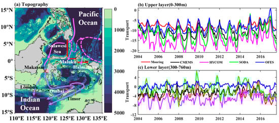
Figure 1.
(a) The topography of the Indonesian sea and the main flow system of the ITF. The pathways of the ITF are shown by magenta solid lines with arrows. The red cross indicates the mooring station in the Makassar Strait. The red and brown solid lines indicate the inflow and outflow channels, respectively. Comparisons of the monthly ITF volume transport in the Makassar strait between the mooring and independent reanalysis datasets in the (b) upper (0–300 m) and (c) lower layers (300–760 m). The black, magenta, green, blue, and red lines indicate the ITF volume transport calculated from CMEMS, HYCOM, SODA, OFES, and mooring in the Labani channel of the Makassar strait [21]. The unit of volume transport is Sv (1 Sv = 106 m3 s−1). Negative values in the ITF inflow and outflow mean southward or westward volume transport (enhanced ITF). The reanalysis datasets were calculated from the section 117°E–119°E, 2.5°S, which is an approximate position at the same latitude as the Makassar Strait mooring position.
The quantitative comparative results are shown in Table 1. It can be found that the correlation coefficients and root mean square error (RMSE) of the four independent reanalysis datasets with the Makassar strait mooring are all larger than 0.75 in the upper layer. Among them, CMEMS and OFES have the largest correlation and the smallest RMSE, which are 0.87 and 1.79 Sv, respectively. The smaller RMSE between OFES and mooring may be caused by the smaller ITF velocity simulated by OFES than other reanalysis datasets and the single or two mooring data points which cannot reflect the overall ITF volume transport. In the lower layer, the HYCOM and SODA show weaker correlations of 0.39 and 0.55. However, the correlation coefficient of the ensemble mean is 0.72. Thus, the simulation biases of the four independent reanalysis datasets can be greatly offset by the ensemble means [30], which are further utilized in decoupling the relative contributions of ENSO and IOD to the ITF volume transport. In addition, the use of the ensemble mean helps to make the results more reliable and does not rely on one type of reanalysis dataset [12,26,27].

Table 1.
The correlation coefficients (R) and root mean square error (RMSE) of the four independent reanalysis datasets with the Makassar strait mooring.
3.2. Definition Sub-Modes of Climate Events
To reveal the different impacts of climate drivers on the entrances and exits, the ITF is divided into two parts: the inflow channels are defined as the Sulawesi Sea (125°E, 1°N–6°N), Maluku Sea (125°E–127.5°E, 0.5°N), and Halmahera Sea (128°E–131°E, 0.5°S) [12]; the outflow channels are defined as the Timor Strait (127.35°E, 8.71°S–10.02°S), the Ombai Strait (125.08°E, 8.33°S–8.83°S), and the Lombok Strait (115.5–116°E, 8.65°S) [27] (Figure 1a).
The complex structures of the flow field in the Sulawesi, Maluku, and Halmahera Seas bring uncertainty to the inflow [2,14,27], which shows a larger variability than the outflow in the upper layer (Figure 2a). The standard deviations are 5.55 Sv and 3.13 Sv in the inflow and outflow channels, respectively. In the lower layer, the ITF inflow and outflow have comparable ranges (Figure 2b), and their standard deviations are 1.50 Sv and 1.12 Sv, respectively.
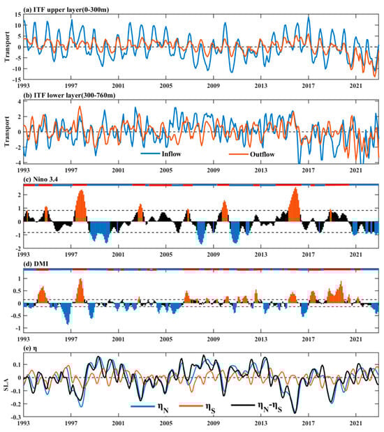
Figure 2.
Monthly time series of average ITF volume transport anomaly in the (a) upper layer (0–300 m) and (b) lower layer (300–760 m) of the four independent reanalysis datasets, (c) Niño 3.4 and (d) DMI indices, and (e) average SLA in the northwest tropical Pacific (NWP, 6°N–16°N, 125°E–155°E), the southeast Indian Ocean (SEI, 6°S–16°S, 85°E–115°E), and the difference between NWP and SEI. The blue and orange solid lines in (a,b) are inflow and outflow, respectively. The unit of volume transport is Sv (1 Sv = 106 m3 s−1). Negative values in the ITF inflow and outflow mean southward or westward volume transport (enhanced ITF). The orange and blue bars in (c,d) indicate absolute values greater than one standard deviation (STD) of the Niño 3.4 index and half of the STD of the DMI index, respectively. The blue, orange, and black solid lines in (e) represent the average SLA for NWP, the average SLA for SEI, and the difference in the average SLA between NWP and SEI, respectively. All the data are smoothed with a 3-month running mean.
Table 2 presents the different types of ENSO and IOD events from Figure 2c,d. In some years, such as 2002–2003, 2004–2005, and 2009–2010, ENSO events occurred with no significant IOD events. IOD events can also occur independently of ENSO events, as they did in 1996–1997, 2005–2006, 2012–2013, and 2017–2018, which are related to the internal dynamics in the Indian Ocean [31,32]. The average ITF volume transport during independent ENSO and IOD events are regarded as the corresponding sub-modes, which are utilized to decouple the relative contributions of concurrent ENSO and IOD events. There are two types of concurrent climate events: El Niño co-occurring with positive IOD, and La Niña co-occurring with negative IOD. The concurrent ENSO and IOD events from 1993 to 2022 are selected according to whether the ENSO (Niño 3.4 > 0.75 STD and lasting more than 6 months) and IOD (DMI > 0.5 STD and lasting more than 5 months) events occurred together. Note that the La Niña co-occurring with negative IOD event in 2016–2017 is also selected [25].
Table 2.
Sub-modes and targets of ENSO and IOD events during the period 1993–2022.
3.3. Contributions of Independent Climate Events to the ITF Transport
After identifying the sub-modes of the ENSO and IOD events, the related ITF volume transport was further clarified.
3.3.1. Independent ENSO Events
In cases of the IOD-independent ENSO events (Figure 3a), the SLAs on the Pacific Ocean side are lower than in an average year (Figure 2e), weakening the ITF transport in the upper layer [2]. The change—a significant decrease—in ITF can be found from September to January in the following year (Figure 3c). Additionally, El Niño reflects a 0–2-month lag in the ITF upper layer transport, with correlation coefficients of 0.82 and 0.66 in the inflow and outflow, respectively (Figure S1 in the Supplementary Materials). The results indicate that the ITF inflow tends to be more affected by ENSO than the ITF outflow. When IOD-independent La Niña events happen (Figure 3b), the changes in ITF in the upper layer are reversed. Influenced by the positive SLA in the Pacific Ocean, the upper layer of the ITF increased significantly from January to September of the following year. It can also be seen that the ITF inflow has a larger increasing amplitude than the ITF outflow (Figure 3d,f). Meanwhile, La Niña has a lag of 6–7 months, with correlation coefficients of 0.77 and 0.68 in the inflow and outflow, respectively (Figure S2 in the Supplementary Materials).
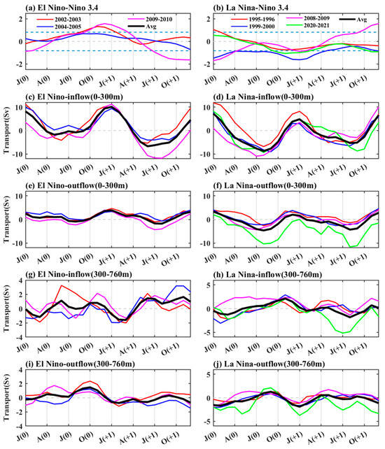
Figure 3.
Changes in (a,b) Niño 3.4 index and ITF volume transport anomaly in the (c,d) inflow (0–300 m), (e,f) outflow (0–300 m), (g,h) inflow (300–760 m), and (i,j) outflow (300–760 m) during IOD-independent El Niño and La Niña events. The red, blue, and magenta solid lines in (a,c,e,g,i) indicate the changes during 2002–2003, 2004–2005, and 2009–2010, respectively. The red, blue, magenta, and green solid lines in (b,d,f,h,j) indicate the changes during 1995–1996, 1999–2000, 2008–2009, and 2020–2021, respectively. The blue dotted lines in (a,b) indicate absolute values greater than one STD of the Niño 3.4 index. The black solid lines in (c–j) indicate the average of ITF volume transport during the IOD-independent El Niño and La Niña events. The horizontal coordinate represents two consecutive months, where (0) represents the first year and (+1) represents the second year. J, A, J, and O indicate January, April, July, and October, respectively.
The opposite performances of the lower and upper layers are suggested to be modulated by Rossby wave propagation [13]. For El Niño, the westward-propagating wave leads to a rise in the depth of the thermocline, thereby increasing the potential height on the inflow side and facilitating a decrease in the ITF volume transport. In this way, the ITF shows an increasing trend from October to February in the following year in the inflow and outflow (Figure 3g,i). The opposite is true for La Niña. During these periods, the ITF shows a decreasing trend in the lower layer (Figure 3h,j). Note that La Niña has a lag of 6 months with the ITF outflow; the correlation coefficient is −0.67.
3.3.2. Independent IOD Events
In cases of ENSO-independent IOD events, in the upper layer, the ITF volume transport is controlled by the interoceanic pressure gradient; meanwhile, in the lower layer, the ITF volume transport is dominated by eastward Kelvin wave propagation. During ENSO-independent positive IOD events (Figure 4a), the equatorial eastward anomaly drives the propagation of the upwelling Kelvin wave in an eastward direction, causing the descent of the upper SLAs and the uplift of the thermocline on the Indian Ocean side [20,26]. This results in a further increase and decrease in the ITF upper (Figure 4c,e) and lower (Figure 4g,i) volume transport. In the upper layer, the ITF’s responses to positive IOD events tend to occur in a timely manner. There are no lags between positive IOD events and the ITF (Figure S3 in the Supplementary Materials). In the lower layer, the ITF volume transport has a lead time of 0–1 and 3–4 months with positive IOD events in the outflow and inflow, respectively.
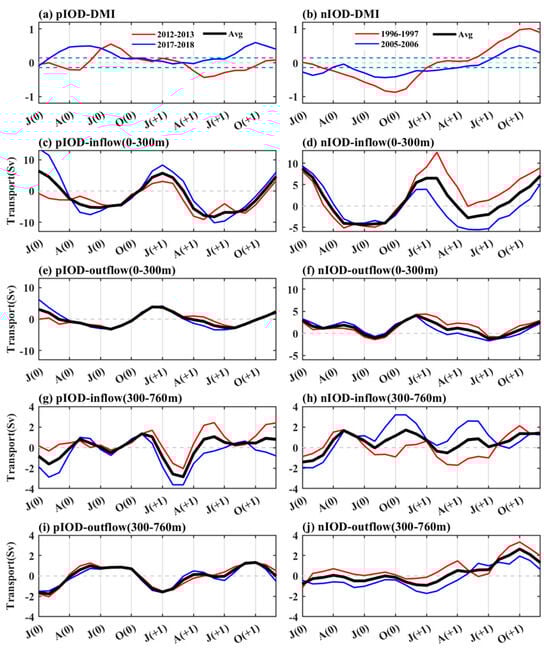
Figure 4.
This figure represents the same principles as Figure 3, except that the changes represented are those occurring during ENSO-independent IOD events. The blue dotted lines in (a,b) represent absolute values greater than half of the STD of the DMI index. The red and blue solid lines in (a,c,e,g,i) represent the changes that occurred during positive IOD (pIOD) events in 2012–2013 and 2017–2018, respectively. The red and blue solid lines in (b,d,f,h,j) represent the changes that occurred during negative IOD (nIOD) events in 1996–1997 and 2005–2006, respectively.
The opposite is true for negative IOD events [25]. Regarding these events (Figure 4b), the event in 1996 was stronger than that in 2005. The ITF upper (Figure 4d,f) and lower layers (Figure 4h,j) have opposite changes from September to April in the following year, which decreased and increased, respectively. The ITF’s outflow showed an earlier response than the inflow. In the upper (lower) layer, the negative IOD has lags of 4 (5) and 3 (3) months with the ITF’s inflow and outflow, respectively (Figure S4 in the Supplementary Materials).
3.4. Decoupling the Relative Contributions during Concurrent ENSO and IOD Events
After separating the respective roles of the ENSO and IOD events on the ITF volume transport, the relative contributions are explored in this section for occasions when they happen concurrently.
3.4.1. Co-Occurring El Niño and Positive IOD Events
First, the contribution of El Niño and positive IOD coupling to ITF volume transport was decoupled and quantified using the CCA analysis method (Table 3).
Table 3.
Relative contributions of ENSO and IOD and the rate between them when El Niño and positive IOD events co-occurred in different years, assessed using CCA analysis.
Compared to IOD, the influence of ENSO on the changes in ITF volume transport was strongest during 1997–1998. The contribution ratio of ENSO and IOD to the upper layer of the ITF inflow reaches 12:1 (Table 3), which indicates that strong El Niño events dominated the changes in the ITF during this period (Figure 5c,d). Similarly, ENSO also made greater contributions to ITF volume transport in 1994–1995 (Figure 5a,b), 2006–2007 (Figure 5e,f), 2015–2016 (Figure 5g,h), and 2018–2019 (Figure 5i,j).
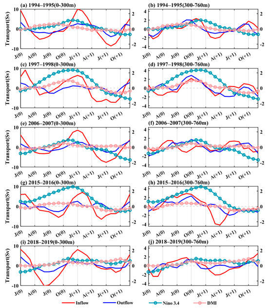
Figure 5.
Changes in the ITF upper layer (0–300 m) volume transport anomaly, Niño 3.4 and DMI indices during (a) 1994–1995 El Niño and positive IOD events co-occurring event. (c,e,g,i) Same as (a) but during 1997–1998, 2006–2007, 2015–2016, and 2018–2019, respectively. (b,d,f,h,j) Same as (a,c,e,g,i) but for the ITF lower layer (300–760 m).
Generally, the contribution ratios of ENSO and IOD to the upper layer of the ITF inflow and outflow volume transport are 5.5:1 and 3.5:1, respectively. The ratios of the contributions of ENSO and IOD to the lower layer of the ITF inflow and outflow volume transport change to 1.7:1 and 1.6:1, respectively. In these years, ENSO plays a dominant role. Compared with the outflow, ENSO makes greater contributions to the upper layer of the ITF volume transport in the inflow side, this is also evidenced in the research of Zhu and Wang [26]. When El Niño and positive IOD events co-occur, positive IOD events usually peak in boreal autumn, while the corresponding El Niño events undergo a strong development period, peaking in boreal winter (Figure 5). At the same time, the ITF volume transport often shows the weakening and strengthening change in the upper and lower layers, respectively.
3.4.2. Co-Occurring La Niña and Negative IOD Events
Compared with the co-occurring positive anomalies of the ENSO and IOD events, an opposite outcome is found during the co-occurrence of La Niña and negative IOD events (Table 4). When La Niña and negative IOD events co-occur, all the climate events develop in the boreal summer; meanwhile, La Niña events peak in boreal autumn (2010–2011 and 2016–2017) and boreal winter (1998–1999 and 2021–2022), and negative IOD events usually peak in boreal autumn (Figure 6). Consequently, the ITF volume transport decreases and increases in the upper and lower layers, respectively.
Table 4.
Relative contributions of ENSO and IOD and the rate between them when La Niña and negative IOD events co-occurred in different years, assessed using CCA analysis.
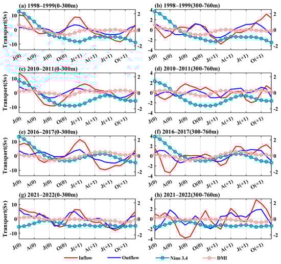
Figure 6.
Changes in ITF upper layer (0–300 m) volume transport anomaly, Niño 3.4 and DMI indices during (a) 1998–1999 La Niña and Negative IOD co-occurring event. (c,e,g) Same as (a) but during 2010–2011, 2016–2017, and 2021–2022, respectively. (b,d,f,h) Same as (a,c,e,g) but for the ITF lower layer (300–760 m).
All four of the independent co-occurring La Niña and negative IOD events show that the negative IOD plays a greater role in the change in ITF volume transport. The ratios of the contributions of ENSO and IOD to the ITF inflow and outflow upper layer transport are 1:6 and 1:6.5, respectively. In the lower layer, the ITF inflow and outflow show that the ratios of the contributions of ENSO and IOD change to 1:4 and 1:3, respectively. It can be found that the IOD has a greater influence on the ITF outflow than it has on the ITF inflow.
Among these influences, a strong negative IOD event coincided with a weaker La Niña event in 2016–2017. Pujiana et al. [25] suggested that the sharp decrease in the ITF upper layer of the Makassar Strait is mostly influenced by the negative IOD event in 2016. In the upper layer, the ratio of the contributions of ENSO and IOD to the ITF inflow and outflow are 1:8.8 and 1:8.3 (Table 4), respectively.
4. Discussion
The CCA results show that in all the years of El Niño and positive IOD co-occurring events, ENSO dominates. In the upper layer, this can be explained by the pressure gradient between the Pacific and Indian Oceans. During the IOD-independent El Niño events (Figure 7a), the difference in the SLA between the NWP and SEI is −0.11 m, indicating a decrease in ITF transport in the upper layer. Meanwhile, the westward propagating Rossby wave increases the ITF lower layer transport by lifting the depth of the thermocline [13], which further enhances the lower pressure gradient between the Pacific and Indian Oceans. For the ENSO-independent positive IOD event shown in Figure 7b, both the NWP and SEI show a positive SLA, and the difference in the SLA is 0.08 m; this is conducive to the formation of an enhanced trend in the upper layer. In the lower layer, the weakening of the ITF transport is closely related to the eastward propagation of the upwelling Kelvin wave [20], which decreases the lower pressure gradients between the Pacific and Indian Oceans by inducing a lift in the depth of the thermocline on the Indian Ocean side.
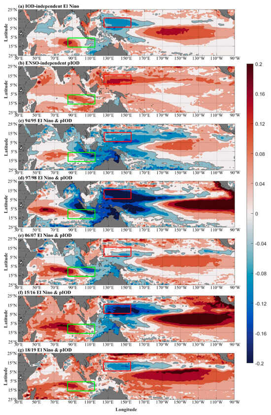
Figure 7.
The distribution of the SLA spatial field during ENSO and IOD positive anomaly events. Sub-modes of (a) IOD-independent El Niño and (b) ENSO-independent positive IOD events. The co-occurrences of El Niño and positive IOD events during (c) 1994–1995, (d) 1997–1998, (e) 2006–2007, (f) 2015–2016, and (g) 2018–2019. The unit of SLA is m. The solid gray lines indicate the contour line with an SLA value of 0. The red and green box areas represent the NWP and SEI regions, respectively.
Specifically, the similar differences in the SLA between the Pacific Ocean and the Indian Ocean during the IOD-independent ENSO events can be found in 1994–1995 (Figure 7c), 1997–1998 (Figure 7d), 2015–2016 (Figure 7f), and 2018–2019 (Figure 7g). The corresponding differences in the SLA between the NWP and SEI are −0.04 m, −0.16 m, −0.23 m, and −0.14 m, respectively. Note that the SLA of NWP reached a minimum (−0.20 m) in 1997–1998, and this may be the main reason that explains why it has a maximum ratio of contributions of ENSO and IOD (12:1) in the upper layer of the ITF inflow. Note that the calculated ratio values might considerably be affected by estimation errors. When one of two compared values is close to zero, the ratio might give misleading characterization much more easily than in other cases. Compared to IOD, the strong dominant role of ENSO in 1997–1998 corresponds to that during 1993–2000 in the study of Li et al. (2023) [27]. Note that in 2006–2007, the difference in SLA between the NWP and SEI is −0.01 m, which is relatively lower than in the other events (2.4:1). The difference between this part and Li et al. (2023) [27] mainly comes from the fact that the method used in this study targets a certain period rather than the whole period.
During La Niña and negative IOD coupling events, IOD shows a greater influence on the outflow. This mechanism can also be explained by the SLA differences between NWP and SEI. For the independent ENSO and IOD negative anomaly events, the SLA differences between the NWP and SEI are 0.04 and −0.02, respectively (Figure 8a,b). When La Niña and negative IOD events occur concurrently, the differences in SLA between the NWP and SEI are 0.07 m, 0.05 m, −0.03 m, and −0.02 m in 1998–1999 (Figure 8c), 2010–2011 (Figure 8d), 2016–2017 (Figure 8e), and 2021–2022 (Figure 8f), respectively. This difference is reflected in the changes in the strength of La Niña and negative IOD events. Even though the two typical SLAs representing the Pacific and Indian Ocean regions differ, the changes in ITF volume transport over the corresponding periods reflect a closer alignment with the ENSO-independent negative IOD events. The decreasing and increasing trends are obvious in the upper and lower layers, respectively. In 2016–2017, the ratio of the contributions of IOD and ENSO events reached above 8:1, which further confirms that negative IOD events have a larger contribution than La Niña events [25,27].
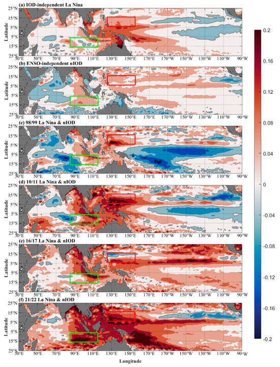
Figure 8.
Same as Figure 7 but for ENSO and IOD negative anomaly events. Sub-modes of (a) IOD-independent La Niña and (b) ENSO-independent negative IOD events. The co-occurrences of La Niña and negative IOD events during (c) 1998–1999, (d) 2010–2011, (e) 2016–2017, and (f) 2021–2022.
5. Conclusions
In this study, the improved CCA analysis method and four independent reanalysis datasets were employed to reveal the roles of climate drivers in modulating the ITF volume transport when two climate events co-occurred. Validation results of the reanalysis datasets show that OFES, CMEMS, and SODA have a greater performance in the upper, lower, and lower layers, respectively. HYCOM overestimates the ITF volume transport, and its simulation is weak in the lower layer. However, by synthesizing the four independent reanalysis datasets, the ensemble meaning results show a good correspondence with the mooring data.
By using the CCA analysis method, the sub-modes of the ENSO and IOD events were identified. When an ENSO sub-mode occurs, it has a greater influence on the ITF inflow than it does on the ITF outflow. When an IOD sub-mode occurs, the ITF upper layer has no lag with positive IOD events. The ITF outflow has an earlier and stronger response than that in the ITF inflow during the negative IOD events.
The CCA results show that ITF volume transport has an asymmetric response to co-occurring ENSO-IOD events. In cases of the co-occurrence of El Niño and positive IOD events, ENSO dominates the changes in the ITF volume transport, and it plays a greater role in the inflow than in the outflow. The large differences in SLA between the NWP and SEI dominate the changes in the ITF volume transport in the upper layer, which is caused by the El Niño events. In the lower layer, the westward propagating Rossby wave plays a role in lifting the depth of the thermocline, increasing further the ITF volume transport. In the typical 1997–1998 event, the ratio of contributions of ENSO and IOD reaches 12:1 in the upper layer of the ITF inflow. In cases of the co-occurrence of La Niña and negative IOD events, IOD dominates the changes in the ITF volume transport, which shows greater influence on the outflow. In the typical 2016–2017 event [25], the ratio of the contributions of IOD and ENSO reaches more than 8:1 in the upper layer.
The effects of the ENSO and IOD climate forcing on the ITF volume transport are often nonlinear and complex [27,33], making their contributions difficult to quantify. However, this problem can be addressed by utilizing the CCA analysis method proposed in this study. The idea of using the sub-modes of historical events to decouple and quantify the nonlinear processes, acknowledging the roles of individual influencing factors, provides promising new access to perform attribution studies in this research field.
Supplementary Materials
The following supporting information can be downloaded at https://www.mdpi.com/article/10.3390/rs16183395/s1. Figure S1. Lead-lag correlations between ITF volume transport and Niño 3.4 index during IOD-independent El Niño events. Figure S2. Lead-lag correlations between ITF volume transport and Niño 3.4 index during IOD-independent La Niña events. Figure S3. Lead-lag correlations between ITF volume transport and DMI index during ENSO-independent Positive IOD events. Figure S4. Lead-lag correlations between ITF volume transport and DMI index during ENSO-independent Negative IOD events.
Author Contributions
Methodology, A.L. and Y.Z.; software, A.L.; validation, A.L. and Y.Z.; data curation, A.L.; writing—original draft, A.L.; writing—review & editing, Y.Z. and T.X.; supervision, Y.Z., M.H. and T.X.; funding acquisition, T.X. and J.W. All authors have read and agreed to the published version of the manuscript.
Funding
This work was financially supported by the National Key R&D Program of China (2019YFA0606702), Laoshan Laboratory (No. LSKJ202202704), and the Strategic Priority Research Program of the Chinese Academy of Sciences (Grant XDB42000000).
Data Availability Statement
The Makassar Mooring data are available at https://academiccommons.columbia.edu/doi/10.7916/d8-p78a-zm51 (accessed on 13 November 2022). The CMEMS and the SLA data used in this study are available at https://resources.marine.copernicus.eu (accessed on 10 August 2022). The HYCOM, SODA 3.4.2, and OFES data are available at https://apdrc.soest.hawaii.edu/data/data.php (accessed on 1 October 2022). The Niño 3.4 El Niño and DMI climate indices are available at https://psl.noaa.gov/data/climateindices/list/ (accessed on 12 October 2022). The bathymetry ETOPO1 data are available at https://www.opentopodata.org/datasets/etopo1/ (accessed on 10 August 2022).
Acknowledgments
We would like to thank the editor for editing and the three anonymous reviewers for reviewing.
Conflicts of Interest
The authors declare no conflict of interest.
References
- Gordon, A.L.; Sprintall, J.; Van Aken, H.M.; Susanto, D.; Wijffels, S.; Molcard, R.; Ffield, A.; Pranowo, W.; Wirasantosa, S. The Indonesian throughflow during 2004–2006 as observed by the INSTANT program. Dyn. Atmos. Oceans 2010, 50, 115–128. [Google Scholar] [CrossRef]
- Liu, Q.Y.; Feng, M.; Wang, D.; Wijffels, S. Interannual variability of the Indonesian Throughflow transport: A revisit based on 30 year expendable bathythermograph data. J. Geophys. Res. Oceans 2015, 120, 8270–8282. [Google Scholar] [CrossRef]
- Sprintall, J.; Gordon, A.L.; Wijffels, S.E.; Feng, M.; Hu, S.; Koch-Larrouy, A.; Phillips, H.; Nugroho, D.; Napitu, A.; Pujiana, K. Detecting change in the Indonesian seas. Front. Mar. Sci. 2019, 6, 257. [Google Scholar] [CrossRef]
- Sprintall, J.; Wijffels, S.E.; Molcard, R.; Jaya, I. Direct estimates of the Indonesian Throughflow entering the Indian Ocean: 2004–2006. J. Geophys. Res. Oceans 2009, 114, C7. [Google Scholar] [CrossRef]
- Susanto, R.D.; Ffield, A.; Gordon, A.L.; Adi, T.R. Variability of Indonesian throughflow within Makassar strait, 2004–2009. J. Geophys. Res. Oceans 2012, 117, C9. [Google Scholar] [CrossRef]
- Wijffels, S.E.; Meyers, G.; Godfrey, J.S. A 20-yr average of the Indonesian Throughflow: Regional currents and the interbasin exchange. J. Phys. Oceanogr. 2008, 38, 1965–1978. [Google Scholar] [CrossRef]
- Du, Y.; Qu, T. Three inflow pathways of the Indonesian throughflow as seen from the simple ocean data assimilation. Dyn. Atmos. Oceans 2010, 50, 233–256. [Google Scholar] [CrossRef]
- Godfrey, J. The effect of the Indonesian throughflow on ocean circulation and heat exchange with the atmosphere: A review. J. Geophys. Res. Oceans 1996, 101, 12217–12237. [Google Scholar] [CrossRef]
- Gordon, A.L. Interocean exchange of thermocline water. J. Geophys. Res. Oceans 1986, 91, 5037–5046. [Google Scholar] [CrossRef]
- Gordon, A.L. Oceanography of the Indonesian seas and their throughflow. Oceanography 2005, 18, 14–27. [Google Scholar] [CrossRef]
- Hu, S.; Zhang, Y.; Feng, M.; Du, Y.; Sprintall, J.; Wang, F.; Hu, D.; Xie, Q.; Chai, F. Interannual to decadal variability of upper-ocean salinity in the southern Indian Ocean and the role of the Indonesian Throughflow. J. Clim. 2019, 32, 6403–6421. [Google Scholar] [CrossRef]
- Li, M.; Gordon, A.L.; Gruenburg, L.K.; Wei, J.; Yang, S. Interannual to decadal response of the Indonesian throughflow vertical profile to Indo-Pacific forcing. Geophys. Res. Lett. 2020, 47, e2020GL087679. [Google Scholar] [CrossRef]
- Sprintall, J.; Gordon, A.L.; Koch-Larrouy, A.; Lee, T.; Potemra, J.T.; Pujiana, K.; Wijffels, S.E. The Indonesian seas and their role in the coupled ocean–climate system. Nat. Geosci. 2014, 7, 487–492. [Google Scholar] [CrossRef]
- Yuan, D.; Yin, X.; Li, X.; Corvianawatie, C.; Wang, Z.; Li, Y.; Yang, Y.; Hu, X.; Wang, J.; Tan, S. A Maluku Sea intermediate western boundary current connecting Pacific Ocean circulation to the Indonesian Throughflow. Nat. Commun. 2022, 13, 2093. [Google Scholar] [CrossRef]
- Cai, W.; Sullivan, A.; Cowan, T. Interactions of ENSO, the IOD, and the SAM in CMIP3 models. J. Clim. 2011, 24, 1688–1704. [Google Scholar] [CrossRef]
- Gordon, A.L.; Susanto, R.D.; Ffield, A. Throughflow within makassar strait. Geophys. Res. Lett. 1999, 26, 3325–3328. [Google Scholar] [CrossRef]
- Hu, S.; Sprintall, J. Interannual variability of the Indonesian Throughflow: The salinity effect. J. Geophys. Res. Oceans 2016, 121, 2596–2615. [Google Scholar] [CrossRef]
- Meyers, G. Variation of Indonesian throughflow and the El Niño-southern oscillation. J. Geophys. Res. Oceans 1996, 101, 12255–12263. [Google Scholar] [CrossRef]
- Sprintall, J.; Révelard, A. The Indonesian throughflow response to Indo-Pacific climate variability. J. Geophys. Res. Oceans 2014, 119, 1161–1175. [Google Scholar] [CrossRef]
- Yuan, D.; Wang, J.; Xu, T.; Xu, P.; Hui, Z.; Zhao, X.; Luan, Y.; Zheng, W.; Yu, Y. Forcing of the Indian Ocean dipole on the interannual variations of the tropical Pacific Ocean: Roles of the Indonesian throughflow. J. Clim. 2011, 24, 3593–3608. [Google Scholar] [CrossRef]
- Gordon, A.L.; Napitu, A.; Huber, B.A.; Gruenburg, L.K.; Pujiana, K.; Agustiadi, T.; Kuswardani, A.; Mbay, N.; Setiawan, A. Makassar Strait throughflow seasonal and interannual variability: An overview. J. Geophys. Res. Oceans 2019, 124, 3724–3736. [Google Scholar] [CrossRef]
- Feng, M.; Meyers, G.; Wijffels, S. Interannual upper ocean variability in the tropical Indian Ocean. Geophys. Res. Lett. 2001, 28, 4151–4154. [Google Scholar] [CrossRef]
- Murtugudde, R.; Busalacchi, A.J.; Beauchamp, J. Seasonal-to-interannual effects of the Indonesian throughflow on the tropical Indo-Pacific Basin. J. Geophys. Res. Oceans 1998, 103, 21425–21441. [Google Scholar] [CrossRef]
- Saji, N.; Goswami, B.N.; Vinayachandran, P.; Yamagata, T. A dipole mode in the tropical Indian Ocean. Nature 1999, 401, 360–363. [Google Scholar] [CrossRef]
- Pujiana, K.; McPhaden, M.J.; Gordon, A.L.; Napitu, A.M. Unprecedented response of Indonesian throughflow to anomalous Indo-Pacific climatic forcing in 2016. J. Geophys. Res. Oceans 2019, 124, 3737–3754. [Google Scholar] [CrossRef]
- Zhu, Q.; Wang, C. Contributions of Indo-Pacific Forcings to Interannual Variability of the Indonesian Throughflow in the Upper and Lower Layers. J. Geophys. Res. Oceans 2024, 129, e2023JC020306. [Google Scholar] [CrossRef]
- Li, A.; Zhang, Y.; Hong, M.; Shi, J.; Wang, J. Relative importance of ENSO and IOD on interannual variability of Indonesian Throughflow transport. Front. Mar. Sci. 2023, 10, 1182255. [Google Scholar] [CrossRef]
- Zhuang, Y.; Fu, R.; Santer, B.D.; Dickinson, R.E.; Hall, A. Quantifying contributions of natural variability and anthropogenic forcings on increased fire weather risk over the western United States. Proc. Natl. Acad. Sci. USA 2021, 118, e2111875118. [Google Scholar] [CrossRef]
- Gordon, A.; Susanto, R.; Ffield, A.; Huber, B.; Pranowo, W.; Wirasantosa, S. Makassar Strait throughflow, 2004 to 2006. Geophys. Res. Lett. 2008, 35, 24. [Google Scholar] [CrossRef]
- Balmaseda, M.A.; Hernandez, F.; Storto, A.; Palmer, M.; Alves, O.; Shi, L.; Smith, G.C.; Toyoda, T.; Valdivieso, M.; Barnier, B. The ocean reanalyses intercomparison project (ORA-IP). J. Oper. Oceanogr. 2015, 8 (Supp. S1), s80–s97. [Google Scholar] [CrossRef]
- Du, Y.; Cai, W.; Wu, Y. A new type of the Indian Ocean Dipole since the mid-1970s. J. Clim. 2013, 26, 959–972. [Google Scholar] [CrossRef]
- Polonsky, A.; Torbinsky, A. The IOD–ENSO interaction: The role of the Indian Ocean current’s system. Atmosphere 2021, 12, 1662. [Google Scholar] [CrossRef]
- Wang, J.; Zhang, Z.; Li, X.; Wang, Z.; Li, Y.; Hao, J.; Zhao, X.; Corvianawatie, C.; Surinati, D.; Yuan, D. Moored observations of the timor passage currents in the Indonesian seas. J. Geophys. Res. Oceans 2022, 127, e2022JC018694. [Google Scholar] [CrossRef]
Disclaimer/Publisher’s Note: The statements, opinions and data contained in all publications are solely those of the individual author(s) and contributor(s) and not of MDPI and/or the editor(s). MDPI and/or the editor(s) disclaim responsibility for any injury to people or property resulting from any ideas, methods, instructions or products referred to in the content. |
© 2024 by the authors. Licensee MDPI, Basel, Switzerland. This article is an open access article distributed under the terms and conditions of the Creative Commons Attribution (CC BY) license (https://creativecommons.org/licenses/by/4.0/).