The Operational and Climate Land Surface Temperature Products from the Sea and Land Surface Temperature Radiometers on Sentinel-3A and 3B

Abstract

Land Surface Temperature (LST) is integral to our understanding of the radiative energy budget of the Earth’s surface since it provides the best approximation to the thermodynamic temperature that drives the outgoing longwave flux from surface to atmosphere. Since 5 July 2017, an operational LST product has been available from the Sentinel-3A mission, with the corresponding product being available from Sentinel-3B since 17 November 2018. Here, we present the first paper describing formal products, including algorithms, for the Sea and Land Surface Temperature Radiometer (SLSTR) instruments onboard Sentinel-3A and 3B (SLSTR-A and SLSTR-B, respectively). We evaluate the quality of both the Land Surface Temperature Climate Change Initiative (LST_cci) product and the Copernicus operational LST product (SL_2_LST) for the years 2018 to 2021. The evaluation takes the form of a validation against ground-based observations of LST across eleven well-established in situ stations. For the validation, the mean absolute daytime and night-time difference against the in situ measurements for the LST_cci product is 0.77 K and 0.50 K, respectively, for SLSTR-A, and 0.91 K and 0.54 K, respectively, for SLSTR-B. These are an improvement on the corresponding statistics for the SL_2_LST product, which are 1.45 K (daytime) and 0.76 (night-time) for SLSTR-A, and 1.29 K (daytime) and 0.77 (night-time) for SLSTR-B. The key influencing factors in this improvement include an upgraded database of reference states for the generation of retrieval coefficients, higher stratification of the auxiliary data for the biome and fractional vegetation, and enhanced cloud masking.

1. Introduction

Land surface temperature (LST) is the radiative skin temperature of the land. It is derived from solar radiation and influences the partitioning of energy into sensible heat flux, latent heat flux, and the heat flux into the ground [1,2]. It can be measured from satellites, aircraft, the ground, in thermal infrared (TIR), or microwave, and is the best approximation to the thermodynamic temperature based on a measure of radiance [3].

Earth Observation (EO) satellite instruments operate in the infrared measure top-of-atmosphere (TOA) radiances, which are a combination of the upwelling radiance emitted by the ground, the upwelling radiance emitted by the atmosphere, and the downwelling radiance emitted by the atmosphere and reflected by the ground. Accuracy of LST retrievals is, however, difficult to achieve due to emissivity variability and atmospheric effects. Land surface emissivities are more variable than those over the sea due to surface heterogeneity. Such variability also increases for larger viewing angles and in regions of high topographic variance. If emissivity corrections are not accurately dealt with, then biases of several degrees can result [4]. Atmospheric effects on the derivation of LST include the presence of clouds or aerosols, which can give a negative bias to the underlying LST if not corrected for. Most LST algorithms usually operate in the 8–13 μm TIR range where atmospheric transmission is high to minimise the effects of the atmosphere [5]. Further justification for the retrieval of LST in this TIR range is that according to Wien’s Displacement Law, the peak of the Earth’s spectral radiance at an ambient temperature of 300 K occurs at approximately 9.6 µm [6]. Even so, attenuation at these wavelengths can still be significant.

The most commonly applied operational approach to resolve this is the split-window technique [7,8,9,10,11,12,13], which solves two simultaneous equations for TOA brightness temperatures—at approximately 11 µm and 12 µm wavelengths—based on a priori knowledge of the surface emissivity from land cover classification. The rationale here is that atmospheric attenuation is a function of the differential absorption at each channel wavelength [13]. If neither emissivity variability nor atmospheric effects are accounted for, then retrieval errors up to 12 K may result [14,15]. Other methods for LST retrieval include the single channel approach [16,17], the Temperature Emissivity Separation (TES) method [18,19], and the physics-based day/night (D/N) approach [20]. A recent review of the different approaches is presented in [21]. For instruments with two thermal channels when operating with comprehensive coefficients, it has been shown [22] that split window algorithms can be the most effective. These algorithms do not require accurate atmospheric profiles, unlike single-channel algorithms. TES methodology requires at least three thermal channels so is not applicable for instruments with just two thermal channels. The D/N approach requires accurate geometric registration and similar observation angles between day and night, making the approach more challenging to implement in an operational environment [21].

The Sea and Land Surface Temperature Radiometer (SLSTR) on the Copernicus Sentinel-3 mission responds to the requirements for long-term (>20 years) operational and near-real-time monitoring of the Earth’s surface. The instrument measures Sea and Land Surface Temperature with high-end accuracy and reliability [23] in support of environmental and climate monitoring under the remit of the European Union Copernicus Programme. Both Sentinel-3A (launched on 16 February 2016) and 3B (launched on 25 April 2018) will deliver operational LST for the next few years with follow-on units 3C and 3D also approved. SLSTR provides a continuation of the series of Along Track Scanning Radiometers (ATSRs) [24], the last of which, AATSR (Advanced Along Track Scanning Radiometer), stopped delivering data on 8 April 2012 with the failure of the Envisat platform. Both SLSTR and the ATSRs use conical scanning, which facilitates dual view capability, with precise thermal control of the instrument and accurate radiometry through a highly stable in-flight calibration scheme [25]. The near nadir swath is 1420 km, with the backward view being 750 km. There are nine spectral channels for SLSTR in the visible, short-wave infrared, and three co-aligned TIR bands centred at 3.7 µm, 10.8 µm, and 12 µm. Near-complete global coverage each day is delivered with the two satellites (Sentinel-3A and 3B). Together, SLSTR and the ATSRs represent a basis for climate data, building on the quality achieved for sea surface temperature [26].

Ensuring data quality validation is a critical part of developing any satellite product, although surface heterogeneity ensures this is a challenging undertaking for LST. As such, validation sites should encompass areas larger than a satellite pixel size, with a homogeneous land cover [27,28]. This minimizes the spatial variability in temperature and emissivity within the satellite pixel, reducing the uncertainty in upscaling in situ measurements at a single point to area-averaged satellite measurements. Numerous LST validation studies have been carried out over such surfaces [28,29,30,31,32,33,34,35]. Although the ideal is to use homogeneous sites, a wider set of in situ stations has become standard for LST as the overall result can be more meaningful statistically [12,36,37,38,39,40].

For any operational product that is disseminated to the user community with near-real-time (NRT) or non-time critical (NTC) timeliness, the ability to evaluate the quality of the product through routine validation is essential. SLSTR is designed to retrieve global Land Surface Temperature to an accuracy of less than 1 K. Routine validation to assess this accuracy requirement has been carried out within the framework of the Sentinel-3 Mission Performance Centre, which is responsible for the quality of the products generated for the mission. Previous validation of the SL_2_LST product has been limited to just a few sites over limited date ranges [41,42,43,44]. Here, we perform a first systematic multi-year validation over multiple in situ stations for Sentinel-3A and 3B SLSTR products (SLSTR-A and SLSTR-B).

This paper presents for the first time the results of the validation of the operational LST product (SL_2_LST) from SLSTR and compares these with equivalent validation for the SLSTR LST product from the ESA Land Surface Temperature Climate Change Initiative (LST_cci). We describe the essential aspects of the split-window retrieval algorithm implemented in the operational Instrument Processing Facility (IPF) for SLSTR, and the optimized cloud detection scheme also implemented in the IPF. Recognizing the motivation to produce climate-quality long-term global datasets [45], we also consider the equivalent processing undertaken within LST_cci for climate-quality data.

2. Materials and Methods

2.1. SLSTR LST Products Overview

Two separate data records are publicly available for SLSTR: the operational near-real-time/non-time-critical (NRT/NTC) product (SL_2_LST) for SLSTR-A and SLSTR-B; and the climate product (LST_cci), which is available with a latency of several months. These products are freely available from Copernicus, in the case of SL_2_LST, and from ESA, in the case of LST_cci, in easily accessible NetCDF format. They offer near-complete global coverage each day at 1 km spatial resolution. Long-term operational continuity of the Sentinels through the Copernicus Programme is assured with the next generation of missions already in the early development phases. While the SLSTRs have at present a short data history, they are successor missions to the ATSR series enabling long-term multi-mission data records to be created. An advantage of the LST_cci products is that they provide climate quality data, where the whole mission is processed consistently to eliminate non-climatic trends or step changes. One advantage of the SL_2_LST products is that they provide data in near-real time, but they compromise on quality compared to the LST_cci products. Optimal auxiliary datasets are not available within the NRT/NTC timeframe for the SL_2_LST products. Furthermore, there is inertia in the operational system when instituting changes to the algorithm, and, indeed, some operational users may prefer for changes not to be made. This paper presents a comparison of these SLSTR products, which is crucial for users of LST data to understand the advantages and disadvantages of these products. An overview of the methods and processes for generating the SLSTR Level-2 LST products is illustrated in Figure 1, with detailed descriptions of the individual steps presented in the sections below.

The SL_2_LST operational product is derived using an established retrieval algorithm providing continuity from the LST products available from ESA for the ATSR series of instruments. The LST_cci product also uses the same functional form of the retrieval algorithm but with differences in auxiliary data and the generation of the retrieval coefficients. LST from Sentinel-3A became operationally available from 5 July 2017. LST from Sentinel-3B became operationally available from 25 February 2019. Here, we evaluate both products from the start of the respective instrument operations through to end-2021 capturing inter- and intra-annual cycles.

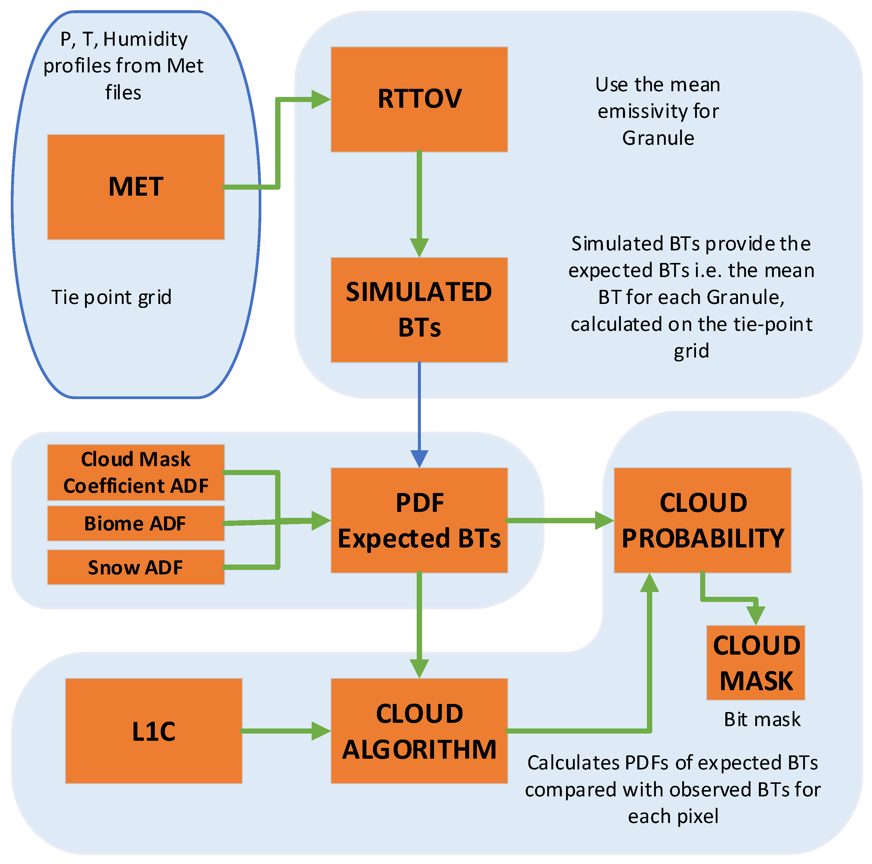
2.1.1. Algorithm Overview

Both the SL_2_LST operational product and the LST_cci product use the same functional form of the retrieval algorithm [11,12,22,46], which maintains the heritage from the ATSRs:

$$\begin{array}{c}LST=d\left(\sec \left(\theta \right)-1\right)pw+{fa}_{v,i}+\left(1-f\right)a_{s,i}\\ +({fb}_{v,i}+\left(1-f\right)b_{s,i}){\left(T_{11}-T_{12}\right)}^{(1/(\mathrm{c}\mathrm{o}\mathrm{s}(\theta /m)\left)\right)}\\ +\left({fb}_{v,i}+\left(1-f\right)b_{s,i}+{fc}_{v,i}+\left(1-f\right)c_{s,i}\right)T_{12}\end{array}$$

(1)

where the retrieval coefficients a_v,i, a_s,i, b_v,i b_s,i, c_v,i, and c_s,i, which are determined for each combination of biome (i), under bare soil (s), fully vegetated conditions (v), and time of day (day or night), act on the brightness temperatures (BTs) for the channels centred around 11 µm (T₁₁) and 12 µm (T₁₂). Surface and atmospheric variability are included through the fractional vegetation cover (f) and precipitable water (pw), respectively. The algorithm formulation means that the emissivity of the Land Surface is implicitly accounted for in the coefficient generation through the radiative transfer simulation process. Parameterization to account for the increase in atmospheric attenuation with respect to satellite zenith angle (θ) is controlled through m and d. Since attenuation due to water vapor is greater at 12 μm than at 11 μm, the parametrization introduces a weak non-linearity as a function of the 11 μm–12 μm BT difference. A full description of the algorithm can be found in [12].

The retrieval coefficients for the algorithm are determined through linear regression between simulated BTs and corresponding skin temperatures for cases of f = 0 and f = 1. A radiative transfer model is used to simulate the BTs. In this case, the fast radiative transfer model RTTOV (Radiative Transfer for TOVS) v12.3 is used [47,48]. It is an efficient forward model for radiative transfer in the visible, TIR, and microwave. A database of reference states from atmospheric profiles and respective surface conditions is used, which provides the inputs to the BT simulations. Requirements for the database include vertical atmospheric profiles of temperature, water vapor, and ozone; surface and near-surface meteorological conditions; surface emissivities; and the instrument spectral response functions [12,22,49].

For the SL_2_LST operational product, a uniform random sampling distribution is used across the land and ice surfaces to select clear-sky profile data for each biome class, with a temporal sampling of the 15th day of every month covering the years 2002–2011. Atmospheric profiles are from the European Centre for Medium-Range Weather Forecasts (ECMWF) ERA-Interim reanalysis [50], with emissivity from the University of Wisconsin (UWIREMIS) dataset, which was known as CIMSS [51]. Full details are presented in [12].

For the LST_cci product, the database of reference states [22] is constructed in a different way with updated input data. For instance, ECMWF ERA5 data are used for the profiles [52] with emissivities coming from the Combined ASTER MODIS Emissivity over Land (CAMEL) V2 dataset, which is available from 2000 to 2016 [53,54]. These input data are first gridded to 5 × 5° cells with the mean total column water vapour (TCWV) calculated. This mean is compared to all TCWV values over the 5 × 5° cell. The profile selected in the spatial sampling is that where the TCWV value most closely matches the mean for the cell. The LST_cci database of reference states covers the years 2001–2016, from which data are selected on the 5th, 15th, and 25th of each month according to this spatial sampling [22].

2.1.2. Auxiliary Data Files (ADFs)

Four different ADFs are input to the processing of the LST for SLSTR [12,22]: (i) biome classification; (ii) fractional vegetation; (iii) precipitable water; and (iv) snow coverage. The SL_2_LST product uses a biome classification, which is a variant of the 2006 Globcover product [55] where the original single bare soil class is subdivided into the most dominant soil types [12]. The resultant classification consists of 27 classes for land and inland/coastal water. For LST_cci, the biome classification is a variant of the Land Cover CCI dataset [56]. The original soil classes have also been subdivided as per [12] to give 42 overall classes. The different biome classifications are presented in Appendix A.

Fractional vegetation cover is derived from the Copernicus Global Land Services (CGLS) FCOVER dataset [57]. For SL_2_LST, a 10-day climatological fractional vegetation cover auxiliary dataset is used. This is derived from the 1 km FCOVER archive dataset. A more dynamic approach is used for LST_cci, which tries to capture the change every 10 days for the current year. Here, the CGLS 300 m FCOVER dataset is used, which is synthesized from data acquired from the Ocean and Land Colour Instrument (OLCI).

Water vapour inputs to the retrieval algorithm are acquired from monthly European Centre for Medium-Range Weather Forecasts (ECMWF) climatology. For SL_2_LST, the source is the ERA-Interim reanalysis [50], with 6-hourly monthly climatology from 2002 to 2011 at 4 synoptic times (00UTC, 06UTC, 12UTC, and 18UTC). For LST_cci, we use ERA5 data [52] coincident in space and time with the corresponding instrument tie-point grid.

Snow coverage is acquired from daily Interactive Multisensor Snow and Ice Mapping System (IMS) maps for the Northern Hemisphere [58]. These are produced by the United States National Snow and Ice Data Center (NSIDC) from satellite and in situ data on an equal area polar stereographic grid. The SLSTR product uses the latest 1 km data, which have been produced since 2014.

2.1.3. Cloud Clearing

A probabilistic approach is used for SLSTR cloud clearing. This is semi-Bayesian and simulates the probability of clear-sky conditions [12,59]. Here, we describe a brief overview. Clear-sky conditions are simulated using radiative transfer modelling from ERA5 atmospheric profiles [52] coincident in space and time with the corresponding instrument tie-point grid. The SLSTR tie-point grid corresponds to 16 pixels across-track and 1 pixel along-track. The mapping of the atmospheric profiles from ECMWF is through bilinear interpolation of profiles and temporal interpolation between 6-hourly fields. A pixel cloud mask is derived using information from probability density functions, whereby a normal distribution is assumed, with the mean being the simulated BT or brightness temperature differences (BTDs) for the tie-point and the standard deviation being the observational climatology for the specific biome, month, and day/night condition. Different tests of BTs or BTDs, for the SLSTR S8 (11 µm) and S9 (12 µm) channels with the use of the S7 (3.7 µm) channel at night, are considered and a pixel is masked as cloudy if the combined probabilities are less than a 95% confidence threshold. The same approach is taken for both the SL_2_LST and LST_cci products. However, for LST_cci, new cloud mask coefficient PDFs, which are shown in Figure 2, have been derived for each biome of the new biome classification scheme. The expectation is that the more detailed stratification of the cloud histograms would increase the distinction between clear and cloudy pixels, thus improving the performance of the cloud detection scheme. Furthermore, the use of improved profile data, as stated in the algorithm overview section, means a better representation of the BTs and BTDs is produced for the decision process.

2.1.4. Uncertainty Model

The state-of-the-art approach for LST uncertainty, introduced in [60] using concepts first presented for Sea Surface Temperature and for building fundamental climate data records [61,62] has been implemented both operationally for the SL_2_LST product and for LST_cci. This takes a measurement equation, in this case, the LST retrieval equation, and assesses all of the uncertainties associated with each component of the equation. Sources of uncertainty are listed in an error effects table, with the correlation length scale of each error effect estimated, and linked to the part of the measurement equation where they are introduced [63]. This approach produces uncertainties for uncorrelated, locally systematic, and large-scale systematic components per pixel.

The details of each uncertainty component are described in [46,60] but are summarised here and illustrated in Figure 3. The random uncertainty per pixel $u_{ran}\left(x\right)$ (Figure 3, top-right) is given by

$$u_{ran,T}\left(x\right)=\sqrt{\sum _{i=1}^n{\left({\displaystyle \frac{\partial R}{{\partial T}_i}}{u}_{ran}(T_i)\right)}^2}$$

(2)

where $u_{ran}\left(T_i\right)$ is the noise equivalent differential temperature (NEDT) for brightness temperature channel i and R represents the LST retrieval algorithm. The estimation of the locally correlated surface uncertainty per pixel $u_{loc,sfc}\left(x\right)$ (Figure 3, bottom-left) is given by

$$u_{loc,sfc}\left(x\right)={\displaystyle \frac{\partial R}{\partial f}}{u}_{loc}(f)$$

(3)

where $u_{loc}\left(f\right)$ is the error in fractional vegetation cover input state per pixel from [57,64].

Two specific evolutions have been made to the initial model of [60] and implemented for both SL_2_LST and LST_cci products. Firstly, an estimation of the uncertainty due to direct TCWV input per pixel ($u_{loc,atm,alg}$). We apply the partial derivative of the LST retrieval algorithm (Equation (1)) with respect to TCWV for each pixel:

$$u_{loc,atm,alg}\left(x\right)={\displaystyle \frac{\partial R}{\partial tcwv}}{u}_{loc}(tcwv)$$

(4)

where $u_{loc}\left(tcwv\right)$ is the instantaneous TCWV distribution to a climatology of this spread that depends on the actual TCWV, latitude, and month. The total locally correlated atmosphere uncertainty $u_{loc,atm}\left(x\right)$ (Figure 3, center-right) then becomes the combination in quadrature of $u_{loc,atm,alg}\left(x\right)$ and $u_{loc,atm,fit}\left(x\right)$. This latter term, which is the estimate of the locally correlated atmosphere “fitting” uncertainty for every pixel, is given by

$$u_{loc,atm,fit}\left(x\right)=\sqrt{Var(\widehat{x}-x_{in})}$$

(5)

Secondly, we also quantify the uncertainty from errors that arise from the pre-launch calibration [25]. This radiometric uncertainty $u_{loc,T}\left(x\right)$ (Figure 3, center-left) is derived as a function of scene brightness temperature using the calibration information in the Level 1 quality annotation files. We apply the partial derivative of the LST retrieval algorithm (Equation (1)) with respect to each SLSTR channel i for each pixel:

$$u_{loc,T}\left(x\right)=\sqrt{\sum _{i=1}^n{\left({\displaystyle \frac{\partial R}{{\partial T}_i}}{u}_{loc}(T_i)\right)}^2+2\sum _{i=1}^{n-1}\sum _{j=i+1}^n{\displaystyle \frac{\partial R}{\partial T_i}}{\displaystyle \frac{\partial R}{\partial T_j}}{u}_{loc}(T_i,T_j)}$$

(6)

where $u_{loc}\left(T_i\right)$ is the radiometric uncertainty for brightness temperature channel i. The covariance term is included due to correlation between channels for the radiometric calibration.

A final source of uncertainty is geolocation (Figure 3, bottom-right). This is due to both (i) a correction of the known geolocation mismatch; and (ii) the re-projection of native “instrument” pixels onto the “image” grid [46]. The uncertainty is derived by multiplying the probability of a biome classification being incorrect with the estimated LST error due to this misclassification.

The total uncertainty per pixel (Figure 3, top-left) is acquired by adding all the uncertainty components in quadrature.

2.2. Data

In this study, we use data from 2018 to 2021, inclusive for both SLSTR-A and SLSTR-B from both the operational SL_2_LST product and the LST_cci product. The Level 1 input data to both products are identical. We summarise in

Table 1. Summary of the main differences between the LS_2_LST products and the LST_cci products. A full description is provided in the text.

Product Feature	SL_2_LST	LST_cci
Retrieval coefficents	Profile data from ECMWF ERA-Interim for each biome class, with a temporal sampling of the 15th day of every month covering the years 2002–2011, with emissvity data from the CIMSS dataset	Profile data from ECMWF ERA5 for each biome class, with a temporal sampling of the 5th, 15th, and 25th day of every month covering the years 2001–2016, with emissvity data from the CAMEL dataset
Biome classification	27 static biome classes	42 biome classes dynamically changing by year
Fractional vegetation	10-day climatological fractional vegetation cover from CGLS FCOVER archive dataset	Fractional vegetation cover from rolling 10-day CGLS FCOVER dataset corresponding to acquisition date of the SLSTR observations
Water vapour	Monthly ECMWF ERA-Interim climatology at 4 time steps per day	Monthly ECMWF ERA5 climatology at 24 time steps per day
Cloud mask	Probabilistic approach using 27 static biome classes for the cloud coefficient PDFs	Probabilistic approach using 42 biome classes dynamically changing by year for the cloud coefficient PDFs
Uncertinty model	Uncertainty components from 4 different error effects: instrument noise, fractional vegetation, coefficient fitting, and geolocation	Uncertainty components from 6 different error effects: instrument noise, fractional vegetation, coefficient fitting, geolocation, water vapour, and instrument calibration

the primary differences between the SL_2_LST and LST_cci products. The full descriptions of the relative differences are presented above in Section 2.1.

Data are delivered to the user in 3 min granules, called Product Dissemination Units (PDUs), in both NRT and NTC. NRT data are within 3 h of acquisition. NTC data are usually available within 24–48 h of acquisition and contain consolidated orbit information with meteorological data from analysis rather than forecast [65].

The structure of the data is different between SL_2_LST and LST_cci with the former consisting of individual NetCDF files per PDU wrapped within an XML manifest file, whereas the latter simplifies this by incorporating all fields into single NetCDF files. Moreover, LST_cci is available to users in global regularly gridded Level 3 data at 0.01° spatial resolution rather than Level 2 PDUs. The data used in this study are detailed in

Table 2. Timeline of SLSTR-A updates (2018–2021) for input Level 1 data, SL_2_LST data, and LST-CCI data. Updates are described in terms of the Processing Baseline (PB) and Instrument Processing Facility (IPF) for Level 1 and SL_2-LST; and in terms of version number for LST_cci. * All data preceding this deployment date were reprocessed with the same PB and IPF.

Level-1		SL_2_LST		LST_cci
PB/IPF	Deployed	PB/IPF	Deployed	Version	Deployed
2.29/06.15	* 04/04/2018	2.30/06.13	* 04/04/2018
2.37/06.16	02/08/2018	2.32/06.14	02/08/2018
		2.47/06.14	25/02/2019
2.59/06.17	15/01/2020	2.61/06.16	15/01/2020
2.73/06.17	11/11/2020
2.75/06.18	18/05/2021
		2.77/06.17	14/06/2021
				3.00	02/02/2022

for SLSTR-A and

Table 3. Timeline of SLSTR-B updates (2018–2021) for input Level 1 data, SL_2_LST data, and LST-CCI data. Updates are described in terms of the Processing Baseline (PB) and Instrument Processing Facility (IPF) for Level 1 and SL_2-LST; and in terms of version number for LST_cci.

Level-1		SL_2_LST		LST_cci
PB/IPF	Deployed	PB/IPF	Deployed	Version	Deployed
1.12/06.16	17/11/2018
		1.19/06.14	25/02/2019
1.31/06.17	15/01/2020	1.33/06.16	15/01/2020
1.40/06.17	09/06/2020
1.50/06.17	11/11/2020
1.53/06.18	18/05/2021
		1.55/06.17	14/06/2021
				3.00	02/02/2022

for SLSTR-B. We only considered NTC data in the analysis.

Product Consistency

To maximise consistency between products from Sentinel-3A and Sentinel-3B, a Tandem Phase was carried out. The aim was to better understand and characterise the differences between the different satellites and their instruments. The main findings from the Level 1 investigation [66,67] were (i) sensor-to-sensor differences are generally within expected uncertainties, except for channels S8 and S9 in the oblique view; and (ii) no discernible sensitivity to total column water vapour. Indeed, mean differences between the sensors were ~0.06 K, thus indicating good overall radiometric agreement.

We utilised data from the Tandem Phase to assess the consistency between the LST products from SLSTR-A and SLSTR-B. This could only be performed for the SL_2_LST products since LST_cci products did not exist at the time of the Tandem Phase. Initial results showed differences between the operational implementation of the SLSTR-A LST retrieval, and the pre-operational SLSTR-B LST retrieval could be as large as a few kelvins towards the edge of the swath. Figure 4 illustrates the LST differences found for all daytime orbits over a single test day (20 September 2018).

These differences were a result of different implementations of the across-track parameterizations of the LST retrieval algorithm (Equation (1)). The across-track parameterization implements the retrieval view angle (atmospheric path length) dependency. The existing operational SLSTR-A product (PB 2.32, IPF 06.14, as indicated in Table 2) utilised AATSR parameterizations, which were limited to ±22 degrees, whereas the pre-operational SLSTR-B product implemented an update to these to better reflect the wider swath of SLSTR compared with AATSR. Note that SLSTR has an asymmetric view angle range in the nadir view (−47 to +30 degrees, see [68]), which accounts for the distribution of larger differences towards one side of the swath in Figure 4.

Following the investigation into the differences, the operational SLSTR-A parameterization was updated, and Figure 5 illustrates the improvements for the same orbits on the test date (20 September 2018). The mean difference between S3A and S3B prior to the update to the parameterization for this test date was 0.43 K, with a standard deviation of 1.65 K. Following the parameterization update, the mean difference was reduced to −0.18 K, with a standard deviation of 1.12 K. Residual differences between the products were a result of cloud contamination. This was addressed with updates to the probabilistic cloud PDFs. The SL_2_LST data used for our analysis in the remainder of this paper include all these corrections. In other words, only data after the Tandem Phase are used in this validation. The LST_cci data are unaffected since the coefficients were generated after the Tandem Phase, incorporating lessons learned from this Tandem Phase.

2.3. Product Evaluation

2.3.1. Methods

We assess the respective LST products by way of in situ validation. The approach used conforms to that endorsed by the LST community through the Committee on Earth Observation Satellites (CEOS) Land Product Validation (LPV) subgroup “Best Practices” guide [69]. We quantify the accuracy of the products against a benchmark of 1 K, which is specified in both the Sentinel-3 Mission Requirements [70] and the Global Observing System for Climate (GCOS) Essential Climate Variable (ECV) Requirements [71,72]. The latter also states the benchmark for precision as 1 K.

A strict spatial and temporal matchup approach is thus followed., Each in situ station produces measurements every minute. The LST of the satellite pixel that directly overstrikes the in situ station is matched with the in situ LST measured to the nearest minute of the acquisition time of the satellite pixel, meaning the temporal matching is always less than 1 min. Where an in situ site is not sufficiently homogeneous in terms of the land cover surrounding the station, then the in situ LST is matched in space with a nearby satellite pixel overstriking a more spatially homogeneous land cover representative of the land cover within the field of view of the in situ radiometer. The limit of this spatial matching for a more representative pixel is within a 5 × 5 grid of satellite pixels centred on the in situ station. Only a single satellite pixel is matched with the in situ measurement.

Prior to matching satellite LST with in situ LST, the cloud masking removes any pixel that is masked as cloudy. Moreover, pixels that have been cosmetically filled are also removed from the matchup process. Cosmetically filled pixels are those pixels in the SLSTR “image grid” which are unfilled following the re-gridding from the “instrument frame”, which is measured in curved lines following the motion of the conical scanner, to the uniform quasi-Cartesian “image grid”, defined relative to the sub-satellite track [65]. Filtering for high-quality pixels is also performed by using the SLSTR confidence flags, such as for saturation or pointing issues, to remove these from the matchup process.

The statistics on matchups are presented in terms of accuracy and precision. The Joint Committee for Guides in Metrology define these, respectively, as the “closeness of the agreement between the result of a measurement and a true value of the measurand” and the “closeness of agreement between indications or measured quantity values obtained by replicate measurements on the same or similar objects under specified conditions” [73]. We formulate accuracy ($acc$) and precision ($prec$) as the median and robust median of the SLSTR—in situ bias:

$$acc=Mdn\left({LST}_{SLSTR}-{LST}_{In-situ}\right)$$

(7)

$$prec=Mdn\left(\left|{LST}_{SLSTR}-{LST}_{In-situ}-acc\right|\right)$$

(8)

2.3.2. In Situ Data

Data are acquired from eleven in situ stations, which are installed with well-calibrated instrumentation, which have been used routinely throughout the lifetime of the Sentinel-3s for operational validation. These come from four different networks: (i) Surface Radiation Budget (SURFRAD)—Bondville, Illinois; Desert Rock, Nevada; Fort Peck, Montana; Goodwin Creek, Mississippi; Penn State University, Pennsylvania; Sioux Fall, South Dakota; Table Mountain, Colorado); (ii) Atmospheric Radiation Measurement (ARM)—Southern Great Plains, Oklahoma; Barrow, Alaska); (iii) U.S. Climate Reference Network (USCRN) Des Moines, Iowa; Manhattan, Kansas; and (iv) Copernicus Space Component Validation for Land Surface Temperature, Aerosol Optical Depth and Water Vapor Sentinel-3 Products (LAW)—KIT Forest, Germany (

Table 4. Site characteristics of the eleven operational sites used for LST validation. The Site ID refers to the site locations in Figure 6.

Site ID	Site	Latitude	Longitude	Elevation	Land Cover
1	Bondville, IL, USA	40.05	−88.37	230 m	Grassland
2	Desert Rock, NV, USA	36.62	−116.02	1007 m	Arid shrub land
3	Fort Peck, MT, USA	48.31	−105.10	634 m	Grassland
4	Goodwin Creek, MS, USA	34.25	−89.87	98 m	Grassland
5	Des Moines, IA, USA	41.56	−93.29	270 m	Cropland
6	KIT Forest, Germany	49.09	8.43	110 m	Mixed forest
7	Manhattan, KS, USA	39.10	−96.61	331 m	Grassland
8	Penn State University, University Park, PA, USA	40.72	−77.93	376 m	Cropland
9	Southern Great Plains, OK, USA	36.60	−97.49	314 m	Cropland
10	Sioux Falls, SD, USA	43.73	−96.62	473 m	Grassland
11	Table Mountain, CO, USA	40.13	−105.24	1689 m	Sparse grassland

, Figure 6). The choice of these specific stations is based primarily on their length of record. There a few global validation sites that are suitable for LST validation and some of these have relatively short data records. By selecting stations with longer data records, which have an established use in LST validation, we were able to quality check the in situ data using the knowledge of the long data record so as to better identify any non-climatic drift or step changes. Lake sites were not considered since LST_cci does not produce data over any waterbodies.

We focus on these data as they are publicly accessible and available routinely over the time frame of the data record in this study. Validation of LST products using data from these stations is well established [12,36,37,39,74,75]. Measurements from field pyrgeometers are used at SURFRAD sites, with uncertainties estimated to be ±5 Wm⁻² [76]. For ARM, the Southern Great Plains site uses the Heitronics KT19.85 infrared thermometer, with an uncertainty of ±0.5 K [77]. The USCRN stations use Apogee SI-121s with an uncertainty of ±0.2 K [78], and the LAW site uses Heitronics KT15.85 infrared thermometers with uncertainties of ±0.3 K [36].

3. Results

To assess the quality of the respective SLSTR products for SL_2_LST and LST_cci, we analyse the validation results for the in situ stations. Plots of matchups and validation statistics per station are presented. Differences with respect to the ground-based measurements are divided into daytime and night-time data based on the solar zenith angle at the acquisition time of the satellite observation. In the analysis of the results, the performance of the products can be interpreted in terms of both the retrieval algorithm and the cloud detection scheme.

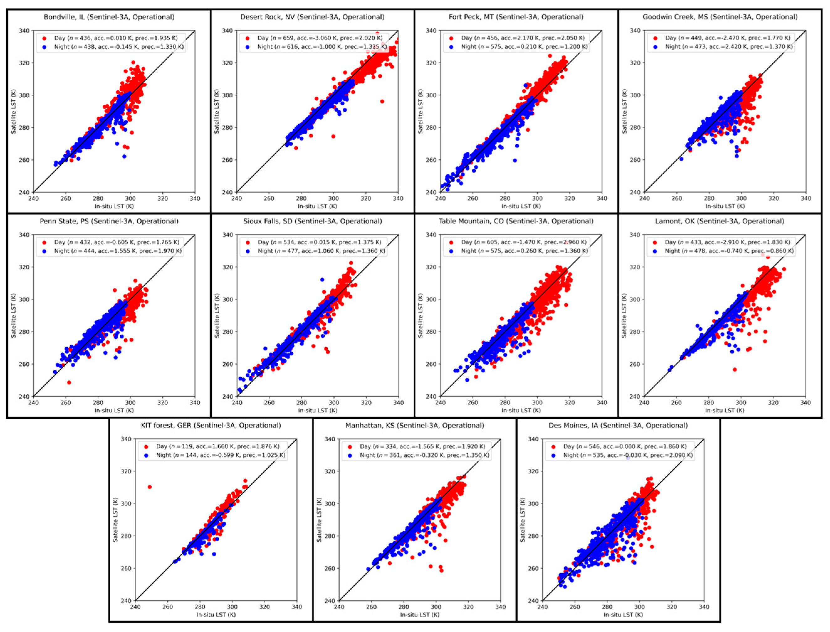
3.1. Validation of SL_2_LST Products

In general, for the SL_2_LST products of both SLSTR-A and SLSTR-B, the differences with respect to the in situ measurements from the eleven stations are clustered around the 1:1 line. From both Figure 7 and Figure 8 and

Table 5. Daytime and night-time in situ validation statistics for the SL_2_LST product for SLSTR-A and SLSTR-B, where N are the number of clear-sky matchups, Acc. is the accuracy, and Prec. is the precision.

Site	S3A						S3B
	Day			Night			Day			Night
	N	Acc.	Prec.	N	Acc.	Prec.	N	Acc.	Prec.	N	Acc.	Prec.
Bondville, IL, USA	436	0.01	1.93	438	−0.14	1.33	364	0.00	2.16	382	−0.27	1.23
Desert Rock, NV, USA	659	−3.06	2.02	616	−1.00	1.32	534	−2.79	1.73	567	−1.46	1.38
Fort Peck, MT, USA	456	2.17	2.05	575	0.21	1.20	396	1.98	1.89	483	−0.07	1.39
Goodwin Creek, MS, USA	449	−2.47	1.77	473	2.42	1.37	393	−2.49	1.61	419	1.97	1.36
Des Moines, IA, USA	546	0.00	1.86	535	−0.03	2.09	520	0.00	1.49	476	−0.49	1.76
KIT Forest, Germany	119	1.66	1.87	144	−0.59	1.02	118	1.00	1.62	140	−0.40	0.86
Manhattan, KS, USA	334	−1.56	1.92	361	−0.32	1.35	348	−1.13	1.57	356	−0.33	1.17
Penn State University, University Park, PA, USA	432	−0.60	1.76	444	1.55	1.97	358	−0.81	1.35	374	1.54	2.03
Southern Great Plains, OK, USA	433	−2.91	1.83	478	−0.74	0.86	382	−2.87	1.91	433	−0.85	0.92
Sioux Falls, SD, USA	534	0.01	1.37	477	1.06	1.36	465	0.13	1.55	452	1.03	1.35
Table Mountain, CO, USA	605	−1.47	2.96	575	0.26	1.36	555	−1.03	2.76	536	−0.04	1.46

, we can conclude that the performance of the SL_2_LST product is consistent between SLSTR-A and SLSTR-B. While no common systematic positive or negative difference is present across all the stations, the validation for some stations exhibits larger differences. At these stations, the larger differences occur for both SLSTR-A and SLSTR-B, indicating that the implementation of both the retrieval algorithm and the cloud masking scheme is consistent for both sensors.

Several outliers are present in the validation at each station. These could be due to lower quality in situ data for the matchup or the retrieval algorithm not sufficiently representing an extreme condition. A greater clustering of outliers at some of the stations is clearly visible below the 1:1 line and is evidence of failures in the cloud detection scheme. This is particularly noticeable for the Goodwin Creek site, with a large number of matchups below the 1:1 line.

There is insufficient evidence to suggest the differences across the stations have a systematic dependence on temperature, though this is an area for more investigation. An exception might appear to be at the Bondville site, where there is an upward curve to the matchups at higher temperatures. Previous studies [36] have also found similar results at higher temperatures, and they concluded these were a result of the change in surface type during and after the harvest of the crops of the land surrounding the instrumented site.

Table 5 shows the night-time differences for the SL_2_LST product are in general smaller than the daytime differences with the corresponding standard deviations also lower. This is in line with expectations and is due primarily to the influence of solar radiation during daytime with the satellite sensors observing different proportions of sunlit and shadow areas within their field of view. For the most part, these corresponding proportions are not represented within the field of view of the in situ sensors. Furthermore, Table 5 shows that the magnitude of the differences can vary considerably between different stations. For instance, for Bondville and Sioux Falls, the difference is near-zero, while at other sites such as Desert Rock and Southern Great Plains, the validation shows larger negative differences. Where larger differences are found these are for the most part negative, being influenced by failures in the cloud masking. Individual sites where large negative differences are found were assessed matchup-by-matchup over a wider 51 × 51 grid to identify these cloud failures. The number of matchups is higher for SLSTR-A than for SLSTR-B, which is expected since the operational product for SLSTR-B was not released until November of 2018, whereas we include matchups from the whole of 2018 for SLSTR-A.

Overall, the differences for both SLSTR-A and SLSTR-B range between approximately ±2.5 K for daytime and ±1.5 K for night-time. The standard deviations range generally between 0 and 2 K, with daytime larger than night-time. An outlier here is the Table Mountain station, which has larger daytime standard deviations of 2.96 K (SLSTR-A) and 2.76 (SLSTR-B). This station is situated in a valley and is surrounded by mountains, with a larger seasonal cycle that is possibly due to different proportions of sun and shadow throughout the year [36]. The mean absolute differences across the stations are 1.45 K (daytime) and 0.76 K (night-time) for SLSTR-A, and 1.29 K (daytime) and 0.77 K (night-time) for SLSTR-B.

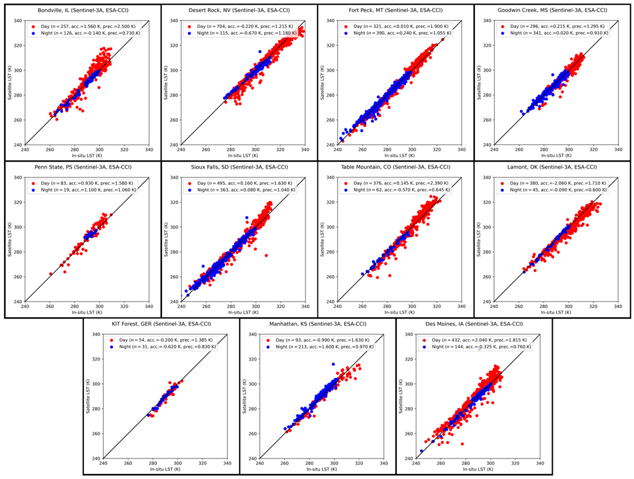
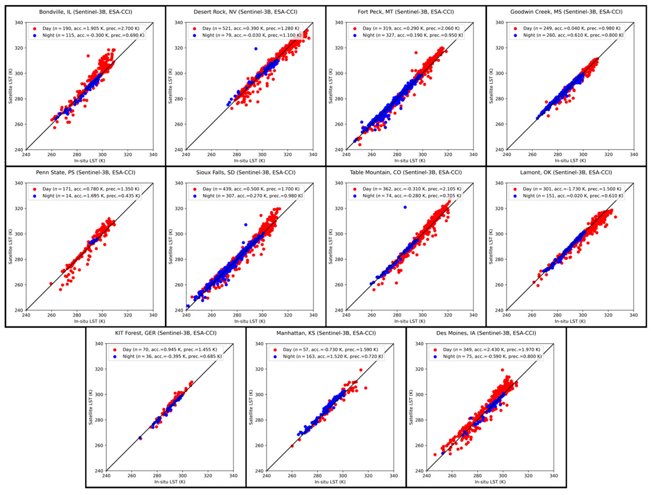
3.2. Validation of LST_cci Products

The results for the LST_cci SLSTR products are shown in Figure 9 and Figure 10, with the statistics presented in

Table 6. Daytime and night-time in situ validation statistics for the LST_cci product for SLSTR-A and SLSTR-B, where N are the number of clear-sky matchups, Acc. is the accuracy, and Prec. is the precision.

Site	S3A						S3B
	Day			Night			Day			Night
	N	Acc.	Prec.	N	Acc.	Prec.	N	Acc.	Prec.	N	Acc.	Prec.
Bondville, IL, USA	257	1.56	2.50	126	−0.14	0.73	190	1.90	2.70	115	−0.30	0.69
Desert Rock, NV, USA	704	−0.22	1.22	115	−0.67	1.18	521	0.39	1.28	79	−0.03	1.10
Fort Peck, MT, USA	321	0.01	1.90	390	0.24	1.05	319	0.29	2.06	327	0.19	0.95
Goodwin Creek, MS, USA	296	0.21	1.29	341	0.02	0.91	249	0.04	0.98	260	0.61	0.80
Des Moines, IA, USA	432	2.04	1.82	144	−0.33	0.76	349	2.43	1.97	75	−0.59	0.80
KIT Forest, Germany	54	−0.20	1.38	31	−0.62	0.83	70	0.94	1.45	36	−0.39	0.68
Manhattan, KS, USA	93	−0.99	1.63	213	1.60	0.97	57	−0.73	1.59	163	1.52	0.72
Penn State University, University Park, PA, USA	83	0.93	1.58	19	1.10	1.06	171	0.78	1.35	14	1.69	0.43
Southern Great Plains, OK, USA	380	−2.06	1.71	45	−0.09	0.60	301	−1.73	1.50	151	0.02	0.61
Sioux Falls, SD, USA	495	0.16	1.63	363	0.08	1.04	439	0.50	1.70	307	0.27	0.98
Table Mountain, CO, USA	376	0.14	2.39	62	−0.57	0.64	362	−0.31	2.10	74	−0.28	0.70

. As for the SL_2_LST products, the differences with respect to the in situ measurements for the LST_cci SLSTR-A and SLSTR-B products from the eleven stations are also clustered around the 1:1 line. The performance of the LST_cci products is, therefore, consistent between SLSTR-A and SLSTR-B. The validation indicates an improvement with the LST_cci products compared with their corresponding SL_2_LST products. The mean absolute differences across the stations from Table 6 for the LST_cci products are 0.77 K (daytime) and 0.50 K (night-time) for SLSTR-A, and 0.91 K (daytime) and 0.54 K (night-time) for SLSTR-B. The standard deviations mostly range between 0 and 2 K for daytime and generally within 1 K at night-time, which is lower than for the SL_2_LST products. There is consistency here with the range of values for the pixel-by-pixel product uncertainty, which is generally between 0 and 2 K, as highlighted in Figure 3. An exception is for Bondville, which has a high standard deviation during the daytime for both sensors, though as explained previously, this site is more heterogeneous than the majority of the other sites.

A noticeable difference between the validation of the SL_2_LST products and the LST_cci products is in the number of matchups. These are considerably fewer for the LST_cci products, particularly for night-time. As such, many of the negative outliers in the validation have been removed, as seen in Figure 9 and Figure 10. This is partly responsible for reducing the standard deviations of the LST_cci products. This much-improved hit rate (correctly identified cloudy pixels) of the cloud masking is, however, countered to some extent by what appears to be an increase in the false alarm rate (incorrectly masked clear pixels). The hit rate has improved for both day and night for both sensors, but the false alarm rate has increased substantially during the night.

The differences for nearly all sites are lower for LST_cci than for SL_2_LST, although there are some exceptions, such as Bondville during the daytime and Manhattan during the night-time. For Bondville, the removal of many of the negative outliers due to better cloud clearing has resulted in an overall positive difference. This is in line with results from other studies [36], which show a positive bias for satellite LST with respect to the in situ LST, particularly during the summer. For Manhattan, the retrieval algorithm for night-time seems to produce a small but noticeable positive difference for both LST_cci SLSTR-A and SLSTR-B. The likelihood here is that the retrieval coefficient does not adequately represent the emissivity of the site.

4. Discussion

In this paper, we show the validation results over eleven well-established in situ sites for LST, which have been used in multiple previous studies. Larger differences overall with respect to the in situ measurements are seen for the operational SL_2_LST SLSTR products than for their corresponding LST_cci SLSTR products. The reasons for these differences vary between stations and can be influenced by surface heterogeneity around the station, in both space and time or from differences in the products. Differences with respect to in situ measurements where a station is heterogeneous over time have been reported elsewhere for the SL_2_LST SLSTR products [44]. It is clear that the improvements made in the implementation of the retrieval algorithm have reduced the differences between the LST_cci products and the ground-based observations. However, a greater impact appears to have been made by reducing the number of failures in the cloud detection scheme.

The improvements in the LST_cci implementation, which include the generation of retrieval coefficients, and higher stratification of the auxiliary data for the biome and fractional vegetation, have resulted in better validation statistics and thus greater confidence in the products. It is expected that the climate quality LST_cci would show improved validation results, and, indeed, this is consistent with the findings of a previous assessment of the LST_cci products [79]. Since the retrieval algorithm is biome based with separate coefficients for each biome–diurnal combination, the improved validation results, which are evident for most of the sites, imply an improvement for multiple coefficients. This is largely due to a database of reference states which better captures the global variation in surface and atmospheric conditions, but dynamic fractional vegetation data as a proxy for the surface emissivity will also likely be a causal factor in the improved performance for LST_cci compared with the climatological approach for SL_2_LST. For sites with more variable atmospheric conditions, a better representation of the water vapour auxiliary data will elicit improvements. Accounting for the annual change in biome for LST_cci also presents more applicable coefficients compared with a static biome classification for SL_2_LST which dates back to 2006.

The cloud masking has a clear influence on the validation results. Whilst satellite pixels are cloud-masked for clear-sky-only matchups prior to the validation, poor cloud masking can miss cloud-contaminated pixels, thus impacting the validation. For the SL_2_LST products, the clustering of many matchups below the 1:1 line, along with several larger outliers, is evidence that the cloud masking scheme is not performing optimally. This is a clear shortcoming of the current SL_2_LST implementation. In contrast, the cloud masking has removed most of these outliers in the LST_cci products and reduced clustering below the 1:1 line, although the false alarm rate has also increased. While the validation results are not a direct verification of the cloud masks for the different products, they do provide strong evidence of their performance.

The validation presented here displays similar tendencies with respect to the station-by-station analysis to previous studies, which have utilised some of the same in situ sites [36,39]. These studies also found larger differences for certain stations, such as Bondville and Desert Rock, as a result of surface heterogeneity on the scale of the satellite pixel not being adequately represented within the field of view of the in situ radiometers. Nonetheless, valuable insights are still made by including such sites, particularly for retrieval algorithms, which have separate coefficients based on land cover, as is the case for the SLSTR algorithm presented here, since it provides data for assessment over land covers that may not otherwise be validated. Future investigation could assess the validation results with respect to other factors which affect the accuracy of satellite-derived LST. These include viewing geometry differences between the in situ sensor and the satellite pixel; upscaling of the in situ field of view to the footprint of the overstriking pixel, and any differences in orography; coincident atmospheric conditions; and calibration of the respective in situ radiometers.

The accuracies of the SLSTR products presented here are comparable to those reported for other common LST products in previous validation studies. For instance, the MOD11A1 and MYD11A1 LST products from MODIS have been well validated against in situ observations with accuracies of near 1 K [80,81,82]. For the Visible Infrared Imaging Radiometer Suite (VIIRS), accuracies are also reported to be around 1 K [74,83]. For other common LST products, such as The Spinning Enhanced Visible and InfraRed Imager (SEVIRI) on Meteosat Second Generation and the Advanced Very High-Resolution Radiometer (AVHRR) on Metop, the accuracies reported are also similar to our study [84]. A previous intercomparison between the SL_2_LST product and operational MODIS MOD11A1 indicates good agreement [21].

Even though we see clear improvements in the LST_cci SLSTR products compared to the operational SL_2_LST products, there remain improvements still to be made. Firstly, the validation results still show larger differences at some sites, such as Bondville and Southern Great Plains (daytime) and Manhattan (night-time). Some of these are due to larger heterogeneity at the sites as these are often not represented in the field of view of the ground-based radiometers, while for others it may be that the database of reference states is not adequately representing the surface conditions for every biome. Revisiting the database to ensure it captures the typical global surface and atmospheric conditions for each biome, but also the realistic extremes, is recommended. Secondly, the cloud masking would seem to be too strict for the night-time retrievals, and at certain sites during the daytime. Each biome–diurnal combination is represented by a different set of cloud coefficients to represent the histogram of expected brightness temperatures and their differences. The larger false alarm rate at some stations suggests this histogram is too narrow for these biomes at night and further research is required to fine-tune these histograms.

Beyond these potential improvements, there are some limitations with the products as a result of the choice of retrieval algorithm. First, emissivity is not explicit but rather dependent on a combination of biome and fractional vegetation cover. However, the sub-division of bare soil into different principal soil types does better capture the variability in the emissivity where the fraction vegetation cover is zero. Second, emissivity may vary by latitude within a biome, with some individual biomes, for instance, occurring across high, mid, and low latitudes. Numerous studies have proposed alternative algorithms for SLSTR [41,42,43,44,85]. However, despite the limitations in the current implementation, a recent algorithm intercomparison study of several operation algorithms [22] concluded the algorithm used here is the optimal choice for ATSR/SLSTR, as the increased resolution in coefficient space can better represent the true surface and atmospheric states resulting in low global biases. The algorithm itself is particularly suited to instruments with low radiometric noise, as demonstrated in [22]. Third, the products do not take into account the impact on LST retrievals from high aerosol load. For Sea Surface Temperature, tropospheric mineral dust aerosol can cause biases of several tenths of a degree [86,87]. Nonetheless, the ATSR/SLSTR algorithm has been implemented in the LST_cci for both the SLSTRs and AATSR, and the latter product was included in a stability and trends analysis [88] with the conclusion that this dataset was free from non-climatic discontinuities and suitable for climate trend analysis.

Evolutions of the algorithm could include latitudinal dependent coefficients for each biome and a correction for the impact of dust aerosol optical depth. Other potential improvements could arise from the use of temperature-dependent coefficients, which could minimise any higher biases at warm daytime temperatures, as can be seen for Bondville, Sioux Falls, Des Moines, and Table Mountain during the summer months. Finally, better stratification of the soil, rock, and urban biomes could facilitate more representative coefficients for these surfaces where the emissivity can have a larger variation.

Future work in LST_cci is already underway to improve the cloud masking for the SLSTR products. Rather than using ERA-Interim profile data, which consequently finish in 2019, these are being replaced by ERA5 profile data [52] to exploit the increased temporal resolution. The rationale is that temporal interpolation between 1-hourly data from ERA5 will be better suited to generating expected brightness temperatures and their differences compared with temporal interpolation between 6-hourly data from ERA-Interim. Together with the other improvements detailed in this paper for the LST_cci products, recommendations can be made to mission management for evolutions to the SLSTR operational product to ensure it can meet mission requirements on accuracy.

5. Conclusions

This paper presents the first detailed description of two publicly released data products for SLSTR, and their validation: the operational SL_2_LST product; and the LST_cci product. Both these products utilise the same functional form of the retrieval algorithm [12] but differ in their implementation. Several evolutions have been made in the LST_cci product compared with the SL_2_LST product. These include (i) an improved database of reference states utilising the latest profile and emissivity data; (ii) dynamic auxiliary data for fractional vegetation; (iii) dynamic biome data with increased stratification of the classification; and (iv) improvements in the cloud detection scheme.

The evaluation of the respective SLSTR products is by way of validation against ground-based observations from eleven well-established in situ stations. LST differences with respect to the in situ measurements and the corresponding standard deviations are presented in the form of accuracy and precision to enable a direct comparison with climate change and mission requirements. The validation results presented here indicate that both the SL_2_LST and LST_cci products for both SLSTR-A and SLSTR-B sensors meet the 1 K accuracy requirements, for the SLSTR mission and from GCOS, for night-time. Moreover, the LST_cci products sensors also meet the daytime accuracy requirements, whereas the SL_2_LST products are slightly higher than this 1 K requirement during the day. For precision, which is only stated by GCOS for climate products, the LST_cci on average meets this 1 K requirement at night-time but is slightly above this during the day. Continued improvements to the in situ reference stations are needed including better methods to compute the in situ LST of the satellite footprint.

Based on the results shown here, the LST_cci products are an improvement on the operational SL_2_LST products, and meet, or are very close to, the GCOS requirements, suggesting they are of sufficient quality for use in climate studies. Implementation of the enhanced features used in the development of the LST_cci products would be recommended for the operational SL_2_LST products to ensure they fully meet mission requirements. We recommend the use of the LST_cci products for climate studies, with the SL_2_LST products designed for applications requiring near-real-time data.

References

1. Sellers, P.J.; Dickinson, R.E.; Randall, D.A.; Betts, A.K.; Hall, F.G.; Berry, J.A.; Collatz, G.J.; Denning, A.S.; Mooney, H.A.; Nobre, C.A.; et al. Modeling the exchanges of energy, water, and carbon between continents and the atmosphere. Science 1997, 275, 502–509. [Google Scholar] [CrossRef] [PubMed]
2. Sun, J.; Mahrt, L. Determination of surface fluxes from the surface radiative temperature. J. Atmos. Sci. 1995, 52, 1096–1106. [Google Scholar] [CrossRef]
3. Norman, J.M.; Becker, F. Terminology in thermal infrared remote sensing of natural surfaces. Agric. For. Meteorol. 1995, 77, 153–166. [Google Scholar] [CrossRef]
4. Schaadlich, S.; Gottsche, F.M.; Olesen, F.S. Influence of land parameters and atmosphere on Meteosat brightness temperatures and generation of land surface temperature maps by temporally and spatially interpolating atmospheric correction. Remote Sens. Environ. 2001, 75, 39–46. [Google Scholar] [CrossRef]
5. Dash, P.; Gottsche, F.M.; Olesen, F.S.; Fischer, H. Land surface temperature and emissivity estimation from passive sensor data: Theory and practice—Current trends. Int. J. Remote Sens. 2002, 23, 2563–2594. [Google Scholar] [CrossRef]
6. Lillesand, T.M.; Kiefer, R.W. Remote Sensing and Image Interpretation; Wiley: New York, NY, USA, 1987. [Google Scholar]
7. Becker, F.; Li, Z.L. Towards a local split window method over land surfaces. Int. J. Remote Sens. 1990, 11, 369–393. [Google Scholar] [CrossRef]
8. Wan, Z.; Dozier, J. A generalized split-window algorithm for retrieving land surface temperature from space. IEEE Trans. Geosci. Remote Sens. 1996, 34, 892–905. [Google Scholar]
9. Prata, A.J. Land-surface temperatures derived from the Advanced Very High-Resolution Radiometer and the Along-Track Scanning Radiometer. 1. Theory. J. Geophys. Res.-Atmos. 1993, 98, 16689–16702. [Google Scholar] [CrossRef]
10. Prata, A.J. Land-surface temperatures derived from the Advanced Very High-Resolution Radiometer and the Along-Track Scanning Radiometer. 2. Experimental results and validation of AVHRR algorithms. J. Geophys. Res.-Atmos. 1994, 99, 13025–13058. [Google Scholar] [CrossRef]
11. Prata, F. Land Surface Temperature Measurement from Space: AATSR Algorithm Theoretical Basis Document; CSIRO: Aspendale, Australia, 2002.
12. Ghent, D.J.; Corlett, G.K.; Göttsche, F.M.; Remedios, J.J. Global Land Surface Temperature from the Along-Track Scanning Radiometers. J. Geophys. Res. Atmos. 2017, 122, 12167–12193. [Google Scholar] [CrossRef]
13. Trigo, I.F.; Peres, L.F.; DaCamara, C.C.; Freitas, S.C. Thermal land surface emissivity retrieved from SEVIRI/meteosat. IEEE Trans. Geosci. Remote Sens. 2008, 46, 307–315. [Google Scholar] [CrossRef]
14. Sobrino, J.A.; Raissouni, N. Toward remote sensing methods for land cover dynamic monitoring: Application to Morocco. Int. J. Remote Sens. 2000, 21, 353–366. [Google Scholar] [CrossRef]
15. Sobrino, J.A.; El-Kharraz, J.; Li, Z.-L. Surface temperature and water vapour retrieval from MODIS data. Int. J. Remote Sens. 2003, 24, 5161–5182. [Google Scholar] [CrossRef]
16. Jiménez-Muñoz, J.C.; Sobrino, J.A. A generalized single-channel method for retrieving land surface temperature from remote sensing data. J. Geophys. Res. 2003, 108, 4688. [Google Scholar] [CrossRef]
17. Jiménez-Muñoz, J.C.; Cristobal, J.; Sobrino, J.A.; Soria, G.; Ninyerola, M.; Pons, X. Revision of the single-channel algorithm for land surface temperature retrieval from Landsat thermal-infrared data. IEEE Trans. Geosci. Remote Sens. 2009, 47, 339–349. [Google Scholar] [CrossRef]
18. Gillespie, A.; Rokugawa, S.; Matsunaga, T.; Cothern, J.S.; Hook, S.; Kahle, A.B. A temperature and emissivity separation algorithm for advanced spaceborne thermal emission and reflection radiometer (ASTER) images. IEEE Trans. Geosci. Remote Sens. 1998, 36, 1113–1126. [Google Scholar] [CrossRef]
19. Hulley, G.C.; Hook, S.J. Generating consistent land surface temperature and emissivity products between ASTER and MODIS data for Earth science research. IEEE Trans. Geosci. Remote Sens. 2011, 49, 1304–1315. [Google Scholar] [CrossRef]
20. Wan, Z.; Li, Z.-L. A physics-based algorithm for retrieving land-surface emissivity and temperature from EOS/MODIS data. IEEE Trans. Geosci. Remote Sens. 1997, 35, 980–996. [Google Scholar]
21. Li, Z.-L.; H Wu, S.-B.; Duan, W.; Zhao, H.; Ren, X.; Liu, P.; Leng, R.; Tang, X.; Ye, J.; Zhu, Y.; et al. Satellite Remote Sensing of Global Land Surface Temperature: Definition, Methods, Products, and Applications. Rev. Geophys. 2023, 61, e2022RG000777. [Google Scholar] [CrossRef]
22. Perry, M.; Ghent, D.; Jimenez, C.; Dodd, E.; Ermida, S.; Trigo, I.F.; Veal, K. Multi-Sensor thermal infrared and microwave land surface temperature algorithm intercomparison. Remote Sens. 2020, 12, 4164. [Google Scholar] [CrossRef]
23. Donlon, C.; Berruti, B.; Buongiorno, A.; Ferreira, M.-H.; Féménias, P.; Frerick, J.; Goryl, P.; Klein, U.; Laur, H.; Mavrocordatos, C.; et al. The Global Monitoring for Environment and Security (GMES) Sentinel-3 mission. Remote Sens. Environ. 2012, 120, 37–57. [Google Scholar] [CrossRef]
24. Llewellyn-Jones, D.; Remedios, J. The Advanced Along Track Scanning Radiometer (AATSR) and its predecessors ATSR-1 and ATSR-2: An introduction to the special issue. Remote Sens. Environ. 2012, 116, 1–3. [Google Scholar] [CrossRef]
25. Smith, D.; Hunt, S.E.; Etxaluze, M.; Peters, D.; Nightingale, T.; Mittaz, J.; Woolliams, E.R.; Polehampton, E. Traceability of the Sentinel-3 SLSTR Level-1 Infrared Radiometric Processing. Remote Sens. 2021, 13, 374. [Google Scholar] [CrossRef]
26. Merchant, C.J.; Embury, O.; Roberts-Jones, J.; Fiedler, E.; Bulgin, C.E.; Corlett, G.K.; Good, S.; McLaren, A.; Rayner, N.; Morak-Bozzo, S.; et al. Sea surface temperature datasets for climate applications from Phase 1 of the European Space Agency Climate Change Initiative (SST CCI). Geosci. Data J. 2014, 1, 179–191. [Google Scholar] [CrossRef]
27. Wan, Z.; Zhang, Y.; Zhang, Y.Q.; Li, Z.L. Validation of the land-surface temperature products retrieved from Terra Moderate Resolution Imaging Spectroradiometer data. Remote Sens. Environ. 2002, 83, 163–180. [Google Scholar] [CrossRef]
28. Gottsche, F.M.; Olesen, F.S.; Bork-Unkelbach, A. Validation of land surface temperature derived from MSG/SEVIRI with in situ measurements at Gobabeb, Namibia. Int. J. Remote Sens. 2013, 34, 3069–3083. [Google Scholar] [CrossRef]
29. Barreto, A.; Arbelo, M.; Hernandez-Leal, P.A.; Nunez-Casillas, L.; Mira, M.; Coll, C. Evaluation of Surface Temperature and Emissivity Derived from ASTER Data: A Case Study Using Ground-Based Measurements at a Volcanic Site. J. Atmos. Ocean. Technol. 2010, 27, 1677–1688. [Google Scholar] [CrossRef]
30. Coll, C.; Caselles, V.; Galve, J.M.; Valor, E.; Niclos, R.; Sanchez, J.M.; Rivas, R. Ground measurements for the validation of land surface temperatures derived from AATSR and MODIS data. Remote Sens. Environ. 2005, 97, 288–300. [Google Scholar] [CrossRef]
31. Coll, C.; Wan, Z.M.; Galve, J.M. Temperature-based and radiance-based validations of the V5 MODIS land surface temperature product. J. Geophys. Res.-Atmos. 2009, 114, D20102. [Google Scholar] [CrossRef]
32. Göttsche, F.M.; Olesen, F.; Trigo, I.; Bork-Unkelbach, A.; Martin, M. Long Term Validation of Land Surface Temperature Retrieved from MSG/SEVIRI with Continuous in-Situ Measurements in Africa. Remote Sens. 2016, 8, 410. [Google Scholar] [CrossRef]
33. Hulley, G.C.; Malakar, N.K.; Islam, T.; Freepartner, R.J. NASA’s MODIS and VIIRS Land Surface Temperature and Emissivity Products: A Long-Term and Consistent Earth System Data Record. IEEE J. Sel. Top. Appl. Earth Obs. Remote Sens. 2018, 11, 522–535. [Google Scholar] [CrossRef]
34. Hulley, G.C.; Gottsche, F.M.; Rivera, G.; Hook, S.J.; Freepartner, R.J.; Martin, M.A.; Cawse-Nicholson, K.; Johnson, W.R. Validation and Quality Assessment of the ECOSTRESS Level-2 Land Surface Temperature and Emissivity Product. IEEE Trans. Geosci. Remote Sens. 2021, 60, 5000523. [Google Scholar] [CrossRef]
35. Niclos, R.; Galve, J.M.; Valiente, J.A.; Estrela, M.J.; Coll, C. Accuracy assessment of land surface temperature retrievals from MSG2-SEVIRI data. Remote Sens. Environ. 2011, 115, 2126–2140. [Google Scholar] [CrossRef]
36. Martin, M.A.; Ghent, D.; Pires, A.C.; Göttsche, F.-M.; Cermak, J.; Remedios, J.J. Comprehensive In Situ Validation of Five Satellite Land Surface Temperature Data Sets over Multiple Stations and Years. Remote Sens. 2019, 11, 479. [Google Scholar] [CrossRef]
37. Li, S.; Yu, Y.; Sun, D.; Tarpley, D.; Zhan, X.; Chiu, L. Evaluation of 10 year AQUA/MODIS land surface temperature with SURFRAD observations. Int. J. Remote Sens. 2014, 35, 830–856. [Google Scholar] [CrossRef]
38. Ouyang, X.; Chen, D.; Duan, S.-B.; Lei, Y.; Dou, Y.; Hu, G. Validation and Analysis of Long-Term AATSR Land Surface Temperature Product in the Heihe River Basin, China. Remote Sens. 2017, 9, 152. [Google Scholar] [CrossRef]
39. Yu, Y.; Tarpley, D.; Privette, J.L.; Flynn, L.E.; Xu, H.; Chen, M.; Vinnikov, K.Y.; Sun, D.; Tian, Y. Validation of GOES-R Satellite Land Surface Temperature Algorithm Using SURFRAD Ground Measurements and Statistical Estimates of Error Properties. IEEE Trans. Geosci. Remote Sens. 2012, 50, 704–713. [Google Scholar] [CrossRef]
40. Wang, K.; Liang, S. Evaluation of aster and modis land surface temperature and emissivity products using long-term surface longwave radiation observations at surfrad sites. Remote Sens. Environ. 2009, 113, 1556–1565. [Google Scholar] [CrossRef]
41. Zhang, S.; Duan, S.-B.; Li, Z.-L.; Huang, C.; Wu, H.; Han, X.-J.; Leng, P.; Gao, M. Improvement of Split-Window Algorithm for Land Surface Temperature Retrieval from Sentinel-3A SLSTR Data Over Barren Surfaces Using ASTER GED Product. Remote Sens. 2019, 11, 3025. [Google Scholar] [CrossRef]
42. Zheng, Y.; Ren, H.; Guo, J.; Ghent, D.; Tansey, K.; Hu, X.; Nie, J.; Chen, S. Land Surface Temperature Retrieval from Sentinel-3A Sea and Land Surface Temperature Radiometer, Using a Split-Window Algorithm. Remote Sens. 2019, 11, 650. [Google Scholar] [CrossRef]
43. Yang, J.; Zhou, J.; Göttsche, F.-M.; Long, Z.; Ma, J.; Luo, R. Investigation and validation of algorithms for estimating land surface temperature from Sentinel-3 SLSTR data. Int. J. Appl. Earth Obs. Geoinf. 2020, 91, 102136. [Google Scholar] [CrossRef]
44. Pérez-Planells, L.; Niclòs, R.; Puchades, J.; Coll, C.; Göttsche, F.-M.; Valiente, J.A.; Valor, E.; Galve, J.M. Validation of Sentinel-3 SLSTR Land Surface Temperature Retrieved by the Operational Product and Comparison with Explicitly Emissivity-Dependent Algorithms. Remote Sens. 2021, 13, 2228. [Google Scholar] [CrossRef]
45. Merchant, C.J.; Matthiesen, S.; Rayner, N.A.; Remedios, J.J.; Jones, P.D.; Olesen, F.; Trewin, B.; Thorne, P.W.; Auchmann, R.; Corlett, G.K.; et al. The surface temperatures of Earth: Steps towards integrated understanding of variability and change. Geosci. Instrum. Methods Data Syst. 2013, 2, 305–321. [Google Scholar] [CrossRef]
46. Ghent, D.; Remedios, J.; Dodd, E. Sentinel-3 Optical Products and Algorithm Definition: Land Surface Temperature. Reference: S3-L2-SD-03-T03-ULNILU-ATBD_L2LST, Version 4.0. 2021. Available online: https://sentinels.copernicus.eu/documents/247904/349589/S3-L2-SD-03-T03-ULNILU-ATBD-L2LST_v4.0.pdf/4ddf3000-59f9-383f-bfcc-753a3820acd1?t=1683480828288 (accessed on 20 May 2024).
47. Hocking, J.; Rayer, P.; Rundle, D.; Saunders, R.; Matricardi, M.; Geer, A. RTTOV v12 Users Guide; NWPSAF-MO-UD-037 v1.3; EUMETSAT NWP-SAF: Lannion, France, 2019. [Google Scholar]
48. Saunders, R.; Hocking, J.; Rundle, D.; Rayer, P.; Havemann, S.; Matricardi, M.; Geer, A.; Lupu, C.; Brunel, P.; Vidot, J. RTTOV-12 Science and Validation Report; NWPSAF-MO-TV-41 v1.0; EUMETSAT NWP-SAF: Lannion, France, 2017. [Google Scholar]
49. Ermida, S.L.; Trigo, I.F. A Comprehensive Clear-Sky Database for the Development of Land Surface Temperature Algorithms. Remote Sens. 2022, 14, 2329. [Google Scholar] [CrossRef]
50. Dee, D.P.; Uppala, S.M.; Simmons, A.J.; Berrisford, P.; Poli, P.; Kobayashi, S.; Rae, U.; Balmaseda, M.A.; Balsamo, G.; Bauer, P.; et al. The ERA-Interim reanalysis: Configuration and performance of the data assimilation system. Q. J. R. Meteorol. Soc. 2011, 137, 553–597. [Google Scholar] [CrossRef]
51. Seemann, S.W.; Borbas, E.E.; Knuteson, R.O.; Stephenson, G.R.; Huang, H.-L. Development of a global infrared land surface emissivity database for application to clear sky sounding retrievals from multispectral satellite radiance measurements. J. Appl. Meteorol. Climatol. 2008, 47, 108–123. [Google Scholar] [CrossRef]
52. Hersbach, H.; Bell, B.; Berrisford, P.; Hirahara, S.; Horányi, A.; Muñoz-Sabater, J.; Nicolas, J.; Peubey, C.; Radu, R.; Schepers, D.; et al. The ERA5 global reanalysis. Q. J. R. Meteorol. Soc. 2020, 146, 1999–2049. [Google Scholar] [CrossRef]
53. Borbas, E.E.; Hulley, G.; Feltz, M.; Knuteson, R.; Hook, S. The Combined ASTER MODIS Emissivity over Land (CAMEL) Part 1: Methodology and High Spectral Resolution Application. Remote Sens. 2018, 10, 643. [Google Scholar] [CrossRef]
54. Feltz, M.; Borbas, E.; Knuteson, R.; Hulley, G.; Hook, S. The Combined ASTER MODIS Emissivity over Land (CAMEL) Part 2: Uncertainty and Validation. Remote Sens. 2018, 10, 664. [Google Scholar] [CrossRef]
55. Arino, O.; Gross, D.; Ranera, F.; Leroy, M.; Bicheron, P.; Brockman, C.; Defourny, P.; Vancutsem, C.; Achard, F.; Durieux, L.; et al. GlobCover: ESA Service for Global Land Cover from MERIS; IEEE: New York, NY, USA, 2007. [Google Scholar]
56. ESA. Land Cover CCI Product User Guide Version 2. Tech. Rep. 2017. Available online: https://maps.elie.ucl.ac.be/CCI/viewer/download/ESACCI-LC-Ph2-PUGv2_2.0.pdf (accessed on 8 May 2024).
57. Baret, F.; Weiss, M.; Lacaze, R.; Camacho, F.; Makhmara, H.; Pacholcyzk, P.; Smets, B. GEOV1: LAI and FAPAR essential climate variables and FCOVER global time series capitalizing over existing products. Part1: Principles of development and production. Remote Sens. Environ. 2013, 137, 299–309. [Google Scholar] [CrossRef]
58. US National Ice Center. IMS Daily Northern Hemisphere Snow and Ice Analysis at 1 km, 4 km, and 24 km Resolutions, Version 1 [Data Set]; National Snow and Ice Data Center: Boulder, CO, USA, 2008. [Google Scholar] [CrossRef]
59. Bulgin, C.E.; Sembhi, H.; Ghent, D.; Remedios, J.; Merchant, C.J. Cloud Clearing Techniques over Land for Land Surface Temperature Retrieval from the Advanced Along Track Scanning Radiometer. Int. J. Remote Sens. 2014, 35, 3594–3615. [Google Scholar] [CrossRef]
60. Ghent, D.; Veal, K.; Trent, T.; Dodd, E.; Sembhi, H.; Remedios, J. A New Approach to Defining Uncertainties for MODIS Land Surface Temperature. Remote Sens. 2019, 11, 1021. [Google Scholar] [CrossRef]
61. Bulgin, C.E.; Embury, O.; Corlett, G.; Merchant, C.J. Independent uncertainty estimates for coefficient based sea surface temperature retrieval from the Along-Track Scanning Radiometer instruments. Remote Sens. Environ. 2016, 178, 213–222. [Google Scholar] [CrossRef]
62. Merchant, C.J.; Holl, G.; Mittaz, J.P.D.; Wooliams, E.R. Radiance Uncertainty Characterisation to Facilitate Climate Data Record Creation. Remote Sens. 2019, 11, 474. [Google Scholar] [CrossRef]
63. Bulgin, C.E.; Ermida, S.; Jimenez, C.; Veal, K.; Ghent, D. Land Surface Temperature CCI: End-To-End ECV Uncertainty Budget. Reference: LST-CCI-D2.3-E3UB Version 3.0. 2023. Available online: https://admin.climate.esa.int/media/documents/LST-CCI-D2.3-E3UB_-_i3r0_-_End-to-End_ECV_Uncertainty_Budget.pdf (accessed on 22 May 2024).
64. Camacho, F.; Cernicharo, J.; Lacaze, R.; Baret, F.; Weiss, M. GEOV1: LAI, FAPAR essential climate variables and FCOVER global time series capitalizing over existing products. Part 2: Validation and intercomparison with reference products. Remote Sens. Environ. 2013, 137, 310–329. [Google Scholar] [CrossRef]
65. Polehampton, E.; Cox, C.; Smith, D.; Ghent, D.; Wooster, M.; Xu, W.; Bruniquel, J.; Henocq, C.; Dransfeld, S. Copernicus Sentinel-3 SLSTR Land User Handbook. Reference: OMPC.ACR.HBK.002, Version 1.3. 2023. Available online: https://sentinel.esa.int/documents/247904/4598082/Sentinel-3-SLSTR-Land-Handbook.pdf/ (accessed on 14 June 2024).
66. Clerc, S.; Donlon, C.; Borde, F.; Lamquin, N.; Hunt, S.E.; Smith, D.; McMillan, M.; Mittaz, J.; Woolliams, E.; Hammond, M.; et al. Benefits and Lessons Learned from the Sentinel-3 Tandem Phase. Remote Sens. 2020, 12, 2668. [Google Scholar] [CrossRef]
67. Hunt, S.E.; Mittaz JP, D.; Smith, D.; Polehampton, E.; Yemelyanova, R.; Woolliams, E.R.; Donlon, C. Comparison of the Sentinel-3A and B SLSTR Tandem Phase Data Using Metrological Principles. Remote Sens. 2020, 12, 2893. [Google Scholar] [CrossRef]
68. Coppo, P.; B Ricciarelli, F.; Brandani, J.; Delderfield, M.; Ferlet, C.; Mutlow, G.; Munro, T.; Nightingale, D.; Smith, S.; Bianchi, P.; et al. SLSTR: A high accuracy dual scan temperature radiometer for sea and land surface monitoring from space. J. Mod. Opt. 2010, 57, 1815–1830. [Google Scholar] [CrossRef]
69. Guillevic, P.; Göttsche, F.; Nickeson, J.; Hulley, G.; Ghent, D.; Yu, Y.; Trigo, I.; Hook, S.; Sobrino, J.A.; Remedios, J.; et al. Land Surface Temperature Product Validation Best Practice Protocol Version 10. In Best Practice for Satellite-Derived Land Product Validation; Guillevic, P., Göttsche, F., Nickeson, J., Eds.; Land Product Validation Subgroup (WGCV/CEOS): Sioux Falls, SD, USA, 2017; p. 60. [Google Scholar] [CrossRef]
70. Drinkwater, M.R.; Rebhan, H. Sentinel-3: Mission Requirements Document Issue 2 Revision 0. ESA EOP-SMO/1151/MD-md. 2007. Available online: https://esamultimedia.esa.int/docs/GMES/GMES_Sentinel3_MRD_V2.0_update.pdf (accessed on 14 June 2024).
71. GCOS. The Global Observing System for Climate: Implementation Needs (GCOS-200). 2016. Available online: https://library.wmo.int/doc_num.php?explnum_id=3417 (accessed on 13 June 2024).
72. GCOS. The 2022 GCOS ECVs Requirements (GCOS 245). 2022. Available online: https://library.wmo.int/records/item/58111-the-2022-gcos-ecvs-requirements-gcos-245 (accessed on 13 June 2024).
73. Joint Commitee for Guides in Metrology. Evaluation of Measurement Data—Guide to the Expression of Uncertainty in Measurement; BIPM: Sèvres Cedex, France, 2008. [Google Scholar]
74. Liu, Y.; Yu, Y.; Yu, P.; Göttsche, F.; Trigo, I. Quality Assessment of S-NPP VIIRS Land Surface Temperature Product. Remote Sens. 2015, 7, 12215–12241. [Google Scholar] [CrossRef]
75. Sobrino, J.A.; Jiménez-Muñoz, J.C.; Sòria, G.; Ruescas, A.B.; Danne, O.; Brockmann, C.; Ghent, D.; Remedios, J.; North, P.; Merchant, C.; et al. Synergistic use of MERIS and AATSR as a proxy for estimating Land Surface Temperature from Sentinel-3 data. Remote Sens. Environ. 2016, 179, 149–161. [Google Scholar] [CrossRef]
76. Augustine, J.A.; Dutton, E.G. Variability of the surface radiation budget over the United States from 1996 through 2011 from high-quality measurements. J. Geophys. Res. Atmos. 2013, 118, 43–53. [Google Scholar] [CrossRef]
77. Morris, V.R. Infrared Thermometer (IRT) Handbook (ARM TR-015). Technical Report, Atmospheric Radiation Measurement, Climate Research Facility, U.S. Department of Energy. 2006. Available online: https://armweb0-stg.ornl.gov/publications/proceedings/conf16/extended_abs/morris_vr.pdf (accessed on 16 May 2024).
78. Krishnan, P.; Kochendorfer, J.; Dumas, E.J.; Guillevic, P.C.; Baker, C.B.; Meyers, T.P.; Martos, B. Comparison of in-situ, aircraft, and satellite land surface temperature measurements over a NOAA Climate Reference Network site. Remote Sens. Environ. 2015, 165, 249–264. [Google Scholar] [CrossRef]
79. Pérez-Planells, L.; Ghent, D.; Ermida, S.; Martin, M.; Göttsche, F.-M. Retrieval Consistency between LST CCI Satellite Data Products over Europe and Africa. Remote Sens. 2023, 15, 3281. [Google Scholar] [CrossRef]
80. Wan, Z.; Zhang, Y.; Zhang, Q.; Li, Z.-L. Quality assessment and validation of the MODIS global land surface temperature. Int. J. Remote Sens. 2004, 25, 261–274. [Google Scholar] [CrossRef]
81. Wan, Z. New refinements and validation of the MODIS land-surface temperature/emissivity products. Remote Sens. Environ. 2008, 112, 59–74. [Google Scholar] [CrossRef]
82. Wan, Z. New refinements and validation of the collection-6 MODIS land-surface temperature/emissivity product. Remote Sens. Environ. 2014, 140, 36–45. [Google Scholar] [CrossRef]
83. Guillevic, P.C.; Biard, J.C.; Hulley, G.C.; Privette, J.L.; Hook, S.J.; Olioso, A.; Göttsche, F.M.; Göttsche, F.M.; Román, M.O.; Yu, Y.; et al. Validation of land surface temperature products derived from the visible infrared imaging radiometer suite (VIIRS) using ground-based and heritage satellite measurements. Remote Sens. Environ. 2014, 154, 19–37. [Google Scholar] [CrossRef]
84. Trigo, I.F.; Ermida, S.L.; Martins JP, A.; Gouveia, C.M.; Gottsche, F.M.; Freitas, S.C. Validation and consistency assessment of land surface temperature from geostationary and polar orbit platforms: SEVIRI/MSG and AVHRR/Metop. ISPRS J. Photogramm. Remote Sens. 2021, 175, 282–297. [Google Scholar] [CrossRef]
85. Nie, J.; Ren, H.; Zheng, Y.; Ghent, D.; Tansey, K. Land Surface Temperature and Emissivity Estimated from Nighttime Middle-Infrared and Thermal-Infrared Sentinel-3 Images. IEEE Geosci. Remote Sens. Lett. 2020, 18, 915–919. [Google Scholar] [CrossRef]
86. Good, E.J.; Kong, X.; Embury, O.; Merchant, C.J.; Remedios, J.J. An infrared desert dust index for the Along-Track Scanning Radiometers. Remote Sens. Environ. 2012, 116, 159–176. [Google Scholar] [CrossRef]
87. Merchant, C.J.; Embury, O.; Le Borgne, P.; Bellec, B. Saharan dust in nighttime thermal imagery: Detection and reduction of related biases in retrieved sea surface temperature. Remote Sens. Environ. 2006, 104, 15–30. [Google Scholar] [CrossRef]
88. Good, E.J.; Aldred, F.M.; Ghent, D.J.; Veal, K.L.; Jimenez, C. An Analysis of the Stability and Trends in the LST_cci Land Surface Temperature Datasets over Europe. Earth Space Sci. 2022, 9, e2022EA002317. [Google Scholar] [CrossRef]
Figure 1. Flow diagram of the methods and processes for generating the SLSTR Level-2 LST products. The individual steps are described in detail in the accompanying text.
Remotesensing 16 03403 g001
Figure 2. Flow diagram representing the different steps in formulating the probabilistic cloud mask for SLSTR.
Remotesensing 16 03403 g002
Figure 3. Example SLSTR Level 2 uncertainty components for scene from 11 February 2021: total uncertainty (top-left); random uncertainty (top-right); radiometric uncertainty (centre-left); atmospheric uncertainty (centre-right); surface uncertainty (bottom-left); and geolocation uncertainty (bottom-right).
Remotesensing 16 03403 g003
Figure 4. Differences between the operational SL_2_LST product for SLSTR-A and the pre-operational SL_2_LST product during the daytime for SLSTR-B on a single day (20 September 2018) of the Sentinel-3 Tandem Phase.
Remotesensing 16 03403 g004
Figure 5. Differences between the corrected SL_2_LST product for SLSTR-A and the pre-operational SL_2_LST product during the daytime for SLSTR-B on a single day (20 September 2018) of the Sentinel-3 Tandem Phase.
Remotesensing 16 03403 g005
Figure 6. The locations of the in situ validation stations used in this study (see Table 4).
Remotesensing 16 03403 g006
Figure 7. Daytime (red) and night-time (blue) in situ validation matchups for the SL_2_LST product for SLSTR-A from 2018 to 2021 inclusive with respect to eleven in situ sites: Bondville, Illinois (first row, first column); Desert Rock, Nevada (first row, second column); Fort Peck, Montana (first row, third column); Goodwin Creek, Mississippi (first row, fourth column); Penn State, Pennsylvania (second row, first column); Sioux Falls, South Dakota (second row, second column); Table Mountain, Colorado (second row, third column); Southern Great Plains, Oklahoma (second row, fourth column); KIT Forest, Germany (third row, left column); Manhattan, Kansas (third row, centre column); and Des Moines, Iowa (third row, right column).
Remotesensing 16 03403 g007
Figure 8. Daytime (red) and night-time (blue) in situ validation matchups for the SL_2_LST product for SLSTR-B from 2018 to 2021 inclusive with respect to eleven in situ sites: Bondville, Illinois (first row, first column); Desert Rock, Nevada (first row, second column); Fort Peck, Montana (first row, third column); Goodwin Creek, Mississippi (first row, fourth column); Penn State, Pennsylvania (second row, first column); Sioux Falls, South Dakota (second row, second column); Table Mountain, Colorado (second row, third column); Southern Great Plains, Oklahoma (second row, fourth column); KIT Forest, Germany (third row, left column); Manhattan, Kansas (third row, centre column); and Des Moines, Iowa (third row, right column).
Remotesensing 16 03403 g008
Figure 9. Daytime (red) and night-time (blue) in situ validation matchups for the LST_cci product for SLSTR-A from 2018 to 2021 inclusive with respect to eleven in situ sites: Bondville, Illinois (first row, first column); Desert Rock, Nevada (first row, second column); Fort Peck, Montana (first row, third column); Goodwin Creek, Mississippi (first row, fourth column); Penn State, Pennsylvania (second row, first column); Sioux Falls, South Dakota (second row, second column); Table Mountain, Colorado (second row, third column); Southern Great Plains, Oklahoma (second row, fourth column); KIT Forest, Germany (third row, left column); Manhattan, Kansas (third row, centre column); and Des Moines, Iowa (third row, right column).
Remotesensing 16 03403 g009
Figure 10. Daytime (red) and night-time (blue) in situ validation matchups for the LST_cci product for SLSTR-B from 2018 to 2021 inclusive with respect to eleven in situ sites: Bondville, Illinois (first row, first column); Desert Rock, Nevada (first row, second column); Fort Peck, Montana (first row, third column); Goodwin Creek, Mississippi (first row, fourth column); Penn State, Pennsylvania (second row, first column); Sioux Falls, South Dakota (second row, second column); Table Mountain, Colorado (second row, third column); Southern Great Plains, Oklahoma (second row, fourth column); KIT Forest, Germany (third row, left column); Manhattan, Kansas (third row, centre column); and Des Moines, Iowa (third row, right column).
Remotesensing 16 03403 g010