Identifying Conservation Priority Areas of Hydrological Ecosystem Service Using Hot and Cold Spot Analysis at Watershed Scale

Abstract

Hydrological Ecosystem Services (HES) are crucial components of environmental sustainability and provide indispensable benefits. The present study identifies critical hot and cold spots areas of HES in the Aglar watershed of the Indian Himalayan Region using six HES descriptors, namely water yield (WYLD), crop yield factor (CYF), sediment yield (SYLD), base flow (LATQ), surface runoff (SURFQ), and total water retention (TWR). The analysis was conducted using weightage-based approaches under two methods: (1) evaluating six HES descriptors individually and (2) grouping them into broad ecosystem service categories. Furthermore, the study assessed pixel-level uncertainties that arose because of the distinctive methods used in the identification of hot and cold spots. The associated synergies and trade-offs among HES descriptors were examined too. From method 1, 0.26% area of the watershed was classified as cold spots and 3.18% as hot spots, whereas method 2 classified 2.42% area as cold spots and 2.36% as hot spots. Pixel-level uncertainties showed that 0.57 km² and 6.86 km² of the watershed were consistently under cold and hot spots, respectively, using method 1, whereas method 2 identified 2.30 km² and 6.97 km² as cold spots and hot spots, respectively. The spatial analysis of hot spots showed consistent patterns in certain parts of the watershed, primarily in the south to southwest region, while cold spots were mainly found on the eastern side. Upon analyzing HES descriptors within broad ecosystem service categories, hot spots were mainly in the southern part, and cold spots were scattered throughout the watershed, especially in agricultural and scrubland areas. The significant synergistic relation between LATQ and WYLD, and sediment retention and WYLD and trade-offs between SURFQ and HES descriptors like WYLD, LATQ, sediment retention, and TWR was attributed to varying factors such as land use and topography impacting the water balance components in the watershed. The findings underscore the critical need for targeted conservation efforts to maintain the ecologically sensitive regions at watershed scale.

1. Introduction

The significant degradation of terrestrial ecosystems in recent decades poses a grave threat to both human and environmental health, jeopardizing the sustainability of natural resources for future generations. Sustainable development hinges on balancing the exploitation of natural resources for socio-economic development with the conservation of critical Ecosystem Services (ESs) [1,2]. Recognizing this, the Sustainable Development Goals (SDGs) aim to restore and maintain natural ecosystems like forests and wetlands to continue the provision of essential ESs, as reflected in SDG 6 (Water and Sanitation) and SDG 15 (Life on Land). These goals underscore the necessity for managing, conserving, and sustainably using natural resources, which offer a range of interconnected ESs classified as provisioning, regulating, supporting, and cultural services by the Millennium Ecosystem Assessment [3]. Studies highlighted a critical loss of ESs, signaling the urgent need for an enhanced understanding of the ecological processes supporting their provision [4]. This include exploring the synergies and trade-offs among the ESs and to prioritize conservation areas based on the identification of ESs’ flow patterns from source to sinks [5]. This approach utilized the concept of the “hot spots and cold spots” of ESs. Areas providing high levels of a particular service or where multiple ESs overlap are defined as “Hot spots”, often targeted for conservation efforts [6,7,8]. Conversely, areas characterized by low ES supplies are designated as “Cold spots” [9]. Various methods have been employed by the researchers at varied scale to analyze both the regions. For instance, refs. [8,10,11] presented a very lucid and rigorous review on methods available for ESs hot spot delineation. Various studies have used methods like the intensity approach [12,13,14], point density approach [13,15,16], summed up ESs maps [12,17], and spatial clustering approach [13,18] to extract these critical areas. Other approach such as quantile and Natural Jenk’s are used exclusively to extract areas with the highest flow of a single service [13,19,20,21]. Apart from these, another technique to map hot and cold spots areas of ESs is the expert-based matrix approach proposed by [22,23]. The approach constitutes of quantitative and qualitative data on ESs integrated with land use information. Noting that these methods significantly influence the amount, extent, and clustering of these hot/cold spots, researchers have raised concerns upon the methods used for delineating them [24]. For reliable estimates, it is suggested that the choice of method should consider the size of the area being analyzed and the management strategies for multiple distributed spots versus fewer larger ones. Furthermore, some methods may lead to a high degree of spatial overlap between different ESs, potentially resulting in double counting. This issue can be mitigated by carefully selecting the indicators for studying specific services or by using delineation methods that reduce overlap [25].

Hydrological Ecosystem Services (HES) are the benefits offered by terrestrial ecosystems in relation to the water cycle [26,27]. These services encompass water availability, supply, and quality, illustrating the impact of ecohydrological processes on human well-being. A comprehensive understanding of HES is crucial for the advancement of water resource studies and the implementation of successful watershed management strategies. Specifically, in the case of HES, reliable estimates of water balance components are crucial indicators of HES [3,27,28,29]. Researchers frequently use these components, either individually or in combination, to estimate various HES globally [30,31]. For instance, ref. [32] utilized multiple indicators, including precipitation, evapotranspiration, soil water content, sediment yield, and nutrient load, to estimate five distinct regulating HES provided by three different lowland river basins in Western Siberia. Similarly, ref. [33] employed an indicator-based approach to estimate water yield and soil retention services at the basin scale to assess the effectiveness of a Mexico’s national program for HES payments. More recently, refs. [34,35] estimated HES like water retention, soil conservation, and water purification using indicators such as surface runoff and sediment yield. Ref. [35] also compared HES values derived from the Soil and Water Assessment Tool (SWAT) and the Integrated Valuation of Ecosystem Services and Trade-offs (InVEST) model. Their study included spatial pattern analysis, priority, and trade-off analyses through spatial statistics, hot spot, and correlation analyses.

The Himalayan system is regarded as the “Third Pole” and the nation’s water tower and is renowned worldwide for delivering vital HES such as climate regulation and supplying water to major rivers that sustain agriculture, hydropower, and drinking water for millions. Additionally, it serves as a carbon sink, moderating regional climate patterns. These services underpin traditional livelihoods and are essential for regional sustainability, economic development, and ecological balance across borders. Given the pressing issues of land degradation, urbanization, and unsustainable resource extraction, it is imperative to prioritize the conservation of ESs delivered from this region. Recognizing the fact, ref. [36] analyzed the potential changes in crop evapotranspiration as an indicator of HES, whereas [37,38] assessed water yield using water balance components in watersheds of the Indian Himalayan Region (IHR). The hydrological response of forested watershed was also examined by the researchers in Central Himalayas to identify the drivers of the hydrological functions responsible for the provision of HES [39]. Furthermore, studies have examined the effects of climate change, land use changes, and human activities on HES, as well as the resulting synergies and trade-offs [27,40,41]. The impact of future climate uncertainties and human activities on the provision of various freshwater ESs within the natural ecosystems of the western Himalayan region of the IHR has also been investigated by [42,43]. While numerous studies have been published from IHR focusing on the processes contributing to HES, only a handful of studies effectively address the critical regions of ESs within the IHR. Additionally, there exists a pronounced tendency to prioritize hydrological processes in the downstream regions of river basins, while upstream areas, which are equally critical, receive comparatively less focus. This is particularly evident in mountainous regions, where insufficient ground-based observations of hydrological data compromise the ability to adequately address these processes [27]. A persistent lack of detailed research on the timing and contributions of specific hydrological components from this region was commonly observed [44]. Thus, understanding these factors is crucial for better management and decision-making about ESs in challenging mountainous ecosystems, which has also become a rising issue.

In this view, the present study aims to identifying critical hot and cold spots areas of HES in the Aglar watershed of Uttarakhand in the IHR, utilizing multiple hot and cold spot delineation approaches. Additionally, we assessed pixel-level uncertainties in the hot and cold spot maps and highlight the contribution of major land use land cover types in the watershed to these critical areas along with discussing the chief factors influencing the distribution of these critical regions, underscoring the need for conservation. The Aglar watershed’s diverse ecological and social characteristics make it an ideal setting for this examination. The findings from this study provide a robust scientific basis to inform policy dialogue aimed at boosting long-term sustainability and ecological stability in the region.

2. Materials and Methods

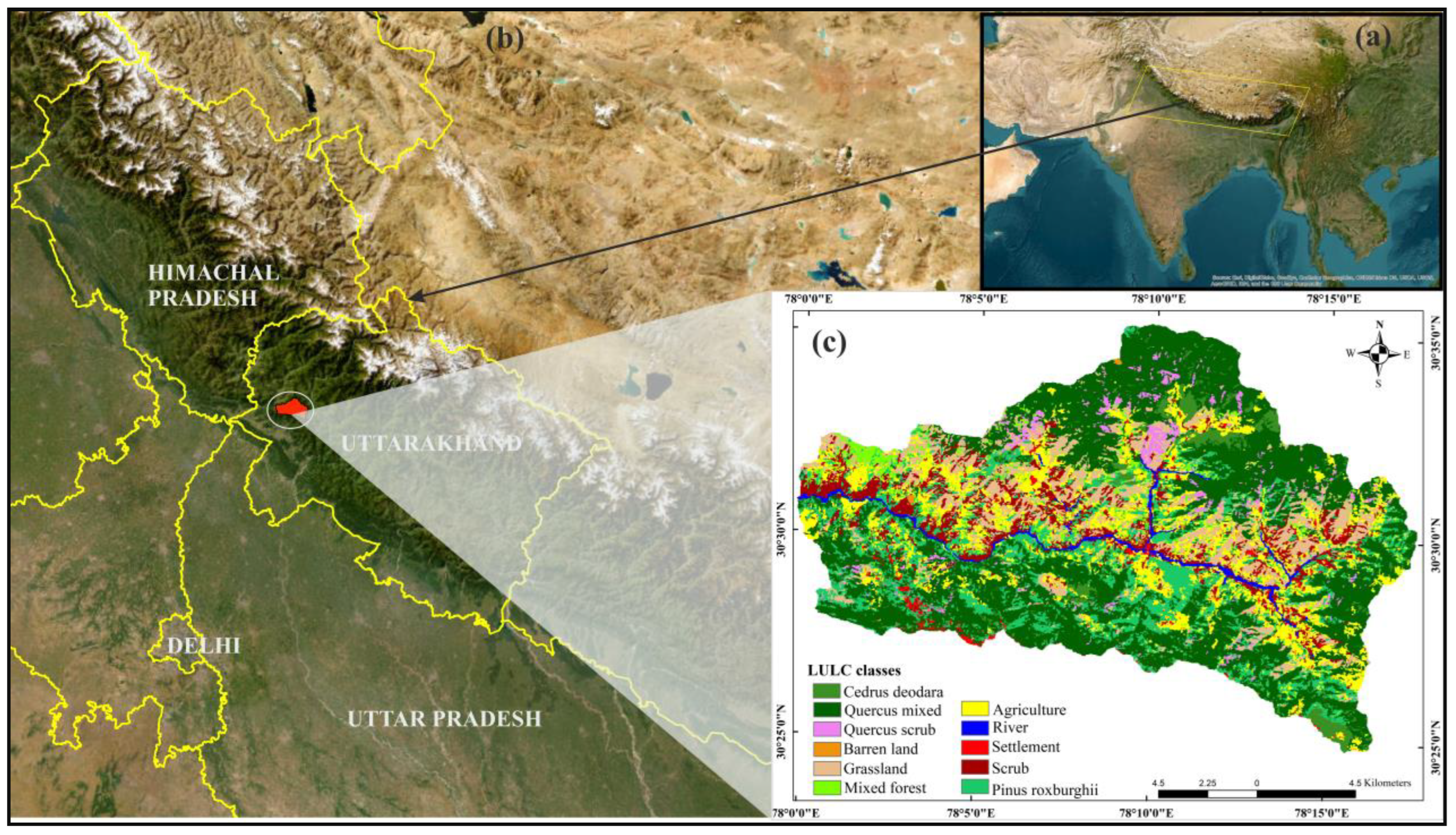
2.1. Study Area

The Aglar watershed, situated in the Tehri-Garhwal district of Uttarakhand, India, covers an approximate area of 307.6 km² (Figure 1). Positioned within the geographic coordinates of 30°27′4″N to 30°38′5″N latitude and 77°56′15″E to 78°18′45″E longitude, the watershed primarily consists of hilly terrain. The area is predominantly used for agricultural purposes, particularly in the flood plains, with elevations ranging from 600 m to 3022 m above sea level. The drainage system of the region is characterized by parallel, sub-parallel, and sub-dendritic streams, which are sustained by numerous perennial streams. Soil variations in the watershed range from reddish-brown to dark brown, exhibiting slight to moderate acidity and a propensity for degradation [27]. Climatically, the watershed transitions from subtropical conditions at lower elevations to more temperate climates at higher elevations, with an annual average rainfall exceeding 2000 mm and temperatures fluctuating between 6 °C and 20 °C. The major forest types as identified by [45] include Oak mixed forests (Quercus leucotrichophora and Quercus floribunda), moist temperate coniferous forests (Cedrus deodara), tropical coniferous forests (Pinus roxburghii), and mixed species forests.

2.2. Methodology

2.2.1. Spatial Mapping of Indicators of HES

In the present study, we estimated six major hydrological flux components to corresponding HES descriptors (detailed in

Table 1. Categorization of hydrological flux components in HES descriptor with proper justifications.

ESs Categories (Definitions)	HES Descriptors	Hydrological Flux Components	Justifications
Provisioning Services (Raw, tangible materials or resources produced by natural ecosystems and directly utilized by humans)	Water yield (WYLD) (+).	Water yield components includes the sum of surface runoff, base flow, ground water contribution, net transmission losses	These are ecosystem goods responsible for providing freshwater for sustaining life both for flora and fauna
Regulating Services (Benefits obtained from the regulation of ecosystem processes)	Total water retention (TWR) (+) An aggregate of soil water retained in soil profile and percolation. Surface Runoff (SURFQ) (−), Base flow (LATQ) (+)	Hydrological fluxes in their individual capacities, including net water retained during the year, the surface runoff leaving the catchment, and base flow that regulates the climate	The regulating needs are environmental flow, soil moisture regime for growth of life
Supporting Services (Services those are necessary for the production of all other ESs)	Sediment yield (SYLD) (−) Crop productivity regulated by (1-AET/PET), i.e., Crop yield response factor (CYF) (+)	Sediment yield and AET and PET components	SYLD surrogate indicators for retaining of the soil due to reduced erosion. Hydrological proxy for net primary productivity (NPP).

‘+’or ‘−’ signs refer to the favorable and non-favorable contribution to the HES figures.

) in Aglar watershed using water balance equation (Equation (1)). These descriptors were as follows: water yield (WYLD), total water retention (TWR), surface runoff (SURFQ), base flow (LATQ), sediment yield (SYLD), and crop yield response factor (CYF). The ArcSWAT version 2012.10_4.21 was used in ArcGIS 10.4.1 software to setup SWAT model developed by [46] to analyze the hydrological flux components in the watershed. The TWR was calculated by assessing soil water in the soil profile and percolation, derived from the water balance equation whereas SYLD was estimated through the Modified Universal Soil Loss Equation (MUSLE) (Equation (2)), formulated by [47] and later modified by [48].

$$S{W}_t=S{W}_0+{{\displaystyle \sum }}_{i=1}^t(R_{day}-Q_{surf}-E{T}_i-W_{seepi}-Q_{gw})$$

(1)

Here, $S{W}_t$ stands for final soil water content (mm), $S{W}_0$ is the initial soil water content (mm), $R_{day}$ is the precipitation (mm), $Q_{surf}$ is the surface runoff (mm), $E{T}_i$ is the evapotranspiration (mm), $W_{seepi}$ is the amount of water entering (mm) to the vadose zone of the soil profile, and $Q_{gw}$ is the amount of return flow (mm) for the specific day i.

SYLD = 11.8 × (Q_surf × q_peak × area_hru)^0.56 × K_USLE × C_USLE × P_USLE × LS_USLE × CFRG

(2)

Here, SYLD = sediment yield (tons), Q_surf = surface runoff (mm/ha), q_peak = peak runoff rate (m³/s), area_hru = area of HRU (ha), K_USLE = USLE soil erodibility factor, C_USLE = USLE cover and management factor, P_USLE = USLE support practice factor, LS_USLE = ULSE topographic factor, and CFRG = Coarse fragment factor.

As Aglar is an ungauged watershed, calibration of hydrological parameters was performed using nested regionalization technique which involved partitioning of sub-watersheds of gauged watersheds (i.e., donor) into batches on the basis of their contribution to the outlet sites that are required to be calibrated [49]. Further, the calibration is performed based on the physical similarities such as soil, land use, topography, and elevation among donor and recipient watersheds. This involves transfer of hydrological parameters from a calibrated donor watershed to an ungauged (recipient) watershed to predict the hydrological response [27,50,51,52,53]. In this study, the Bausan watershed served as the donor, calibrated with observed stream discharge data obtained from Central Water Commission (CWC) New Delhi at two hydrological station sites (Bausan and Naugaon). The Aglar watershed, part of the larger Bausan watershed, was calibrated using stream discharge data collected at the outlet of the Aglar, after calibrating Bausan watershed. The performance of the SWAT model, utilizing observed monthly discharge data from the station, was evaluated through various model statistics. For the calibration period (2005–2011) at the Naugaon station site, the model achieved coefficient of determination (R²) = 0.79, Nash Sutcliff Efficiency (NSE) = 0.61, and standardized root mean square error (RSR) = 0.63. During the validation period (2012–2015), the model statistics were R² = 0.68, NSE = 0.50, and RSR = 0.57. In comparison, the Bausan station site recorded R² = 0.85, NSE = 0.81, and RSR = 0.43 for calibration, with the validation period yielding R² = 0.82, NSE = 0.78, and RSR = 0.35. The percent bias (Pbias) values for the Bausan site were notably satisfactory, at 23.46 and 24.63 for the calibration and validation periods, respectively. However, at the Naugaon station, the Pbias values were higher, at 38.4 and 39.53 for calibration and validation periods, respectively, indicating uncertainties in stream flow measurements. Despite the elevated Pbias values, all other performance metrics were within acceptable ranges at both sites. Additionally, the model performance was assessed at the Aglar outlet, where the calibration period yielded an R² of 0.91, NSE of 0.91, RSR of 0.29, and a Pbias of 2.30. During validation, the figures were R² = 0.68, NSE = 0.50, RSR = 0.37, and Pbias of −1.50. These performance statistics are categorized as “very good”, as per the criteria established by [54]. After successfully parameterizing the SWAT model, a 30-year long-term simulation spanning from 1986 to 2015 was performed in order to capture the long-term variations in the hydrological fluxes of Aglar watershed. Further, well-calibrated and validated hydrological parameters of Aglar were used to map HES descriptors at Hydrological Response Unit (HRU) scale in ArcGIS software. For complete details on the SWAT model parameterization, calibration, validation, uncertainty, and sensitivity analysis of parameters for the Aglar watershed, please refer to [27].

In consideration of factors such as land cover type, rainfall intensity, soil erosivity, and crop management practices, SYLD emerges as an inverse indicator of sediment retention service, as delineated by [55]. SYLD, denoting soil loss per unit area, serves as a proxy for soil retention capacity. Therefore, the SYLD rate corresponding to specific land use categories offers valuable insights into the sediment retention potential of distinct land use types.

In HES context, we hypothesized provisioning services typically consist of raw materials immediately derived from the ecosystem. This includes all water components that leave a landscape following an event and are used beneficially, often representing “fast variables” that are crucial for sustaining life, such as water yield. On the other hand, supporting services involve “slow variables”, which are enhancements of a service resulting from the long-term manifestation of a variable, like soil formation. Here, sediment yield serves as a proxy. Regulating services combine both “slow” and “fast” hydrological variables that help manage environmental conditions. For instance, water retained in the soil serves as a proxy for soil moisture, which is vital for regulating the carbon cycle, surface runoff, and base flow, which are crucial for maintaining environmental flows. The hydrological components, often multi-counted in different service categories, suggest that each inherits characteristics from its service class. This significance is then cumulatively emphasized in their overall contribution. When examining the variety of HES descriptors, it is important to consider both their positive and negative contributions in water balance, as shown in Table 1. Components like base flow, groundwater flow, and runoff are accounted for under multiple service categories. As previously noted, the way these contributions are quantified depends on the weights assigned to each service when calculating the final value of ESs.

2.2.2. Hot and Cold Spots Identification Approaches

Upon successful configuration of the SWAT model, HES descriptors were estimated and mapped at the HRU scale for the entire Aglar watershed. Subsequently, these estimates underwent zonal averaging, with each zone representing a distinct land use parcel within the watershed area. The data were structured in matrix form, with rows representing land use classes and columns representing HES descriptors. Assuming there are n (i = 1, 2,…, n) distinct land use classes, each associated with m (j = 1, 2,…, m) HES descriptors, the variable x_ij denotes the values of HES descriptors for the i^th land use and j^th HES descriptor, resulting in a final matrix of dimensions n × m. Subsequently, these descriptors were normalized on a scale of 0 to 1, where higher values correspond to areas with maximum service supply (x_ij,max), and lower values correspond to areas with minimum service supply (x_ij,min). If the variable exhibits a positive functional relationship with the final HES, normalization can be accomplished using Equation (3).

$$X_{ij,norm}={\displaystyle \frac{\left(x_{ij}-x_{ij,min}\right)}{(x_{ij,max}-x_{ij,min})}}$$

(3)

For a negative functional relationship, Equation (3) is just replaced by $1-X_{ij,norm}$, where $X_{ij,norm}$ is the index for the i^th HES descriptors for j^th land use class.

Altogether, final HES descriptor for each of the land use segment i (HES_i) can be defined using Equation (4):

$$HE{S}_i={\displaystyle \sum }_{j=1}^m\left[w_j{x_{ij}}_{norm}\right]$$

(4)

where $w_j$ = weightage of the HES descriptors.

2.2.3. Assigning Weights to HESs

The uncertainty associated with assigning weights to different ESs stems from several factors. Firstly, there may be inherent subjectivity in the weighting process, as different stakeholders or experts may prioritize services differently based on their perspectives, values, and goals. Additionally, the complexity of ecosystem dynamics and interactions may introduce uncertainty regarding the true significance or contribution of each service to overall ecosystem health and functioning. Furthermore, variations in methodologies used to estimate weights can also contribute to uncertainty. Different weighting methods may yield divergent results based on their underlying assumptions, data inputs, and algorithms. Uncertainty may also arise from limitations in data availability, quality, or representativeness, particularly for less studied or poorly understood Ecosystem Services. To tackle these challenges, different weight assignment methods were employed to assign weights such as equal weight, unequal weight, Analytical Hierarchy Process (AHP), and Principal Component Analysis (PCA), with each method explained in detail henceforth. The analysis was performed in two categories: Category 1 involved assigning weights to each HES individually using the four methods, while Category 2 involved grouping the HES into three major ESs classes—provisioning, regulating, and supporting services—as defined by [3] and then assigning weights for hot and cold spot delineation using the same four methods. This approach of using multiple methods to assign weights helped identify the inherent uncertainties in describing HES for each land use category.

• Approach 1: Equal weight (EW method)

In this method, all the hydrological flux components were considered equally important and thus a uniform common weight was assigned to each of them using simple average of all the normalized scores (Equation (5)).

$$\mathrm{Wi}={\displaystyle \frac{{{\displaystyle \sum }}_j{X}_{ij}+{{\displaystyle \sum }}_j{y}_{ij}}{K}}$$

(5)

where $X_{ij}$ is the value of indicator j corresponding to region i in a matrix and $y_{ij}$ is equal to 1 − $X_{ij}$ and K is the number of HES descriptors used.

• Approach 2: Unequal Weights (Iyengar and Sudarshan’s method)

For unequal distribution of weights, Iyengar and Sudarshan’s (I and S) approach [56] was used, which assumes that weight of the respective indicators vary inversely with respect to the variance (Equations (6)–(8)). Assignment of weight using this method ensures that large variations in any one of the indicator will not dominate the contribution of the others. This method serves as a more simple approach to classify indicators in comparison to complicated methods like PCA, which are based on restrictive assumptions.

$$Y_i={\displaystyle \sum }_{j=1}^k{w}_j\times x_{ij}$$

(6)

$$w_j={\displaystyle \frac{c}{\sqrt{\mathrm{Var}i\left(x_{ij}\right)}}}$$

(7)

$$c={\left[{\displaystyle \frac{{{\displaystyle \sum }}_{j=1}^{j=k}1}{\sqrt{\mathrm{Var}i\left(x_{ij}\right)}}}\right]}^{-1}$$

(8)

where $w$ is the weights (0 < $w$ < 1, and ${\displaystyle \sum }_{j=1}^k{w}_j=1).$

• Approach 3: Analytical Hierarchy Process (AHP method)

Pair wise comparison matrix based on AHP is a ratio matrix technique developed by [57], where weights were calculated on the scale of 0 to 9 depending upon the importance one over another. Further, the matrix consistency was then judged on the basis of indices given from Equations (9)–(11):

$$\mathrm{Consistency} \mathrm{index}={\displaystyle \frac{{\mathsf{\lambda }}_{\max }-\left(n\right)}{n-1}}$$

(9)

$$\mathrm{Ratio} \mathrm{index}={\displaystyle \frac{\overrightarrow{{\mathsf{\lambda }}_{\max }}-\left(n\right)}{n-1}}$$

(10)

$$\mathrm{Consistency} \mathrm{ratio}={\displaystyle \frac{{\mathsf{\lambda }}_{\max -}\left(n\right)}{\overrightarrow{{\mathsf{\lambda }}_{\max }}-\left(n\right)}}$$

(11)

The matrix with index value < 0.01 was considered consistent.

• Approach 4: Principal Component Analysis (PCA method)

PCA is defined as a multivariate statistical method with the goal to extract important information from the dataset, which is represented as a set of new orthogonal variables through orthogonal transformations called principal components (PC) or eigenvectors. PCA keeps the maximum variance in the dataset intact after performing orthogonal transformations. The orthogonal transformations help in segregating the set of the most correlated parameters into a set of linearly noncorrelated parameters. It is thus useful in highlighting the common pattern and complexity of the data by reducing the redundancies, aiding its effortless interpretation. This study used “FactoMineR”, “Factoextra” packages in R environment to determine the contribution of individual flux component under each service category. Following PCA, the highly weighted variable/indicator in a PC was determined by weighting of the parameters calculating the Euclidean distances of the variables in a bi-plot of PC1 and PC2 dimensions.

Specific weights were assigned to each HES descriptor in two categories. The first category (i.e., method-1) allocated weights under the assumption that the variability of each six descriptor individually sums up to 1. The second category (i.e., method-2) grouped the HES descriptors into three broad ESs categories (as mentioned in Table 1), with each category considered equally important and assigned a uniform weight of 0.33. Within each ESs category, HES descriptors received weights on a pro-rata basis according to previously defined approaches. Weights obtained from each approach were then applied to the normalized maps of HES descriptors in both the methods. Further, average and median values of these approaches were computed; however, median values were preferred over average and a single hot spot and cold spot map was produced under each method. These maps were then classified into five classes—very high, high, moderate, low and very low—representing the areas of hot (i.e., very high) and cold spots (i.e., very low). As the result of using multiple weightage approaches in assigning weights to the HES descriptors, uncertainties at pixel-level arise, which were assessed by overlaying the consistent pixels of cold and hot spots present in each approach through mode values. The pixel values of each weightage map derived from different approaches in method 1 and 2 were classified into five classes and were overlaid to extract consistent pixel-values (or modal class) to determine pixel-level uncertainties in the HES hot and cold spot maps.

2.2.4. Trade-Off and Synergy Analysis among HES

To investigate the trade-offs and synergies among HES, we applied the Pearson correlation coefficient to analyze linear relationships between different HES. This involved generating 500 random points across the geographic distribution of HES to ensure a broad and representative sample of the HES spatial variations. At each of these points, we extracted the corresponding values for six HES, which is critical for collecting precise data necessary for assessing the interactions between services at specific locations. Positive coefficients indicate synergistic relationships, where enhancements in one service positively influence another, while negative coefficients reveal trade-offs, indicating a detrimental impact on one service due to the increased use of another. This approach provides a detailed examination of how different HES interact across space, aiding effective ecosystem management and decision-making.

3. Results

The spatial distribution of key hydrological components considered in this study for the analysis of hot and cold spot showed variation across the Aglar watershed. The precise partitioning of hydrological flux components is essential for understanding their impact on water availability and flow regulation in terrestrial ecosystems. This helps quantify contribution of each component in provision of the ESs [27]. The SWAT model was utilized to analyze the annual water balance of the Aglar watershed, which received an average precipitation of 1392 mm distributed across various hydrological fluxes, with 36% contributing to stream flow, consisting of 72% direct runoff and 28% base flow. There was a variation in the spatial distribution of fast variables such as WYLD, ranging from 241.21 to 728.75 mm, LATQ from 4.35 to 121.49 mm, and TWR from 236.18 to 456.76 mm across different land use categories of the Aglar watershed (Figure S1). Agricultural land was the largest contributor to WYLD, followed by Oak and Deodar forests, while Pine forests had lower contributions. Oak mixed and Deodar mixed forests exhibited better LATQ and TWR compared to agriculture and grasslands. The AET in Aglar ranged from 541.54 mm to 1092.2 mm. Broad leaf forests like Oak had the highest AET, while other land use had lower AET requirements. Slow variables such as average SURFQ varied from 148.99 mm to 666.02 mm, and sediment yield ranged from 0.03 to 25.79 t/ha across different topographic and land use segments. Regions with significant SURFQ and SYLD included agriculture, pine forests, and scrublands, whereas Oak mixed and Deodar forests had lower SURFQ and SYLD compared to other land uses. These maps of HES descriptors were normalized based on the approach outlined in the Methodology section, and, subsequently, weights were assigned for identification of hot and cold spot areas in the Aglar watershed, which are detailed hereafter. For more detailed information on spatial variation in HES values in the Aglar watershed, please refer to [27].

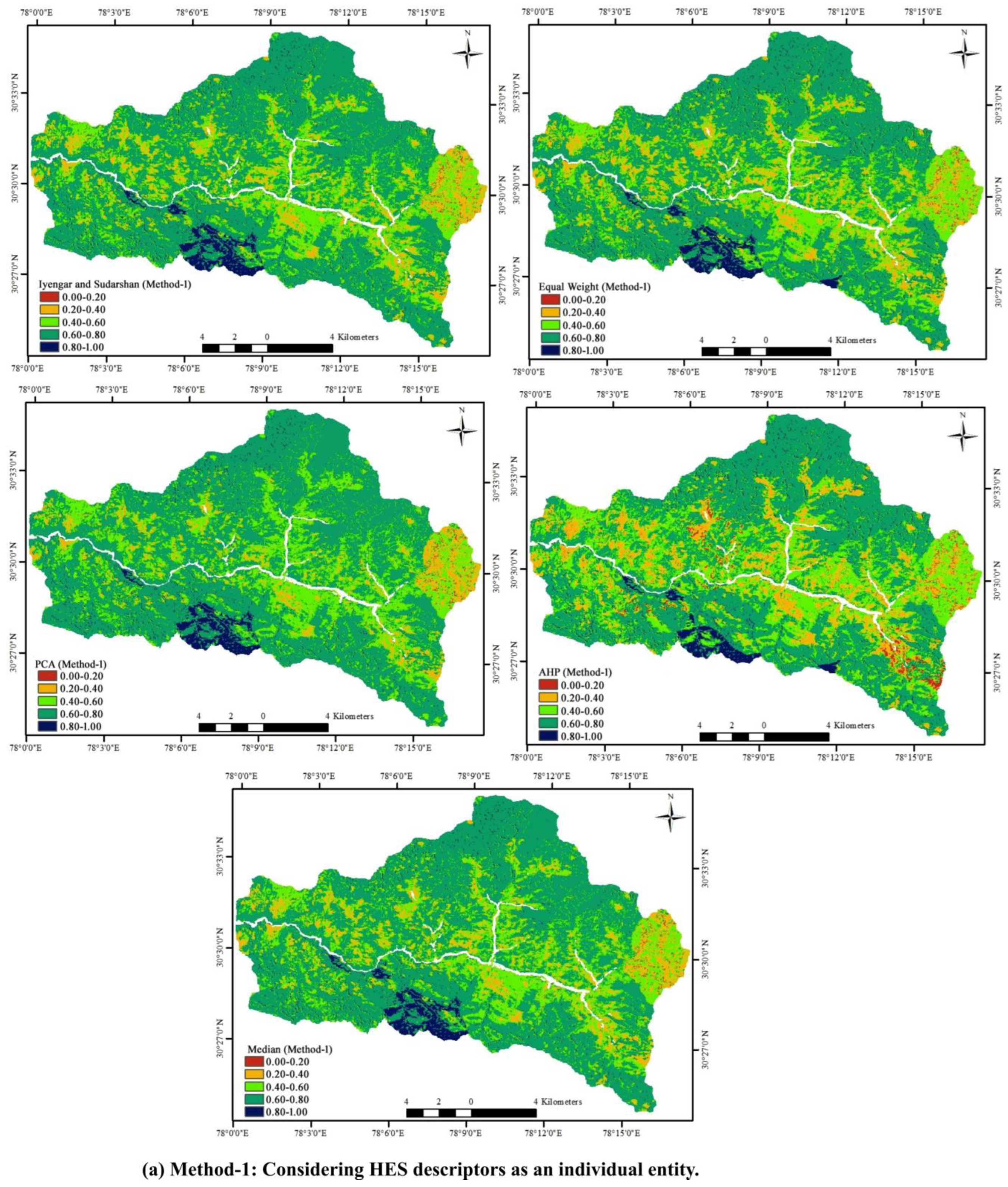
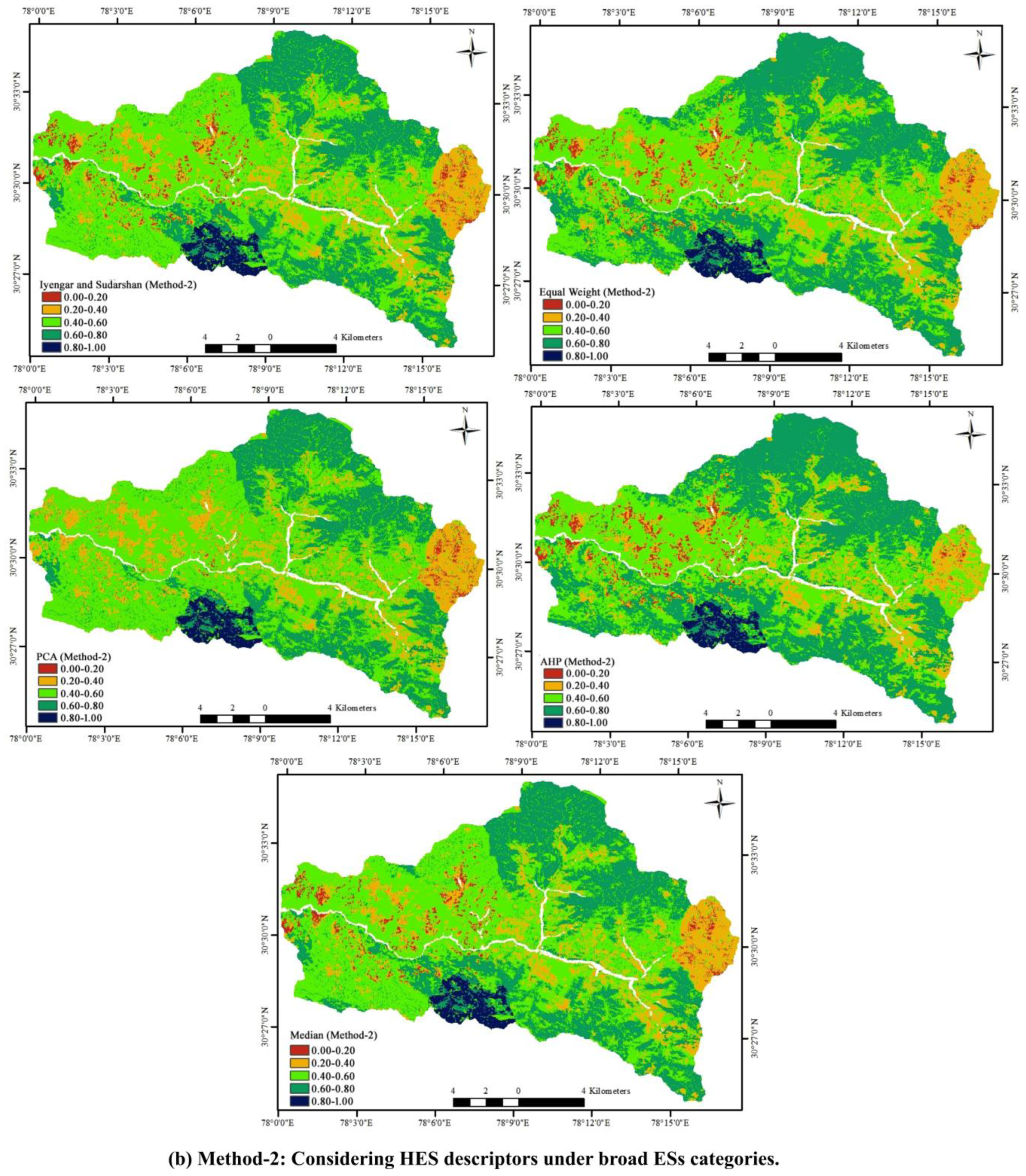
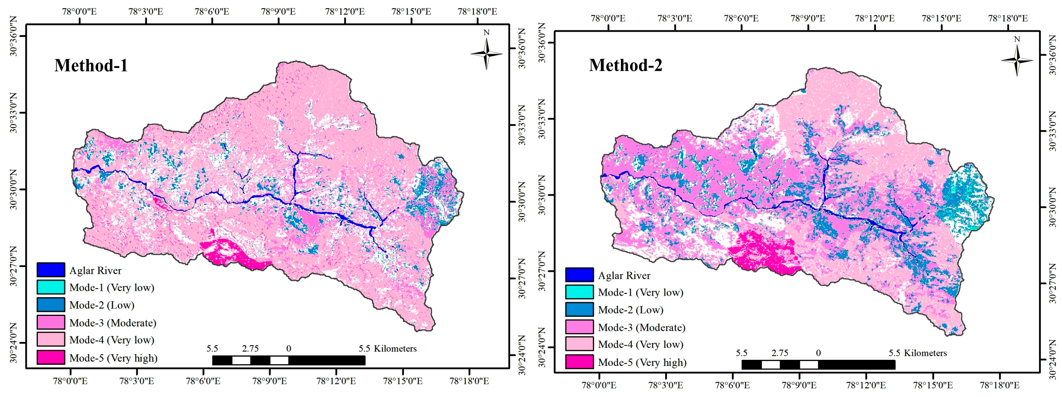
3.1. Identification and Spatial Mapping of Hot and Cold Spots Regions of HES

Table 2. Weights of individual HES descriptors with respect to their variability inheriting the weights as an individual entity.

		HES Descriptors
Weightage Methods	WYLD	TWR	SURFQ	LATQ	SYLD	CYF = 1 − AET/PET	Sum
I and S	0.176	0.144	0.177	0.163	0.161	0.178	1.0
EW	0.167	0.167	0.167	0.167	0.167	0.167	1.0
PCA	0.180	0.145	0.188	0.154	0.147	0.186	1.0
AHP	0.147	0.187	0.146	0.189	0.178	0.152	1.0
Median	0.1715	0.156	0.172	0.1649	0.1640	0.1722	1.0

illustrates the variability in weights assigned to individual HES descriptors using different weighting approaches. The I and S approach assigned the highest weight to CYF (0.178) and the lowest to TWR (0.144). The EW approach treated all HES descriptors as equally important, assigning a uniform weight of 0.167 to each. The PCA approach gave the highest weight to SURFQ (0.188) and the lowest to TWR (0.146). In the AHP approach, LATQ received the highest weight (0.189), while SURFQ received the lowest (0.146). Notably, CYF consistently had the highest median value across all approaches. This comparison helps understand the relative importance of each HES descriptor as evaluated by different standard methods.

Table 3. Weights of individual HES descriptors assuming their service sub-class inherits the weights as an individual entity.

	Provisioning Service (0.33)	Regulating Services (0.33)			Supporting Services (0.33)
	HES Descriptors
Weightage Methods	WYLD	TWR	SURFQ	LATQ	SYLD	CYF = 1 − AET/PET	Sum
I and S	0.330	0.098	0.120	0.111	0.157	0.173	1.0
EW	0.330	0.110	0.110	0.110	0.165	0.165	1.0
PCA	0.330	0.098	0.127	0.104	0.146	0.184	1.0
AHP	0.330	0.118	0.092	0.120	0.178	0.152	1.0
Median	0.330	0.104	0.115	0.111	0.161	0.169	1.0

demonstrates the variability in estimated weights for HES descriptors, considering each service sub-class as an individual entity and employing diverse approaches. All three service categories were deemed significant. Within these categories, WYLD, the sole entity under the provisioning services category, consistently held a weight of 0.33 across all approaches. In the regulating services category, the weights for TWR, SURFQ, and LATQ were estimated. SURFQ obtained the highest weight (0.127) from the PCA approach but the lowest from the AHP approach (0.092). Similarly, weights obtained for TWR were relatively low from both the I and S and AHP approach, at 0.098 and 0.118, respectively. For supporting services, sediment retention (SR) with a proxy of SYLD and CYF were scrutinized; CYF received a high weight from the PCA approach (0.184) but a lower weight (0.152) from the AHP approach. In the EW approach, all HES descriptors within each category were assigned equal weights. Additionally, CYF consistently exhibited the highest median value across all approaches in category-wise hot spot and cold spot analysis.

Unlike other methods that adhere to their standard computational approaches, the weights assigned by PCA remained consistent with the methodologies in previous approaches. When examining the six descriptors, PCA revealed that SURFQ made the most significant contribution, followed by WYLD and CYF, as depicted in Figure 2a. This visualization illustrates the relative distances of the variables from the origin, shifted along PC1 (61.50%) and PC2 (14.29%), which together accounted for over 75% of the variance. Furthermore, within the category of regulating services, TWR exhibited the highest variance contribution (72.63%), followed by LATQ and SURFQ, as shown in Figure 2b. In the case of supporting services consisting of two variables only, the percent contribution of each variable in each dimension was equal, as shown in Figure 2c.

Figure 3a,b depict the spatial distribution of hot and cold spot areas in the Aglar watershed using four different approaches, along with their median values. The value ranges from 0.0 to 1.0, with lower values indicating cold spots and higher values indicating hot spots. In method-1, the spatial pattern of hot and cold spots was found to be relatively consistent among the approaches, particularly in areas showing high to very high hot spot values. The hot spots with very high values were predominantly located in the southern region of the watershed and along the Aglar river, while high value hot spots covered the most areas of the watershed. The distribution of these areas was most distinctly observed using the AHP and EW approach, which clearly delineated the critical areas in comparison to other approaches in method-1. Other approaches did not adequately highlight very low values corresponding to cold spots. Under method-2, the distribution of hot and cold spots varied. Similar to method-1, the very high value hot spots were concentrated in the southern region of the watershed. However, the distribution of cold spots differed significantly depending on the approach in method-2. The PCA, EW, and SI approaches revealed that regions with very low to low values, representing cold spots, were more concentrated on the eastern side of the watershed. Notably, the PCA approach identified a dominant pattern of hot and cold spots on the eastern side of the watershed. Additionally, the PCA, S and I, and AHP approaches indicated that areas with very high to high service values were primarily located in the northeast, east, and southeast regions of the watershed. Under method-1, the areas classified as very low to low in terms of median values cover approximately 30.73 km², representing about 10.3% area of the watershed. Conversely, the majority of the watershed, or about 193.34 km² (approximately 64.83%), falls into the very high to high median class. Approximately, 0.3% of the watershed area was classified as cold spots, and 3.18% as hot spots, exclusively under the very low and very high median classes, respectively, using method 1. In contrast, with method-2, the areas classified as very low to low median values encompass about 51.19 km², which contributes around 17.17% to the total area of the watershed. However, the regions falling under the very high to high median class account for about 98.63 km², or approximately 33.07% of the watershed. Using method 2, approximately 2.42% of the watershed area was classified as cold spots and 2.36% as hot spots, based on the very low and very high median classes, respectively. The Hot and cold spot areas under distinct median classes obtained from method 1 and 2 are detailed in

Table 4. Hot and cold spot areas under distinct median classes obtained from method 1 and 2.

			Method-1		Method-2
Sl. No.	Median Class	Median Categories	Area (km2)	% Area Contribution	Area (km2)	% Area Contribution
1	0.0–0.2	Very low	0.79	0.268	7.23	2.42
2	0.2–0.4	Low	29.94	10.04	43.96	14.74
3	0.4–0.6	Moderate	74.14	24.86	148.39	49.76
4	0.6–0.8	High	183.86	61.65	91.58	30.71
5	0.8–1.0	Very high	9.48	3.18	7.05	2.36

.

3.2. Pixel-Level Uncertainty in Hot and Cold Spot Maps

Table 5. Area under different modal classes obtained for method-1 and method-2.

		Method-1	Method-2
Mode Class	Mode Categories	Area (km2)	Area (km2)
1	Very low	0.57	2.30
2	Low	13.35	34.92
3	Moderate	45.23	113.79
4	High	154.62	80.46
5	Very high	6.86	6.97

indicates the distribution of areas across different modal classes obtained from both the methods. The pixels consistently contributing to very high category areas (i.e., hot spots) are nearly identical in both the methods; however, pixels consistently contributing very low category areas (i.e., cold spots) varied in both the methods. Method 1 resulted in significant area classified under high, whereas method 2 has larger areas in the low and moderate categories. This distribution aids in comprehending how each method classifies the watershed area into varying significance levels of ESs. Furthermore, it verifies the authenticity of the hot and cold spot regions of HES in the watershed, regardless of methodological uncertainties. The maps shown in Figure 4 highlight the consistent pixels obtained as hot and cold spots in all approaches from both the methods, whereas the blank areas were the inconsistent pixels with different values in each approach.

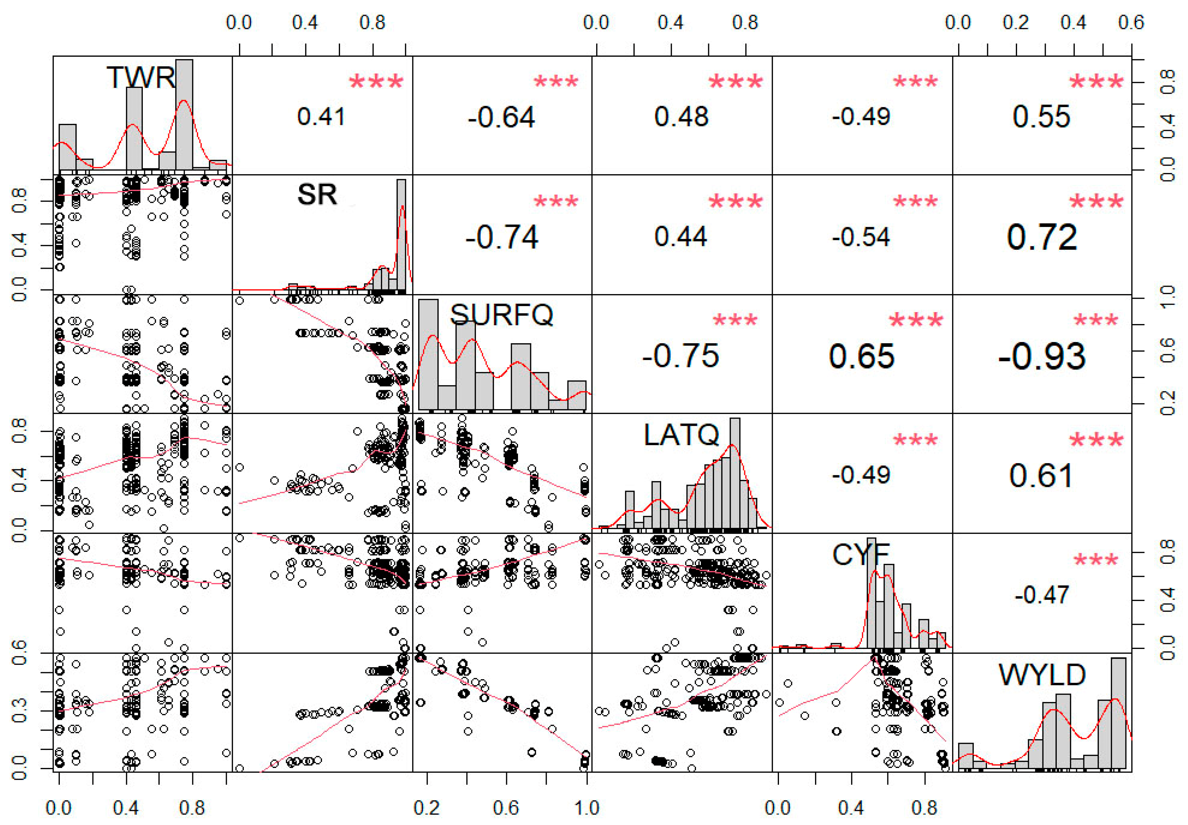
3.3. Trade-Offs and Synergies Analysis

To analyze the complex interdependencies among ESs, the relationships and interactions among six HES were examined using Pearson correlation, as depicted in Figure 5. This analysis revealed notable synergies and trade-offs between different HES descriptors. A synergistic relationship, indicated by correlation coefficients greater than 0.6, was found between LATQ and WYLD (0.61) and between sediment retention (SR) and WYLD (0.72). SURFQ displayed a synergistic relationship with CYF (0.65), suggesting a beneficial interaction between these two descriptors. These positive correlations suggest that improvements in one service are associated with enhancements in the other, highlighting mutual benefits. Conversely, significant trade-off relationships among HES descriptors were also identified, where increases in one service are linked to decreases in another characterized by negative correlation coefficients. The most pronounced trade-off was observed between SURFQ and WYLD (−0.93). Other notable trade-offs included SURFQ and LATQ (−0.75), SURFQ and SYLD (−0.74), and SURFQ and TWR (−0.64).

4. Discussion

The study offers a comprehensive methodology for identifying hot and cold spots of HES based on their descriptors in the Aglar watershed of the IHR. Utilizing a multiple weightage approach to assign weights to the HES descriptors, the delineation of hot and cold spots highlights the critical importance of selecting appropriate methods for accurate assessments. Pixel-level uncertainties in the hot and cold spot maps were also identified, providing a nuanced understanding of their spatial variability. Furthermore, the evaluation of trade-offs and synergies enhances our comprehension of the complex dynamics within the watershed, thereby promoting informed decision-making for sustainable watershed management.

The spatial variations observed in the critical areas of hot and cold spots of HES are influenced by several factors such as land use, soil properties, topography, and climate. Each of these factors individually and collectively plays a significant role in the hydrological functions of the watershed, and their effects are more pronounced in rugged terrains like Aglar. Different land parcels, such as forests, agriculture, settlements, and barren land, contribute differently to the HES descriptors, thereby affecting the spatial patterns of hot and cold spots. In this case, the very high to high hot spot zones in the watershed mainly comprised forested land in continuous patches. Specifically, evergreen broadleaf forests, like Oak mixed forests, and evergreen needleleaf forests, like Deodar forests, exhibit high service supplies, which dominate the watershed and form part of the hotspot regions. The percent contribution of land use classes to HES descriptors is shown in

Table 6. Median weights and % contribution of land use classes to all HES descriptors.

Sl No.	Land Use Classes	Median Weights	% Contribution of Land Use
1	Agriculture	0.515	5.8
2	Cedrus deodara forest	1.467	16.6
3	Mixed forest	1.299	14.7
4	Grasslands	1.292	14.6
5	Quercus forest	1.657	18.8
6	Pinus roxburghii forest	1.193	13.5
7	Scrubs	1.415	16.0

. Cooler climates, favorable slopes, optimal sunlight exposure, soil moisture, and humidity conditions, along with the structural characteristics of Oak forests—such as layered canopies and deep root systems—significantly enhance the soil’s water retention capabilities, unlike other land use categories like agriculture and scrubs [27,58,59]. Similar findings were reported by [60,61,62] through spatially explicit analyses of ESs under different scenarios of land use change and trade-off analyses among ESs.

Approaches to manage ESs can vary based on the specific objectives and context of the study. An individual services approach enables a detailed understanding of each ES, allowing for tailored management strategies and more effective conservation and utilization practices. Singular approach also facilitates the identification of trade-offs between services, which is essential for making well-informed decisions. However, managing each service individually can be challenging and require significant resources. On the other hand, considering broad ESs categories like provisioning, regulating, and supporting offers a generalized technique. This approach provides a holistic view of ecosystem functioning, highlighting broader patterns and trends, and is more resource-efficient. It reduces the complexity of the analysis, making it more helpful for policy-making and management purposes [63]. Therefore, a potentially better approach might involve a hybrid strategy, where analyses are performed by grouping ESs into broad categories while also conducting more detailed analyses of individual services that are particularly important or problematic. Such integrated management strategies ensure a balanced and comprehensive understanding, leading to more effective management and conservation efforts.

Unlike many studies that have utilized threshold techniques to map hot and cold spots of ESs using the highest quantile, Gi* statistics, or other spatial clustering methods, this study employed a multiple weightage approach for hot and cold spot delineation. These methods tend to produce less dispersed critical areas of ESs and are more beneficial for areas with good spatial connectivity [8,24]. The outcomes derived from the intensity approach, which assesses various ESs in relation to each other, exhibited greater variability throughout the study area, resulting in a significantly reduced total selected area. This methodology takes into account the diversity of ESs and as a result identifies areas where these services intersect [8]. Among the weightage approaches used in this study, SURFQ received the highest weight from the unequal and PCA approaches, whereas AHP resulted in the highest weight for LATQ. AHP is an expert knowledge-based approach that incorporates the perspectives of various experts into the mapping process. The difference in the weightage pattern observed in AHP was attributed to its high levels of subjectivity among the experts [64].

Additionally, the preference for using the median over the mean arises in scenarios dealing with data prone to skewness or outliers. Unlike the mean, the median is less influenced by extreme values, making it a robust measure of central tendency in such cases [65,66]. This robustness is particularly advantageous when analyzing datasets with skewed distributions or outliers, where the mean may be distorted by these extreme values. The median is also well suited for ordinal or categorical data, where numerical calculations might lack interpretability. In situations where the data does not adhere to a normal distribution, the median often proves to be a more reliable indicator of the central tendency compared to the mean. However, the choice between median and mean ultimately depends on the nature of the dataset and the specific objectives of the analysis, with each measure offering unique insights depending on the context.

When conducting regional-level analysis of ESs, uncertainties are inevitable [63]. In this study, we identified variations in the quantification of HES descriptors and the use of multiple weighting approaches as two primary sources of uncertainty. Each weighting method introduces errors that propagate to the outcomes. In method 1, all HES descriptors were given equal status, with variations in assigned weights arising from intrinsic differences in the approaches. The hydrological components of the watershed, influenced by land use, significantly impacted the uncertainty map. Consequently, a majority of pixels were classified under the high modal class, mainly in forested areas in the Aglar watershed, which is the dominant service provider land use class. Conversely, HES descriptors categorized by method 2 were grouped under broader ESs categories, which proved to be a more effective approach. This aligns with the recommendations of [63], who suggested that examining overall trends between ESs may be more informative than focusing on individual ESs.

ESs are interconnected in both space and time, creating intricate relationships that can result in either trade-offs or synergies [67]. Synergies occur when one ES enhances another, while trade-offs happen when the provision of one ES diminishes the benefits of another [68]. Significant positive relationship showing synergies among the HES indicators was observed in this study, such as SURFQ and CYF, WYLD and LATQ, and sediment retention and WYLD. Aglar is a mountainous watershed that is predominantly covered by a forest ecosystem. The synergy between CYF (=1 − AET/PET) and SURFQ is influenced by rapid soil saturation, interception by dense canopies, and steep terrain. During periods of heavy rainfall, a higher CYF signifies excess water not utilized for evapotranspiration, leading to increased SURFQ [69]. This phenomenon is more pronounced in mountainous areas due to their steep slope and rugged topography, causing limited soil storage capacity. The synergy between WYLD and LATQ was attributed to the forest ecosystem, which improves infiltration and encourages groundwater recharge. Similarly, the connection between WYLD and sediment retention is driven by the forest soils’ ability to retain water and release it gradually as the stream flows. This is vital for maintaining a consistent water supply, supporting base flow, and ensuring ecosystem health. The root systems of forests enhance soil quality and organic content preventing soil loss, improving infiltration, percolation, and retention, consequently sustaining WYLD and ecological equilibrium.

Significant trade-offs of SURFQ with TWR, LATQ, SR, and WYLD were observed. The trade-off between SURFQ and WYLD was more pronounced. The balance between SURFQ and water percolation, LATQ, and WYLD in the Aglar watershed is influenced by factors such as the forest, steep topography, limited soil storage capacity, and rapid soil saturation during heavy rainfall [27]. The steep slopes in the watershed promote quick SURFQ over percolation. Compared to other land use, forest ecosystem helps with soil structure, sediment retention, and moisture retention. Forests with denser canopy and a thicker litter–humus layer have a greater capacity to intercept rainfall and increase infiltration, thereby greatly reducing SURFQ [70,71]. Although vegetation intercepts rainfall and promotes infiltration, excess rainwater results in overland runoff when the rainfall intensity is higher, the soil permeability decreasing the available water for percolation, groundwater recharge, and sustained LATQ. Recognizing these synergies and trade-offs is crucial for sustainable water resource management, ecosystem preservation, and informed policy development to optimize multiple services concurrently.

5. Conclusions

The study identifies hot and cold spot areas of HES along with the pixel-level uncertainties in them. The study found that median values were more effective than the mean for mapping critical hot and cold spots, as medians were less influenced by outliers. Using median values, approximately 0.26% and 3.18% of the watershed area were classified as cold and hot spots, respectively, using method 1. In contrast, 2.42% and 2.36% of the watershed areas were classified as cold and hot spots, respectively, using method 2. Pixel-level uncertainties revealed that 0.57 km² and 6.86 km² of the watershed are consistently classified as cold and hot spots, respectively, across all approaches in method 1. Likewise, method 2 identified 2.30 km² and 6.97 km² as consistent hot and cold spots. The continuous natural forest cover in the Aglar watershed mainly appeared in hot spots, covering 60% of the area, compared to agricultural or other land uses which resulted in small patches of cold spot regions. The modal analysis in this study highlights the level of uncertainty in classifying hot or cold spots, which are grouped into five equal interval classes ranging from 0 to 1. For method 1 (where individual ES entities are weighted according to specific weight assignment techniques) and method 2 (where the three service classes are equally weighted at 0.33, with the corresponding HES descriptors inheriting weights on a pro-rata basis summing up to 0.33), higher modal values indicate lower uncertainty. For example, a mode of 5 suggests that all five values for the corresponding pixel, based on different weight assignment methods, fall into the same group. Method 1 produces larger areas of the watershed with higher modal values (154.62 km²), indicating it is a more effective approach for classifying hot and cold spots, giving it an advantage over method 2. In addition, it is imperative to state that studying services individually provides detailed insights into their dynamics and interactions, aiding targeted management, whereas grouping services into categories offers a simplified, comprehensive view that aligns with policy and broad conservation strategies. For detailed understanding and targeted actions, individual analysis is ideal, while categorical analysis is better for policy and overall ecosystem insights. Combining both approaches starting with a broad assessment and then focusing on key services can be highly effective. This study also highlights evident synergies and trade-offs among the HES descriptors and emphasizes that the spatial arrangement of hot spot sites may differ based on the identification method. This research underscores the importance of interventions to safeguard forest ecosystems, which contribute significantly to HES, particularly in active terrains like the IHR. It also emphasizes that environmental conditions and human activities significantly influence the flow of ESs. Enhanced clarity on various methodologies, including their advantages and limitations, is crucial for decision-makers to make informed land use decisions, especially in areas requiring immediate attention. Additionally, assigning monetary values to HES benefits can aid in comparing them with other services provided by the landscape under changing environmental conditions and land use–land cover alterations.

References

1. Falkenmark, M. Good Ecosystem Governance: Balancing Ecosystems and Social Needs. In Governance as a Trialogue: Government-Society-Science in Transition; Springer: Berlin/Heidelberg, Germany, 2007; pp. 59–76. [Google Scholar]
2. Mallick, M.; Singh, P.K.; Pandey, R. Harvesting resilience: Tribal home-gardens as socio-ecological solutions for climate change adaptation and sustainable development in a protected area. J. Clean. Prod. 2024, 445, 141174. [Google Scholar] [CrossRef]
3. Millennium Ecosystem Assessment. Ecosystems and Human Well-Being; Island Press: Washington, DC, USA, 2005; Volume 5. [Google Scholar]
4. Francesconi, W.; Srinivasan, R.; Pérez-Miñana, E.; Willcock, S.P.; Quintero, M. Using the Soil and Water Assessment Tool (SWAT) to model ecosystem services: A systematic review. J. Hydrol. 2016, 535, 625–636. [Google Scholar] [CrossRef]
5. Huang, F.; Zuo, L.; Gao, J.; Jiang, Y.; Du, F.; Zhang, Y. Exploring the driving factors of trade-offs and synergies among ecological functional zones based on ecosystem service bundles. Ecol. Indic. 2023, 146, 109827. [Google Scholar] [CrossRef]
6. Cimon-Morin, J.; Darveau, M.; Poulin, M. Fostering synergies between ecosystem services and biodiversity in conservation planning: A review. Biol. Conserv. 2013, 166, 144–154. [Google Scholar] [CrossRef]
7. Gos, P.; Lavorel, S. Stakeholders’ expectations on ecosystem services affect the assessment of ecosystem services hotspots and their congruence with biodiversity. Int. J. Biodivers. Sci. Ecosyst. Serv. Manag. 2012, 8, 93–106. [Google Scholar] [CrossRef]
8. Schröter, M.; Remme, R.P. Spatial prioritisation for conserving ecosystem services: Comparing hotspots with heuristic optimisation. Landsc. Ecol. 2016, 31, 431–450. [Google Scholar] [CrossRef]
9. Schwartz, C.; Klebl, F.; Ungaro, F.; Bellingrath-Kimura, S.-D.; Piorr, A. Comparing participatory mapping and a spatial biophysical assessment of ecosystem service cold spots in agricultural landscapes. Ecol. Indic. 2022, 145, 109700. [Google Scholar] [CrossRef]
10. Brown, G.; Fagerholm, N. Empirical PPGIS/PGIS mapping of ecosystem services: A review and evaluation. Ecosyst. Serv. 2015, 13, 119–133. [Google Scholar] [CrossRef]
11. Huang, Z.; Qian, L.; Cao, W. Developing a novel approach integrating ecosystem services and biodiversity for identifying priority ecological reserves. Resour. Conserv. Recycl. 2022, 179, 106128. [Google Scholar] [CrossRef]
12. Qiu, J.; Turner, M.G. Spatial interactions among ecosystem services in an urbanizing agricultural watershed. Proc. Natl. Acad. Sci. USA 2013, 110, 12149–12154. [Google Scholar] [CrossRef]
13. Bagstad, K.J.; Semmens, D.J.; Ancona, Z.H.; Sherrouse, B.C. Evaluating alternative methods for biophysical and cultural ecosystem services hotspot mapping in natural resource planning. Landsc. Ecol. 2017, 32, 77–97. [Google Scholar] [CrossRef]
14. Lourdes, K.T.; Hamel, P.; Gibbins, C.N.; Sanusi, R.; Azhar, B.; Lechner, A.M. Planning for green infrastructure using multiple urban ecosystem service models and multicriteria analysis. Landsc. Urban Plan. 2022, 226, 104500. [Google Scholar] [CrossRef]
15. Raymond, C.; Curtis, A. Mapping Community Values for Regional Sustainability in the Lower Hunter Region; University of Tasmania: Hobart, TAS, Australia, 2013. [Google Scholar]
16. Van Riper, C.J.; Kyle, G.T.; Sutton, S.G.; Barnes, M.; Sherrouse, B.C. Mapping outdoor recreationists’ perceived social values for ecosystem services at Hinchinbrook Island National Park, Australia. Appl. Geogr. 2012, 35, 164–173. [Google Scholar] [CrossRef]
17. Queiroz, C.; Meacham, M.; Richter, K.; Norström, A.V.; Andersson, E.; Norberg, J.; Peterson, G. Mapping bundles of ecosystem services reveals distinct types of multifunctionality within a Swedish landscape. Ambio 2015, 44, 89–101. [Google Scholar] [CrossRef]
18. Plieninger, T.; Dijks, S.; Oteros-Rozas, E.; Bieling, C. Assessing, mapping, and quantifying cultural ecosystem services at community level. Land Use Policy 2013, 33, 118–129. [Google Scholar] [CrossRef]
19. Onaindia, M.; de Manuel, B.F.; Madariaga, I.; Rodríguez-Loinaz, G. Co-benefits and trade-offs between biodiversity, carbon storage and water flow regulation. For. Ecol. Manag. 2013, 289, 1–9. [Google Scholar] [CrossRef]
20. Delgado-Aguilar, M.J.; Konold, W.; Schmitt, C.B. Community mapping of ecosystem services in tropical rainforest of Ecuador. Ecol. Indic. 2017, 73, 460–471. [Google Scholar] [CrossRef]
21. Rodríguez-Echeverry, J.; Echeverría, C.; Oyarzún, C.; Morales, L. Congruencias espaciales entre biodiversidad y servicios ecosistémicos en un paisaje forestal en el sur de Chile: Bases para la planificación de la conservación. Bosque 2017, 38, 495–506. [Google Scholar] [CrossRef]
22. Burkhard, B.; Kroll, F.; Müller, F.; Windhorst, W. Landscapes’ capacities to provide ecosystem services-A concept for land-cover based assessments. Landsc. Online 2009, 15, 1–22. [Google Scholar] [CrossRef]
23. Decsi, B.; Ács, T.; Jolánkai, Z.; Kardos, M.K.; Koncsos, L.; Vári, Á.; Kozma, Z. From simple to complex–comparing four modelling tools for quantifying hydrologic ecosystem services. Ecol. Indic. 2022, 141, 109143. [Google Scholar] [CrossRef]
24. Li, Y.; Zhang, L.; Yan, J.; Wang, P.; Hu, N.; Cheng, W.; Fu, B. Mapping the hotspots and coldspots of ecosystem services in conservation priority setting. J. Geogr. Sci. 2017, 27, 681–696. [Google Scholar] [CrossRef]
25. Fu, B.-J.; Su, C.-H.; Wei, Y.-P.; Willett, I.R.; Lü, Y.-H.; Liu, G.-H. Double counting in ecosystem services valuation: Causes and countermeasures. Ecol. Res. 2011, 26, 1–14. [Google Scholar] [CrossRef]
26. Brauman, K.A.; Daily, G.C.; Duarte, T.K.E.; Mooney, H.A. The nature and value of ecosystem services: An overview highlighting hydrologic services. Annu. Rev. Environ. Resour. 2007, 32, 67–98. [Google Scholar] [CrossRef]
27. Gwal, S.; Gupta, S.; Sena, D.R.; Singh, S. Geospatial modeling of hydrological ecosystem services in an ungauged upper Yamuna catchment using SWAT. Ecol. Inform. 2023, 78, 102335. [Google Scholar] [CrossRef]
28. TEEB, R.O. Mainstreaming the Economics of Nature; TEEB: Geneva, Switzerland, 2010. [Google Scholar]
29. Haines-Young, R.; Potschin, M. Common International Classification of Ecosystem Services; Centre for Environmental Management, University of Nottingham: Nottingham, UK, 2012. [Google Scholar]
30. Burkhard, B.; Kroll, F.; Nedkov, S.; Müller, F. Mapping ecosystem service supply, demand and budgets. Ecol. Indic. 2012, 21, 17–29. [Google Scholar] [CrossRef]
31. Egoh, B.; Drakou, E.G.; Dunbar, M.B.; Maes, J.; Willemen, L. Indicators for Mapping Ecosystem Services: A Review; European Commission, Joint Research Centre (JRC): Ispra, Italy, 2012. [Google Scholar]
32. Schmalz, B.; Kruse, M.; Kiesel, J.; Müller, F.; Fohrer, N. Water-related ecosystem services in Western Siberian lowland basins—Analysing and mapping spatial and seasonal effects on regulating services based on ecohydrological modelling results. Ecol. Indic. 2016, 71, 55–65. [Google Scholar] [CrossRef]
33. Mokondoko, P.; Manson, R.H.; Jiménez, L.C. Mapping and Monitoring of Ecosystem Services in Central Veracruz, Mexico, to Strengthen Payments for Ecosystem Services and Promote Integrated Watersheds Management; Instituto de Ecología A.C: Xalapa, Mexico, 2018. [Google Scholar]
34. Stefanidis, S.; Proutsos, N.; Alexandridis, V.; Mallinis, G. Ecosystem Services Supply from Peri-Urban Watersheds in Greece: Soil Conservation and Water Retention. Land 2024, 13, 765. [Google Scholar] [CrossRef]
35. Cong, W.; Sun, X.; Guo, H.; Shan, R. Comparison of the SWAT and InVEST models to determine hydrological ecosystem service spatial patterns, priorities and trade-offs in a complex basin. Ecol. Indic. 2020, 112, 106089. [Google Scholar] [CrossRef]
36. Pandeya, B.; Mulligan, M. Modelling crop evapotranspiration and potential impacts on future water availability in the Indo-Gangetic Basin. Agric. Water Manag. 2013, 129, 163–172. [Google Scholar] [CrossRef]
37. Shukla, A.K.; Pathak, S.; Pal, L.; Ojha, C.S.P.; Mijic, A.; Garg, R.D. Spatio-temporal assessment of annual water balance models for upper Ganga Basin. Hydrol. Earth Syst. Sci. 2018, 22, 5357–5371. [Google Scholar] [CrossRef]
38. Pathak, S.; Ojha, C.; Garg, R. Applicability of the InVEST Model for Estimating Water Yield in Upper Ganga Basin. In The Ganga River Basin: A Hydrometeorological Approach; Chauhan, M.S., Ojha, C.S.P., Eds.; Springer: Cham, Switzerland, 2021; pp. 219–231. [Google Scholar]
39. Qazi, N. Hydrological functioning of forested catchments, central Himalayan region, India. For. Ecosyst. 2020, 7, 63. [Google Scholar] [CrossRef]
40. Aznarez, C.; Jimeno-Sáez, P.; López-Ballesteros, A.; Pacheco, J.P.; Senent-Aparicio, J. Analysing the impact of climate change on hydrological ecosystem services in Laguna del Sauce (Uruguay) using the SWAT model and remote sensing data. Remote Sens. 2021, 13, 2014. [Google Scholar] [CrossRef]
41. Gupta, S.; Gwal, S.; Singh, S. Spatial characterization of forest ecosystem services and human-induced complexities in Himalayan biodiversity hotspot area. Environ. Monit. Assess. 2023, 195, 1335. [Google Scholar] [CrossRef]
42. Momblanch, A.; Beevers, L.; Srinivasalu, P.; Kulkarni, A.; Holman, I.P. Enhancing production and flow of freshwater ecosystem services in a managed Himalayan river system under uncertain future climate. Clim. Chang. 2020, 162, 343–361. [Google Scholar] [CrossRef]
43. Lepcha, P.T.; Pandey, P.K.; Ranjan, P. Hydrological significance of Himalayan surface water and its management considering anthropogenic and climate change aspects. IOP Conf. Ser. Mater. Sci. Eng. 2021, 1020, 012013. [Google Scholar] [CrossRef]
44. Qazi, N.Q.; Jain, S.K.; Thayyen, R.J.; Patil, P.R.; Singh, M.K. Hydrology of the Himalayas. In Himalayan Weather and Climate and Their Impact on the Environment; Dimri, A., Bookhagen, B., Stoffel, M., Yasunari, T., Eds.; Springer: Cham, Switzerland, 2020; pp. 419–450. [Google Scholar]
45. Champion, H.G.; Seth, S.K. A Revised Survey of the Forest Types of India; Manager of Publications: Delhi, India, 1968. [Google Scholar]
46. Arnold, J.G.; Srinivasan, R.; Muttiah, R.S.; Williams, J.R. Large area hydrologic modeling and assessment part I: Model development. J. Am. Water Resour. Assoc. 1998, 34, 73–89. [Google Scholar] [CrossRef]
47. Williams, J. Sediment routing for agricultural watersheds. J. Am. Water Resour. Assoc. 1975, 11, 965–974. [Google Scholar] [CrossRef]
48. Neitsch, S.L.; Arnold, J.G.; Kiniry, J.R.; Williams, J.R. Soil and Water Assessment Tool Theoretical Documentation Version 2009; Texas Water Resources Institute: College Station, TX, USA, 2011. [Google Scholar]
49. Merz, R.; Blöschl, G. Regionalisation of catchment model parameters. J. Hydrol. 2004, 287, 95–123. [Google Scholar] [CrossRef]
50. Parajka, J.; Merz, R.; Blöschl, G. A comparison of regionalisation methods for catchment model parameters. Hydrol. Earth Syst. Sci. 2005, 9, 157–171. [Google Scholar] [CrossRef]
51. Sisay, E.; Halefom, A.; Khare, D.; Singh, L.; Worku, T. Hydrological modelling of ungauged urban watershed using SWAT model. Model. Earth Syst. Environ. 2017, 3, 693–702. [Google Scholar] [CrossRef]
52. Ergen, K.; Kentel, E. An integrated map correlation method and multiple-source sites drainage-area ratio method for estimating streamflows at ungauged catchments: A case study of the Western Black Sea Region, Turkey. J. Environ. Manag. 2016, 166, 309–320. [Google Scholar] [CrossRef] [PubMed]
53. Tegegne, G.; Kim, Y.-O. Modelling ungauged catchments using the catchment runoff response similarity. J. Hydrol. 2018, 564, 452–466. [Google Scholar] [CrossRef]
54. Moriasi, D.N.; Arnold, J.G.; Van Liew, M.W.; Bingner, R.L.; Harmel, R.D.; Veith, T.L. Model evaluation guidelines for systematic quantification of accuracy in watershed simulations. Trans. ASABE 2007, 50, 885–900. [Google Scholar] [CrossRef]
55. Paudyal, K.; Samsudin, Y.B.; Baral, H.; Okarda, B.; Phuong, V.T.; Paudel, S.; Keenan, R.J. Spatial assessment of ecosystem services from planted forests in central Vietnam. Forests 2020, 11, 822. [Google Scholar] [CrossRef]
56. Iyengar, N.S.; Sudarshan, P. A method of classifying regions from multivariate data. Econ. Political Wkly. 1982, 17, 2047–2052. [Google Scholar]
57. Saaty, T. The Analytic Hierarchy Process (AHP) for Decision Making; McGraw-Hill: London, UK, 1980; pp. 1–69. [Google Scholar]
58. Naudiyal, N.; Schmerbeck, J. Potential distribution of oak forests in the central Himalayas and implications for future ecosystem services supply to rural communities. Ecosyst. Serv. 2021, 50, 101310. [Google Scholar] [CrossRef]
59. Negi, G. Trees, forests and people: The Central Himalayan case of forest ecosystem services. Trees For. People 2022, 8, 100222. [Google Scholar] [CrossRef]
60. Nelson, E.; Mendoza, G.; Regetz, J.; Polasky, S.; Tallis, H.; Cameron, D.; Chan, K.M.; Daily, G.C.; Goldstein, J.; Kareiva, P.M. Modeling multiple ecosystem services, biodiversity conservation, commodity production, and tradeoffs at landscape scales. Front. Ecol. Environ. 2009, 7, 4–11. [Google Scholar] [CrossRef]
61. Geneletti, D.; Scolozzi, R.; Adem Esmail, B. Assessing ecosystem services and biodiversity tradeoffs across agricultural landscapes in a mountain region. Int. J. Biodivers. Sci. Ecosyst. Serv. Manag. 2018, 14, 188–208. [Google Scholar] [CrossRef]
62. Padilha, J.; Carvalho-Santos, C.; Cássio, F.; Pascoal, C. Land cover implications on ecosystem service delivery: A multi-scenario study of trade-offs and synergies in river basins. Environ. Manag. 2024, 73, 753–768. [Google Scholar] [CrossRef]
63. Haase, D.; Schwarz, N.; Strohbach, M.; Kroll, F.; Seppelt, R. Synergies, trade-offs, and losses of ecosystem services in urban regions: An integrated multiscale framework applied to the Leipzig-Halle Region, Germany. Ecol. Soc. 2012, 17, 22. [Google Scholar] [CrossRef]
64. Jorge-García, D.; Estruch-Guitart, V. Comparative analysis between AHP and ANP in prioritization of ecosystem services—A case study in a rice field area raised in the Guadalquivir marshes (Spain). Ecol. Inform. 2022, 70, 101739. [Google Scholar] [CrossRef]
65. Perry, J.; Liebhold, A.; Rosenberg, M.; Dungan, J.; Miriti, M.; Jakomulska, A.; Citron-Pousty, S. Illustrations and guidelines for selecting statistical methods for quantifying spatial pattern in ecological data. Ecography 2002, 25, 578–600. [Google Scholar] [CrossRef]
66. Crouzat, E.; Mouchet, M.; Turkelboom, F.; Byczek, C.; Meersmans, J.; Berger, F.; Verkerk, P.J.; Lavorel, S. Assessing bundles of ecosystem services from regional to landscape scale: Insights from the French A lps. J. Appl. Ecol. 2015, 52, 1145–1155. [Google Scholar] [CrossRef]
67. Feng, Z.; Jin, X.; Chen, T.; Wu, J. Understanding trade-offs and synergies of ecosystem services to support the decision-making in the Beijing–Tianjin–Hebei region. Land Use Policy 2021, 106, 105446. [Google Scholar] [CrossRef]
68. Gong, J.; Liu, D.; Zhang, J.; Xie, Y.; Cao, E.; Li, H. Tradeoffs/synergies of multiple ecosystem services based on land use simulation in a mountain-basin area, western China. Ecol. Indic. 2019, 99, 283–293. [Google Scholar] [CrossRef]
69. Yu, Z.; Chen, X.; Zhou, G.; Agathokleous, E.; Li, L.; Liu, Z.; Wu, J.; Zhou, P.; Xue, M.; Chen, Y. Natural forest growth and human induced ecosystem disturbance influence water yield in forests. Commun. Earth Environ. 2022, 3, 148. [Google Scholar] [CrossRef]
70. Lele, S. Watershed services of tropical forests: From hydrology to economic valuation to integrated analysis. Curr. Opin. Environ. Sustain. 2009, 1, 148–155. [Google Scholar] [CrossRef]
71. Qazi, N.Q.; Bruijnzeel, L.A.; Rai, S.P.; Ghimire, C.P. Impact of forest degradation on streamflow regime and runoff response to rainfall in the Garhwal Himalaya, Northwest India. Hydrol. Sci. J. 2017, 62, 1114–1130. [Google Scholar] [CrossRef]
Figure 1. Map showing location of the study area. The inset diagram (a) represents the Indian Himalayan Range (IHR) in Indian subcontinent. The inset diagram (b) highlights the IHR states in yellow with precise location of Aglar watershed (in red) in Uttarakhand. The inset diagram (c) showcases the land use type in the Aglar watershed.
Remotesensing 16 03409 g001
Figure 2. PCA plots showing (a) relative contribution of the individual HES variable (b,c) relative contribution of each variable considered under regulating and supporting services categories, respectively.
Remotesensing 16 03409 g002
Figure 3. Hot and cold spot areas in Aglar watershed derived from four approaches along with their median under two distinct methods. (a) Method-1: Considering HES descriptors as an individual entity. (b) Method-2: Considering HES descriptors under broad ESs categories.
Remotesensing 16 03409 g003aRemotesensing 16 03409 g003b
Figure 4. Pixel-level uncertainty in hot and cold spot maps based on mode values obtained from method 1 and 2.
Remotesensing 16 03409 g004
Figure 5. Pearson correlation coefficients between HES descriptors.
Remotesensing 16 03409 g005