Denoising of Photon-Counting LiDAR Bathymetry Based on Adaptive Variable OPTICS Model and Its Accuracy Assessment

Abstract

Spaceborne photon-counting LiDAR holds significant potential for shallow-water bathymetry. However, the received photon data often contain substantial noise, complicating the extraction of elevation information. Currently, a denoising algorithm named ordering points to identify the clustering structure (OPTICS) draws people’s attention because of its strong performance under high background noise. However, this algorithm’s fixed input variables can lead to inaccurate photon distribution parameters in areas near the water bottom, which results in inadequate denoising in these areas, affecting bathymetric accuracy. To address this issue, an Adaptive Variable OPTICS (AV-OPTICS) model is proposed in this paper. Unlike the traditional OPTICS model with fixed input variables, the proposed model dynamically adjusts input variables based on point cloud distribution. This adjustment ensures accurate measurement of photon distribution parameters near the water bottom, thereby enhancing denoising effects in these areas and improving bathymetric accuracy. The findings indicate that, compared to traditional OPTICS methods, AV-OPTICS achieves higher $F1$-values and lower cohesions, demonstrating better denoising performance near the water bottom. Furthermore, this method achieves an average $MAE$ of 0.28 m and $RMSE$ of 0.31 m, indicating better bathymetric accuracy than traditional OPTICS methods. This study provides a promising solution for shallow-water bathymetry based on photon-counting LiDAR data.

1. Introduction

Shallow water refers to aquatic environments where water surface waves are significantly influenced by the water bottom topography, including inland lakes, reservoirs, coastal shallow waters, and remote islands in deep seas [1]. These shallow water resources provide essential physical environments for ecosystem sustainability and biodiversity and are crucial for supporting human necessities such as food, shelter, and transportation [2,3]. Bathymetry in shallow-water areas is fundamental to water resource exploration and is indispensable for environmental protection, sustainable development of fisheries and tourism resources, coastal safety, disaster reduction, marine engineering construction, and marine scientific research. Accurate measurements of water depth in shallow-water regions support environmental conservation measures, optimize resource utilization strategies, enhance public safety, and deepen our understanding of marine natural phenomena and geological history. Thus, bathymetry serves as a bridge connecting marine science, environmental protection, and socioeconomic development.

Currently, methods for the bathymetry of shallow water are categorized based on the carrier used, including shipborne, airborne, and spaceborne methods [4]. Shipborne bathymetry uses devices such as sounding poles, lead lines, sonar, and Doppler sounders [5,6], offering the advantages of simplicity and high accuracy. However, this method involves risks such as capsizing and grounding, inefficiency, and significant human and material resource consumption. Additionally, data updates are slow, leaving large areas unmapped and limiting long-term monitoring needs [7], particularly in offshore unmanned islands and reefs that lack systematic terrain and morphological data. Airborne bathymetry primarily employs airborne LiDAR bathymetry systems [8,9], which balance accuracy and efficiency. However, operational constraints, including climate, airspace management, and geographic location, limit its coverage capability. Unlike the aforementioned methods, satellite sensors periodically acquire optical information over large areas, providing a broader and more consistent means of data collection for shallow-water bathymetry. Various satellite remote sensing datasets have been applied to shallow-water bathymetry, including hyperspectral and multispectral images, as well as synthetic aperture radar data [10,11]. However, resulting from empirical formulas and calibration points, these techniques have limitations regarding water depth accuracy.

Spaceborne photon-counting LiDAR, a new active detection method, offers unique advantages in bathymetry [12,13]. By measuring the flight time of photons, it determines the elevation information of Earth’s surface with high precision, a wide measurement range, high resolution, and real-time capabilities, making it highly promising for shallow-water bathymetry [14]. For instance, the ICESat-2 (Ice, Cloud, and Land Elevation Satellite-2) satellite, launched by NASA in September 2018, is equipped with the Advanced Topographic Laser Altimeter System (ATLAS). This system emits laser pulses with a wavelength of 532 nm to penetrate waterbodies and a pulse width of 1.5 ns at a frequency of 10 kHz. Along its orbit, ATLAS creates overlapping footprints approximately 0.7 m apart, each with a diameter of 17 m [15]. To enhance detection efficiency, the ATLAS laser transmitter divides each pulse into six beams arranged in three pairs. These beams are aligned parallel in the along-track direction, consisting of one strong and one weak signal per pair, maintaining an energy ratio of 4:1 between them. The distance along-track between pairs is approximately 3.3 km, with a separation within pairs of approximately 90 m [16,17]. Each pulse emission emits roughly 2 trillion photons, with the number of returned photons varying based on differences in Earth’s surface reflectivity. Each returned photon generates a time-stamped location, resulting in a dense photon point cloud [18]. Processing of these photon point-cloud images enables the extraction of water-depth data.

In recent years, spaceborne photon-counting LiDAR detection technology has advanced significantly. However, the processing of photon point cloud data remains a focal point of research. Photon point cloud data are heavily affected by factors such as solar background, system characteristics, atmospheric scattering, water column scatter and absorption, as well as wind and wave effects, resulting in significant noise points that complicate the extraction of accurate elevation information. To address this challenge, researchers have developed various denoising algorithms based on traditional techniques to improve the extraction of elevation data. Initially, researchers transformed photon point cloud profiles into two-dimensional raster images and employed image-processing methods such as canny edge detection and median filtering for noise reduction [17,19]. Although these methods effectively reduce photon noise to a certain extent, they also lead to the loss of useful information during the conversion of photon point clouds into raster images, thereby affecting denoising accuracy [20]. Subsequently, methods based on the dense distribution of signal photons and sparse distribution of noise photons separated these two types using point-cloud density calculations and parameter thresholds, often named after the shapes of their filters, such as circular, elliptical, or rectangular filtering [21,22,23]. Density-based methods are straightforward and computationally efficient in low-noise conditions but struggle with high-density clustered noise scenarios. Clustering algorithms were then employed to classify photon points into signal and noise categories using density clustering techniques such as Bayesian, DBSCAN, and OPTICS [24,25,26]. Among these, Bayesian decision theory-based denoising algorithms excel in complex terrain but necessitate prior estimation of the signal-to-noise ratio of the original photon data [27]. DBSCAN-based algorithms generally achieve satisfactory denoising results overall but encounter challenges in complex terrain areas [28]. In contrast, the OPTICS algorithm [29,30,31] comprehensively considers the density and distance distribution characteristics of photon point cloud data, demonstrating good denoising performance, particularly under intense background noise and in complex terrains. As a result, it finds widespread application in processing photon point cloud data in shallow water regions [26,32]. However, this algorithm’s fixed input variables can lead to inaccurate photon distribution parameters near the water bottom, influenced by water bottom photons. Consequently, this results in suboptimal denoising in areas near the water bottom, affecting bathymetric accuracy.

To address the challenge of inadequate denoising near the water bottom in OPTICS methods, an Adaptive Variable OPTICS (AV-OPTICS) model is proposed in this paper. Unlike the conventional OPTICS algorithm with fixed input variables, this method dynamically adjusts input variables based on the point cloud distribution. This adaptive approach ensures precise measurement of photon distribution parameters near the water bottom, thereby enhancing denoising effectiveness in these critical areas and improving overall bathymetric accuracy. To validate the reliability and efficacy of the AV-OPTICS model, experiments were conducted using ATL03 data from the Culebra area in Puerto Rico. Evaluation indices such as $F1$-value, cohesion, root mean square error ($RMSE$), and mean absolute error ($MAE$) were computed. Comparative analysis with the traditional OPTICS model was performed to highlight the advantages of the AV-OPTICS model in terms of denoising effects and bathymetric accuracy. Furthermore, this study includes a detailed discussion of the input variables specific to AV-OPTICS, the distribution of bathymetric errors, and other factors influencing bathymetry.

2. Materials and Methods

2.1. Study Area and Data

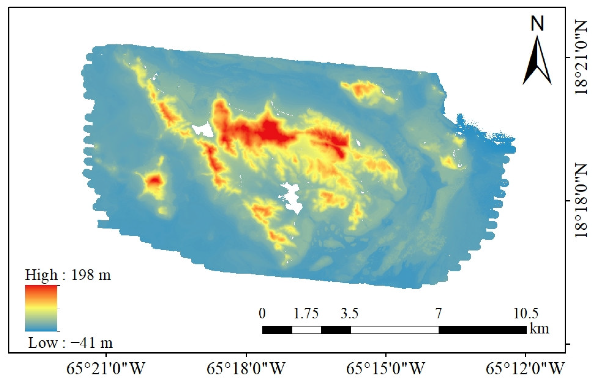
2.1.1. Study Area

The Commonwealth of Puerto Rico is situated in the eastern part of the Greater Antilles in the Caribbean Sea, encompassing the islands of Puerto Rico, Vieques, and Culebra. This study specifically focuses on the Culebra region, which spans from approximately 18.25°N to 18.36°N latitude and 65.15°W to 65.35°W longitude. Figure 1 illustrates images of Culebra and its location, labeled by a red circle.

2.1.2. ICESat-2 ATL03 Data

The study utilized ATL03 data from the study area to validate the proposed bathymetric method and assess its capability. ATL03 data consists of photon point clouds with precise geographic coordinates, capturing geospatial information from signal photons reflected by both the sea surface and seafloor, enabling the reconstruction of ocean profiles and bathymetry.

An ATL03 file comprises six groups of data corresponding to six tracks (gt1l, gt1r, gt2l, gt2r, gt3l, and gt3r, where “l” and “r” represent left and right, respectively). Due to the signal intensity and geographic coordinates, not all groups of data contain distinct signal points of the water bottom. For validation purposes, six ATL03 data with distinct signal points of water bottom were selected from the study area. as depicted in Figure 1, where dashed lines of different colors represent the various ATL03 data tracks.

Table 1. Detailed information of six ATL03 data.

Data Name	Date	Geographic Coordinates Range	Track	Number of LiDAR Points
20190119gt3l	20190119	18.2885°N, 65.2767°W~18.2936°N, 65.2773°W	gt3l	3475
20181024gt3r	20181024	18.3234°N, 65.2391°W~18.3192°N, 65.2395°W	gt3r	4442
20200717gt3l	20200717	18.2965°N, 65.2485°W~18.3001°N, 65.2488°W	gt3l	2450
20200721gt2l	20200721	18.2969°N, 65.2504°W~18.2949°N, 65.2506°W	gt2l	892
20201016gt2l	20201016	18.3290°N, 65.3147°W~18.3316°N, 65.3150°W	gt2l	2063
20190420gt2l	20190420	18.3010°N, 65.3118°W~18.3039°N, 65.3121°W	gt2l	1391

presents detailed information on the six ATL03 data used in this study, including acquisition dates, tracks, geographic coordinates, and the number of LiDAR points.

2.1.3. ALB In Situ Data

In this study, we utilized airborne LiDAR bathymetry data provided by NOAA’s Office of Coastal Management as in situ data for validating the bathymetric accuracy of the ICESat-2 data in our study area. The in situ water depth data were collected on 11 July 2018 by Leading Edge Geomatics using a Riegl VQ-880-G II LiDAR system, as depicted in Figure 2.

2.2. Method

2.2.1. Photon-Counting Bathymetric Method

The ATL03 data obtained from Culebra contain thousands of photon points. Due to the influence of sunlight, water scattering, suspended solids, and other factors, these data include a large number of noise photons in addition to those from the sea surface and seafloor. This noise presents significant challenges for water depth extraction. Therefore, after obtaining the original ATL03 data, the AV-OPTICS model was employed to isolate pure signal photons, including those from the sea surface and seafloor. Subsequently, water depth was extracted based on the coordinates of the signal photons. During this extraction process, it is essential to consider the effects of refraction and tides on the coordinates of the signal photons. Tidal effects cause the sea level to change over time, and the refraction of seawater biases the position of underwater photons. Hence, the influence of both effects on bathymetry must be eliminated to extract the true water depth, which can then be compared with in situ data.

2.2.2. AV-OPTICS Denoising Algorithm

To handle the numerous noise photons in the ATL03 data, the AV-OPTICS model employs an elliptical filter and density threshold to define the distance parameters for each photon. It then screens out noise photons based on the size of these distance parameters. To achieve accurate and automatic denoising, the size of the elliptical filter is adjusted according to the distribution characteristics of the point cloud in different data. The proposed model is divided into three steps to realize this aim, as follows:

(a)

Draw the elevation histogram, perform Gaussian curve fitting, and classify water surface photons and underwater photons based on the confidence interval.

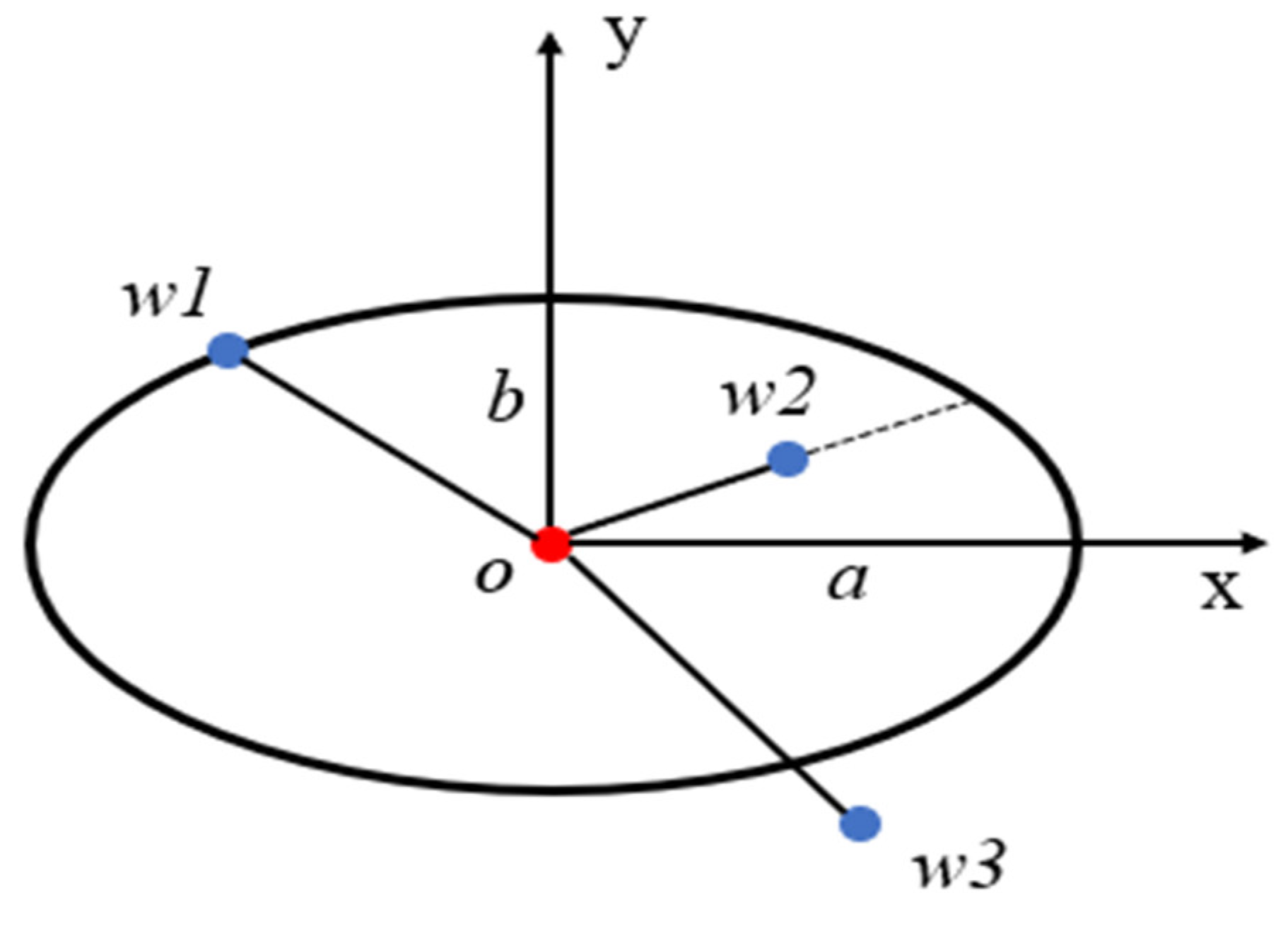
(b)

Calculate the size of the elliptical filter according to the distribution characteristics of underwater photons.

(c)

Use the AV-OPTICS denoising algorithm to extract water bottom photons from underwater photons.

Finally, we integrated the water surface photons obtained in Step (a) with the water bottom photons obtained in Step (c). This enabled the denoising of different ATL03 data and the successful extraction of signal photons.

(a) Based on the elevation distribution of the original photon point cloud data, we obtained a height distribution histogram, as depicted in Figure 3. Two Gaussian peaks were identified by fitting the elevation distribution histogram to a double Gaussian distribution function. According to the characteristics of the ATL03 data, these two peaks correspond to the intervals where the water surface photons and water bottom photons are located. We preliminarily determined the elevation interval with the red profile in Figure 3 corresponding to the water surface photons based on the understanding that the elevation of the water surface is higher than that at the water bottom. We extracted the photons within the 99% confidence interval as water surface photons, while the remaining photons below the intersection of the two Gaussian functions were considered underwater photons.

(b) After obtaining the water surface photons, it is necessary to acquire the water bottom photons from the underwater photons. Owing to the absorption by the water column, signals reflected through the water bottom are much weaker compared to those from the water surface, making extraction more difficult [33]. To accurately extract water bottom photons, [32] applied the OPTICS clustering algorithm to remove noise from underwater photons. The OPTICS algorithm uses an elliptical filter of a certain size to define distribution parameters such as core distance and reach distance for each point, then calculates a reach/distance threshold based on all points in the data. By comparing the reach distance of each point with the reach/distance threshold, it determines whether the point is a signal or a noise point. A detailed introduction to the OPTICS algorithm is in Step (c). However, in the study by [32], the distribution parameters were obtained using a fixed size of the elliptical filter in the OPTICS algorithm, which does not accurately reflect the distribution characteristics of different water bottom terrains in different ATL03 data, resulting in inadequate denoising of photons near the water bottom. To address this limitation, we propose an Adaptive Variable OPTICS (AV-OPTICS) model. This model can calculate more suitable input variables based on the distribution characteristics of the water bottom photons, thereby achieving precise denoising near the bottom of the water.

The input variables of the AV-OPTICS model include the semi-minor axis $b$ and the semi-major axis $a$ of the elliptical filter. The value of $b$ is related to the vertical width of the water bottom contour, whereas the value of $a$ needs to be calculated using the K-means nearest neighbor method.

For different photon cloud data, the photon clouds were concentrated near the water bottom contour, possessing a certain width in the vertical direction, as shown in Figure 4. We measure the vertical width $h$ of the underwater contour and take $h/2$ as the value of $b$. The reason for this is explained in Section 4.1. For relatively flat water bottom terrains, as shown in Figure 4a, the vertical width $h$ of the water bottom contour can be obtained by fitting the elevation distribution histogram with a Gaussian function and then calculating the width of the confidence interval. However, for more complex water bottom terrains, as shown in Figure 4b, where the elevations of the left and right sides are not equal, the elevation distribution histogram may show a bimodal phenomenon, making it difficult to measure the vertical width $h$. To solve this problem, we divided the point cloud data into $n$ segments along the horizontal direction. In this paper, $n$ was set to 11. Each segment’s data could be fitted with a Gaussian function, and the width of the 95% confidence interval was chosen as the value of $h$ for that segment.

To exclude outliers that may be obtained in some segments, the median of the results obtained from multiple segments was taken as the width $h$ of the water bottom contour, and $h/2$ was taken as the value of $b$.

The OPTICS algorithm typically has three input variables: semi-minor axis $b$, semi-major axis $a$, and density threshold $N_{MinPts}$. The density threshold $N_{MinPts}$ can be derived from the semi-minor axis $b$ and semi-major axis $a$, as shown in Equation (1); therefore, it can be considered that the OPTICS algorithm has two input variables: a semi-minor axis $b$ and a semi-major axis $a$.

$$\left\{\begin{array}{l}{S}_1={\displaystyle \frac{\pi ab{N}_1}{h_{1}l}}\\ S_2={\displaystyle \frac{\pi ab{N}_2}{h_{2}l}}\\ N_{MinPts}=ceil[{\displaystyle \frac{2S_1-S_2}{\ln (2S_1/S_2)}}]\end{array}\right.$$

(1)

where $S_1$ denotes the total number of photons within the elliptical filter, $N_1$ represents the total number of photons for a given sample, $h_1$ and $l$ are the maximum differences in the vertical and along-track distances in the photon cloud of the sample, respectively; $S_2$ denotes the number of noise photons within the elliptical filter and $N_2$ is the number of photons within a 5 m range upward from the deepest point and $h_2$ is the height of this range, set to 5 m; $ceil\left(\right)$ represents the ceiling function [34].

From Equation (1), we observe that when $b$ remains constant, the value of $N_{MinPts}$ is a positive integer that correlates positively with $a$. As the value of the semi-minor axis $b$ is already known, the optimal density threshold $N_{MinPts}$ can be determined first, and then $b$ and $N_{\mathrm{M}\mathrm{i}\mathrm{n}\mathrm{P}\mathrm{t}\mathrm{s}}$ can be used to calculate the value of $a$ via backward induction. Compared with $a$, the density threshold $N_{MinPts}$ is one of the parameters that directly influences the denoising effects. An extremely small value of $N_{MinPts}$ results in the retention of more noise points, whereas an excessively large value leads to over-denoising. Regarding the selection of $N_{MinPts}$, research has been conducted indicating that $N_{MinPts}$ are typically fixed at 4 [35]. Therefore, we set the density threshold $N_{MinPts}$ to 4 and then attempted to obtain the value of the semi-major axis $a$ using the known values of the semi-minor axis $b$ and $N_{MinPts}$.

Given the known values of $b$ and $N_{MinPts}$, the K-mean nearest neighbor method [36] was employed to obtain the value of $a$. For data with $n$ points, the K-mean nearest neighbor method involves three steps: (1) compute the distance distribution matrix $D_{nn}$, where $D_{nn}$ is an $n\times n$ symmetric matrix, and $D_{nn}(i,j)$ represents the distance from the $i th$ point to the $j th$ point; (2) sort each row of the distance distribution matrix in ascending order to obtain ${\overline{D}}_{nn}$; (3) calculate the average values of each column of ${\overline{D}}_{nn}$ to obtain the list $D_{es}$. The list $D_{es}$ obtained from the K-nearest neighbor method represents the sorted distances from a certain point $p$ to other points. This study modifies Step (1) to compute a horizontal distance distribution matrix. Consequently, $D_{es}$ obtained after these three steps represents the sorted horizontal distances from a particular point $p$ with the other points. We take these transformed lists $D_{es}$ as the semi-major axis parameter list $D_a$ for $a$, where we choose one as the final value of $a$. Along with the known value of $b$, each value in $D_a$ is substituted into Equation (1) to obtain a density threshold parameter list $D_m$ for $N_{MinPts}$. Based on $D_m$ and $D_a$, we obtained the value of $a$ based on the value of $N_{MinPts}$. However, because of the rounding of $N_{MinPts}$ values in Equation (1), $D_m$ and $D_a$ may include cases where multiple $a$ values correspond to a single $N_{MinPts}$ value. In such instances, the $a$ value corresponding to $N_{MinPts}$ closest to 4 was selected. In other words, the minimum $a$ value when $N_{MinPts}$ is equal to 4 in $D_a$ lists is the final value chosen for the semi-major axis $a$.

In summary, for different underwater scenarios, this study selected half of the vertical width $h$ of the water bottom contour as the value of the semi-minor axis of $b$. Then, employing the K-mean nearest neighbors method, the minimum $a$ value when $N_{\mathrm{M}\mathrm{i}\mathrm{n}\mathrm{P}\mathrm{t}\mathrm{s}}$ was equal to 4, was identified as the value of $a$, achieving automated determination of the input variables.

(c) After obtaining the input variables $b$ and $a$, they were incorporated into the OPTICS algorithm to achieve denoising of underwater photons. Unlike traditional distance metrics, the OPTICS algorithm, based on an elliptical filtering kernel, defines the distance between any two points $p$ and $q$, as shown in Equation (2). In this formula, $x_p$ and $x_q$ represent the along-track distances of points $p$ and $q$; $y_p$ and $y_q$ denote the elevation values of points $p$ and $q$.

$$d(p,q)=\sqrt{{\displaystyle \frac{{(x_p-x_q)}^2}{a^2}}+{\displaystyle \frac{{(y_p-y_q)}^2}{b^2}}}$$

(2)

Under this definition, the distance of the two points is quite different. As shown in Figure 5, point o is the center of the elliptical filter with a semi-minor axis $b$ and a semi-major axis $a$; w1, w2, and w3 are three points near the point p. In these points, w1 is on the elliptical filter, so the distance between w1 and o is 1. w2 is inside the filter, and the distance ow2 is smaller than 1. Similarly, the distance ow3 is greater than 1. Comparing the distance of o and w with 1, we can determine whether a point w is inside the elliptical filter of o or not.

Based on the definition and parameters, the OPTICS algorithm defines two concepts: core distance and reach distance. Within an elliptical filter centered on photon point $p$, if the number of photon points is greater than or equal to the density threshold $N_{MinPts}$, photon point $p$ is identified as the core point. If $p$ is a core point, the minimum distance that makes $p$ a core point is referred to as the core distance of $p$, denoted as $d_c\left(p\right)$. $d_r$ represents the reach distance. If $p$ is a core point, $d_r\left(p,q\right)$ is defined as the maximum distance $d\left(p,q\right)$ between sample point $q$ and core point $p$ or $p$’s core distance $d_c\left(p\right)$. When $p$ was not a core point, $d_r\left(p,q\right)$ were inexistent. The formulas for calculating the core and reach distance are shown in Equations (3) and (4), where $N_{ab}\left(p\right)$ denotes the number of points within an elliptic filter centered on $p$, $a$ and $b$ are the semi-major and semi-minor axes, respectively. $x$ represents a point within the elliptical filter centered on $p$ which is the $N_{MinPts}$th nearest to $p$.

$$d_c(p)=\left\{\begin{array}{l}undefined,N_{ab}(p)<N_{MinPts}\\ d(p,x),N_{ab}(p)\ge N_{MinPts}\end{array}\right.$$

(3)

$$d_r(p,q)=\left\{\begin{array}{l}undefined,N_{ab}(p)<N_{MinPts}\\ \max (d_c(p),d\left(p,q\right)),N_{ab}(p)\ge N_{MinPts}\end{array}\right.$$

(4)

For the photon cloud data, each photon point corresponds to a reach distance $d_r$. A larger $d_r$ indicates a greater distance from other points, whereas a smaller $d_r$ indicates closer proximity to other points. Based on the characteristics of the $d_r$ list, the values of $d_r$ less than 1 were selected and subjected to the OTSU method [37] to obtain the reach/distance threshold $d_{r,th}$. If the reach distance $d_r$ for sample point $p$ is smaller than $d_{r,th}$, then the sample point $p$ is classified as a signal point; otherwise, it is classified as a noise point. This approach effectively separates the signal photon points from the noise photon points based on the reach/distance threshold $d_{r,th}$.

2.2.3. Water Depth Extraction

Based on the aforementioned method, we can obtain pure water surface and bottom signal photons, enabling the extraction of water depth based on these signal photons. However, during the propagation of water bottom photons, both their speed and direction change when they cross the air/water interface. According to Snell’s law, the coordinates of the water bottom photons are shifted due to refraction, which affects the accuracy of water depth extraction. Therefore, it is necessary to perform refraction correction of the water bottom photons during water depth extraction. Simultaneously, sea level periodically changes under the influence of tidal forces from the sun and moon, known as tidal effects. To mitigate the impact of tidal effects on water depth extraction, it is essential to calculate the difference between the instantaneous water level and the reference water level and then obtain water depth values based on the reference water level.

To mitigate these two effects on water depth extraction, we first perform refraction correction to obtain the water depth under instantaneous water level. In this study, we adopted the refraction correction method outlined by [38], which considers the influence of laser incidence angles and water surface fluctuations. Unlike other refraction correction methods, they initially calculate the laser incidence angle $\theta$ using parameters $ref\_elev$ provided by the ATL03 data, as shown in Equation (5). To characterize sea surface fluctuations, a fifth Fourier series was employed to fit the water surface photons. Subsequently, the derivative of the fitted fifth Fourier series is computed to obtain the slope angle $\phi$ of each position on the sea surface, as illustrated in Equation (6). Given the known angles $\theta$ and $\phi$, three conditions are considered, as depicted in Figure 6. By applying Snell’s law and relevant trigonometric principles, the actual positions of the water bottom photons under these three conditions can be determined. Detailed methods for each case are available in the aforementioned paper.

$$\theta ={\displaystyle \frac{\pi }{2}}-ref\_elev$$

(5)

$$\left\{\begin{array}{l}f(x)=a_0+{\displaystyle \sum _{k=1}^5(a_k\cos (k\omega x)+b_k\sin (k\omega x))}\\ \rho (x)={\displaystyle \sum _{k=1}^5(-a_k\omega x\sin (k\omega x)+b_k\omega x\cos (k\omega x))}\\ \phi (x)=\arctan (\rho (x))\end{array}\right.$$

(6)

After refraction correction, we obtained the water depth at the instantaneous water levels. However, owing to tidal effects, the water level varies constantly. Therefore, it was necessary to perform tidal correction to derive the water depth based on the reference water level. This study employed the S-TIDE model [39] for the tidal analysis of the study area to determine the difference between instantaneous and reference water levels. Initially, the equilibrium tide function from the S-TIDE model was used to obtain the height of the equilibrium tide at the detection time, which served as the instantaneous water level in the study area. Simultaneously, mean lower low water (MLLW) was selected as the reference water level for the study area [40]. Centered on the detection time, we utilized the model to predict the equilibrium tide height over a week and then calculated the MLLW during this time, establishing it as the reference water level. After obtaining the instantaneous and reference water levels, the difference $∆h$ between them was calculated. Furthermore, by subtracting $∆h$ from the water depth under instantaneous water level, the water depth based on the reference water level can be obtained. The computational process is detailed in Equations (7)–(9), where $D_{instant}$ and $D_{base}$ represent the water depth under instantaneous water level and reference water level, respectively; $H_{surface\_instant}$, $H_{surfac{e}_{base},}$ and $H_{seafloor}$ represent the elevation of instantaneous water surface, reference water surface, and seafloor, respectively. In ATL03 data, the water surface photons can be moved downward by $∆h$ to characterize the reference water level.

$$D_{instant}=H_{surface\_instant}-H_{seafloor}$$

(7)

$$\Delta h=H_{surface\_instant}-H_{surface\_base}$$

(8)

$$D_{base}=H_{surface\_base}-H_{seafloor}=D_{instant}-\Delta h$$

(9)

After applying refraction and tide corrections, we employed a fifth-order Fourier series to model the water surface elevation from the photon data. The average value of this series was then taken as the relative elevation of the water surface. For deriving the water bottom profile, we utilized a B-spline to fit the photon data from the water bottom. Finally, we extracted water depths according to the height difference between the water surface and water bottom and validated these bathymetric values by comparing them with in situ data.

3. Results

3.1. Evaluation Methodology

To validate the accuracy of the AV-OPTICS model, six sets of point cloud data were extracted from the ATL03 data, as described in Section 2.1.2. The experiments evaluated the model’s performance in terms of denoising and bathymetric accuracy. The denoising effect of the model was assessed using the $F1$ value and cohesion $C_{oh}$, whereas the bathymetric accuracy was evaluated using the mean absolute error ($MAE$) and root mean square error ($RMSE$).

To assess the denoising effectiveness of the AV-OPTICS model, we employed two metrics: the $F1$ score to gauge overall performance and cohesion $C_{oh}$ for a detailed assessment.

The $F1$ score, widely utilized in point-cloud classification, is derived from the weighted harmonic average of Recall $R$ and Precision $P$, as illustrated in Equation (10). $N_{TP}$ denotes the number of correctly classified signal photons, $N_{FN}$ is the number of incorrectly classified signal photons and $N_{FP}$ is the number of incorrectly classified noise photons. A higher $F1$ value indicates better overall denoising performance of the model.

$$\left\{\begin{array}{l}F1={\displaystyle \frac{2\times P\times R}{P+R}}\\ P={\displaystyle \frac{N_{TP}}{N_{TP}+N_{FP}}}\\ R={\displaystyle \frac{N_{TP}}{N_{TP}+N_{FN}}}\end{array}\right.$$

(10)

Cohesion $C_{oh}$ reflects the extent of point-cloud dispersion within a certain region and measures the denoising effect. A smaller cohesion value indicated fewer discrete noise points within this region. The formula for cohesion is shown in Equation (11), where $C_{oh}$ represents the value of cohesion, $r$ denotes the number of photon points within a specific region, $x_i$ indicates the photon points within the region, $c$ refers to the centroid within the region, and $proximity\left(\right)$ denotes the proximity formula used to compute the proximity between the two points.

$$C_{oh}={\displaystyle \sum _{i=1}^{r}proximity(x_i,c)}$$

(11)

Typically, the proximity formula is based on the squared Euclidean distance. However, considering that the noise points are vertically distributed near the water bottom contour, the vertical distance is more relevant to the denoising effect. Therefore, this study adopted the squared vertical distance as the formula for proximity, with the centroid position being the average vertical distance of all points within the region.

To evaluate the bathymetric accuracy of the AV-OPTICS model, this study employed two evaluation indexes: $MAE$ and $RMSE$. $MAE$ is the mean absolute error between bathymetric and in situ data, providing an intuitive observation of the error. $MAE$ can be used to evaluate the overall bathymetric accuracy of the model. $RMSE$ is the root mean square error between the bathymetric and in situ data, which is more sensitive to outliers in bathymetry data compared to $MAE$, making it a more effective metric for discerning subtle differences between different models. As such, we utilized $RMSE$ to compare the performance of various bathymetry models. The formulae for $MAE$ and $RMSE$ calculations are shown in Equations (12) and (13). In the two Equations, $y_i$ represents the value of bathymetric data obtained by the model, $\widehat{y_i}$ denotes the value of in situ data, $n$ indicates the number of data points.

$$MAE={\displaystyle \frac{1}{n}}{\displaystyle \sum _{i=1}^n|y_i-\widehat{y_i}|}$$

(12)

$$RMSE=\sqrt{{\displaystyle \frac{1}{n}}{\displaystyle \sum _{i=1}^n{(y_i-\widehat{y_i})}^2}}$$

(13)

3.2. Denoising Results and Comparison

The AV-OPTICS model automatically calculates input variables based on photon distribution characteristics to denoise raw photons and extract water surface and bottom photons precisely. In this study, we selected six ATL03 data from the Culebra region; among them, three data are illustrated in Figure 7a,d,g. Denoising results using the AV-OPTICS model are presented in Figure 7b,e,h, where the water surface, bottom, and noise photons are annotated with blue, red, and grey points, respectively. Figure 7b,e,h demonstrate the AV-OPTICS model’s effectiveness in denoising and extracting water surface and bottom photons from the raw photons.

To demonstrate the advantages of the AV-OPTICS model, we conducted a comparative experiment using the traditional OPTICS algorithm, which employs fixed input variables determined via trial and error [32]. The denoising results of the traditional OPTICS model are shown in Figure 7c,f,i. Both methods exhibit effective denoising in regions distant from the water bottom, as depicted in Figure 7. However, near the water bottom, the AV-OPTICS model shows fewer noise photon points compared to the traditional OPTICS algorithm. To quantitatively compare the two methods, the $F1$ value and $C_{oh}$ were computed for each method.

Based on the manually annotated signal photons, the $F1$ values for the different ATL03 data were calculated using Equation (10), and the results are listed in

Table 2. $F1$-score, $P,$ and $R$ of our method and traditional OPTICS.

Data Name	Our Method			Traditional OPTICS
	$\mathit{F}1$-Score	$\mathit{P}$	$\mathit{R}$	$\mathit{F}1$-Score	$\mathit{P}$	$\mathit{R}$
20190119gt3l	0.9704	0.9559	0.9854	0.9635	0.9310	0.9983
20181024gt3r	0.9885	0.9901	0.9870	0.9850	0.9781	0.9921
20200717gt3l	0.9631	0.9888	0.9388	0.9594	0.9203	1.0000
20200721gt2l	0.9722	0.9633	0.9813	0.9664	0.9328	1.0000
20201016gt2l	0.9740	0.9717	0.9779	0.9652	0.9476	0.9833
20190420gt2l	0.9837	0.9809	0.9865	0.9740	0.9545	0.9944
Average value	0.9753	0.9751	0.9762	0.9689	0.9441	0.9947

. Table 2 shows six sets of $F1$ values corresponding to the denoising outcomes. The average $F1$ value achieved by our AV-OPTICS algorithm is 97.53%, while the average $F1$ value obtained by the traditional OPTICS algorithm is 96.89%. This comparison indicates that the AV-OPTICS model offers an improvement in denoising accuracy compared to the traditional OPTICS model.

Combined with the observations in the previous paragraph, the AV-OPTICS model notably improves denoising accuracy, especially in areas near the water bottom.

To further emphasize the advantages of AV-OPTICS in the vicinity of water bottoms, it is crucial to magnify the contours of the water bottoms and conduct a detailed comparison between the two models. Specifically, we examined the data named 20181024gt3r and 20190420gt2l. The enlarged water bottom contours are depicted in Figure 8, highlighting that our algorithm produces fewer noise points near the water bottom in both experimental scenarios. To quantitatively reflect this observation, we applied Equation (11) to compute the cohesion of photons within the black boxes shown in Figure 8. The results are summarized in

Table 3. Cohesion values of our method and traditional OPTICS within the selected region.

Data Name	Selected Region		Cohesion
	x [m]	y [m]	Our Method	Traditional OPTICS
20190119gt3l	2.03308 × 106~2.03315 × 106	−50~−46	63.31	87.74
20181024gt3r	1.80346 × 107~1.80347 × 107	−50~−46	19.52	28.60
20200717gt3l	2.03345 × 106~2.03355 × 106	−49~−43	17.86	41.39
20200721gt2l	1.80376 × 107~1.80377 × 107	−48~−43	5.81	13.87
20201016gt2l	2.03760 × 106~2.03765 × 106	−52~−45	36.52	50.90
20190420gt2l	2.03455 × 106~2.03466 × 106	−54~−49	5.77	13.87
Average value			24.80	39.40

.

According to Table 3, in the vicinity of the water bottom, our method achieved an average cohesion of 24.80 m², whereas the traditional OPTICS algorithm recorded an average cohesion of 39.40 m². These findings indicate that our method achieves lower average cohesion and fewer noise points near the water bottom compared to the traditional OPTICS method.

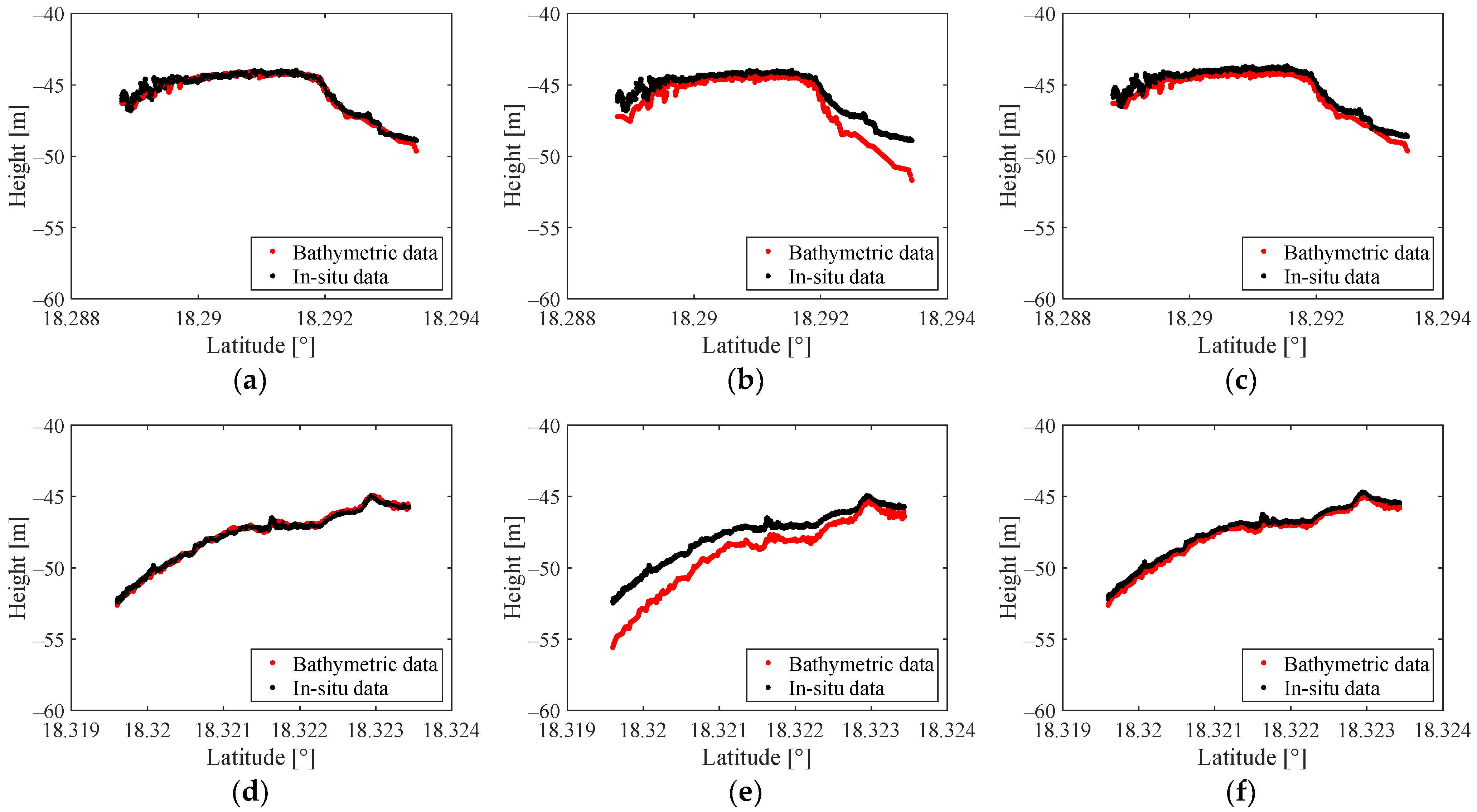
3.3. Bathymetric Accuracy and Comparison

To enhance bathymetric accuracy, it is crucial to perform coordinate correction of photons during water depth extraction to mitigate the effects of refraction and tides. Using 20190119gt3l and 20181024gt3r as examples, coordinate correction was conducted following the methodology outlined in Section 2.2.3, and the results are illustrated in Figure 9.

In Figure 9, the original coordinates of the surface and bottom photons are denoted by blue and red dots, respectively. Corrected coordinates after photon correction for surface and bottom photons are indicated by purple and green dots, respectively. Figure 9a,c demonstrate that the actual positions of water bottom photons are higher than their original positions due to the refraction of the seawater. Furthermore, the deeper the water, the greater the deviation between actual and original positions. Conversely, as shown in Figure 9a,c, the corrected positions of water surface photons were lower than their original positions. This adjustment aligns with the study area’s reference water level, which is typically MLLW (Mean Lower Low Water); hence, instantaneous water levels are typically higher than this reference. Therefore, water surface photons were adjusted downward to the relative position of the reference water level to derive water depth data based on this standard. Following refraction and tidal corrections, a fitting procedure was employed to extract depth information from both water surface and bottom photons, as depicted in Figure 9b,d, respectively. Profiles of the water bottom and reference water surface are represented by black and blue lines, respectively, with detailed fitting methods explained in Section 2.2.3.

Using the aforementioned method, we successfully extracted bathymetric data from the ATL03 data. To validate their bathymetric accuracy, we utilized ALB data introduced in Section 2.1.3 as in situ data for verifying the bathymetric results obtained via photon-counting LiDAR. Taking data 20190119gt3l and 20190420gt2l as examples, a comparison between bathymetric data and in situ data is illustrated in Figure 10a,c, where the red and black points represent bathymetric and in situ data, respectively. From Figure 10a,c, it is evident that the water bottom profiles derived from the bathymetric data closely match the in situ data profiles. Concurrently, comparative experiments were conducted using the traditional OPTICS algorithm, as shown in Figure 10b,d. Comparing Figure 10a,c with 10b,d, it is observable that the water bottom profiles obtained using the traditional OPTICS method exhibit deviations from the in situ data in certain areas, primarily due to noise points near the water bottom. To further elucidate this observation, we quantitatively compared the bathymetric accuracy of both methods using $MAE$ and $RMSE$. The results of this comparison are presented in

Table 4. $MAE$ and $RMSE$ of our method and traditional OPTICS.

Data Name	Our Method		Traditional OPTICS
	$\mathit{M}\mathit{A}\mathit{E}$	$\mathit{R}\mathit{M}\mathit{S}\mathit{E}$	$\mathit{M}\mathit{A}\mathit{E}$	$\mathit{R}\mathit{M}\mathit{S}\mathit{E}$
20190119gt3l	0.17	0.24	0.27	0.41
20181024gt3r	0.10	0.13	0.11	0.15
20200717gt3l	0.28	0.33	0.31	0.41
20200721gt2l	0.49	0.51	0.55	0.56
20201016gt2l	0.29	0.33	0.34	0.42
20190420gt2l	0.32	0.34	0.38	0.43
Average value	0.28	0.31	0.33	0.40

.

Using the ALB data from Section 2.1.3 as the in situ reference in Table 4, the $MAE$ of the bathymetric data obtained by our method ranges between 0.10 m and 0.49 m, averaging 0.28 m, while the $RMSE$ ranges from 0.13 m to 0.51 m, averaging 0.31 m. From the six ATL03 data, 20181024gt3r has the lowest $MAE$ and $RMSE$ while 20181024gt3r has the highest. That is probably related to the LiDAR point number of the data. Combining with Table 1, we can find the ATL03 data with more photon points has lower $MAE$ and $RMSE$ in most cases, which also means the data with stronger signal intensity are more likely to have a better bathymetric result. In comparison, the $MAE$ ranges from 0.11 m to 0.55 m, averaging 0.33 m, with $RMSE$ values of the bathymetric data obtained by traditional OPTICS model ranging from 0.15 m to 0.56 m and averaging 0.40 m. Our method achieves lower $MAE$ and $RMSE$ values compared to the traditional OPTICS model. Specifically, our method reduces the average $MAE$ by 0.05 m and the average $RMSE$ by 0.09 m. This demonstrates that our method provides bathymetric data with smaller errors relative to the in situ data, indicating higher accuracy compared to the traditional OPTICS model.

4. Discussion

4.1. The Parameters of AV-OPTICS

In Section 3.2, it was established that the AV-OPTICS model outperformed the traditional OPTICS model in denoising near the water bottom. This section aims to explore the underlying reasons by analyzing two key input variables: the semi-minor axis $b$ and the semi-major axis $a$ of the elliptical filter. Under ideal conditions, a specific contour of water bottom photons can be approximated as a rectangle. When considering the elliptical filter without horizontal dimension consideration, it resembles a vertical line segment of length $2b$, as illustrated in Figure 11.

In Figure 11, if the vertical width of the water bottom contour is denoted as $h$, the points outside this range are considered as noise points. Identified point $p1$ as a noise point, when the semi-minor axis $b>h$, the number of points within the idealized elliptical filter centered on $p1$ is approximately equal to the number of points within the idealized elliptical filter centered on $q1$, which is the central point of the water bottom contour. This implies that the distribution densities of points $p1$ and $q1$ are similar, making $p1$ less likely to be removed as a noise point. To effectively remove $p1$, it is necessary to reduce the value of $b$. When the semi-minor axis $b$ decreases to $h$, the number of points within the idealized elliptical filter centered on edge point $p2$ of the water bottom contour is approximately equal to the number of points within the ideal elliptical filter centered on $q2$, which is the central point of the water bottom contour. However, given the elevation distribution of the water bottom contour, which resembles a Gaussian distribution, it is unreasonable to assume identical density distributions between the edge and central points. According to Equation (1), when $b$ is too small, the density threshold $N_{MinPts}$ becomes extremely low, leaving many discrete noise points that do not satisfy the requirements. From the above analysis, it can be concluded that the value of the semi-minor axis $b$ should be in the range of 0 to $h$. However, the values at the extremes of this range are not suitable. Therefore, a compromise was achieved by setting $b=h/2$.

Similar to the analysis of the semi-minor axis, considering the detailed parts of the water bottom contour as a rectangle and neglecting the vertical distance of the elliptical filter, the ellipse can be simplified as a horizontal line segment of length $2a$. The horizontal direction of the idealized model is depicted in Figure 12.

Based on the above analysis, if point $q1$ is a noise point and the length of the yellow segment equals to $2a$, the distribution densities of points $q1$ and central points $q2$ are similar, and both $q1$ and the central point $q2$ are treated as noise points and removed, resulting in the disappearance of the water bottom details on both sides. Conversely, if point $q3$ is a noise point and $2a$ is shortened to the length of the red segment, the neighborhood density around noise point $q3$ and detail center $q4$ will differ, allowing $q4$ to be preserved while $q3$ is removed. However, when the value of $a$ is too low, it causes $N_{MinPts}$ to be extremely small, resulting in the retention of more discrete noise points. From this analysis, it is evident that maintaining the semi-minor axis $b$ a constant and increasing the semi-major axis $a$ leads to fewer discrete noise points but may sacrifice some water bottom details on both sides. Conversely, decreasing $a$ preserves the water bottom details on both sides but allows more discrete noise points to persist. Therefore, the selection of a should balance the preservation of terrain details on both sides and minimize discrete noise points. Based on the theoretical basis of Section 2.2.2, the minimum value of $a$ when $N_{MinPts}=4$ is chosen as the semi-major axis to minimize discrete noise points while preserving water bottom details on both sides as far as possible.

Based on this analysis, we can elucidate the denoising effects of the AV-OPTICS model compared to the traditional OPTICS algorithm. In various experimental scenarios, the semi-minor $b$ in the traditional OPTICS algorithm was approximately or more than twice the value obtained automatically using our method. As discussed, an excessively large value of $b$ can result in noise photons near the water bottom having similar distribution densities to the water bottom signal photons at the contour’s center, posing challenges for differentiation. This adversely impacts the denoising efficacy in the vicinity of the water bottom. Overall, compromised denoising near the water bottom affects precision $P$, resulting in decreased $F1$ values and impacting overall denoising accuracy.

4.2. Error Analysis of Bathymetry

To further demonstrate the enhanced bathymetry performance of our method, in this section, we use two data, 20190119gt3l and 20201016gt2l, as examples and assess the errors between the bathymetric data points obtained by both methods and the in situ data points by plotting error distribution histograms, as depicted in Figure 13. In these figures, the x-axis represents the error values between the bathymetric data and in situ data with an interval of 0.5 m, while the y-axis denotes the percentage of points corresponding to each error value. Figure 13a,c show the error statistics for the AV-OPTICS model, whereas Figure 13b,d indicate those for the traditional OPTICS method. From the graphs, it is evident that our method yields depth errors predominantly within the range of −1 m to 1 m, with approximately 90% of errors having an absolute value within 0.5 m. In contrast, the traditional OPTICS method shows a wider distribution range of depth errors, with fewer errors having an absolute value within 0.5 m compared to the AV-OPTICS model.

To better evaluate the error distribution, we calculated the percentages of depth errors within the intervals [−1 m, 1 m] and [−0.5 m, 0.5 m] for six data under each method, summarized in

Table 5. Proportion of error distribution of our method and traditional OPTICS.

Data Name	Our Method		Traditional OPTICS
	Proportion of [−1, 1]	Proportion of [−0.5, 0.5]	Proportion of [−1, 1]	Proportion of [−0.5, 0.5]
20190119gt3l	0.9974	0.9420	0.9574	0.8308
20181024gt3r	1.0000	0.9995	1.0000	0.9952
20200717gt3l	0.9923	0.8866	0.9829	0.8504
20200721gt2l	0.9991	0.4004	0.9951	0.3507
20201016gt2l	1.0000	0.8915	0.9786	0.7791
20190420gt2l	1.0000	0.8885	0.9867	0.7987
Average value	0.9981	0.8348	0.9835	0.7675

. According to Table 5, our method shows that nearly all errors fall within the [−1 m, 1 m] range, with an average percentage of 99.81%. Within the narrower range of [−0.5 m, 0.5 m], the average percentage is 83.48%. In contrast, the traditional OPTICS algorithm averages 98.35% of errors within the [−1 m, 1 m] range and 76.75% within the [−0.5 m, 0.5 m] range. These percentages are lower compared to our method. This indicates that our method offers improved detection performance and bathymetric accuracy relative to the traditional OPTICS algorithm. This improvement stems from the AV-OPTICS model’s effective denoising near the water bottom, which reduces the impact of nearby noise photons on the water bottom profile, thereby concentrating the error distribution and minimizing depth measurement deviations.

4.3. Influence of Other Factors on Bathymetry

Throughout the bathymetry process, in addition to the AV-OPTICS model, two critical processes were employed: refraction correction and tidal correction. This section investigates their impact on bathymetric accuracy using 20190119gt3l and 20181024gt3r as examples. Firstly, without refraction correction, the bathymetric data are illustrated in Figure 14b,e. These figures reveal a significant decrease in bathymetric accuracy compared to the complete process, particularly with larger deviations as water depth increases. Similarly, omitting tidal correction throughout the process yields results shown in Figure 14c,f. Here, the absence of tidal correction causes a slight downward shift in the water bottom profile compared to the complete process, leading to decreased bathymetric accuracy. The detailed evaluation indices are listed in

Table 6. $MAE$ and $RMSE$ of our method compared with the work without coordinate correction.

Data Name	Our Method		Our Method without Refraction Correction		Our Method without Tide Correction
	$\mathit{M}\mathit{A}\mathit{E}$	$\mathit{R}\mathit{M}\mathit{S}\mathit{E}$	$\mathit{M}\mathit{A}\mathit{E}$	$\mathit{R}\mathit{M}\mathit{S}\mathit{E}$	$\mathit{M}\mathit{A}\mathit{E}$	$\mathit{R}\mathit{M}\mathit{S}\mathit{E}$
20190119gt3l	0.17	0.24	0.85	1.05	0.39	0.45
20181024gt3r	0.10	0.13	1.46	1.63	0.25	0.28
20200717gt3l	0.28	0.33	0.43	0.54	0.29	0.34
20200721gt2l	0.49	0.51	1.19	1.21	0.50	0.52
20201016gt2l	0.29	0.33	1.68	1.83	0.33	0.38
20190420gt2l	0.32	0.34	2.19	2.20	0.32	0.34
Average value	0.28	0.31	1.30	1.41	0.35	0.39

.

The observations from Figure 14 and the evaluation indices in Table 6 indicate that both refraction correction and tidal correction influence the bathymetric accuracy. Among them, refraction correction had a greater impact, with deviations increasing as the water depth increased. To determine the reasons for this, we observed the magnitudes of the depth variations induced by each process. According to calculations from the S-TIDE model, tidal correction results in depth variations of approximately 0.2 m across the six data. Conversely, refraction correction, governed by Snell’s law, leads to depth variations roughly 0.25 times the original water depth, increasing proportionally with depth. For data with mean depths approximately equal to 4 m, the influence of refraction correction on $MAE$ and $RMSE$ values of bathymetric data is on the order of 10⁰ m, whereas tidal correction impacts $MAE$ and $RMSE$ values on the order of 10⁻¹ m. Therefore, the magnitude of depth variations caused by these correction processes significantly affects bathymetric accuracy.

5. Conclusions

This study presents a photon-counting LiDAR bathymetry method based on the Adaptive Variable OPTICS (AV-OPTICS) model. Unlike traditional OPTICS methods with fixed input variables, this approach automatically calculates the input variables based on point cloud distribution. This adjustment ensures precise measurement of photon distribution parameters near the water bottom, thereby enhancing denoising effects in these areas and improving bathymetric accuracy. Experimental validation using ATL03 photon data from Culebra Island, Puerto Rico, demonstrates better denoising performance compared to traditional OPTICS methods, reflected in higher $F1$-values and lower cohesion. Using ALB data as in situ reference, our method achieves an average $MAE$ of 0.28 m and $RMSE$ of 0.31 m, indicating better bathymetric accuracy than traditional OPTICS methods. This study establishes a robust framework for shallow-water bathymetry based on photon-counting LiDAR. Future research will integrate our AV-OPTICS method with satellite remote sensing images for comprehensive 3D mapping of underwater landscapes.

References

1. Li, Y.; Zhou, X.; Li, G.; Guo, J.; Ma, Y.; Chen, Y. Progress and Prospect of Space-borne Photon-counting Lidar Shallow Water Bathymetry Technology. Infrared Laser Eng. 2022, 51, 107–116. Available online: https://kns.cnki.net/kcms/detail/12.1261.TN.20220310.1926.005.html (accessed on 2 February 2024).
2. Nicholls, R.J.; Cazenave, A. Sea-level rise and its impact on Coastal Zones. Science 2010, 328, 1517–1520. [Google Scholar] [CrossRef] [PubMed]
3. Wang, Y.; Zhang, J.; Zheng, Y.; Xu, Y.; Xu, J.; Jiao, J.; Su, Y.; Lv, H.; Liang, K. Brillouin scattering spectrum for liquid detection and applications in oceanography. Opto-Electron. Adv. 2023, 6, 43–53. [Google Scholar] [CrossRef]
4. Wang, B.; Ma, Y.; Zhang, J.; Zhang, H.; Zhu, H.; Leng, Z.; Zhang, X.; Cui, A. Noise Removal Algorithm Based on Adaptive Elevation Difference Thresholding for ICESat-2 Photon-counting Data. Int. J. Appl. Earth Obs. Geoinf. 2023, 117, 103207. [Google Scholar] [CrossRef]
5. Janowski, L.; Trzcinska, K.; Tegowski, J.; Kruss, A.; Rucinska-Zjadacz, M.; Pocwiardowski, P. Nearshore Benthic Habitat Mapping Based on Multi-Frequency, Multibeam Echosounder Data Using a Combined Object-Based Approach: A Case Study from the Rowy Site in the Southern Baltic Sea. Remote Sens. 2018, 10, 1983. [Google Scholar] [CrossRef]
6. Martí, A.; Portell, J.; Amblas, D.; de Cabrera, F.; Vilà, M.; Riba, J.; Mitchell, G. Compression of Multibeam Echosounders Bathymetry and Water Column Data. Remote Sens. 2022, 14, 2063. [Google Scholar] [CrossRef]
7. Casal, G.; Harris, P.; Monteys, X.; Hedley, J.; Cahalane, C.; McCarthy, T. Understanding satellite-derived bathymetry using sentinel 2 imagery and spatial prediction models. GISci. Remote Sens. 2020, 57, 271–286. [Google Scholar] [CrossRef]
8. Wright, C.W.; Kranenburg, C.; Battista, T.A.; Parrish, C. Depth calibration and validation of the Experimental Advanced Airborne Research Lidar, EAARL-B. J. Coast. Res. 2016, 76, 4–17. [Google Scholar] [CrossRef]
9. Zhao, Y.; Wang, Y.; Liang, K.; Xu, Y.; Guo, Y.; Makame, K. Underwater Temperature and Salinity Measurement by Rayleigh–Brillouin Spectroscopy Using Fizeau Interferometer and PMT Array. Remote Sens. 2024, 16, 2214. [Google Scholar] [CrossRef]
10. Renga, A.; Rufino, G.; D’Errico, M.; Moccia, A.; Boccia, V.; Graziano, M.D.; Aragno, C.; Zoffoli, S. SAR bathymetry in the Tyrrhenian Sea by COSMO-SkyMed data: A novel approach. IEEE J. Sel. Top. Appl. Earth Obs. Remote Sens. 2014, 7, 2834–2847. [Google Scholar] [CrossRef]
11. He, J.; Xu, Y.; Sun, H.; Jiang, Q.; Yang, L.; Kong, W.; Liu, Y. Sea Surface Height Wavenumber Spectrum from Airborne Interferometric Radar Altimeter. Remote Sens. 2024, 16, 1359. [Google Scholar] [CrossRef]
12. Parrish, C.E.; Magruder, L.A.; Neuenschwander, A.L.; Forfinski-Sarkozi, N.; Alonzo, M.; Jasinski, M. Validation of ICESat-2 ATLAS Bathymetry and Analysis of ATLAS’s Bathymetric Mapping Performance. Remote Sens. 2019, 11, 1634. [Google Scholar] [CrossRef]
13. Kutser, T.; Hedley, J.; Giardino, C.; Roelfsema, C.; Brando, V.E. Remote sensing of shallow waters—A 50 year retrospective and future directions. Remote Sens. Environ. 2020, 240, 111619. [Google Scholar] [CrossRef]
14. Magruder, L.A.; Brunt, K.M. Performance Analysis of Airborne Photon- Counting Lidar Data in Preparation for the ICESat-2 Mission. IEEE Trans. Geosci. Remote Sens. 2018, 56, 2911–2918. [Google Scholar] [CrossRef]
15. Xie, J.; Zhong, J.; Mo, F.; Liu, R.; Li, X.; Yang, X.; Zeng, J. Denoising and Accuracy Evaluation of ICESat-2/ATLAS Photon Data for Nearshore Waters Based on Improved Local Distance Statistics. Remote Sens. 2023, 15, 2828. [Google Scholar] [CrossRef]
16. Markus, T.; Neumann, T.; Martino, A.; Abdalati, W.; Brunt, K.; Csatho, B.; Farrell, S.; Fricker, H.; Gardner, A.; Harding, D.; et al. The Ice, Cloud, and land Elevation Satellite-2 (ICESat-2): Science requirements, concept, and implementation. Remote Sens. Environ. 2017, 190, 260–273. [Google Scholar] [CrossRef]
17. Magruder, L.A.; Wharton, M.E., III; Stout, K.D.; Neuenschwander, A.L. Noise filtering techniques for photon-counting ladar data. In Proceedings of the SPIE 8379, Laser Radar Technology and Applications XVII, Baltimore, MD, USA, 24–26 April 2012; Volume 83790Q, p. 83790Q. [Google Scholar] [CrossRef]
18. Neumann, T.A.; Martino, A.J.; Markus, T.; Bae, S.; Bock, M.R.; Brenner, A.C.; Brunt, K.M.; Cavanaugh, J.; Fernandes, S.T.; Hancock, D.W.; et al. The ice, cloud, and Land Elevation Satellite—2 mission: A global geolocated photon product derived from the Advanced Topographic Laser Altimeter System. Remote Sens. Environ. 2019, 233, 111325. [Google Scholar] [CrossRef]
19. Brunt, K.M.; Neumann, T.A.; Walsh, K.M.; Markus, T. Determination of local slope on the Greenland ice sheet using a multibeam photon-counting lidar in preparation for the ICESAT-2 Mission. IEEE Geosci. Remote Sens. Lett. 2014, 11, 935–939. [Google Scholar] [CrossRef]
20. Chen, B.; Pang, Y. A denoising approach for detection of canopy and ground from ICESat-2’s airborne simulator data in Maryland, USA. In Proceedings of the SPIE 9671, AOPC 2015: Advances in Laser Technology and Applications, Beijing, China, 5–7 May 2015; Volume 96711S, p. 96711S. [Google Scholar] [CrossRef]
21. Moussavi, M.S.; Abdalati, W.; Scambos, T.; Neuenschwander, A. Applicability of an automatic surface detection approach to micro-pulse photon-counting lidar altimetry data: Implications for canopy height retrieval from future ICESat-2 data. Int. J. Remote Sens. 2014, 35, 5263–5279. [Google Scholar] [CrossRef]
22. Chen, Y.; Le, Y.; Zhang, D.; Wang, Y.; Qiu, Z.; Wang, L. A photon-counting LiDAR bathymetric method based on adaptive variable ellipse filtering. Remote Sens. Environ. 2021, 256, 112326. [Google Scholar] [CrossRef]
23. Zhang, W.; Xu, N.; Ma, Y.; Yang, B.; Zhang, Z.; Wang, X.H.; Li, S. A maximum bathymetric depth model to simulate satellite photon-counting lidar performance. ISPRS J. Photogramm. Remote Sens. 2021, 174, 182–197. [Google Scholar] [CrossRef]
24. Ma, Y.; Xu, N.; Liu, Z.; Yang, B.; Yang, F.; Wang, X.H.; Li, S. Satellite-derived bathymetry using the ICESat-2 lidar and Sentinel-2 imagery datasets. Remote Sens. Environ. 2020, 250, 112047. [Google Scholar] [CrossRef]
25. Babbel, B.J.; Parrish, C.E.; Magruder, L.A. ICESat-2 Elevation Retrievals in Support of Satellite-Derived Bathymetry for Global Science Applications. Geophys. Res. Lett. 2021, 48, e2020GL090629. [Google Scholar] [CrossRef] [PubMed]
26. Zhu, X.; Nie, S.; Wang, C.; Xi, X.; Wang, J.; Li, D.; Zhou, H. A noise removal algorithm based on OPTICS for Photon-Counting LiDAR Data. IEEE Geosci. Remote Sens. Lett. 2021, 18, 1471–1475. [Google Scholar] [CrossRef]
27. Wang, X.; Pan, Z.; Glennie, C. A novel noise filtering model for photon-counting laser altimeter data. IEEE Geosci. Remote Sens. Lett. 2016, 13, 947–951. [Google Scholar] [CrossRef]
28. Zhang, J.; Kerekes, J.; Csatho, B.; Schenk, T.; Wheelwright, R. A clustering approach for detection of ground in micropulse photon-counting LiDAR altimeter data. In Proceedings of the IEEE Geoscience and Remote Sensing Symposium, Quebec City, QC, Canada, 13–18 July 2014; pp. 177–180. [Google Scholar] [CrossRef]
29. Ankerst, M.; Breunig, M.M.; Kriegel, H.P.; Sander, J. OPTICS: Ordering points to identify the clustering structure. ACM SIGMOD Rec. 1999, 28, 49–60. [Google Scholar] [CrossRef]
30. Febriana, L.N.; Sitanggang, S.I. Outlier Detection on Hotspot Data in Riau Province using OPTICS Algorithm. IOP Conf. Ser. Earth Environ. Sci. 2017, 58, 012004. [Google Scholar] [CrossRef]
31. Zhang, S.; Zhang, S.; Qiao, N.; Wang, Y.; Du, Q. Modelling and Mitigating Wind Turbine Clutter in Space–Air Bistatic Radar. Remote Sens. 2024, 16, 2674. [Google Scholar] [CrossRef]
32. Xi, X.; Wang, Z.; Wang, C. Bathymetric Extraction Method of Nearshore Based on ICESat-2/ATLAS Data. J. Tongji Univ. (Nat. Sci.) 2022, 50, 940–946. [Google Scholar] [CrossRef]
33. Jia, K.; Ma, Y.; Zhang, J.; Wang, B.; Zhang, X.; Cui, A. A Denoising Methodology for Detecting ICESat-2 Bathymetry Photons Based on Quasi Full Waveform. IEEE Trans. Geosci. Remote Sens. 2024, 62, 4207916. [Google Scholar] [CrossRef]
34. Ma, Y.; Xu, N.; Sun, J.; Wang, X.H.; Yang, F.; Li, S. Estimating water levels and volumes of lakes dated back to the 1980s using Landsat imagery and photon-counting lidar datasets. Remote Sens. Environ. 2019, 232, 111287. [Google Scholar] [CrossRef]
35. Yue, S.; Li, P.; Guo, J.; Zhou, S. A statistical information-based clustering approach in distance space. J. Zhejiang Univ. Sci. A (Sci. Eng.) 2005, 01, 72–79. [Google Scholar] [CrossRef]
36. Saputra, M.E.; Mawengkang, H.; Nababan, E.B. Determination value K in K-nearest neighbor with local mean euclidean and weight Gini Index. IOP Conf. Ser. Mater. Sci. Eng. 2018, 420, 012098. [Google Scholar] [CrossRef]
37. Khambampati, A.K.; Liu, D.; Konki, S.K.; Kim, K.Y. An automatic detection of the ROI using otsu Thresholding in Nonlinear Difference Eit Imaging. IEEE Sens. J. 2018, 18, 5133–5142. [Google Scholar] [CrossRef]
38. Chen, L.; Xing, S.; Zhang, G.; Guo, S.; Gao, M. Refraction Correction Based on ATL03 Photon Parameter Tracking for Improving ICESat-2 Bathymetry Accuracy. Remote Sens. 2024, 16, 84. [Google Scholar] [CrossRef]
39. Pan, H.; Lv, X.; Wang, Y.; Matte, P.; Chen, H.; Jin, G. Exploration of tidal-fluvial interaction in the Columbia River estuary using S_TIDE. J. Geophys. Res. Ocean. 2018, 123, 6598–6619. [Google Scholar] [CrossRef]
40. Hess, K.W. Tidal Datums and Tide Coordination. J. Coast. Res. 2003, 38, 33–43. Available online: http://www.jstor.org/stable/25736598 (accessed on 20 May 2024).
Figure 1. Study area and the detection tracks of ATLAS represented by six different colors of dashed lines.
Remotesensing 16 03438 g001
Figure 2. Water depth results of study area for ALB reference data.
Remotesensing 16 03438 g002
Figure 3. The elevation distribution histogram of ATL03 photon data.
Remotesensing 16 03438 g003
Figure 4. The contours of the water bottom terrain under different scenarios. (a) relatively flat water bottom terrains; (b) complex water bottom terrains.
Remotesensing 16 03438 g004
Figure 5. The distance of point o and w under the definition of OPTICS algorithm.
Remotesensing 16 03438 g005
Figure 6. The spatial geometric relationships of refraction correction under different slope angles φ . The green and red vectors correspond to the original coordinate and corrected coordinate of water bottom photons, respectively [38].
Remotesensing 16 03438 g006
Figure 7. Denoising effects of our method and traditional OPTICS in different scenes. (a) 20190119gt3l—Raw data; (b) 20190119gt3l—Our method; (c) 20190119gt3l—Traditional OPTICS; (d) 20181024gt3r—Raw data; (e) 20181024gt3r—Our method; (f) 20181024gt3r—Traditional OPTICS; (g) 20200717gt3l—Raw data; (h) 20200717gt3l—Our method; (i) 20200717gt3l—Traditional OPTICS.
Remotesensing 16 03438 g007
Figure 8. Comparison of denoising details of the two methods in different scenarios. (a) 20181024gt3r—Our method; (b) 20181024gt3r—Traditional OPTICS; (c) 20190420gt2l—Our method; (d) 20190420gt2l—Traditional OPTICS.
Remotesensing 16 03438 g008aRemotesensing 16 03438 g008b
Figure 9. Coordinate correction and fitting profiles of the signal photons. (a) 20190119gt3l—Coordinate correction; (b) 20190119gt3l—Fitting profiles; (c) 20181024gt3r—Coordinate correction; (d) 20181024gt3r—Fitting profiles.
Remotesensing 16 03438 g009aRemotesensing 16 03438 g009b
Figure 10. Bathymetric accuracy validation and comparison of our method and traditional OPTICS. (a,b) on the first row correspond to 20190119gt3l, while (c,d) on the second row correspond to 20190420gt2l. The red and black points represent the bathymetric results of the corresponding method and in situ data, respectively. (a) 20190119gt3l—Our method; (b) 20190119gt3l—Traditional OPTICS; (c) 20190420gt2l—Our method; (d) 20190420gt2l—Traditional OPTICS.
Remotesensing 16 03438 g010
Figure 11. Idealized model of elliptic filter in vertical direction. The water bottom contour within the black block is regarded as a gray rectangle. The yellow, red, blue, and green lines are the idealized elliptical filters with different lengths of semi-minor axis, respectively.
Remotesensing 16 03438 g011
Figure 12. Idealized model of elliptic filter in horizontal direction. The water bottom contour within the black block is regarded as a gray rectangle. The yellow and red lines are the idealized elliptical filters with different lengths of semi-major axis, respectively.
Remotesensing 16 03438 g012
Figure 13. Deviation percentage between ICESat-2 results and ALB in situ data, with an interval of 0.5 m for each histogram column. (a,b) on the first row correspond to 20190119gt3l, while (c,d) on the second row correspond to 20201016gt2l. (a) 20190119gt3l—Our method; (b) 20190119gt3l—Traditional OPTICS; (c) 20201016gt2l—Our method; (d) 20201016gt2l—Traditional OPTICS.
Remotesensing 16 03438 g013
Figure 14. Bathymetric accuracy comparison of our method and that without coordinate correction. (ac) on the first row correspond to 20190119gt3l, while (df) on the second row correspond to 20181024gt3r. The red and black lines represent the bathymetric results of the corresponding method and in situ data, respectively. (a) 20190119gt3r—Our method; (b) Without refraction correction; (c) Without tidal correction; (d) 20181024gt3r—Our method; (e) Without refraction correction; (f) Without tide correction.
Remotesensing 16 03438 g014