SMALE: Hyperspectral Image Classification via Superpixels and Manifold Learning

Abstract

As an extremely efficient preprocessing tool, superpixels have become more and more popular in various computer vision tasks. Nevertheless, there are still several drawbacks in the application of hyperspectral image (HSl) processing. Firstly, it is difficult to directly apply superpixels because of the high dimension of HSl information. Secondly, existing superpixel algorithms cannot accurately classify the HSl objects due to multi-scale feature categorization. For the processing of high-dimensional problems, we use the principle of PCA to extract three principal components from numerous bands to form three-channel images. In this paper, a novel superpixel algorithm called Seed Extend by Entropy Density (SEED) is proposed to alleviate the seed point redundancy caused by the diversified content of HSl. It also focuses on breaking the dilemma of manually setting the number of superpixels to overcome the difficulty of classification imprecision caused by multi-scale targets. Next, a space–spectrum constraint model, termed Hyperspectral Image Classification via superpixels and manifold learning (SMALE), is designed, which integrates the proposed SEED to generate a dimensionality reduction framework. By making full use of spatial context information in the process of unsupervised dimension reduction, it could effectively improve the performance of HSl classification. Experimental results show that the proposed SEED could effectively promote the classification accuracy of HSI. Meanwhile, the integrated SMALE model outperforms existing algorithms on public datasets in terms of several quantitative metrics.

1. Introduction

Remote sensing (RS) is a non-contact technique for acquiring the surface information of earth. It employs different sensors to capture electromagnetic radiation data across various wavelengths, followed by extraction and analysis [1,2,3]. Currently, RS technology primarily encompasses visible and infrared light, as well as microwave and hyperspectral categories. Visible light-based RS records the energy wave field of object reflections by leveraging their reflective properties. Infrared light utilizes the emission characteristics of electromagnetic waves to depict temperature information through color tones of different objects in the earth surface. Microwaves incorporate both reflection and scattering characteristics of electromagnetic waves to reflect the intensity of reflected echoes from objects. Hyperspectral imaging (HSI) refers to higher spectral resolution compared to multispectral imaging. Typically, multispectral imaging maintains spectral resolutions within an order of magnitude of around ${10}^{-1}\lambda$, while hyperspectral RS achieves ${10}^{-2}\lambda$.

HSI-related visual tasks are one of the most important applications of RS technology [4]. HSIs can capture images from satellites and determine what structures and terrain are on the ground based on spectral information reflected from the ground. The fundamental theory behind this groundbreaking technology is that different objects reflect different wavelengths of light [5,6,7,8].

In general, a HSI is visually simplified as a synthetic false-color image wherein a gray scale component corresponds to one band and the visual representation is a composite of three arbitrary bands. Actually, the data amount of a HSI is determined by the length, width, and number of bands, which is stored as a three-dimensional volume. Therefore, it could not only reflect the spatial position information but also records the spectral band information reflected by ground objects.

In practice, the combination of the two kinds of image information enables the subtle differences between different ground objects in spectral dimensions to be shown more comprehensively. As a result, the accuracy of ground object recognition and classification can be significantly boosted.

On the other hand, the HSI usually encompasses a multitude of spectral bands with a high-dimensional feature space, which potentially results in data redundancy. Furthermore, the strong correlation between adjacent spectral bands may lead to dimensional disaster and pose significant challenges for subsequent ground object recognition and classification [9,10,11,12]. Therefore, it is necessary for dimensionality reduction to address this issue by effectively utilizing the abundant data volume while minimizing the computational burden. Meanwhile, it is crucial to retain essential ground object information during the process of reducing feature space dimensionality. This is the effective method that can guarantee accuracy and efficiency in ground object recognition and classification.

Dimension reduction techniques of HSIs mainly include band selection and band extraction, which can be divided into linear mapping [13,14,15] and nonlinear mapping according to different standards. The dimensionality reduction method based on linear transformation is called linear mapping dimensionality reduction and mainly includes principal component analysis (PCA) [13], linear discriminant analysis (LDA) [14], independent component analysis (ICA) [15], etc. These methods are simple in principle and easy to implement. However, hyperspectral data are nonlinear in nature, and the nonlinear structure of hyperspectral data cannot be utilized perfectly by linear-mapping-dimension reduction methods. Therefore, many scholars have proposed different dimensionality reduction methods for nonlinear mapping, including kernel-based methods and eigenvalue-based methods. Kernel PCA (KPCA) [16], kernel ICA (KICA) [17], and kernel linear discriminant analysis (KLDA) [18] are all nonlinear dimension reduction methods based on kernel function. Isometric Mapping (ISOMAP) [19], locally linear embedding (LLE) [20], Laplacian eigenmaps (LEs) [21], and local tangent space alignment (LTSA) [22] belong to nonlinear dimensionality reduction methods based on eigenvalues (manifold learning). The nonlinear dimension reduction method based on manifold learning compensates for the defect of the linear-mapping-dimension reduction methods being unable find the nonlinear structure of HSI data. Advanced results have been achieved in computer vision tasks such as feature extraction [23,24], object classification [25,26,27,28], object recognition [29], and detection [30]. It is worth mentioning that the local manifold method has been proven to have excellent performance in [31].

The above dimension reduction problem is to simplify and refine the image dimension. Focusing HSIs can break through the traditional pixel-level processing method. According to the spatial dimension of HSI, pixel set (superpixel) is used as the minimum processing unit for image processing. This improvement reduces the amount of data to be dealt with and the computational complexity. Thus, the algorithm performance is improved. Superpixel segmentation divides images into non-overlapping homogeneous regions according to certain homogeneity criteria. These regions are sets of spatially adjacent and spectroscopically similar pixels whose shape and size can be adapted to the local structure of the image. Focusing on the field of RS, most HSI studies based on superpixels take full advantage of the homogeneity of superpixels to obtain more concise and rapid classification results. SuperPCA [32] was proposed by Jiang et al. in 2018, and SuperKPCA [33], of the same type, was presented by Zhang et al. in 2019. All of the above are classified by SVM [34]. However, these approaches are restricted only in the space range, which still essentially belongs to the pixel-level classification method.

The existing superpixel generation algorithm is difficult to apply ideally in HSIs. Firstly, the processing object of the superpixel algorithm is a two-dimensional image, while that of a HSI is a three-dimensional image. Secondly, the existing superpixel algorithm is not sensitive to the content in the initialization stage. When processing images with a large amount of data, the area of interest is difficult to focus on, which often leads to redundancy. Furthermore, the classification results depend heavily on the segmentation scale of superpixels.

Based on these considerations, a superpixel algorithm for HSI is proposed called Seed Extend by Entropy Density (SEED). In this work, we first focus on designing a superpixel seed redistribution framework that accurately aggregates regions of interest. The initializing strategy can directly and effectively replace the initialization strategy of grid sampling. Secondly, the five-dimensional color space information in the superpixel is combined with the spectral information of the hyperspectral data. By improving and optimizing the HSI classification framework globally, a novel spatial–spectral feature constraint model is constructed. It solves the problem of data redundancy caused by high-dimensional characteristics and the dimension problem caused by strong correlation. For the processing of high-dimensional problems, we use the PCA to extract three principal components from numerous bands to form three-channel images.

In the context of previous work [35,36,37], our improvements and contributions can be listed as follows:

(1) A superpixel algorithm, SEED, is proposed for HSI. This algorithm mainly solves the problem that it is difficult to make a reasonable initial seed setting according to the image content due to the large amount of data in HSI. It also focuses on breaking the dilemma of manually setting the number of superpixels to overcome the difficulty of classification imprecision caused by multi-scale targets in subsequent classification tasks. Objectively compared with the current excellent six algorithms [38,39,40,41,42,43], the experimental results show that the algorithm is effective and feasible. In addition, SEED can also solve the problem of uneven information granularity caused by multi-scale surface objects in hyperspectral images. (2) SEED is integrated into the dimensionality reduction framework. In the construction of the neighborhood, the constraint range can be more accurate, and the local manifold structure of the data in the low-dimensional space and the structural reconstruction error in the high-dimensional space can be reduced. This provides a solution for data redundancy caused by the high-dimensional feature and strong correlations in hyperspectral images. (3) The proposed space–spectrum model-SMALE considers the diversity of different homogenous regions in HSIs. The spatial context information is included in unsupervised dimension reduction, which improves the performance of HSI classification. Experiments on three public datasets show that the SMALE model significantly outperforms the traditional linear map-based HSI classification dimensionality reduction algorithm and some advanced feature extraction methods.

The remainder of this paper is organized as follows. Section 2 reviews a Simple Non-Iterative Clustering (SNIC) superpixel segmentation algorithm and Robust Local Manifold Representation (RLMR) [44] dimension reduction framework. In Section 3, the hyperspectral dimension reduction framework based on superpixel and manifold learning is introduced in detail. Additionally, we provide an analysis of the proposed SMALE algorithm. Section 4 presents the experimental results and analysis. Finally, the concluding remarks are stated in Section 5.

2. Related Works

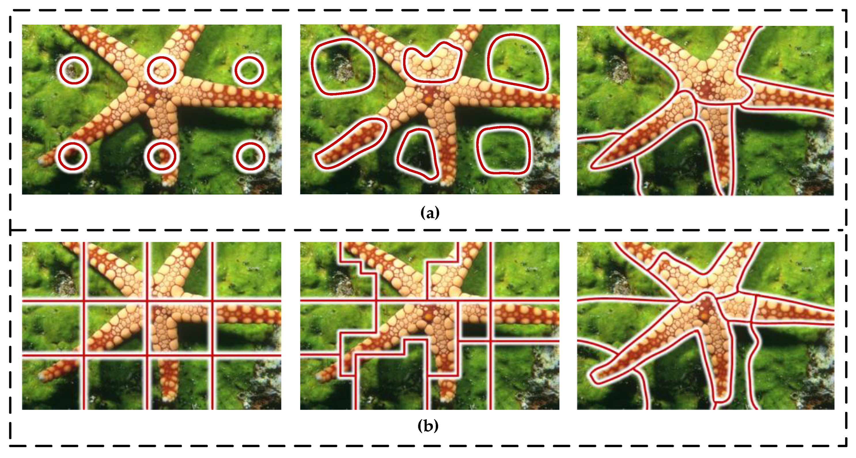
2.1. Simple Non-Iterative Clustering

Simple Linear Iterative Clustering (SLIC) [45] was proposed in 2010, which can overcome the shortcomings of traditional superpixel segmentation algorithms. The algorithm has excellent robustness and significant improvement in regard to segmentation accuracy. After that, advanced superpixels emerge one after another.

Some of these algorithms tend to pursue high boundary fit, such as Linear Spectral Clustering (LSC) [46] and Entropy-Rate Superpixels (ERS) [38]. Some focus on high efficiency, such as Iterative Boundaries Implicit Identification (IBIS) [42]. By selecting the superpixel on the boundary to move, the superpixel is continuously refined, so as to update the superpixel. Rooted Spanning Superpixels (RSS) [47] have the advantage in computing time, using the concept of minimum spanning trees to guide pixels through path-cost functions. The superpixel growth rate of this algorithm is very fast. Compromising the above two situations, quite a few researchers prefer to seek a balanced performance of speed and precision. They believe that SLIC has a good framework foundation, so a class of SLIC-like superpixel algorithms led by SLIC appears. The most representative one is the Simple Non-Iterative Clustering (SNIC) [39] algorithm developed by the creator of SLIC, which utilized a priority queue to design a non-iterative clustering framework, replacing SLIC’s K-means clustering. By changing the clustering algorithm that needs multiple iterations into a non-iterative clustering algorithm, the SNIC algorithm inherits the advantages of the SLIC algorithm and reduces the time complexity and computing memory consumption.

The problem of segmentation boundary fitting caused by the multi-scale granularity of HSIs and the computational cost result of the large data volume of HSIs are considered. We are committed to studying a superpixel algorithm for high-dimensional RS images, which takes into account boundary fitting and computational cost to some extent. It is worth mentioning that this paper will be based on SNIC in order to lay a good foundation for subsequent work. SNIC is divided into three parts and described below. The segmentation demonstration effect is shown in Figure 1a.

(1) 

Initialization stage (seed initialization based on grid sampling). In the initial phase, SNIC follows the grid initialization strategy of SLIC. Equidistant sampling in horizontal and vertical directions is carried out with a fixed step size on two-dimensional images. We take the sampling point as the initial clustering center and use it as the starting point to complete the generation and updating of superpixels.

(2) 

Correlation Measurement (color space five-dimensional joint metric). It is assumed that the two-dimensional coordinate of pixel $I_i$ of image $I$ in position space is $P\left(I_i\right)=\left[x\left(I_i\right),y\left(I_i\right)\right]$ and the three-channel color feature in CIELAB color space is $C\left(I_i\right)=\left[l\left(I_i\right),a\left(I_i\right),b\left(I_i\right)\right]$, respectively. Based on the color space joint feature, $F(I_i)=[C(I_i),P\left(I_i\right)]=\left[l(I_i),a(I_i),b(I_i),x\left(I_i\right),y\left(I_i\right)\right]$ is used for five-dimensional characterization. Accordingly, the correlation measurement between the cluster center $I_m$ and the neighborhood $I_n$ is derived from the weighted Euclidean distance of the color difference and the location difference:

$$D\left(I_m,I_n\right)=D_c(I_m,I_n)+\omega \cdot D_p(I_m,I_n)$$

(1)

where $\omega ={\displaystyle \frac{m}{S}}$, $m$ is a variable that we introduced to control the compactness of superpixels and the value range is $\left[1,20\right]$. For all the results in this article, we chose $m=10$. This experience value is derived from SNIC [39]. $S$ is the side length of the superpixel cluster. $S=\sqrt{N/K}$. $N$ is the total number of image pixels, and $K$ is the number of superpixels preset by the user.

$$D_c\left(I_m,I_n\right)={\Vert C\left(I_m\right)-C\left(I_n\right)\Vert }_2=\sqrt{\left({\left(l\left(I_m\right)-l\left(I_n\right)\right)}^2+{\left(a\left(I_m\right)-a\left(I_n\right)\right)}^2+{\left(b\left(I_m\right)-b\left(I_n\right)\right)}^2\right)}$$

(2)

$$D_p\left(I_m,I_n\right)={\Vert P\left(I_m\right)-P\left(I_n\right)\Vert }_2=\sqrt{\left({\left(x\left(I_m\right)-x\left(I_n\right)\right)}^2+{\left(y\left(I_m\right)-y\left(I_n\right)\right)}^2\right)}$$

(3)

Due to the data distribution of color space and location space being different, the value of $\omega$ reflects the importance of color and spatial location features to the similarity measurement. The different values of $\omega$ represent the variations in the characteristic tendency of superpixel boundary fit and visual comfort.

(3) 

Label allocation (allocation strategy based on online mean update). The iterative k-means algorithm is replaced by an online averaging updating system. The method of region growth is used to substitute the local candidate region traversal mode, which limits the search scope. Thus, more efficient global clustering can be achieved. In essence, this region growing is a greedy algorithm implemented using a priority queue. It converges all superpixel clusters globally into local aggregation of each cluster during the sequential generation of superpixels.

2.2. Robust Local Manifold Representation

Robust Local Manifold Representation (RLMR) [44] is an excellent hyperspectral dimension reduction method which inherits the advantages of LLE [20] and LTSA [22] in reasonably linear representation in local manifold space and can robustly solve the non-uniformity caused by data distribution. It improves the performance of classification and recognition. The RLMR comprises mainly four steps. The first two steps correspond to hierarchical neighbor selection (HNS), the third is the computation of affinity weights, and the last is the calculation of embedding.

Step 1. Joint Normalization (JN) is an effective preprocessing method for analyzing HSI. It aims to eliminate the effects of scale differences and ensure that the data are relatively uniform. This step generally begins with global data normalization (GDN) followed by local data normalization (LDN), which is a process that ranges from coarse to fine.

Step 2. Refined Neighbor Selection (RNS) mitigates the multicollinearity between spectral data to avoid affecting the subsequent model structure.

Step 3. Computation of Affinity Weights with spatial contextual information. This method adopts a robust optimization method, which has good robustness to outliers and noise.

Step 4. Low-dimensional Feature Representation is obtained by a local manifold structure in low-dimensional space.

3. Methods

In this section, we detail the hyperspectral image classification via superpixels and manifold learning, which is denoted as SMALE. Although many methods with good performance are pixel-by-pixel processing, for HSIs, pixel-by-pixel processing will bring a high probability of failure or difficult to deploy in the practical project. This is due to the large amount of HSI data, as well as information redundancy and clutter, resulting in inaccurate clustering results. SMALE maps spatial information into a dimensionality reduction framework in two key steps. This method can quickly focus on the region of interest quickly and reduce the calculation cost. First, SMALE uses SEED to obtain the HSI superpixel segmentation label with excellent performance, as described in Section 3.1. Secondly, Section 3.2 will elaborate on replacing the processing primitives of classification tasks with homogeneous superpixel blocks, mapping the original data through manifold learning into a lower-dimensional space to achieve nonlinear dimensionality reduction.

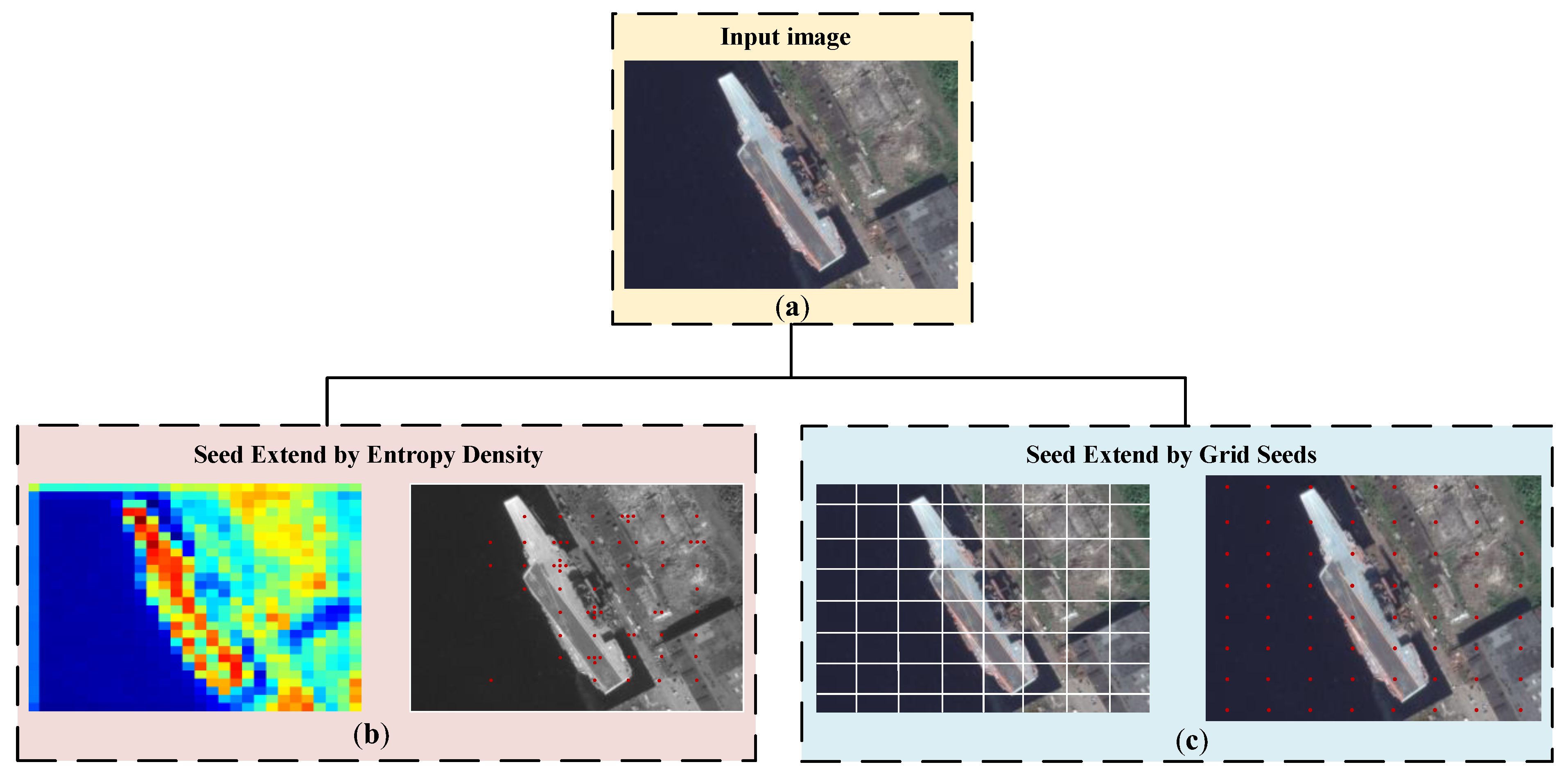
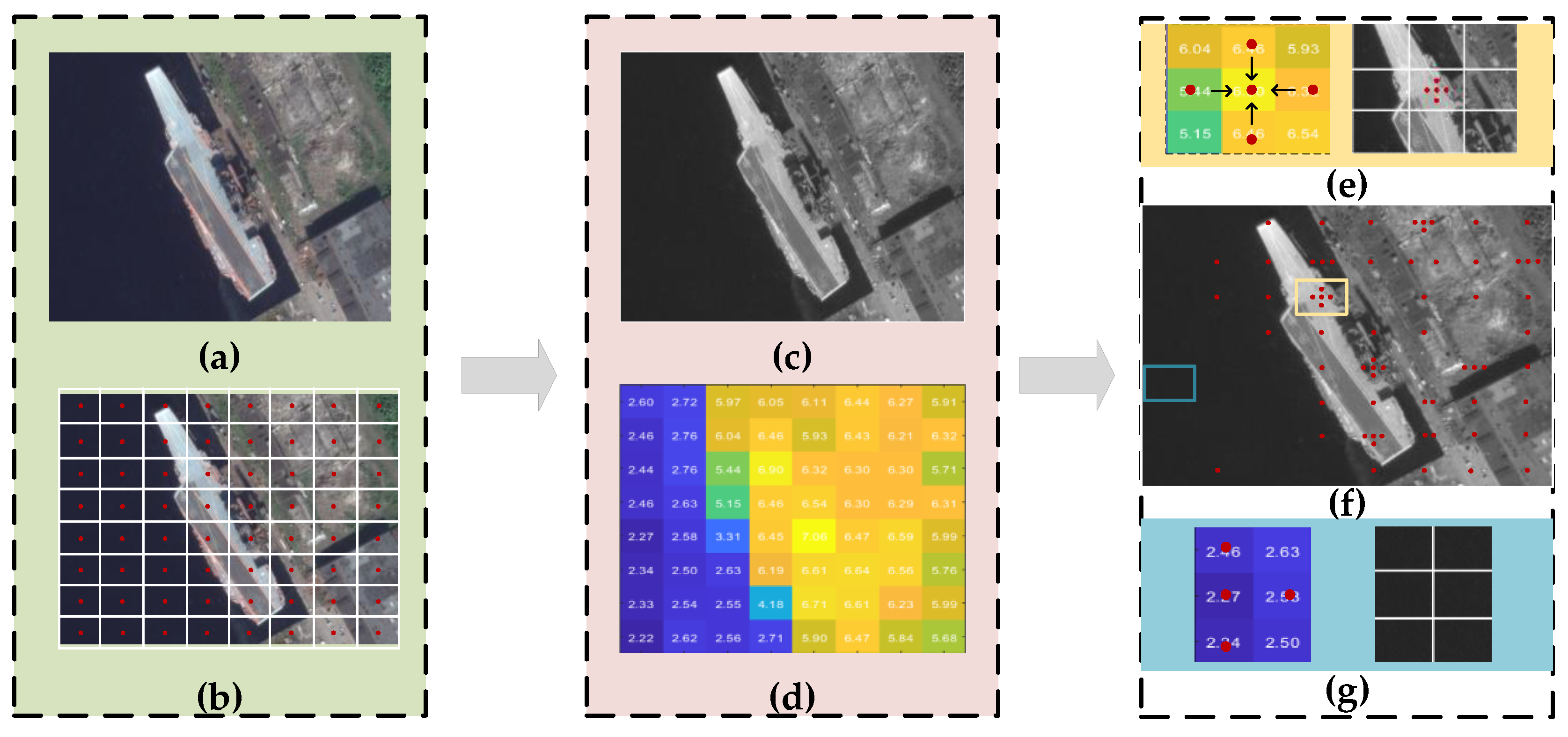
3.1. Seed Extend by Entropy Density (SEED)

In superpixel algorithms, the selection of seed points is crucial. There are methods based on uniform grids and gradient-based approaches. The grid-based method places seed points uniformly or according to a regular pattern on the image, which is used to label different regions or objects. The advantages of a grid-based seed point method include simplicity of implementation and ease of parallel processing, as shown in Figure 2b. Figure 2c uses gradient information from the image (such as Sobel or Prewitt operators) to identify pixels with high gradient magnitudes as seed points. This approach effectively captures edges and prominent transition areas in the image, making it suitable for applications that emphasize shapes and boundaries.

However, for images with uneven complexity, the grid-based seed point method does not consider intrinsic image features such as texture, color, and gradient information. This omission can lead to subsequent visual tasks lacking sufficient accuracy or adaptability. It is worth noting that gradient information effectively captures edges and transition areas in the image, but it may perform poorly in image regions with subtle gradient changes or high noise levels.

The paper improves image segmentation quality using the SEED, approached from an information-theoretic perspective. SEED can select the seed points adaptively according to the local characteristics of the image to better reflect the real structure of the image. The schematic diagram of the proposed method is shown in Figure 3 below. Figure 3b shows the distribution diagram of image content based on entropy density. According to the diagram, the seed distribution is guided, and it can be seen that simple and complex areas of the image can be easily distinguished by entropy density. Figure 3c shows the seed distribution method based on a uniform grid. The seed distribution is evenly scattered on the image without distinguishing the content.

Specifically, SEED first converts the image to grayscale, then calculates the global information entropy of the image $H_g\left(X\right)$ and the entropy of each sub-region $H_l\left(X\right)$, as shown below:

$$H_g\left(X\right)=-{\displaystyle \sum _{i=1}^{n}p\left(x_i\right)}\log p\left(x_i\right)$$

(4)

$$H_l\left(X\right)=-{\displaystyle \sum _{j=1}^{k}p\left(x_j\right)}\log p\left(x_j\right)$$

(5)

where $p\left(x_i\right)$ represents the proportion of pixels in the image with a grayscale value of $x_i$. $n$ is the total number of pixels in the image. $p\left(x_j\right)$ represents the proportion of pixels in the pixel block with a grayscale value of $x_j$. $k$ is the number of pixels in the current local pixel block.

The complexity of the current superpixel block is assessed by considering the entropy distribution of its surrounding pixels. Seed pixels are chosen based on their relatively higher local entropy. The redistribution process involves adjusting the positions of the original seed pixels to better correspond with variations in entropy across the image. This approach allows for further optimization of segmentation results while maintaining the original segmentation accuracy, which is particularly effective when dealing with images containing complex textures or transition regions. An advantage of this method lies in its adaptive adjustment of seed pixel positions, thereby enhancing both the accuracy and stability of image segmentation. A schematic diagram illustrating this process is depicted in Figure 4.

The strategy involves seed redistribution in the image. Specifically, after seeds are initially selected from pixels with a high local entropy, refined seed selection occurs based on the global entropy $H_g\left(X\right)$ and the average entropy $H_a\left(X\right)$ of sub-regions.

$$H_a\left(X\right)={\displaystyle \frac{1}{n}}{\displaystyle \sum _{i=1}^n{H}_g\left(X_i\right)}$$

(6)

• $H_l\left(X_j\right)<H_g\left(X\right)$ or $H_a\left(X\right)$, if the current area has more than one seed point, retain only one seed point. If there is a seed point in the current area, remove all;
• $H_a\left(X\right)\le H_l\left(X_j\right)\le H_g\left(X\right)$, maintain the status quo;
• $H_l\left(X_j\right)>H_g\left(X\right)$ or $H_a\left(X\right)$, If there are no seed points in the current region, add a seed point.

The pseudocode summary of SEED is presented in Algorithm 1.

Algorithm 1: SEED superpixel segmentation framework

Input: the RGB image $I$, the expected number $K$

Output: coordinates of seeds

1/*Initialization*/

2 divided the whole image into grids.

$3\mathrm{calculate}\mathrm{the}\mathrm{global}\mathrm{entropy}{H}_g\left(X\right)$ of the image $I$ by Equation (3).

4 for each cluster region $n$ do

$5\mathrm{calculate}\mathrm{the}\mathrm{entropy}{H}_l\left(X\right)$ of each sub-region by Equation (4).

6 end for

$7\mathrm{calculate}\mathrm{he}\mathrm{average}\mathrm{entropy}{H}_a\left(X\right)$ of all $n$

8         for each cluster region $n$ do

$9\mathbf{if}{H}_l\left(X_j\right)<H_g\left(X\right)$$\mathrm{or}{H}_a\left(X\right)$ then 10                 retain only one seed point. (if the current area has more than one seed point); otherwise remove all.

$11\mathbf{else}\mathbf{if}{H}_a\left(X\right)\le H_l\left(X_j\right)\le H_g\left(X\right)$ then

12                  maintain the status quo.

$13\mathbf{else}{H}_l\left(X_j\right)>H_g\left(X\right)$$\mathrm{or}{H}_a\left(X\right)$

14                  add a seed point. (if there are no seed points in the current region).

15         end if

16        end for

17        return coordinates of seeds

3.2. Space–Spectrum Model

HSI records continuous spectral information for each pixel, typically spanning tens to hundreds of spectral bands. It is stored as a multi-dimensional array, often conceptualized as a 3-D cube represented by $M\times N\times D$, where $M$ and $N$ denote the image’s height and width and $D$ represents the number of spectral bands. Superpixel segmentation usually requires a RGB image with input $m\times n\times 3$. When processing hyperspectral data, a SEED algorithm is not directly applicable, because $D\gg 3$ in HIS.

First, we need to project the hyperspectral data into the plane space for SEED segmentation. After the completion of the superpixel segmentation, the result will be mapped back to the space of the original hyperspectral data. In this process, PCA is used for processing. PCA is able to find a new set of linearly independent variables in the original data with the largest square difference. Specifically, if the data $X\in {ℝ}^{M\times N\times D}$ has $P\left(P=M\times N\right)$ samples and $D$ bands, a matrix $X$ of size $P\times D$ can be formed:

$$X=\left[\begin{array}{cccc}{x}_{11}& x_{12}& \cdots & x_{1D}\\ x_{21}& x_{22}& \cdots & x_{2D}\\ ⋮& ⋮& \ddots & ⋮\\ x_{P1}& x_{P1}& \cdots & x_{PD}\end{array}\right]=\left(x_1,x_2,\cdots ,x_D\right)$$

(7)

The linearly independent variable $z_1,z_2,\cdots ,z_d\left(d\le D\right)$ with the maximum variance, and they satisfy:

$$\{\begin{array}{c}{z}_1={\mathrm{l}}_{11}{x}_1+{\mathrm{l}}_{12}{x}_2+\cdots +{\mathrm{l}}_{1D}{x}_D\\ z_2={\mathrm{l}}_{21}{x}_1+{\mathrm{l}}_{22}{x}_2+\cdots +{\mathrm{l}}_{2D}{x}_D\\ \cdots \\ z_d={\mathrm{l}}_{d1}{x}_1+{\mathrm{l}}_{d2}{x}_2+\cdots +{\mathrm{l}}_{dD}{x}_D\end{array}$$

(8)

The principles for determining coefficients ${\mathrm{l}}_{ij}$ are as follows:

• $z_1$ is unrelated to $z_2$ ($i\ne j;i,j=1,2,\dots ,d$);
• $z_1$ is the linear combination with the maximum variance among $x_1,x_2,\cdots ,x_D$;
• $z_2$ is the linear combination with the maximum variance among all linear combinations of $x_1,x_2,\cdots ,x_D$ that are uncorrelated with $z_1$;
• Continuing in this manner, $z_d$ is the linear combination with the maximum variance among all linear combinations of $x_1,x_2,\cdots ,x_D$ that are uncorrelated with $z_1,z_2,\cdots ,z_{d-1}$;
• The new variables $z_1,z_2,\cdots ,z_d$ are, respectively, referred to as the first, second, …, $d\mathrm{th}$ principal components of the original variables $x_1,x_2,\cdots ,x_D$.

Following the above operations, we use superpixel blocks instead of traditional pixels. The superpixel block is treated as the new basic processing unit, and the hyperspectral data are denoted as $X_{\mathrm{sp}}\in {ℝ}^{K\times D}$, while $K$ is the number of superpixels. These blocks represent contiguous regions in the image, where each superpixel block can be viewed as a small block that merges similar spectral and spatial information. These features better capture the spatial and spectral information integrity in HSIs.

Inspired by LLE [20], we capture the underlying local manifold structure of hyperspectral blocks processed through superpixels and preserve it in a low-dimensional space. Without loss of generality, the spatial–spectral dimensionality reduction model proposed in this paper mainly includes the steps shown in Figure 5. As explained in Section 2.2, the dimensionality reduction framework based on manifold is generally divided into the following three steps: (1) selection of neighbor points, as shown in Figure 5a; (2) weight calculation, as shown in Figure 5d; (3) embedded calculation, as shown in Figure 5e. On this basis, SMALE adds the SEED superpixel segmentation part, as shown in Figure 5c. The spatial information provided by SEED and the spectral information of the HSI make the dimensionality reduction based on the manifold more robust.

Let $W\in {ℝ}^{K\times K}$ denote a sparse affinity matrix, where each entry $\left(i,j\right)$ represents the affinity weight between the $i\mathrm{th}$ and $j\mathrm{th}$ superpixel blocks. The spectral data after dimensionality reduction is denoted as $Y=[y_1,y_2,\dots ,y_K]\in {ℝ}^{K\times d}$, where $d\gg D$. The calculation of embedding coordinates is generally formulated as follows:

$$\widehat{Y}=\arg \underset{Y}{\min }\left\{{\displaystyle \sum _{i=1}^K{\displaystyle \sum _{j\in {\varphi }_i}{\Vert y_i-y_j\Vert }_2^2{W}_{ij}}}\right\},\mathrm{s}.\mathrm{t}.YB{Y}^T=I$$

(9)

where ${\varphi }_{\mathrm{i}}$ is a set of neighbors of the $i\mathrm{th}$ superpixel block. $B$ is a constant matrix defined according to different manifold learning methods.

This paper adopts the optimization framework of local linear embedding. It considers the reconstruction symmetry of each data point and its neighborhood points to design its method.

Accordingly, we apply it between the superpixel blocks, then calculate the reconstruction coefficient between the superpixel blocks and embed the calculation. The reconstruction coefficient is obtained by minimization, denoted as $\widehat{A}\in {ℝ}^{K\times K}$.

$$\widehat{A}=\arg \underset{A}{\min }\left\{{{\displaystyle \sum _{i=1}^K\Vert x_i-{\displaystyle \sum _{j\in {\varphi }_i}{A}_{ij}{x}_{ij}}\Vert }}_2^2\right\},\mathrm{s}.\mathrm{t}.{\displaystyle \sum _{j\in {\varphi }_i}{A}_{ij}}=1$$

(10)

The formula for calculating its low-dimensional coordinates is as follows:

$$\begin{array}{l}\widehat{Y}=\arg \underset{Y}{\min }\left\{{{\displaystyle \sum _{i=1}^K\Vert y_i-{\displaystyle \sum _{j\in {\varphi }_i}{A}_{ij}{y}_j}\Vert }}_2^2\right\}\\ \mathrm{s}.\mathrm{t}.{\displaystyle \frac{1}{K}}{\displaystyle \sum _{i=1}^K{y}_i{y_i}^{\mathrm{T}}}=I, {\displaystyle \sum _{i=1}^K{y}_i=0}.\end{array}$$

(11)

where it should be noted that $A_{ij}$ represents the reconstruction weight between $x_i$ and $x_j$; if $j\mathrm{th}$ data are not in the $i\mathrm{th}$ data’s neighborhood, then $A_{ij}=0$.

Combining Equations (8) and (10), we obtain the following:

$$W_{ij}=A_{ij}+A_{ji}-A_{ij}{A}_{ji}$$

(12)

The optimized LLE model can not only obtain the local manifold structure but also capture the spatial characteristics of the data after superpixel processing. In the stage of neighborhood selection, the constraint range can be more accurate and the reconstruction error of local manifold structures in low dimensional space and structure reconstruction in high-dimensional space can be reduced.

4. Experiment and Discussion

This section aims to demonstrate the effectiveness of the SEED algorithm specifically designed for HSIs and its rational application within the Locally Linear Embedding (LLE) framework. While there are no readily available hyperspectral datasets tailored specifically for validating superpixel segmentation algorithms, the validity of the SEED algorithm can be verified through appropriate preprocessing and evaluation methods. Firstly, the superpixel dataset and hyperspectral dataset used in this paper are introduced. Secondly, SEED is comprehensively evaluated from both qualitative and quantitative perspectives compared against classical and state-of-the-art superpixel algorithms. Finally, an ablation experiment is designed to prove the excellent performance of the SMALE dimensionality reduction framework in classification tasks.

4.1. Experiment Setup

One superpixel segmentation dataset and two hyperspectral datasets are used in this experiment, which are described in detail in Section 4.1.1 and Section 4.1.2, respectively. All methods are executed on an Intel Core i7 4.2 GHz with 16 GB RAM without any parallelization or GPU processing.

4.1.1. Superpixel Segmentation Dataset

A Berkeley Segmentation Dataset (BSDS) [49] is a classic image segmentation dataset created by the Computer Vision Lab at the University of California, Berkeley. The BSDS contains hundreds of real-world images of natural scenes that cover a variety of complex visual situations and scenes. Each image is manually marked by an expert or highly trained marker to mark the boundaries and divisions of the individual objects. Therefore, it is considered to be a high-quality and reliable segmentation result.

4.1.2. Hyperspectral Datasets

The Indian Pines dataset [50] is a classic HSI classification dataset that is often used to test and evaluate the performance of HSI-processing and analysis algorithms. The Indian Pines dataset consists of a 145 × 145 pixels HSI covering 16 categories. Each pixel has 220 bands of information on the spectrum, which makes the dataset ideal for research and development of image processing algorithms involving spectral information.

The Salinas A dataset [32] is a widely used standard dataset for hyperspectral image analysis, sourced from an aerial RS mission over Salinas County, California. It includes HSIs with multiple bands, covering a range from visible to near-infrared wavelengths, and features high-spatial and-spectral resolutions. The image resolution is 83 × 86 pixels, with each pixel containing over 200 spectral bands. The primary uses of the Salinas A dataset include land cover classification, target detection, and anomaly detection. It provides researchers with a rich hyperspectral data source for algorithm development and performance evaluation. Due to its detailed spectral characteristics and comprehensive land cover information, the Salinas A dataset holds significant importance in regard to HSI processing and RS technology research.

4.2. Results of BSDS Data

In this section, the performance of SEED is qualitative and quantitative to verify its advancement. To demonstrate objectivity, we randomly selected 200 images in the data as a test set. We will list some of the representative segmentation effects and local details. In addition, several common evaluation indexes [51] are provided to quantify the accuracy of the image boundary and the segmentation results, such as Boundary Recall (BR), Achievable Segmentation Accuracy (ASA), Under-segmentation Error (UE), and Compactness (CO).

4.2.1. Visual Assessment

The qualitative analysis of the superpixel algorithm is demonstrated by a visual segmentation effect. Figure 6 shows seven superpixel algorithms, including SEED. SNIC is recognized as a classical superpixel generation algorithm. The ERS algorithm is the choice for most HSIs that use superpixels. Through visual analysis, we can intuitively see whether the segmentation result fits the target edge and whether there is over-segmentation. From the overall segmentation effect, the result of WSGL and ERS are messy and have poor anti-texture abilities compared with other algorithms, but these two algorithms perform well in capturing details. It can be seen that the pursuit of precision is to sacrifice the regularity of the shape of the superpixel block. It is worth mentioning that SEED seeks exactly this balance. As the partial zoom shows, the superpixels generated by SEED are uniform, compact, and, most importantly, excellent at fitting boundaries. The appearance of MBS is very neat, and the segmentation accuracy is also high, but its accuracy is not high in areas of similar colors, and it is also easily affected by similar colors. SEED also successfully overcomes this problem. Overall, SEED’s competitiveness is clear.

4.2.2. Metric Evaluation

In this section, SEED and other state-of-the-art algorithms will be comprehensively evaluated based on the four indexes commonly used to verify superpixel algorithms.

• Boundary Recall (BR): BR is an important index to measure the ability of the algorithm to detect the real target boundary. Specifically, BR stands for the ability to correctly locate and cover the boundaries of real targets. The value of BR ranges from 0 to 1. The higher the value, the greater the proportion of the detected bounding box covering the real target boundary, i.e., the better the algorithm performance. Its calculation formula is as follows:

  $$\mathrm{BR}={\displaystyle \frac{{\displaystyle {\sum }_{i\in {\Phi }_B}\prod \left({\min }_{j\in {\Omega }_B}\Vert P\left(I_i\right)-P\left(I_j\right)\Vert <r\right)}}{{\Phi }_B}}$$

  (13)

  where ${\Phi }_B$ and ${\Omega }_B$ represent the boundary pixels in the set. $\prod ( )$ represents the logic value of 0 or 1. $P\left(I_i\right)=\left[x\left(I_i\right),y\left(I_i\right)\right]$ and $r$ is set to two pixels.
• Under-segmentation Error (UE): UE evaluates the difference between the segmentation boundary generated by the algorithm and the real segmentation boundary. It focuses on areas or parts of the segmentation result that do not segment the target correctly. Specifically, it can be defined by the following formula:

  $$\mathrm{UE}={\displaystyle \frac{{\displaystyle \sum _{m=1}^M\left({\displaystyle {\sum }_{{\Omega }_k|{\Omega }_k\cap {\Phi }_m\ne \varphi }\left|{\Omega }_k\right|}\right)}-N}{N}}$$

  (14)

  where $N$ is the number of pixels in the image. $\Omega ={\left\{{\Omega }_k\right\}}_{k=1}^K$ and $\Phi ={\left\{{\Phi }_m\right\}}_{m=1}^M$ represent the calculated superpixels and the ground truth of the same image ${\left\{I_i\right\}}_{i=1}^N$, respectively.
• Achievable Segmentation Accuracy (ASA): ASA is an index used to evaluate the performance of segmentation algorithms in image segmentation tasks. It is designed to measure the highest level of segmentation accuracy that an algorithm can achieve. It is usually deduced or calculated by some theoretical analysis or idealized algorithm.

  $$\mathrm{ASA}={\displaystyle \frac{{\displaystyle \sum _{k=1}^K\arg \max \left|{\Omega }_k\cap {\Phi }_m\right|}}{{\displaystyle \sum _{m=1}^M\left|{\Phi }_m\right|}}}$$

  (15)
• Compactness (CO): CO is an index used to measure the compactness of segmentation results in an image segmentation evaluation. It is mainly concerned with the shape compactness of the segmented area or object.

  $$\mathrm{CO}={\displaystyle \sum _{i=1}^K\frac{4\pi {\xi }_{S{P}_i}\ast \left|S{P}_i\right|}{{\psi }_{S{P}_i}^2\ast \left|I\right|}}$$

  (16)

  where ${\xi }_{S{P}_i}$ and ${\psi }_{S{P}_i}$ are expressed as the area and perimeter of the $i\mathrm{th}$ superpixel, respectively.

Figure 7 shows the test results of the above metrics on all algorithms. The red curve is the performance of the algorithm SEED proposed in this paper. As illustrated in Figure 7, SEED performs well in terms of the highest level of segmentation accuracy that can be achieved. At the same time, the number of pixels wrongly divided in the segmentation result is the fewest. Figure 7e is the compactness index corresponding to the qualitative analysis in Figure 7. The MBS visual effect is both compact and regular, and its CO indicator performs best. A larger CO value indicates that the shape of the divided area is not too scattered or complex.

4.3. Results of Indian Pines Dataset

In this section, we compare the proposed space–spectrum model-SMALE with traditional and state-of-the-art methods on the India Pines dataset [50]. It is worth noting that, in order to prove that SEED plays a catalytic role, we will replace the superpixel part of SMALE with MBS and ERS, designed as a cross test for benchmarking. Due to the large number of categories in the India Pines dataset, the dataset is considered challenging. As shown in Figure 8, SMALE demonstrated competitive precision in its ability to identify various crops. Classification accuracy is almost perfect in the Woods and Hay-windrowed regions. RLMR can be comparable, but its overall classification accuracy needs to be improved.

In this paper, the quantitative analysis is reflected by OA, AA, and Kappa [54]. The specific quantitative indicators are shown in

Table 1. Classification result of the proposed method and ten comparison algorithms on an Indian Pines dataset.

Evaluation Index		Algorithm
	PCA	KPCA	LLE	LTSA	SuperPCA	RLMR	S2DL	D-VIC	ERS-LLE	MBS-LLE	SMALE
OA (%)	64.35	67.03	68.23	72.06	89.26	80.65	73.25	52.35	78.41	80.78	90.74
AA (%)	73.42	76.98	75.71	80.96	93.55	89.66	65.32	53.27	86.77	90.65	95.28
Kappa	0.3315	0.3996	0.4365	0.4735	0.5008	0.5211	0.5920	0.4020	0.5332	0.5572	0.5691

.

• Overall Accuracy (OA): OA is a measure of the proportion of the classifier’s predictions that are correct across the entire dataset. It is the most simple and intuitive classification performance evaluation indicator, and it is calculated as follows:

  $$\mathrm{OA}={\displaystyle \frac{\left(TP+TN\right)}{\left(TP+FN+FP+TN\right)}}$$

  (17)
• Average Accuracy (AA): AA refers to the average accuracy of each class. In a multi-class classification problem, different classes may have different sample sizes and levels of importance. AA provides a more detailed assessment by calculating the classification accuracy of each category and averaging it.

  $$\mathrm{AA}={\displaystyle \frac{1}{N}}{\displaystyle {\sum }_{i=1}^r{x}_{ii}}$$

  (18)

  where $N$ is the total number of pixels. $x_{ii}$ is the value on the diagonal of its confusion matrix.
• Kappa is a measure of consistency between the classifier’s predictions and ground truth. It takes into account the adjustment of the correctness of model predictions and the factors of random predictions, so it is particularly useful for working with categorically unbalanced datasets.

  $$\mathrm{Kappa}={\displaystyle \frac{N{\displaystyle {\sum }_{i=1}^{\mathrm{r}}{x}_{ii}-}{\displaystyle {\sum }_{i=1}^{\mathrm{r}}\left(x_{i+}\times x_{+i}\right)}}{N^2-{\displaystyle {\sum }_{i=1}^{\mathrm{r}}\left(x_{i+}\times x_{+i}\right)}}}$$

  (19)

  where $x_{i+}$ is the number of actual reference pixels in each category and $x_{+i}$ is the total number of classified pixels in the class.

It is worth mentioning that this paper explores the influence of superpixels on the dimensionality reduction framework. In addition to the above experiments, we conducted more detailed experiments on the design of the superpixel module, conducted multi-scale experiments with different displays involving the numbers in the superpixels set, and conducted statistics for each category of the India Pines dataset. The data analysis is shown in

Table 2. Performance of the proposed SMALE model on the Indian Pines dataset, with the expected number of superpixels ranging from 50 to 500.

Class Names	Expected Superpixel Number
	50	100	150	200	250	300	350	400	450	500
Corn-notill	68.57	72.89	78.22	93.65	87.36	85.64	80.37	70.36	66.75	62.37
Corn-mintill	83.88	90.09	92.51	96.87	95.66	94.28	93.71	89.65	82.54	80.32
Corn	92.65	95.88	96.41	99.21	98.55	97.62	97.21	94.56	90.98	90.23
Grass-pasture	92.36	93.55	93.96	96.88	95.12	94.87	94.45	92.89	91.63	90.72
Grass-trees	82.63	89.68	90.63	96.87	95.21	94.66	92.45	85.52	80.87	78.65
Hay-windrowed	97.32	97.32	97.32	100	99.62	99.23	98.76	97.32	96.78	95.62
Soybean-notill	85.74	90.43	91.25	95.22	92.22	91.25	91.25	89.66	80.65	70.85
Soybean-mintill	90.25	91.65	94.55	97.10	96.10	95.43	95.22	90.36	89.67	88.34
Soybean-clean	80.66	85.98	86.87	94.98	92.55	90.02	89.21	81.30	79.65	78.33
Wheat	97.65	99.56	99.56	98.56	99.20	99.21	99.56	98.13	96.26	95.13
Woods	80.48	90.31	91.47	98.77	98.44	98.22	95.67	81.61	78.15	70.26
Bldg-Gra-Tr-Driv	96.36	98.06	98.00	100	99.25	98.65	98.43	97.28	94.58	90.88
Stone-Steel-Towers	99.02	100	100	98.97	98.97	99.33	99.52	100	98.55	97.65
Alfalfa	96.52	97.22	97.86	100	100	99.65	98.10	96.66	95.32	94.99
Grass-pasture-mowed	96.11	97.89	97.89	98.89	97.89	97.89	97.89	97.85	95.65	94.98
Oats	98.65	99.01	99.77	100	100	100	100	98.78	96.00	95.02
OA (%)	87.52	92.15	93.00	95.89	94.62	94.26	93.45	90.33	85.66	82.26
AA (%)	89.93	93.09	94.14	97.87	96.64	95.99	95.11	91.37	88.38	85.89

.

Based on the above experiments, we can conclude that the optimal number of superpixels in Indian Pines is 200. The trend in the table data shows that the classification accuracy increases first and then decreases with the increase in the number of superpixels. This is because the size of the dataset is 145 × 145 × 200, and the two-dimensional size itself is not large. Setting too many superpixels will lead to over-segmentation, and the classification accuracy cannot be reached.

In order to more obviously prove that the appropriate superpixel algorithm can improve the classification accuracy, we deliberately selected all the classification algorithms based on the superpixels for further analysis (ERS-LLE, MBS-LLE, SuperPCA, S²DL, SMALE). As shown in Figure 9, there is no doubt that the best performance is SMALE, and the OA of RLMR also shows considerable advantages. Because both ERS-DR and SuperPCA employ ERS for superpixel preprocessing, their OA trends are similar. In general, when the number of superpixels is 200, the classification accuracy of each algorithm reaches its peak, which confirms the conclusion drawn from Table 2.

4.4. Results of Salinas a Dataset

To demonstrate the versatility of SMALE, we continue our experiments on the hyperspectral dataset Salinas A, as shown in Figure 10. SMALE achieved near-perfect classification accuracy on the Salinas A, outperforming its competitors in performance despite the unsupervised setup of our algorithm. The classification framework firstly applies superpixel technology to segment HSI and decompose them into regions with high spectral similarities. This step effectively reduces the computational complexity and improves the robustness of classification. Then, we use the manifold learning method to reduce the dimensionality of the superpixels and extract the structural features of the low-dimensional manifold to facilitate the subsequent classification task. Compared with Indian Pines, the performance of the ten algorithms on Salinas A has improved, but PCA still cannot fully explore the potential structure of the data, resulting in a limited classification performance. KPCA extends PCA to capture the nonlinear structure of the data through the kernel function, but, in the course of the experiment, we found that the performance of KPCA is highly dependent on the choice of kernel function. If the kernel function selected cannot effectively capture the nonlinear structure of the data, it may lead to a poor dimensionality reduction. In terms of computational complexity, when processing large-scale data, computational complexity and memory consumption may be very high, resulting in low algorithm efficiency. SuperPCA combines superpixel segmentation and traditional PCA to reduce dimensionality through superpixel blocks. This method improves the structured processing and dimensionality reduction in data. The S²DL is second only to SMALE, with an overall accuracy of 99.69%, which is also near perfect. RLMR further optimizes manifold learning by regularization technology, which makes the dimensionality reduction process more stable and efficient. The classification effect of RLMR on the Salinas A dataset is usually better than that of traditional manifold learning methods, which can provide high classification accuracy in complex environments.

In summary, the dimensionality reduction classification framework based on superpixels and manifold learning performs better with the Salinas A dataset than the simple dimensionality reduction method. By capturing the nonlinear and complex structure of the data, the classification effect is significantly improved.

Table 3. Classification result of the proposed method and ten comparison algorithms on the Salinas A dataset.

Evaluation Index		Algorithm
	PCA	KPCA	LLE	LTSA	SuperPCA	RLMR	S2DL	D-VIC	ERS-LLE	MBS-LLE	SMALE
OA (%)	86.54	88.62	89.23	92.06	97.26	93.56	99.10	96.51	98.23	98.41	99.28
AA (%)	86.98	88.98	92.71	93.96	97.55	95.25	99.69	97.20	98.87	98.65	99.74
Kappa	0.8315	0.8696	0.83415	0.8765	0.9308	0.9211	0.9840	0.9652	0.9632	0.9572	0.9915

shows the quantitative classification results of SMALE and ten comparison algorithms in the Salinas A dataset, which are also explained through OA, AA, and Kappa.

It can be analyzed from Table 3 that the performances of eleven classification frameworks, including SMALE, in the Salinas A dataset have been greatly improved. Among them, the classification accuracy of eight frameworks is above 90%, and the performance of their Kappa index is also above 0.83, among which that of SMALE is as high as 0.9915. This index mainly measures the degree of consistency between classification results and random classification, and its value range is $[-1,1]$. The higher the classification result is, the more consistent the classification result is with the actual category. The result of the classification is in good agreement with the actual category, which indicates that the model can predict the target category well.

5. Conclusions

In this paper, a superpixel generation framework called Seed Extend by Entropy Density (SEED) is proposed for practical application. In this work, we focus on designing a superpixel seed redistribution framework that can directly and effectively replace the initialization strategy of grid sampling. This algorithm can solve the problem that the region of interest is difficult to focus on due to the diversity of hyperspectral image content. By combining the five-dimensional color–space information in superpixels with the spectral information of hyperspectral data, a novel space–spectrum feature constraint model, SMALE, is constructed which can improve and optimize the classification of hyperspectral images globally and solve the problem that image processing takes too much time and is difficult to be practical. The experiment showed that SEED had excellent performance, reaching the highest ASA (0.9535%) and the lowest UE (0.0369%) while maintaining the leading level of BR and CO. At the same time, the SMALE model had a classification accuracy of 97.8700% in the Indian Pines dataset and 99.7453% on the Salinas A dataset. It has been proven that SEED has a positive effect on classification accuracy.

Future work will focus more on the application of superpixels in a variety of RS tasks, such as change detection, ground object recognition, ROI extraction, and other visual tasks. Future works should also make better use of superpixels as an efficient tool. We will look at designing superpixel algorithms with personalizations for different tasks.

References

1. Bioucas-Dias, J.M.; Plaza, A.; Camps-Valls, G.; Scheunders, P.; Nasrabadi, N.; Chanussot, J. Hyperspectral Remote Sensing Data Analysis and Future Challenges. IEEE Geosci. Remote Sens. Mag. 2013, 1, 6–36. [Google Scholar] [CrossRef]
2. He, L.; Li, J.; Liu, C.; Li, S. Recent Advances on Spectral-Spatial Hyperspectral Image Classification: An Overview and New Guidelines. IEEE Trans. Geosci. Remote Sens. 2018, 56, 1579–1597. [Google Scholar] [CrossRef]
3. Han, Z.; Zhang, H.; Li, P.; Zhang, L. Hyperspectral image clustering: Current achievements and future lines. IEEE Geosci. Remote Sens. Mag. 2021, 9, 35–67. [Google Scholar]
4. Lu, B.; Dao, P.D.; Liu, J.; He, Y.; Shang, J. Recent Advances of Hyperspectral Imaging Technology and Applications in Agriculture. Remote Sens. 2020, 12, 2659. [Google Scholar] [CrossRef]
5. Fauvel, M.; Tarabalka, Y.; Benediktsson, J.A.; Chanussot, J.; Tilton, J.C. Advances in spectral-spatial classification of hyperspectral images. Proc. IEEE. 2013, 101, 652–675. [Google Scholar] [CrossRef]
6. Zhang, L.; Zhang, L.; Du, B. Deep learning for remote sensing data: A technical tutorial on the state of the Art. IEEE Geosci. Remote Sens. Mag. 2016, 4, 22–40. [Google Scholar] [CrossRef]
7. Ma, J.; Jiang, J.; Zhou, H.; Zhao, J.; Guo, X. Guided locality pre-serving feature matching for remote sensing image registration. IEEE Trans. Geosci. Remote Sens. 2018, 56, 4435–4447. [Google Scholar] [CrossRef]
8. Ma, J.; Chen, C.; Li, C.; Huang, J. Infrared and visible image fusion via gradient transfer and total variation minimization. Inf. Fusion 2016, 31, 100–109. [Google Scholar] [CrossRef]
9. Melgani, F.; Bruzzone, L. Classification of hyperspectral remote sensing images with support vector machines. IEEE Trans. Geosci. Remote Sens. 2004, 42, 1778–1790. [Google Scholar] [CrossRef]
10. Liu, G.; Wang, L.; Liu, D.; Fei, L.; Yang, J. Hyperspectral Image Classification Based on Non-Parallel Support Vector Machine. Remote Sens. 2022, 14, 2447. [Google Scholar] [CrossRef]
11. Kang, J.; Zhang, Y.; Liu, X.; Cheng, Z. Hyperspectral Image Classification Using Spectral–Spatial Double-Branch Attention Mechanism. Remote Sens. 2024, 16, 193. [Google Scholar] [CrossRef]
12. Liu, G.; Wang, L.; Liu, D. Hyperspectral Image Classification Based on a Least Square Bias Constraint Additional Empirical Risk Minimization Nonparallel Support Vector Machine. Remote Sens. 2022, 14, 4263. [Google Scholar] [CrossRef]
13. Schölkopf, B.; Smola, A.; Müller, K.-R. Nonlinear component analysis as a kernel eigenvalue problem. Neural Comput. 1998, 10, 1299–1319. [Google Scholar] [CrossRef]
14. Prasad, S.; Bruce, L.M. Limitations of principal components analysisfor hyperspectral target recognition. IEEE Geosci. Remote Sens. Lett. 2008, 5, 625–629. [Google Scholar] [CrossRef]
15. Wang, J.; Chang, C.-I. Independent component analysis-based dimensionality reduction with applications in hyperspectral image analysis. IEEE Trans. Geosci. Remote Sens. 2006, 44, 1586–1600. [Google Scholar] [CrossRef]
16. Schölkopf, B.; Smola, A.; Müller, K.R. Kernel principal component analysis. In Artificial Neural Networks—ICANN’97; Gerstner, W., Germond, A., Hasler, M., Nicoud, J.D., Eds.; Lecture Notes in Computer Science; Springer: Berlin/Heidelberg, Germany, 1997; Volume 1327, pp. 583–588. [Google Scholar]
17. Bach, F.R.; Jordan, M.I. Kernel independent component analysis. J. Mach. Learn. Res. 2002, 3, 1–48. [Google Scholar]
18. Mika, S.; Ratsch, G.; Weston, J.; Scholkopf, B.; Mullers, K.R. Fisher discriminant analysis with kernels. In Neural Networks for Signal Processing IX: Proceedings of the 1999 IEEE Signal Processing Society Workshop (Cat. No.98TH8468); IEEE: Piscataway, NJ, USA, 1999; pp. 41–48. [Google Scholar]
19. Tenenbaum, J.B.; De Silva, V.; Langford, J.C. A global geometric framework for nonlinear dimensionality reduction. Science 2000, 290, 2319–2323. [Google Scholar] [CrossRef]
20. Roweis, S.T.; Saul, L.K. Nonlinear dimensionality reduction by locally linear embedding. Science 2000, 290, 2323–2326. [Google Scholar] [CrossRef]
21. Belkin, M.; Niyogi, P. Laplacian eigenmaps for dimensionality reduction and data representation. Neural Comput. 2003, 15, 1373–1396. [Google Scholar] [CrossRef]
22. Zhang, Z.; Zha, H. Principal manifolds and nonlinear dimension reduction via local tangent space alignment. SIAM J. Sci. Comput. 2004, 26, 313–338. [Google Scholar] [CrossRef]
23. Bachmann, C.M.; Ainsworth, T.L.; Fusina, R.A. Exploiting manifold geometry in hyperspectral imagery. IEEE Trans. Geosci. Remote Sens. 2005, 43, 441–454. [Google Scholar] [CrossRef]
24. He, J.; Zhang, L.; Wang, Q.; Li, Z. Using diffusion geometric coordinates for hyperspectral imagery representation. IEEE Trans. Geosci. Remote Sens. 2009, 6, 767–771. [Google Scholar]
25. Ma, L.; Crawford, M.M.; Tian, J.W. Local manifold learning-based k-nearest-neighbor for hyperspectral image classification. IEEE Trans. Geosci. Remote Sens. 2010, 48, 4099–4109. [Google Scholar] [CrossRef]
26. Ma, L.; Crawford, M.M.; Yang, X.; Guo, Y. Local-manifold-learning-based graph construction for semisupervised hyperspectral image classification. IEEE Trans. Geosci. Remote Sens. 2015, 53, 2832–2844. [Google Scholar] [CrossRef]
27. Huang, H.; Huo, H.; Fang, T. Hierarchical manifold learning with application to supervised classification for high-resolution remotely sensed images. IEEE Trans. Geosci. Remote Sens. 2013, 52, 1677–1692. [Google Scholar] [CrossRef]
28. Tan, Y.; Yuan, H.; Li, L. Manifold-based sparse representation for hyperspectral image classification. IEEE Trans. Geosci. Remote Sens. 2014, 52, 7606–7618. [Google Scholar]
29. Yang, H.L.; Crawford, M.M. Spectral and spatial proximity-based manifold alignment for multitemporal hyperspectral image classification. IEEE Trans. Geosci. Remote Sens. 2016, 54, 51–64. [Google Scholar] [CrossRef]
30. Ma, L.; Crawford, M.M.; Tian, J.W. Anomaly detection for hyperspectral images based on robust locally linear embedding. J. Infrared Millim. THz Waves 2010, 31, 753–763. [Google Scholar] [CrossRef]
31. Sui, C.; Li, C.; Feng, J.; Mei, X. Unsupervised Manifold-Preserving and Weakly Redundant Band Selection Method for Hyperspectral Imagery. IEEE Trans. Geosci. Remote Sens. 2020, 58, 1156–1170. [Google Scholar] [CrossRef]
32. Jiang, J.; Ma, J.; Chen, C.; Wang, Z.; Cai, Z.; Wang, L. SuperPCA: A Superpixelwise PCA Approach for Unsupervised Feature Extraction of Hyperspectral Imagery. IEEE Trans. Geosci. Remote Sens. 2018, 56, 4581–4593. [Google Scholar] [CrossRef]
33. Zhang, L.; Su, H.; Shen, J. Hyperspectral Dimensionality Reduction Based on Multiscale Superpixelwise Kernel Principal Component Analysis. Remote Sens. 2019, 11, 1219. [Google Scholar] [CrossRef]
34. Cortes, C.; Vapnik, V. Support-Vector Networks. Mach. Learn. 1995, 20, 273–297. [Google Scholar] [CrossRef]
35. Liao, N.; Guo, B.; Li, C.; Liu, H.; Zhang, C. BACA: Superpixel segmentation with boundary awareness and content adaptation. Remote Sens. 2022, 14, 4572. [Google Scholar] [CrossRef]
36. Li, C.; Guo, B.; Liao, N.; Gong, J.; He, W. CONIC: Contour Optimized Non-Iterative Clustering Superpixel Segmentation. Remote Sens. 2021, 13, 1061. [Google Scholar] [CrossRef]
37. Liao, N.; Guo, B.; He, F.; Li, W.; Li, C.; Liu, H. Spherical Superpixel Segmentation with Context Identity and Contour Intensity. Symmetry 2024, 16, 925. [Google Scholar] [CrossRef]
38. Liu, M.-Y.; Tuzel, O.; Ramalingam, S.; Chellappa, R. Entropy rate superpixel segmentation. In Proceedings of the IEEE Conference on Computer Vision and Pattern Recognition (CVPR), Colorado Springs, CO, USA, 20–25 June 2011; pp. 2097–2104. [Google Scholar]
39. Achanta, R.; Susstrunk, S. Superpixels and polygons using simple non-iterative clustering. In Proceedings of the IEEE Conference on Computer Vision and Pattern Recognition (CVPR), Honolulu, HI, USA, 21–26 July 2017; pp. 4651–4660. [Google Scholar]
40. Hu, Y.; Li, Y.; Song, R.; Rao, P.; Wang, Y. Minimum barrier superpixel segmentation. Image Vis. Comput. 2018, 70, 1–10. [Google Scholar] [CrossRef]
41. Yuan, Y.; Zhu, Z.; Yu, H.; Zhang, W. Watershed-Based Superpixels with Global and Local Boundary Marching. IEEE Trans. Image Process. 2020, 29, 7375–7388. [Google Scholar] [CrossRef]
42. Bobbia, S.; Macwan, R.; Benezeth, Y. Iterative Boundaries implicit Identification for superpixels Segmentation: A real-time approach. IEEE Access 2021, 9, 77250–77263. [Google Scholar] [CrossRef]
43. Li, C.; He, W.; Liao, N.; Gong, J.; Hou, S.; Guo, B. Superpixels with contour adherence via label expansion for image decomposition. Neural Comput. Appl. 2022, 34, 16223–16237. [Google Scholar] [CrossRef]
44. Hong, D.; Yokoya, N.; Zhu, X.X. Learning a Robust Local Manifold Representation for Hyperspectral Dimensionality Reduction. IEEE J. Sel. Top. Appl. Earth Obs. Remote Sens. 2017, 10, 2960–2975. [Google Scholar] [CrossRef]
45. Achanta, R.; Shaji, A.; Smith, K.; Lucchi, A.; Fua, P.; Susstrunk, S. SLIC superpixels compared to state-of-the-art superpixel methods. IEEE Trans. Pattern Anal. Mach. Intell. 2012, 34, 2274–2282. [Google Scholar] [CrossRef] [PubMed]
46. Chen, J.; Li, Z.; Huang, B. Linear spectral clustering superpixel. IEEE Trans. Image Process. 2017, 26, 3317–3330. [Google Scholar] [CrossRef] [PubMed]
47. Chai, D. Rooted Spanning Superpixels. Int. J. Comput. Vis. 2020, 128, 2962–2978. [Google Scholar] [CrossRef]
48. Van den Bergh, M.; Boix, X.; Roig, G.; Van Gool, L. SEEDS: Superpixels extracted via energy-driven sampling. Int. J. Comput. Vis. 2015, 111, 298–314. [Google Scholar] [CrossRef]
49. Arbelaez, P.; Maire, M.; Fowlkes, C.; Malik, J. Contour detection and hierarchical image segmentation. IEEE Trans. Pattern Anal. Mach. Intell. (TPAMI) 2011, 33, 898–916. [Google Scholar] [CrossRef] [PubMed]
50. Anand, R.; Veni, S.; Aravinth, J. Robust Classification Technique for Hyperspectral Images Based on 3D-Discrete Wavelet Transform. Remote Sens. 2021, 13, 1255. [Google Scholar] [CrossRef]
51. Wang, M.; Liu, X.; Gao, Y.; Ma, X.; Soomro, N. Superpixel segmentation: A benchmark. Signal Process. Image Commun. 2017, 56, 28–39. [Google Scholar] [CrossRef]
52. Cui, K.; Li, R.; Polk, S.L.; Lin, Y.; Zhang, H.; Murphy, J.M.; Plemmons, R.J.; Chan, R.H. Superpixel-Based and Spatially Regularized Diffusion Learning for Unsupervised Hyperspectral Image Clustering. IEEE Trans. Geosci. Remote Sens. 2024, 62, 1–18. [Google Scholar] [CrossRef]
53. Polk, S.L.; Cui, K.; Chan, A.H.; Coomes, D.A.; Plemmons, R.J.; Murphy, J.M. Unsupervised diffusion and volume maximization-based clustering of hyperspectral images. Remote Sens. 2023, 15, 1053. [Google Scholar] [CrossRef]
54. Prabhakar, T.N.; Xavier, G.; Geetha, P.; Soman, K.P. Spatial preprocessing based multinomial logistic regression for hyperspectral image classification. Proc. Comput. Sci. 2015, 46, 1817–1826. [Google Scholar] [CrossRef]
Figure 1. Two typical superpixel algorithms. (a) The segmentation process of SNIC [39] and its variants algorithm; (b) The segmentation process of SEEDS [48].
Remotesensing 16 03442 g001
Figure 2. Two frequently used seed point methods. (a) Input image; (b) grid-based seed point method; (c) gradient-based seed point method.
Remotesensing 16 03442 g002
Figure 3. Two frequently used seed point methods. (a) Input image; (b) seeds are distributed adaptively according to their entropy density; (c) seeds are evenly distributed throughout the image.
Remotesensing 16 03442 g003
Figure 4. Dynamic segmentation procedure of SEED. (a) Input image; (b) grid-sampled seeds; (c) gray level image; (d) entropy density distribution diagram Entropy density values range from small to large, indicating colors from blue to yellow; (eg) seed distribution is dynamically adjusted according to different values of the entropy density. Among them, yellow boxes are examples of seed extend paths in regions with larger entropy density, and blue boxes are examples of seed extend paths in regions with smaller entropy density.
Remotesensing 16 03442 g004
Figure 5. The procedure of the spatial–spectral dimensionality reduction model. (a) Neighbor selection; (b) data normalization; (c) superpixel segmentation; (d) compute weights; (e) calculation of embedding.
Remotesensing 16 03442 g005
Figure 6. Visual comparison of segmentation results with 100 expected superpixels. (a) ERS [38]; (b) SNIC [39]; (c) MBS [40]; (d) WSGL [41]; (e) IBIS [42]; (f) SCALE [43]; (g) SEED. Alternating columns show each segmented image followed by the zoom-in performance.
Remotesensing 16 03442 g006
Figure 7. Quantitative evaluation of different algorithms on four evaluation indicators. (a) Boundary recall; (b) under-segmentation error; (c) precision recall; (d) achievable segmentation accuracy; (e) compactness; (f) execution time. The expected number of superpixels ranges from 50 to 500.
Remotesensing 16 03442 g007
Figure 8. Classification maps for the Indian Pines dataset using all DR methods under comparison with the optimal parameters. (a) Input image; (b) ground truth; (c) PCA [13]; (d) KPCA [16]; (e) LLE [20]; (f) LTSA [22]; (g) SuperPCA [32]; (h) RLMR [44]; (i) S2DL [52]; (j) D-VIC [53]; (k) ERS-LLE; (l) MBS-LLE; (m) SMALE.
Remotesensing 16 03442 g008
Figure 9. OA and AA indicators of the proposed method and other methods using the superpixels in the Indian Pines dataset.
Remotesensing 16 03442 g009
Figure 10. Classification maps for the Salinas A dataset using all DR methods under comparison with the optimal parameters. (a) Input image; (b) ground truth; (c) PCA [13]; (d) KPCA [16]; (e) LLE [20]; (f) LTSA [22]; (g) SuperPCA [32]; (h) RLMR [44]; (i) S2DL [52]; (j) D-VIC [53]; (k) ERS-DR; (l) MBS-DR; (m) SMALE.
Remotesensing 16 03442 g010aRemotesensing 16 03442 g010b