Reversal of the Spatiotemporal Patterns at the End of the Growing Season of Typical Steppe Vegetation in a Semi-Arid Region by Increased Precipitation

Abstract

Vegetation phenology serves as a sensitive indicator of climate change. However, the mechanism of the hydrothermal role in vegetation phenology changes is still controversial. Utilizing the data on the Fraction of Absorbed Photosynthetically Active Radiation (FPAR) from MODIS and meteorological data, the study employed the dynamic threshold method to derive the end of the growing season (EOS). The research delved into the spatiotemporal patterns of the EOS for typical steppe vegetation in the semi-arid region of Inner Mongolia spanning the period from 2003 to 2022. Furthermore, the investigation scrutinized the response of EOS to temperature and precipitation dynamics. The results showed that (1) the dynamic threshold method exhibited robust performance in the EOS of typical steppe vegetation, with an optimal threshold of 45% and a Root Mean Square Error (RMSE) of 5.5 days (r = 0.81); (2) the spatiotemporal patterns of the EOS of typical steppe vegetation in the semi-arid region experienced a noteworthy reversal from 2003 to 2022; (3) the lag effects of precipitation and temperature on the EOS were found, and the lag time scales were mainly 1 month and 2 months. The increase in precipitation in August was the key reason for the reversal of the EOS, and satisfying the precipitation was a prerequisite for the temperature to delay the EOS. The study emphasizes the important role of water availability in regulating the response of the EOS to hydrothermal factors and highlights the utility and reliability of FPAR in monitoring the EOS of typical steppe vegetation.

1. Introduction

Vegetation growth and the development of grassland ecosystems in arid and semi-arid regions are highly sensitive to regional and global climate change [1,2]. Vegetation phenology not only reflects the growth and development status of vegetation but also reflects the seasonal variations in vegetation growth under climate change [3], which largely controls vegetation photosynthesis and ecosystem function [4,5,6,7,8]. Therefore, vegetation phenology is an integrated indicator of the sensitivity of ecosystem processes to climate change [2,9]. Vegetation phenology is already undergoing non-negligible changes driven by climate change [10,11,12,13,14,15]. Therefore, revealing the spatiotemporal patterns and climatic driving mechanisms of typical steppe vegetation phenology in arid and semi-arid regions sensitive to climate change is of great significance [16,17,18]. By unraveling these patterns and mechanisms, we can enhance our understanding of how ecosystems are impacted by climate variability and make informed predictions about their future dynamics.

Vegetation phenology has exhibited varying degrees of reversal due to climate change [19,20,21,22,23], highlighting the intricate and tight relationship between vegetation phenology and climate change. However, the mechanism of the hydrothermal role in vegetation phenology changes is still controversial. Therefore, understanding the driving climate mechanism that impacts changes in vegetation phenology is essential for accurately predicting vegetation phenology. Studies have shown that temperature and precipitation were the two primary climatic factors affecting the spatiotemporal variation in grassland vegetation phenology [1,24,25,26]. In addition, the response of vegetation phenology to temperature and precipitation varied by regions [27], with temperature predominantly influencing the EOS of grassland vegetation in cold regions and precipitation being the main determinant in drylands [28]. Moreover, the sensitivity of vegetation phenology to temperature and precipitation at different periods may differ even within the same location [29,30]. Therefore, it is crucial to comprehend how climate change affects vegetation phenology during specific critical periods [31].

Ground observation and the remote sensing inversion of vegetation phenology are the two main phenological research methods [32]. Ground-based observation plant phenology offers higher accuracy but lacks coverage over continuous large-scale areas. In contrast, remote sensing inversion of vegetation phenology provides extensive long-time series data but with lower accuracy. However, previous studies have neglected the importance of ground-based observation phenology in enhancing the accuracy of remote sensing inversion phenology. To achieve accurate vegetation phenology inversion in specific regions, it is necessary to make full use of the complementary advantages of the two methods. The Fraction of Absorbed Photosynthetically Active Radiation (FPAR) quantifies the solar radiation absorbed by vegetation during canopy radiation transfer, representing the absorption ratio of vegetation to solar radiation energy between 400 and 700 nm wavelengths [33]. FPAR serves as a biophysical parameter indicating the photosynthetic status of vegetation, correlating directly with vegetation growth, carbon assimilation, and other ecological issues. Unlike conventional vegetation indices, FPAR provides more intricate biophysical insights into vegetation dynamics, making it a valuable data source for comparing phenology across diverse ecosystems [34]. However, there remains limited research on utilizing FPAR for vegetation phenology inversion. This study aims to introduce FPAR inversion for typical grassland vegetation phenology in semi-arid regions and assess its inversion efficacy.

Previous studies have predominantly focused on changes in vegetation green-up dates and their response to climate change, but there is little knowledge about the spatiotemporal patterns of the end of the growing season (EOS) and its response to climate change [35,36,37,38,39,40]. Research indicates that the EOS contributes more significantly to the lengthening of the growing season of temperate vegetation compared to the green-up date [41], indicating the equal importance of the EOS and the green-up date in carbon balance regulation [21]. This study reveals the spatiotemporal patterns of the EOS of typical grassland vegetation in Xilinhot and explores the relationship between these patterns and climate factors. The main objectives are as follows: (1) to clarify the optimal threshold for the EOS inversion of typical grassland vegetation in a semi-arid region based on the dynamic threshold method using remote sensing data and integrating the EOS from multiple dominant species collected on the ground; (2) to investigate the spatiotemporal patterns of the EOS of typical grassland vegetation in the semi-arid region from 2003 to 2022; and (3) to elucidate the climatic causes behind the change in spatiotemporal patterns of the EOS of typical grassland vegetation in the semi-arid region in the last 20 years.

2. Materials and Methods

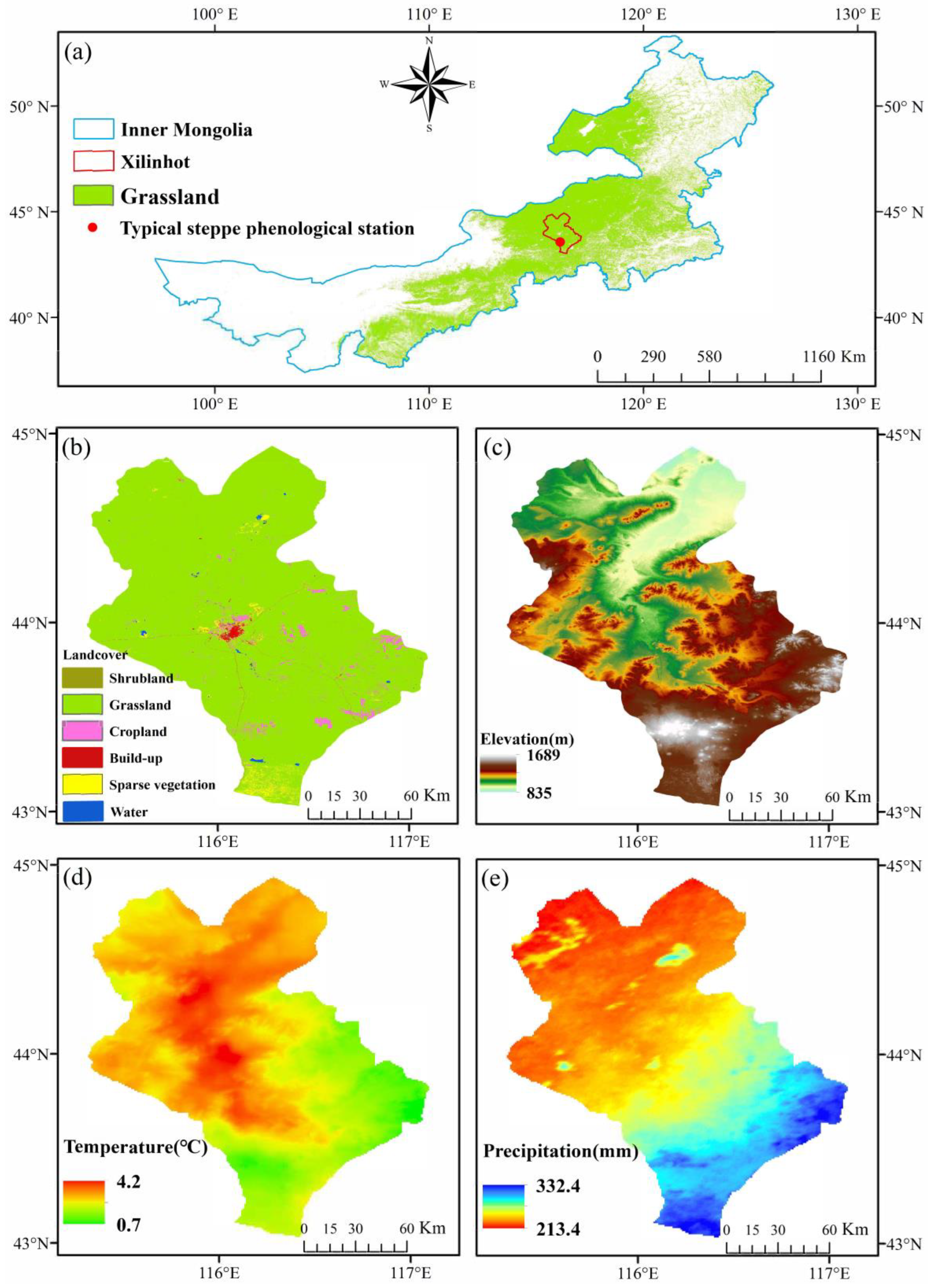
2.1. Study Area

The Inner Mongolia region of China has typical temperate grassland vegetation ecosystems, comprising meadow steppe, typical steppe, desert steppe, and steppe desert types, spanning approximately 13%, 28%, 12%, and 6% of the total area, respectively [42]. The distribution of grassland cover in the region is illustrated in Figure 1a. Xilinhot, which is a typical temperate semi-arid continental climate zone, located in the central-eastern part of Inner Mongolia, is predominantly characterized by typical grassland [25], as shown in Figure 1b. Therefore, the Xilinhot region has been chosen as the study area. It is cold and dry in winter and hot and humid in summer. From 2003 to 2022, the mean annual temperature is 2.6 °C, and the mean annual precipitation is 255 mm. The spatial distribution of elevation in the Xilinhot region is characterized as low in the north and high in the south, ranging primarily between 800 and 1600 m, as shown in Figure 1c. The spatial distribution of the mean temperature from 2000 to 2022 closely corresponds to elevation distributions in the region, where higher elevations are associated with lower mean temperature, as illustrated in Figure 1d. The spatial distribution of the mean precipitation from 2000 to 2022 exhibits irregular patterns, with a prevailing trend of higher precipitation in the southern regions relative to the northern regions, as depicted in Figure 1e.

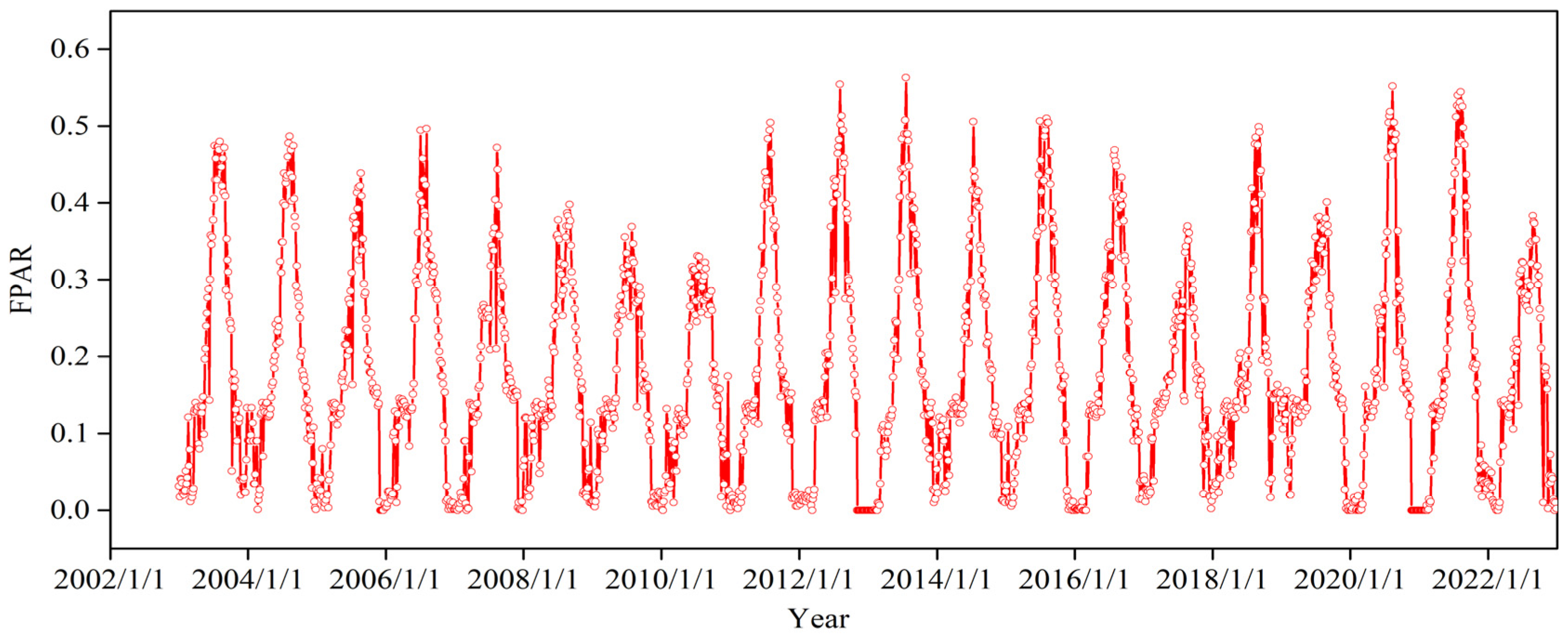
2.2. Data Sources

The land use classification data for Xilinhot originated from the European Space Agency’s (ESA) WorldCover 10 m 2020 v100 product, which was based on Sentinel-1 and Sentinel-2 data and provided a global land cover map for 2020 with a 10 m resolution. The product was acquired through the utilization of the Google Earth Engine (GEE) platform (https://developers.google.cn (accessed on 15 July 2023)). The meteorological data originated from the National Earth System Science Data Center of the National Science and Technology Infrastructure Platform (http://www.geodata.cn (accessed on 10 December 2023)), encompassing monthly mean temperature and precipitation data spanning the period from 2000 to 2022, with a spatial resolution of 0.0083° (approximately 1 km).

Ground-based phenology observations from 2003 to 2022 were obtained at the natural pasture observation site of the Xilinhot National Climate Observatory, Inner Mongolia, China Meteorological Administration, the geographical location of which is shown in the map (Figure 1a). S. krylovii and L. chinensis are two typical dominant species in this region, and C. squarrasa, A. frigida, A. anisopodium and A. tenuissimum are associated species. The EOSs of these species were recorded according to the observation criteria. When 50% of individual herbaceous plants in the plot turn yellow (approximately two-thirds of the plant turns yellow), the period was judged to be the EOS [43]. Moreover, remote sensing data for FPAR based on MODIS (MCD15A3H.006) was obtained using the GEE platform, featuring a spatial resolution of 500 m and a temporal resolution of 4 days. In this study, meteorological data with a spatial resolution of 1000 m are resampled to 500 m to ensure their consistency with remote sensing data. FPAR is primarily derived using a physical model algorithm [44], and this indicator structurally represents the photosynthetic capacity of vegetation. Given the availability of comprehensive observational data for FPAR since 2003, the study period from 2003 to 2022 was chosen. The interannual variation characteristics of FPAR in the typical grassland vegetation of Xilinhot from 2003 to 2022 is depicted (Figure 2). It was apparent that FPAR exhibited varying characteristics across different years, reflecting the vegetation growth conditions of each year. It can be observed that the vegetation condition deteriorated gradually from 2003 to 2010, with improvement noted after 2011.

2.3. Inversion and Analysis Methods of the EOS

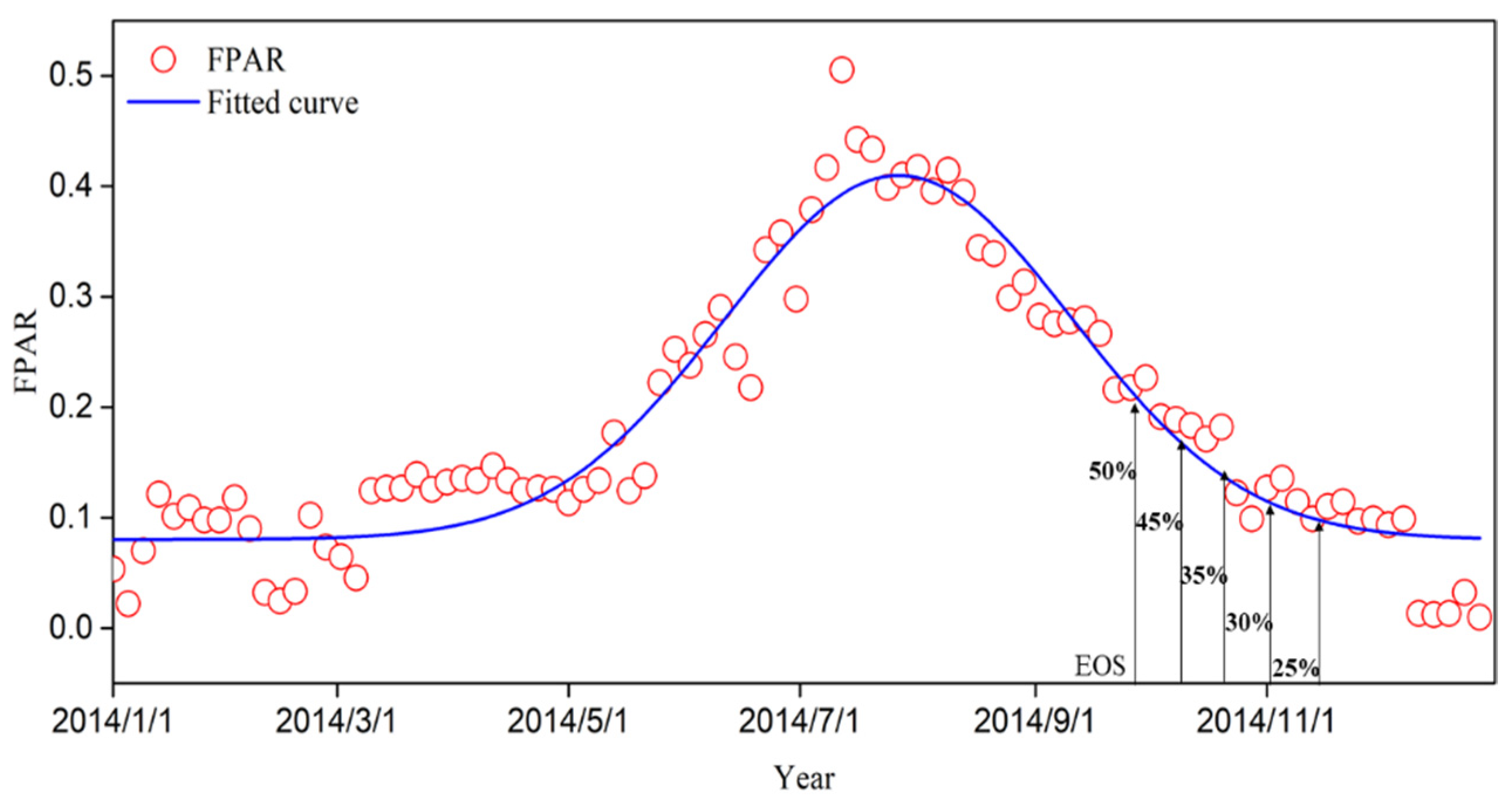
2.3.1. Inversion Method of the EOS

In this study, the vegetation EOS was extracted using TIMESAT 3.3 software, which comprised two key steps. Initially, this study utilized the asymmetric Gaussian (AG) filtering method to reconstruct the time series FPAR curve (Figure 3). Subsequently, the EOS was extracted using the dynamic threshold method based on the reconstructed FPAR time series. The dynamic threshold method, based on the seasonal growth curve in time series data [45], was widely utilized [46,47]. Since the optimal threshold for extracting the EOS of typical grassland vegetation has not been established, this study conducted extensive testing to select the best threshold for extracting the EOS of the semi-arid grassland vegetation. In this study, five thresholds of the EOS were set: 25%, 30%, 35%, 45%, and 50%. To evaluate the accuracy of remote sensing inversion in the EOS, it was compared with ground observation results, and the accuracy was evaluated by the correlation coefficient (r) and p-value. Simultaneously, the Root Mean Square Error (RMSE) for the EOS estimation using different thresholds was determined (Equation (1)). The threshold corresponding to the minimum RMSE value was selected as the optimal threshold for the EOS estimation. Based on the optimal threshold, the spatiotemporal patterns of the EOS in typical grassland vegetation were examined.

$$RMSE=\sqrt{{\displaystyle \frac{1}{n}}{\displaystyle \sum _{j=1}^n{EOS}_{observation}-{EOS}_{simulation}}}$$

(1)

2.3.2. Analysis Method of Spatiotemporal Variation in the EOS

Theil–Sen (TS) median slope trend analysis was used to examine the time trend of the dataset. This method avoids the effects of missing data and data distribution patterns on the analysis results and eliminates the influence of outliers. The formula for this analysis is as follows:

$$\beta =\mathrm{median}({\displaystyle \frac{x_j-x_i}{j-i}}), \forall j>i$$

(2)

where x_i and x_j represent the values for the years i and j, respectively. β represents the trend of the series: positive (delayed) when β > 0, negative (advanced) when β < 0, and insignificant when β = 0.

The time series trend was calculated using the non-parametric Mann–Kendall test. The significance of the TS median slope value was tested using the non-parametric Mann–Kendall test to obtain the Z-score, providing information on trend significance and direction [48]. A positive slope (Z ≥ 1.96) over time indicates a significant delay, while a negative slope (Z ≤ −1.96) indicates a significant advance. For the sequence x_t = x₁, x₂, …, x_n, the magnitude of the relationship between x_i and x_j (set as S) is initially determined for all pairs of values (x_i, x_j, j > i), and the test statistic S is then computed as

$$S={\displaystyle \sum _{i=1}^{n-1}{\displaystyle \sum _{j=i+1}^n\mathit{sgn}(x_j-x_i)}}$$

(3)

In Equation (3), sgn() denotes the sign function and is calculated as

$$sgn(x_j-x_i)=\left\{\begin{array}{ll}1& (x_j-x_i>0)\\ 0& (x_j-x_i=0)\\ -1& (x_j-x_i<0)\end{array}\right.$$

(4)

Equation (5) uses the test statistic Z for trend analysis, and the Z value is calculated as

$$Z=\left\{\begin{array}{ll}{\displaystyle \frac{S}{\sqrt{Var(S)}}}& (S>0)\\ 0& (S=0)\\ {\displaystyle \frac{S+1}{\sqrt{Var(S)}}}& (S<0)\end{array}\right.$$

(5)

In Equation (5), Var is calculated as follows:

$$Var(S)={\displaystyle \frac{n(n-1)(2n+5)}{18}}$$

(6)

2.3.3. Response of the EOS to Climate Change

In this study, the monthly mean temperature and total precipitation in the first three months of the EOS were selected as climate influences to analyze the lag effect of hydrothermal factors on the EOS. The lag effect refers to the use of 1-month scale climatic factors, of which 1-month lag indicates the influence of climatic factors on the EOS in the first month of the preseason, and 3-month lag indicates the influence of climatic factors on the EOS in the third month of the preseason. The lag effect was determined by the lag time scales between the EOS and the climatic factor and its corresponding maximum partial correlation coefficients. The time series (1 ≤ i ≤ 3) of the EOS and climate factors from 2003 to 2022 were constructed, and the partial correlation coefficients of three time series were calculated (the significance level was set to p < 0.05). Three partial correlation coefficients of each pixel were obtained by analyzing the correlation between climatic factors of preseason three months and the EOS. The maximum value of the three partial correlation coefficients was taken as the lag maximum partial correlation coefficient, and its corresponding lag time scale was recorded.

$$R_{lagi}=corr(x_i,y|z_i), 1\le i\le 3$$

(7)

$$R_{\mathit{max}\_lagm}=\mathit{max}(|R_{lagi}|) 1\le i\le 3$$

(8)

where i is the lag time of the i-th month, x_i is the time series of climatic factors before the i-th month of the EOS, y is the EOS time series, z_i is the z value before the i-th month, R_lagi is the lag partial correlation coefficient between y and x_i after controlling z_i, and R_{max_lagm} is the maximum value of R_lagi.

3. Results

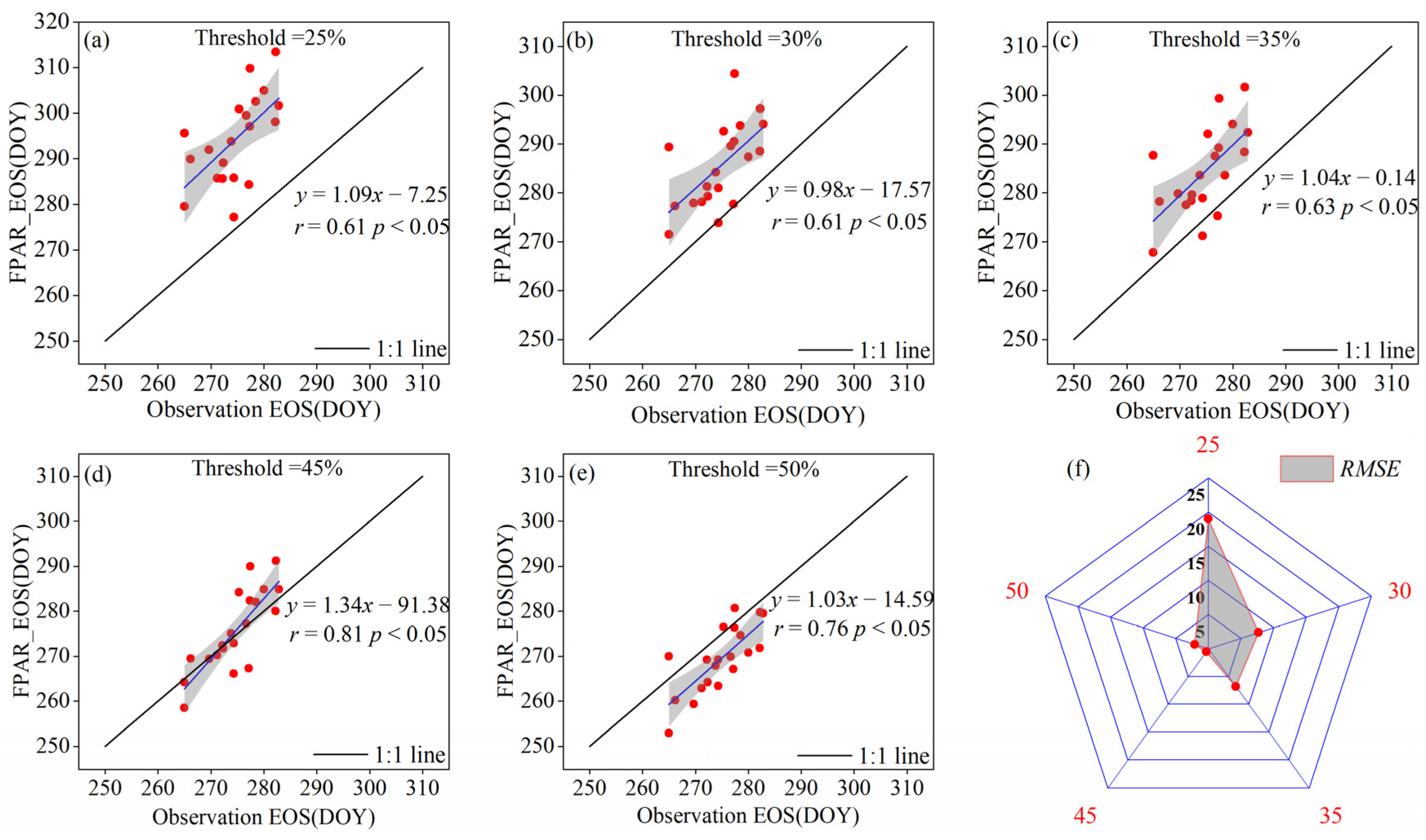
3.1. Dynamic Thresholds for the EOS of Typical Grassland Vegetation

We established the optimal threshold for the remote sensing inversion of the vegetation EOS based on the average occurrence time of multiple measured dominant species’ EOSs. A significant correlation was found between ground-observed EOS and FPAR inversion EOS (p < 0.05) (Figure 4a–e). FPAR inversion of the EOS showed varying RMSEs with different thresholds. The worst accuracy, with the RMSE of 24 days, occurred at a 25% threshold (Figure 4f). The accuracy of the FPAR inversion of vegetation phenology improved with increasing dynamic thresholds, notably at 45% and 50% thresholds, showing RMSEs of 5.5 days (r = 0.81) and 7.1 days (r = 0.76), respectively (Figure 4d–f). This study suggested that 45% threshold was optimal for remote sensing inversion of the EOS of typical grassland vegetation in the semi-arid region.

3.2. Temporal Dynamic Pattern of the EOS of Typical Grassland Vegetation

In this study, the temporal dynamic patterns of ground-based EOS observations from multiple dominant species in typical grasslands and FPAR inversion EOS from 49 spatial points with different altitude ranges (900–1600 m) selected from the study area from 2003 to 2022 were statistically analyzed from 2003 to 2022 (Figure 5a,c). The trend of the EOS for typical grassland vegetation in the semi-arid region from 2003 to 2022 was not readily discernible. However, it exhibited a distinct phase change characteristic, with a reversal phenomenon of advancement followed by postponement. Specifically, the vegetation EOS retrieved by remote sensing showed a reversal phenomenon in the semi-arid region, with significant advancement observed from 2003 to 2011 (p ≤ 0.05), and significant postponement from 2011 to 2022 (p < 0.05) (Figure 5b,d). Overall, these findings demonstrated a temporal dynamic pattern of the EOS in typical grassland vegetation, which was characterized by advance and then delay.

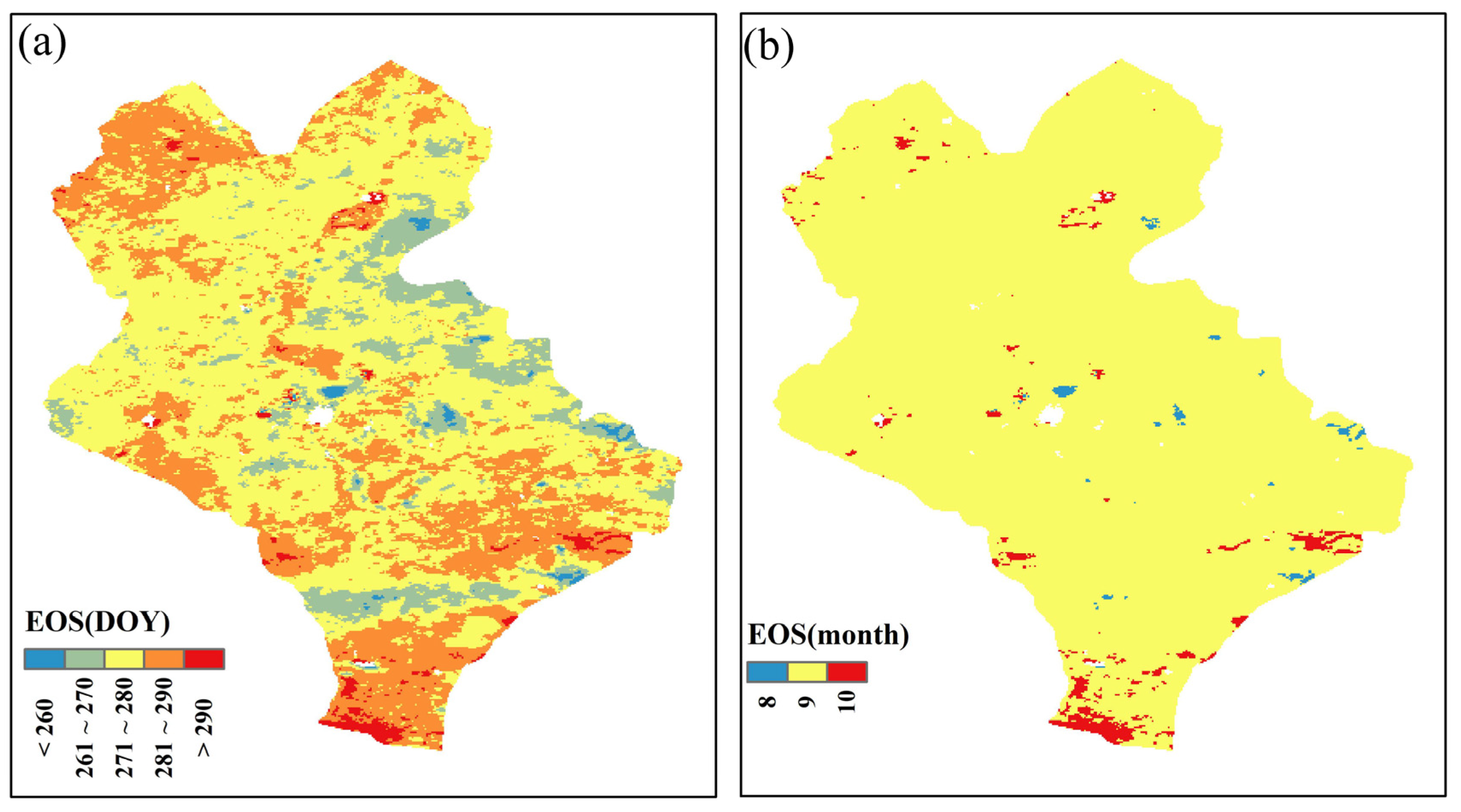
3.3. Spatial Pattern of the EOS of Typical Grassland Vegetation

Firstly, the statistical analysis revealed the average annual spatial distribution of the vegetation EOS of typical grassland vegetation in the semi-arid region (Figure 6). From 2003 to 2022, the EOS was spatially heterogeneous (Figure 6a). The EOS occurred mainly in late September and early October. Based on the discriminatory criteria of classifying the EOS as the previous month if it occurred before the 15th day of the month and classifying the EOS as the current month if it was more than 15 days, the results were as shown in Figure 6b. It can be found that the EOS basically occurred in September.

The research examined the spatial dynamics of the EOS and its implications in three temporal phases (2003–2022, 2003–2011, 2011–2022) by evaluating the extended trend of the EOS spanning from 2003 to 2022 (Figure 7). The analysis indicated that from 2003 to 2022, the proportion of advancing or postponing trend pixels of the EOS was relatively close, and the spatial trend was dominated by a minor postponement (Figure 7a,b). During the period of 2003–2011, the EOS in the eastern part of Xilinhot showed an advance trend, accounting for more than 60% of the trend distribution in the entire study area, with a mainly insignificant advancement during this period (Figure 7c,d). During the period of 2011–2022, the EOS predominantly showed a delayed trend, accounting for more than 90% of the pixels in the study area. In particular, the proportion of the pixels with a significantly delayed trend of the EOS in the northern and central parts of Xilinhot increased significantly (Figure 7e,f). This suggested that the EOS displayed obvious phase change characteristics spatially, and the EOS showed a spatial reversal phenomenon that was first advancing and then delaying.

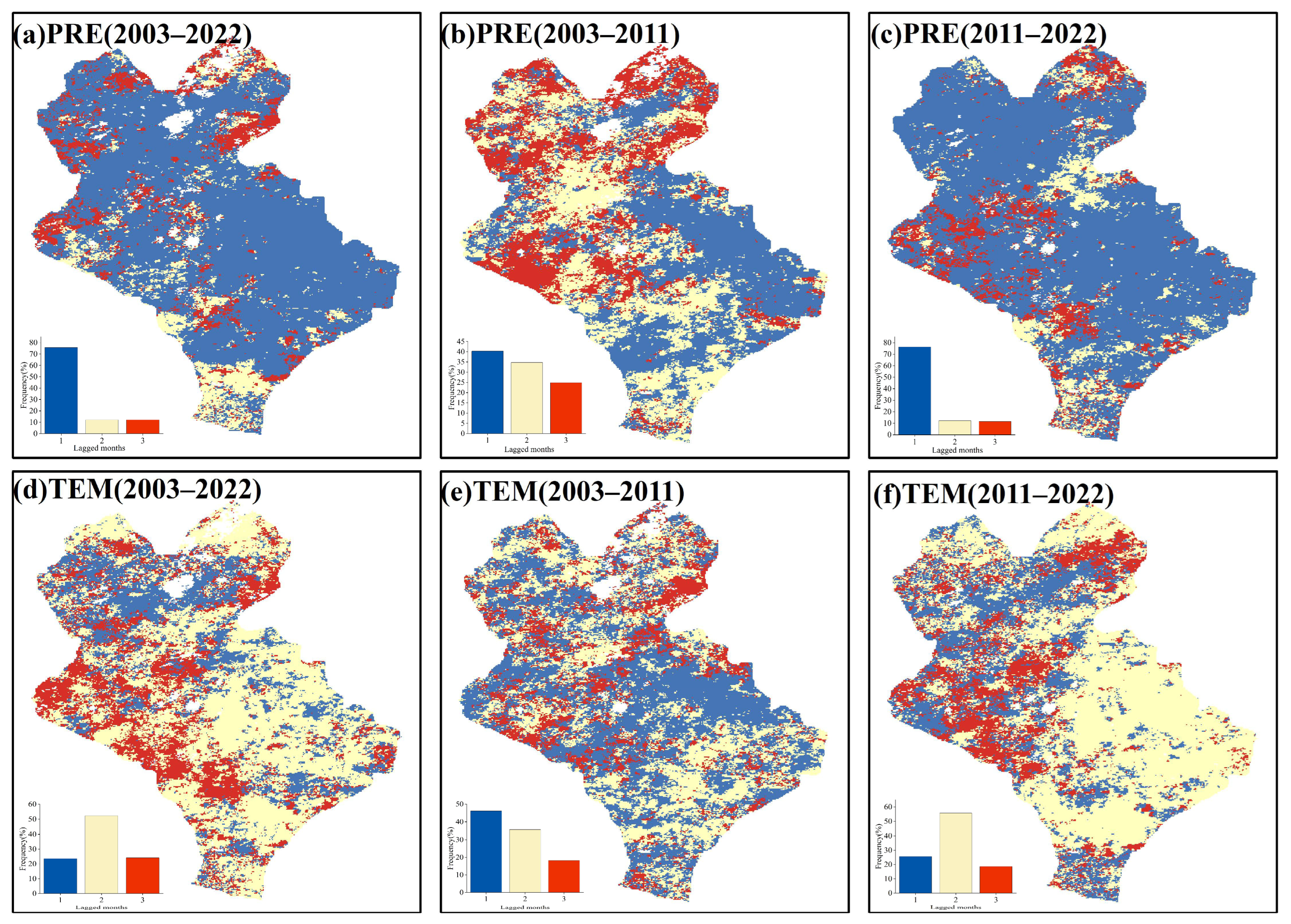
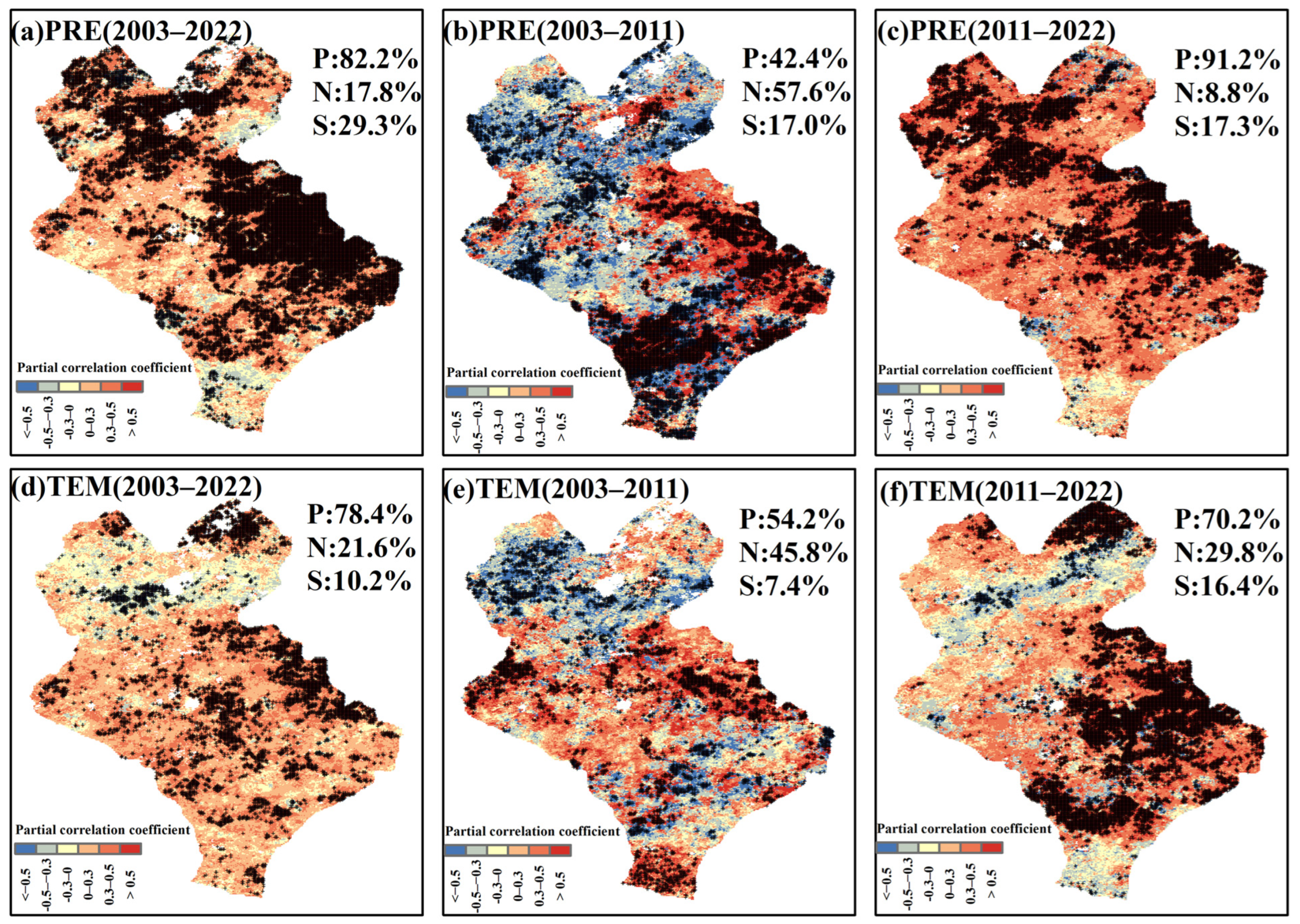
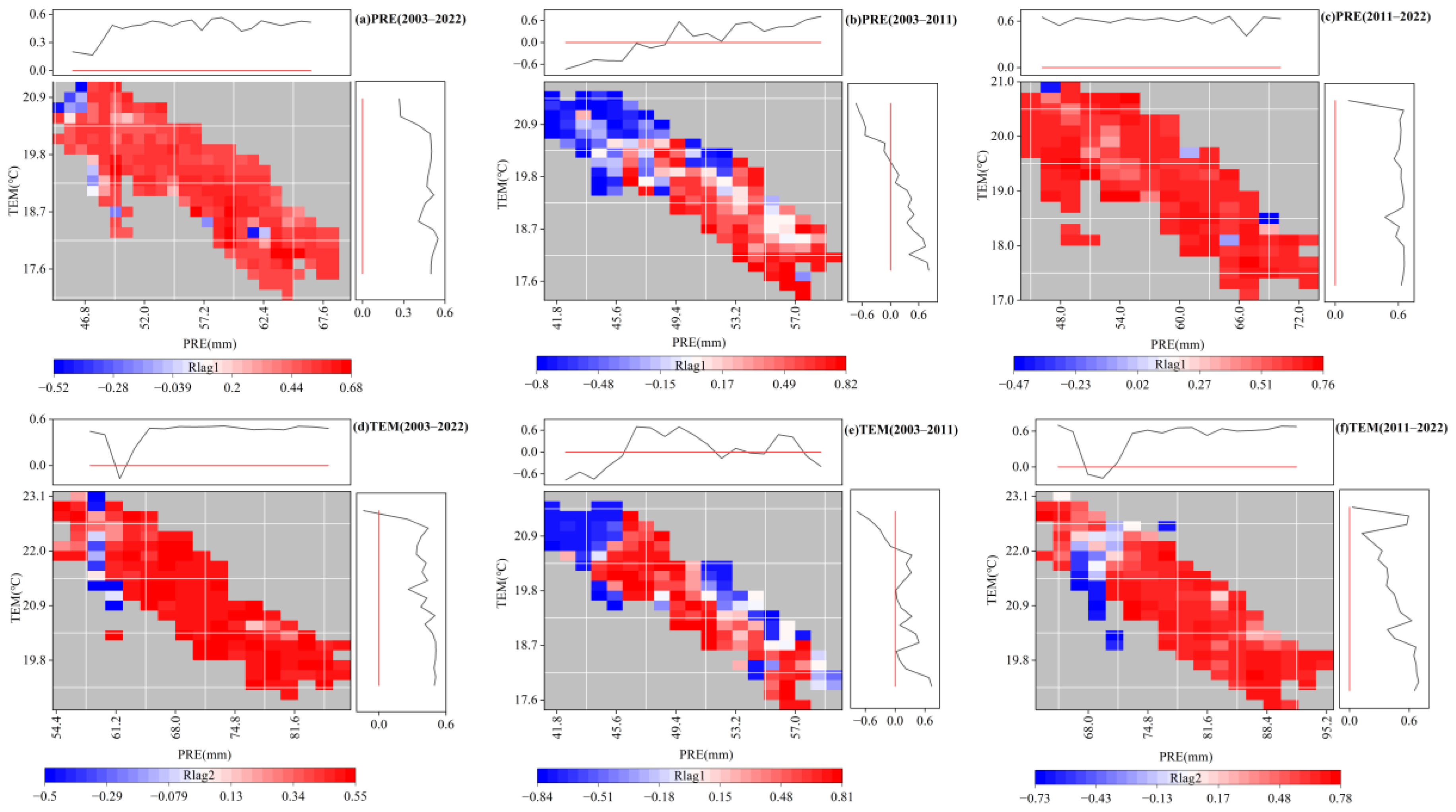
3.4. Response of the EOS to Temperature and Precipitation

The lag response of the EOS to the hydrothermal factors in the three preseason months was explored. The spatial distributions of the lag time scales of vegetation EOS in response to precipitation and temperature were obtained. The spatial heterogeneity of the lag effect of hydrothermal factors on the EOS was strong (Figure 8). For the lag effect of precipitation on the EOS, the lag time scale was dominated by 1 month from 2003 to 2022, and its proportion reached more than 70%. Among them, the lag time scale was dominated by 1 month from 2003 to 2011, while the proportion of the pixels only accounted for 40%, which was mainly distributed in the eastern part of Xilinhot. In addition, the proportion of the pixels with precipitation lag time scales greater than 1 month increased significantly during this period. Similarly, the lag time scale for the EOS response to precipitation was dominated by 1 month from 2011 to 2022, with the proportion of the pixels reaching over 70%. For the lag effect of temperature on the EOS, the lag time scale was mainly 2 months from 2003 to 2022, and its proportion was more than 50%. In particular, the lag time scale was dominated by 1 month from 2003 to 2011, while the proportion of the pixels larger than 1 month was higher than in other time periods. The lag time scale from 2011 to 2022 was dominated by 2 months, with the proportion of the pixels more than 70%. In conclusion, the lag time scales of precipitation and temperature in response to EOS were dominated by 1 month and 2 months, respectively, suggesting that the EOS responded more quickly to short-term precipitation.

The spatial distribution of the maximum lag partial correlation coefficients showed that the lag effects of precipitation and temperature on the EOS changed with different climatic backgrounds (Figure 9). From 2003 to 2022, the lag effects of precipitation and temperature on the EOS were mainly positive, with the proportion of the pixels amounting to 82.2% and 78.4%, respectively (Figure 9a,d). Among them, 29.3% of the pixels passed the significance test for the lag effect of precipitation on the EOS (p < 0.05), which was significantly higher than that of temperature (10.2%), and the significant pixels were mainly located in the eastern part of Xilinhot. The lag effect of precipitation on the EOS from 2003 to 2011 was predominantly negative (57.6%), and that of temperature on the EOS was predominantly positive (54.2%) (Figure 9b,e). The lag effects of precipitation and temperature on the EOS in 2011–2022 were both predominantly positive, and the proportions of the pixels were 91.2% and 70.2%, respectively (Figure 9c,f). In a word, the negative lag effects of both temperature and precipitation on the EOS increased in the climatic context of decreasing precipitation. Temperature had a predominantly positive lag effect on the EOS in the climatic context of increased precipitation. Precipitation was a necessary condition for temperature to delay the EOS of typical grassland vegetation in the semi-arid region.

The overall distribution of the maximum positively partial correlation coefficients of precipitation and temperature lagging by 1–3 months at different periods was statistically analyzed (Figure 10). The distribution of positively partial correlation coefficients between the EOS and precipitation with a lag of 1 month (August) was concentrated and most strongly correlated (Figure 10a). The positively partial correlation coefficients gradually decreased with a longer lag time scale. The positively partial correlation coefficients between the EOS and temperature were not consistent at different periods (Figure 10b), and the distribution of positively partial correlation coefficients between the EOS and temperature with a lag of 2 months (July) was concentrated and the strongest in the context of increasing precipitation from 2011 to 2022. In general, the positive lag effect of precipitation on the EOS gradually weakened with the extension of the lag time scale. Under the background of increasing precipitation, the positive lag effect of temperature lagging for 2 months on the EOS was the strongest.

Based on the above analysis, the distribution of the lag maximum partial correlation coefficients under the precipitation and temperature gradient were further explored (Figure 11). For the precipitation partial correlation coefficients (Figure 11a–c), the partial correlation coefficients for 2003–2022 and 2011–2022 were greater than zero, which indicates that under the current temperature and precipitation gradient, the increase in precipitation and temperature was conducive to the delay of the EOS. Interestingly, at the stage of decreasing precipitation from 2003 to 2011, the partial correlation coefficients changed from positive to negative with the increase in temperature and from negative to positive with the increase in precipitation. This indicates that under the climatic background of this stage, the increase in precipitation exceeding a certain value was beneficial to the delay of the EOS, and the increase in temperature exceeding a certain value was not conducive to the delay of the EOS. For the temperature partial correlation coefficients, the partial correlation coefficients changed from positive to negative with the increase in temperature from 2003 to 2011, which indicated that the increase in temperature at this stage to a certain extent was not conducive to the delay of the EOS. In general, satisfying precipitation was a prerequisite for temperature to delay the EOS, and the climatic background played an important role in regulating the response of typical steppe vegetation to hydrothermal factors in the semi-arid region.

4. Discussion

4.1. Thresholds for Remote Sensing Inversion of Vegetation EOS

Extensive research has been conducted on vegetation phenology retrieval by remote sensing [49]. However, the accuracy of phenological inversion still needs to be further improved. The accuracy of the remote sensing inversion of vegetation phenology relies on the selection of the time series reconstruction method and the phenology extraction method [45]. However, the spatiotemporal resolutions of remote sensing data sources are also crucial factors influencing the accuracy of phenology extraction [32]. In this study, FPAR, which served as an ecological remote sensing indicator with high spatial and temporal resolution, was utilized to invert the vegetation EOS of typical grassland in the semi-arid region. The inversion accuracy generally surpassed that of existing studies, with an RMSE of 5.5 days and an r of 0.81. Numerous studies have demonstrated that the dynamic threshold method gives better inversion results for vegetation phenology [45]. Moreover, the current study determined the vegetation EOS in the study area utilizing this method. Furthermore, this study established the threshold (45%) of the vegetation EOS using this method, thereby offering a reference for further research on the remote sensing inversion of the vegetation EOS in typical grassland. Additionally, the dynamic thresholds varied across vegetation types and study areas [32,45,48,50]. Hence, it is essential to elucidate the optimal threshold for remote sensing inversion of various vegetation types, as this is crucial for accurately inverting the vegetation EOS of different vegetation types. Although the dynamic threshold method is widely used, it should be noted that the threshold setting in the dynamic threshold method relies on experience and subjectivity. It is necessary to set multiple potential thresholds to complete the inversion of vegetation phenology.

4.2. Response Mechanism of Grassland Vegetation EOS to Climate Change

Prior studies have commonly asserted that temperature primarily determines vegetation phenology [51]. However, elucidating the response of phenology to environmental shifts solely through temperature regulation proved challenging [52]. For instance, research indicated that both temperature and precipitation played essential roles in regulating vegetation phenology in the semi-arid region. Specifically, heightened summer precipitation and autumn temperature were crucial for postponing the EOS in a temperate grassland ecosystem [9]. This study observed positive correlations between preseason temperature, precipitation, and the EOS, aligning with findings from previous studies [28,47]. Especially in the context of increased precipitation, the positive effect of temperature was more obvious. This relationship could be attributed to elevated temperature boosting photosynthetic enzyme activity and decelerating the decomposition of chlorophyll, consequently prolonging the EOS [38,53]. Studies indicated that preseason precipitation exerted a more substantial impact on the EOS than temperature for grassland vegetation in arid regions [28,41,54]. We found that the lag time scales of precipitation and temperature to the EOS were mainly 1 month and 2 months, respectively. Moreover, precipitation was proposed as the primary climatic factor influencing the EOS of grassland vegetation [29,55], possibly linked to water stress effects on autumnal plant growth. This study suggested that the shift in spatiotemporal patterns of the EOS in the semi-arid typical grassland was predominantly associated with augmented precipitation and that a 1 month lag in precipitation dominated the postponement of the EOS. The link between heightened precipitation and delayed EOS was likely due to enhanced water efficiency [56,57]. Conversely, in the Tibetan Plateau region, the herbaceous plant EOS occurred earlier and was more sensitive to temperature as precipitation increased [36]. This phenomenon was likely due to the combination of abundant precipitation and extremely cold temperature at high elevations, rendering temperature a constraining factor for alpine grassland growth. These variations implied significant diversity in climate–vegetation relationships among regions and vegetation types [58,59], highlighting the intricate and variable nature of vegetation phenological responses to climate change [60,61]. Moreover, they indicated that the influences of temperature and precipitation on grassland vegetation phenology were interdependent rather than independent, with each factor constraining the other [62]. Furthermore, climate fluctuations during specific critical periods can exert more pronounced effects on vegetation phenology [63]. For instance, heightened precipitation in August can prolong the EOS [42]. Precipitation in August has emerged as a significant constraint on vegetation growth in the Tibetan Plateau region [64]. Moreover, the current study unambiguously identifies precipitation in August as the primary climatic determinant limiting the EOS of typical grassland vegetation in the semi-arid region, corroborating the importance of precipitation in shaping vegetation growth in arid and semi-arid ecosystems [54].

4.3. Limitations and Future Research

In this study, there are some limitations. Firstly, only one ground phenological observation site was used as a reference for the ground phenological verification of remote sensing inversion of vegetation phenology. On the one hand, more ground observation data of different species in different geographical locations need to be collected. On the other hand, current research mainly used simple averages of ground observations of the phenology of one or several species to verify the accuracy of remotely sensed vegetation phenology. There are significant differences in remote sensing vegetation phenology estimated by different methods, and no method can fully reproduce the ground observation of vegetation phenology for different vegetation types. The combination of ground-based and remotely sensed vegetation phenology has great potential to address the issue of scaling between individual species and ecosystem responses. Another limitation of this study is that the effect of soil moisture was not excluded from the identification of the effect of precipitation on vegetation phenology. Intra-annual precipitation patterns determine the availability of soil moisture at critical plant growth stages, suggesting that soil moisture at specific times may have outsized impacts on the EOS [35,57,65]. Soil moisture is a more straightforward driving factor for vegetation phenology than precipitation [66]. Therefore, decoupling the influence of precipitation and soil moisture on vegetation phenology and their contributions are critical for understanding and constructing vegetation phenology models.

The rising frequency of extreme events with climate warming heightens uncertainty in forecasting the impacts of climate change on ecosystems [67,68]. Research indicated that extreme events exerted more direct and pronounced effects on vegetation phenology compared to average climate change [69]. Extreme events were more effective in explaining the EOS compared to mean climate conditions [56]. Consequently, it is challenging to explain changes in phenology by relying solely on the average climate states. For instance, extreme drought delayed the plant green-up date by 6–34 days compared to the average multi-year green-up date, consequently advancing the EOS by approximately 12 days. Currently, extreme events have received relatively little attention, leading to a significant gap in our understanding of the climate response mechanisms governing vegetation phenology [69,70]. To comprehend the response of complex grassland phenology to climate change, future research shall delve into the mechanisms underlying the synergistic effects of mean climate conditions and extreme events on vegetation phenology. Additionally, the compounded impact of multiple extreme events on ecosystems often surpasses the effect of individual extreme events. For instance, in the Qilian Mountains, the plant green-up date was advanced by 6.4 days and 5.1 days during years of extreme heat and extreme wetness, respectively, whereas the combination of warm and wet events accelerated the plant green-up date by 13.2 days. Nonetheless, the interaction between multiple extreme events and their collective influence on plant phenology during compound extreme events remains poorly understood. Urgent future research is required to disentangle the effects of compound extreme events on plant phenology into individual extreme events. Field experiments are imperative for gaining mechanistic insights into the response mechanisms of vegetation dieback to both mean climate conditions and extreme climate events [28,56].

5. Conclusions

The study utilized the time series of the Fraction of Absorbed Photosynthetically Active Radiation (FPAR) for MODIS spanning from 2003 to 2022. The time series were filtered by an asymmetric Gaussian filtering algorithm, and the optimal threshold for identifying the typical grassland vegetation EOS was determined through the dynamic threshold method. The research unveiled the spatiotemporal patterns of the EOS of typical grassland vegetation in the semi-arid region and its response to climate change. Over the past two decades, there has been a reversal in the spatiotemporal patterns of the EOS. Increased precipitation in August was the primary factor influencing the occurrence of the EOS in the region. Increased precipitation played a key role in reversing the EOS of typical grassland vegetation, and its effect on postponing the EOS was more pronounced than that of temperature. The dynamic threshold for inversion of the EOS in this study will provide an important reference for future research. In addition, it was found that precipitation is the main climatic factor controlling the EOS, which must be taken into account in the phenological model.

References

- Ren, S.L.; Yi, S.H.; Peichl, M.; Wang, X.Y. Diverse responses of vegetation phenology to climate change in different grasslands in Inner Mongolia during 2000–2016. Remote Sens. 2017, 10, 17. [Google Scholar] [CrossRef]
- Li, Q.Y.; Xu, L.; Pan, X.B.; Zhang, L.Z.; Li, C.; Yang, N.; Qi, J.G. Modeling phenological responses of Inner Mongolia grassland species to regional climate change. Environ. Res. Lett. 2016, 11, 015002. [Google Scholar] [CrossRef]
- Czernecki, B.; Nowosad, J.; Jablonska, K. Machine learning modeling of plant phenology based on coupling satellite and gridded meteorological dataset. Int. J. Biometeorol. 2018, 62, 1297–1309. [Google Scholar] [CrossRef] [PubMed]
- Xin, Q.C.; Broich, M.; Zhu, P.; Gong, P. Modeling grassland spring onset across the Western United States using climate variables and MODIS-derived phenology metrics. Remote Sens. Environ. 2015, 161, 63–77. [Google Scholar] [CrossRef]
- Bao, G.; Chen, J.Q.; Chopping, M.; Bao, Y.H.; Bayarsaikhan, S.; Dorjsuren, A.; Tuya, A.; Jirigala, B.; Qin, Z.H. Dynamics of net primary productivity on the Mongolian Plateau: Joint regulations of phenology and drought. Int. J. Appl. Earth Obs. Geoinf. 2019, 81, 85–97. [Google Scholar] [CrossRef]
- D’Odorico, P.; Gonsamo, A.; Gough, C.M.; Bohrer, G.; Morison, J.; Wilkinson, M.; Hanson, P.J.; Gianelle, D.; Fuentes, J.D.; Buchmann, N. The match and mismatch between photosynthesis and land surface phenology of deciduous forests. Agric. For. Meteorol. 2015, 214–215, 25–38. [Google Scholar] [CrossRef]
- Richardson, A.D.; Black, T.A.; Ciais, P.; Delbart, N.; Friedl, M.A.; Gobron, N.; Hollinger, D.Y.; Kutsch, W.L.; Longdoz, B.; Luyssaert, S.; et al. Influence of spring and autumn phenological transitions on forest ecosystem productivity. Philos. Trans. R. Soc. Lond. B Biol. Sci. 2010, 365, 3227–3246. [Google Scholar] [CrossRef]
- Meng, F.D.; Zhang, L.R.; Zhang, Z.H.; Jiang, L.L.; Wang, Y.F.; Duan, J.H.; Wang, Q.; Li, B.W.; Liu, P.P.; Hong, H.; et al. Enhanced spring temperature sensitivity of carbon emission links to earlier phenology. Sci. Total Environ. 2020, 745, 140999. [Google Scholar] [CrossRef]
- Ma, R.; Shen, X.; Zhang, J.; Xia, C.; Liu, Y.; Wu, L.; Wang, Y.; Jiang, M.; Lu, X. Variation of vegetation autumn phenology and its climatic drivers in temperate grasslands of China. Int. J. Appl. Earth Obs. Geoinf. 2022, 114, 103064. [Google Scholar] [CrossRef]
- Ahas, R.; Aasa, A.; Menzel, A.; Fedotova, V.G.; Scheifinger, H. Changes in European spring phenology. Int. J. Climatol. 2002, 22, 1727–1738. [Google Scholar] [CrossRef]
- Fang, X.Q.; Chen, F.H. Plant phenology and climate change. Sci. China Earth Sci. 2015, 58, 1043–1044. [Google Scholar] [CrossRef]
- Ma, T.; Zhou, C.H. Climate-associated changes in spring plant phenology in China. Int. J. Biometeorol. 2011, 56, 269–275. [Google Scholar] [CrossRef] [PubMed]
- Zhou, X.C.; Geng, X.J.; Yin, G.D.; Hänninen, H.; Hao, F.H.; Zhang, X.; Fu, Y.H. Legacy effect of spring phenology on vegetation growth in temperate China. Agric. For. Meteorol. 2020, 281, 107845. [Google Scholar] [CrossRef]
- Liu, Q.; Fu, Y.H.; Zhu, Z.C.; Liu, Y.W.; Liu, Z.; Huang, M.T.; Janssens, I.A.; Piao, S.L. Delayed autumn phenology in the Northern Hemisphere is related to change in both climate and spring phenology. Glob. Chang. Biol. 2016, 22, 3702–3711. [Google Scholar] [CrossRef] [PubMed]
- Sun, Q.L.; Li, B.L.; Zhou, G.Y.; Jiang, Y.H.; Yuan, Y.C. Delayed autumn leaf senescence date prolongs the growing season length of herbaceous plants on the Qinghai–Tibetan Plateau. Agric. For. Meteorol. 2020, 284, 107896. [Google Scholar] [CrossRef]
- Shen, X.J.; Liu, B.H.; Henderson, M.; Wang, L.; Wu, Z.F.; Wu, H.T.; Jiang, M.; Lu, X.G. Asymmetric effects of daytime and nighttime warming on spring phenology in the temperate grasslands of China. Agric. For. Meteorol. 2018, 259, 240–249. [Google Scholar] [CrossRef]
- Zhang, R.P.; Guo, J.; Liang, T.G.; Feng, Q.S. Grassland vegetation phenological variations and responses to climate change in the Xinjiang region, China. Quat. Int. 2019, 513, 56–65. [Google Scholar] [CrossRef]
- Sun, M.; Li, P.; Ren, P.; Tang, J.; Zhang, C.; Zhou, X.; Peng, C. Divergent response of vegetation phenology to extreme temperatures and precipitation of different intensities on the Tibetan Plateau. Sci. China Earth Sci. 2023, 66, 2200–2210. [Google Scholar] [CrossRef]
- Wang, X.F.; Xiao, J.F.; Li, X.; Cheng, G.D.; Ma, M.G.; Zhu, G.F.; Arain, M.A.; Black, T.A.; Jassal, R.S. No trends in spring and autumn phenology during the global warming hiatus. Nat. Commun. 2019, 10, 2389. [Google Scholar] [CrossRef]
- Zhao, J.J.; Zhang, H.Y.; Zhang, Z.X.; Guo, X.Y.; Li, X.D.; Chen, C. Spatial and temporal changes in vegetation phenology at middle and high latitudes of the Northern Hemisphere over the past three decades. Remote Sens. 2015, 7, 10973–10995. [Google Scholar] [CrossRef]
- Li, P.; Peng, C.H.; Wang, M.; Luo, Y.P.; Li, M.X.; Zhang, K.R.; Zhang, D.L.; Zhu, Q.A. Dynamics of vegetation autumn phenology and its response to multiple environmental factors from 1982 to 2012 on Qinghai-Tibetan Plateau in China. Sci. Total Environ. 2018, 637–638, 855–864. [Google Scholar] [CrossRef] [PubMed]
- Yuan, H.H.; Wu, C.Y.; Gu, C.Y.; Wang, X.Y. Evidence for satellite observed changes in the relative influence of climate indicators on autumn phenology over the Northern Hemisphere. Glob. Planet. Chang. 2020, 187, 103131. [Google Scholar] [CrossRef]
- Wang, X.F.; Xiao, J.F.; Li, X.; Cheng, G.D.; Ma, M.G.; Che, T.; Dai, L.Y.; Wang, S.Y.; Wu, J.K. No consistent evidence for advancing or delaying trends in spring phenology on the Tibetan Plateau. J. Geophys. Res. Biogeosci. 2017, 122, 3288–3305. [Google Scholar] [CrossRef]
- Tao, Z.X.; Wang, H.J.; Liu, Y.C.; Xu, Y.J.; Dai, J.H. Phenological response of different vegetation types to temperature and precipitation variations in northern China during 1982–2012. Int. J. Remote Sens. 2017, 38, 3236–3252. [Google Scholar] [CrossRef]
- Ren, S.L.; Chen, X.; An, S. Assessing plant senescence reflectance index-retrieved vegetation phenology and its spatiotemporal response to climate change in the Inner Mongolian Grassland. Int. J. Biometeorol. 2017, 61, 601–612. [Google Scholar] [CrossRef]
- Shen, M.G.; Wang, S.P.; Jiang, N.; Sun, J.P.; Cao, R.Y.; Ling, X.F.; Fang, B.; Zhang, L.; Zhang, L.H.; Xu, X.; et al. Plant phenology changes and drivers on the Qinghai–Tibetan Plateau. Nat. Rev. Earth Environ. 2022, 3, 633–651. [Google Scholar] [CrossRef]
- Miao, L.; Muller, D.; Cui, X.; Ma, M. Changes in vegetation phenology on the Mongolian Plateau and their climatic determinants. PLoS ONE 2017, 12, e0190313. [Google Scholar] [CrossRef]
- Liu, Q.; Fu, Y.H.; Zeng, Z.Z.; Huang, M.T.; Li, X.R.; Piao, S.L. Temperature, precipitation, and insolation effects on autumn vegetation phenology in temperate China. Glob. Chang. Biol. 2016, 22, 644–655. [Google Scholar] [CrossRef]
- Fan, J.; Min, J.; Yang, Q.; Na, J.; Wang, X. Spatial-temporal relationship analysis of vegetation phenology and meteorological parameters in an agro-pasture ecotone in China. Remote Sens. 2022, 14, 5417. [Google Scholar] [CrossRef]
- Wu, C.; Hou, X.; Peng, D.; Gonsamo, A.; Xu, S. Land surface phenology of China’s temperate ecosystems over 1999–2013: Spatial–temporal patterns, interaction effects, covariation with climate and implications for productivity. Agric. For. Meteorol. 2016, 216, 177–187. [Google Scholar] [CrossRef]
- Chen, X.Q.; Li, J.; Xu, L.; Liu, L.; Ding, D. Modeling greenup date of dominant grass species in the Inner Mongolian Grassland using air temperature and precipitation data. Int. J. Biometeorol. 2014, 58, 463–471. [Google Scholar] [CrossRef] [PubMed]
- Zhu, Y.; Zhang, Y.; Zu, J.; Wang, Z.; Huang, K.; Cong, N.; Tang, Z. Effects of data temporal resolution on phenology extractions from the alpine grasslands of the Tibetan Plateau. Ecol. Indic. 2019, 104, 365–377. [Google Scholar] [CrossRef]
- Verstraete, M.M.; Gobron, N.; Aussedat, O.; Robustelli, M.; Pinty, B.; Widlowski, J.-L.; Taberner, M. An automatic procedure to identify key vegetation phenology events using the JRC-FAPAR products. Adv. Space Res. 2008, 41, 1773–1783. [Google Scholar] [CrossRef]
- Garrity, S.R.; Bohrer, G.; Maurer, K.D.; Mueller, K.L.; Vogel, C.S.; Curtis, P.S. A comparison of multiple phenology data sources for estimating seasonal transitions in deciduous forest carbon exchange. Agric. For. Meteorol. 2011, 151, 1741–1752. [Google Scholar] [CrossRef]
- Tao, Z.; Ge, Q.; Wang, H.; Dai, J. The important role of soil moisture in controlling autumn phenology of herbaceous plants in the Inner Mongolian steppe. Land Degrad. Dev. 2020, 32, 3698–3710. [Google Scholar] [CrossRef]
- Zhu, W.; Jiang, N.; Chen, G.; Zhang, D.; Zheng, Z.; Fan, D. Divergent shifts and responses of plant autumn phenology to climate change on the Qinghai-Tibetan Plateau. Agric. For. Meteorol. 2017, 239, 166–175. [Google Scholar] [CrossRef]
- Guo, J.; Yang, X.C.; Niu, J.M.; Jin, Y.X.; Xu, B.; Shen, G.; Zhang, W.B.; Zhao, F.; Zhang, Y.J. Remote sensing monitoring of green-up dates in the Xilingol grasslands of northern China and their correlations with meteorological factors. Int. J. Remote Sens. 2018, 40, 2190–2211. [Google Scholar] [CrossRef]
- Richardson, A.D.; Keenan, T.F.; Migliavacca, M.; Ryu, Y.; Sonnentag, O.; Toomey, M. Climate change, phenology, and phenological control of vegetation feedbacks to the climate system. Agric. For. Meteorol. 2013, 169, 156–173. [Google Scholar] [CrossRef]
- Hänninen, H.; Kramer, K.; Tanino, K.; Zhang, R.; Wu, J.; Fu, Y.H. Experiments are necessary in process-based tree phenology modelling. Trends Plant Sci. 2019, 24, 199–209. [Google Scholar] [CrossRef]
- Gallinat, A.S.; Primack, R.B.; Wagner, D.L. Autumn, the neglected season in climate change research. Trends Ecol. Evol. 2015, 30, 169–176. [Google Scholar] [CrossRef]
- Ma, P.F.; Zhao, J.X.; Zhang, H.Z.; Zhang, L.; Luo, T.X. Increased precipitation leads to earlier green-up and later senescence in Tibetan alpine grassland regardless of warming. Sci. Total Environ. 2023, 871, 162000. [Google Scholar] [CrossRef] [PubMed]
- Sha, Z.; Zhong, J.; Bai, Y.; Tan, X.; Li, J. Spatio-temporal patterns of satellite-derived grassland vegetation phenology from 1998 to 2012 in Inner Mongolia, China. J. Arid. Land 2016, 8, 462–477. [Google Scholar] [CrossRef]
- Liu, E.H.; Zhou, G.S.; He, Q.J.; Wu, B.Y.; Zhou, H.L.; Gu, W.J. Climatic mechanism of delaying the start and advancing the end of the growing season of Stipa krylovii in a semi-arid region from 1985–2018. Agronomy 2022, 12, 1906. [Google Scholar] [CrossRef]
- Dong, T.; Liu, J.; Shang, J.; Qian, B.; Huffman, T.; Zhang, Y.; Champagne, C.; Daneshfar, B. Assessing the impact of climate variability on cropland productivity in the Canadian prairies using time series MODIS FAPAR. Remote Sens. 2016, 8, 281. [Google Scholar] [CrossRef]
- Xu, Y.; Li, X.; Du, H.; Mao, F.; Zhou, G.; Huang, Z.; Fan, W.; Chen, Q.; Ni, C.; Guo, K. Improving extraction phenology accuracy using SIF coupled with the vegetation index and mapping the spatiotemporal pattern of bamboo forest phenology. Remote Sens. Environ. 2023, 297, 113785. [Google Scholar] [CrossRef]
- Bórnez, K.; Descals, A.; Verger, A.; Peñuelas, J. Land surface phenology from VEGETATION and PROBA-V data. Assessment over deciduous forests. Int. J. Appl. Earth Obs. Geoinf. 2020, 84, 101974. [Google Scholar] [CrossRef]
- Zhang, X.; Du, X.; Hong, J.; Du, Z.; Lu, X.; Wang, X. Effects of climate change on the growing season of alpine grassland in Northern Tibet, China. Glob. Ecol. Conserv. 2020, 23, e01126. [Google Scholar] [CrossRef]
- Kang, W.P.; Wang, T.; Liu, S.L. The response of vegetation phenology and productivity to drought in semi-arid regions of Northern China. Remote Sens. 2018, 10, 727. [Google Scholar] [CrossRef]
- Zhou, L.; Zhou, W.; Chen, J.; Xu, X.; Wang, Y.; Zhuang, J.; Chi, Y. Land surface phenology detections from multi-source remote sensing indices capturing canopy photosynthesis phenology across major land cover types in the Northern Hemisphere. Ecol. Indic. 2022, 135, 108579. [Google Scholar] [CrossRef]
- Verger, A.; Filella, I.; Baret, F.; Peñuelas, J. Vegetation baseline phenology from kilometric global LAI satellite products. Remote Sens. Environ. 2016, 178, 1–14. [Google Scholar] [CrossRef]
- Wang, S.Y.; Yang, B.J.; Yang, Q.C.; Lu, L.L.; Wang, X.Y.; Peng, Y.Y. Temporal trends and spatial variability of vegetation phenology over the Northern Hemisphere during 1982–2012. PLoS ONE 2016, 11, e0157134. [Google Scholar] [CrossRef]
- Marchin, R.M.; Salk, C.F.; Hoffmann, W.A.; Dunn, R.R. Temperature alone does not explain phenological variation of diverse temperate plants under experimental warming. Glob. Chang. Biol. 2015, 21, 3138–3151. [Google Scholar] [CrossRef] [PubMed]
- Wu, C.; Wang, X.; Wang, H.; Ciais, P.; Peñuelas, J.; Myneni, R.B.; Desai, A.R.; Gough, C.M.; Gonsamo, A.; Black, A.T.; et al. Contrasting responses of autumn-leaf senescence to daytime and night-time warming. Nat. Clim. Chang. 2018, 8, 1092–1096. [Google Scholar] [CrossRef]
- Currier, C.M.; Sala, O.E. Precipitation versus temperature as phenology controls in drylands. Ecology 2022, 103, e3793. [Google Scholar] [CrossRef] [PubMed]
- Zhou, Y.Z.; Jia, G.S. Precipitation as a control of vegetation phenology for temperate steppes in China. Atmos. Ocean. Sci. Lett. 2016, 9, 162–168. [Google Scholar] [CrossRef]
- Gao, X.; Tao, Z.; Dai, J. Significant influences of extreme climate on autumn phenology in Central Asia grassland. Ecol. Indic. 2023, 155, 111056. [Google Scholar] [CrossRef]
- Luo, M.; Meng, F.H.; Sa, C.L.; Duan, Y.C.; Bao, Y.; Liu, T.; De Maeyer, P. Response of vegetation phenology to soil moisture dynamics in the Mongolian Plateau. Catena 2021, 206, 105505. [Google Scholar] [CrossRef]
- Cong, N.; Piao, S.L.; Chen, A.P.; Wang, X.H.; Lin, X.; Chen, S.P.; Han, S.J.; Zhou, G.S.; Zhang, X.P. Spring vegetation green-up date in China inferred from SPOT NDVI data: A multiple model analysis. Agric. For. Meteorol. 2012, 165, 104–113. [Google Scholar] [CrossRef]
- Zhang, R.; Qi, J.; Leng, S.; Wang, Q. Long-term vegetation phenology changes and responses to preseason temperature and precipitation in northern China. Remote Sens. 2022, 14, 1396. [Google Scholar] [CrossRef]
- Ganjurjav, H.; Gao, Q.; Schwartz, M.W.; Zhu, W.; Liang, Y.; Li, Y.; Wan, Y.; Cao, X.; Williamson, M.A.; Jiangcun, W.; et al. Complex responses of spring vegetation growth to climate in a moisture-limited alpine meadow. Sci. Rep. 2016, 6, 23356. [Google Scholar] [CrossRef]
- Yuan, M.X.; Zhao, L.; Lin, A.W.; Li, Q.J.; She, D.X.; Qu, S. How do climatic and non-climatic factors contribute to the dynamics of vegetation autumn phenology in the Yellow River Basin, China? Ecol. Indic. 2020, 112, 106112. [Google Scholar] [CrossRef]
- Cheng, M.; Wang, Y.; Zhu, J.X.; Pan, Y. Precipitation dominates the relative contributions of climate factors to grasslands spring phenology on the Tibetan Plateau. Remote Sens. 2022, 14, 517. [Google Scholar] [CrossRef]
- Wang, G.C.; Huang, Y.; Wei, Y.R.; Zhang, W.; Li, T.T.; Zhang, Q. Inner Mongolian grassland plant phenological changes and their climatic drivers. Sci. Total Environ. 2019, 683, 1–8. [Google Scholar] [CrossRef]
- Zhang, Q.; Kong, D.D.; Shi, P.J.; Singh, V.P.; Sun, P. Vegetation phenology on the Qinghai-Tibetan Plateau and its response to climate change (1982–2013). Agric. For. Meteorol. 2018, 248, 408–417. [Google Scholar] [CrossRef]
- Wang, X.; Wu, C.; Liu, Y.; Peñuelas, J.; Peng, J. Earlier leaf senescence dates are constrained by soil moisture. Glob. Chang. Biol. 2022, 29, 1557–1573. [Google Scholar] [CrossRef] [PubMed]
- Cui, X.; Xu, G.; He, X.; Luo, D. Influences of Seasonal Soil Moisture and Temperature on Vegetation Phenology in the Qilian Mountains. Remote Sens. 2022, 14, 3645. [Google Scholar] [CrossRef]
- He, Z.B.; Du, J.; Chen, L.F.; Zhu, X.; Lin, P.F.; Zhao, M.M.; Fang, S. Impacts of recent climate extremes on spring phenology in arid-mountain ecosystems in China. Agric. For. Meteorol. 2018, 260, 31–40. [Google Scholar] [CrossRef]
- Zhao, Z.; Wang, X.; Li, R.; Luo, W.; Wu, C. Impacts of climate extremes on autumn phenology in contrasting temperate and alpine grasslands in China. Agric. For. Meteorol. 2023, 336, 109495. [Google Scholar] [CrossRef]
- Wang, M.; Li, P.; Peng, C.H.; Xiao, J.F.; Zhou, X.L.; Luo, Y.P.; Zhang, C.C. Divergent responses of autumn vegetation phenology to climate extremes over northern middle and high latitudes. Glob. Ecol. Biogeogr. 2022, 31, 2281–2296. [Google Scholar] [CrossRef]
- Li, P.; Liu, Z.L.; Zhou, X.L.; Xie, B.G.; Li, Z.W.; Luo, Y.P.; Zhu, Q.A.; Peng, C.H. Combined control of multiple extreme climate stressors on autumn vegetation phenology on the Tibetan Plateau under past and future climate change. Agric. For. Meteorol. 2021, 308, 108571. [Google Scholar] [CrossRef]
Disclaimer/Publisher’s Note: The statements, opinions and data contained in all publications are solely those of the individual author(s) and contributor(s) and not of MDPI and/or the editor(s). MDPI and/or the editor(s) disclaim responsibility for any injury to people or property resulting from any ideas, methods, instructions or products referred to in the content. |
© 2024 by the authors. Licensee MDPI, Basel, Switzerland. This article is an open access article distributed under the terms and conditions of the Creative Commons Attribution (CC BY) license (https://creativecommons.org/licenses/by/4.0/).
Share and Cite
Liu, E.; Zhou, G.; Lv, X.; Song, X. Reversal of the Spatiotemporal Patterns at the End of the Growing Season of Typical Steppe Vegetation in a Semi-Arid Region by Increased Precipitation. Remote Sens. 2024, 16, 3493. https://doi.org/10.3390/rs16183493
Liu E, Zhou G, Lv X, Song X. Reversal of the Spatiotemporal Patterns at the End of the Growing Season of Typical Steppe Vegetation in a Semi-Arid Region by Increased Precipitation. Remote Sensing. 2024; 16(18):3493. https://doi.org/10.3390/rs16183493
Chicago/Turabian StyleLiu, Erhua, Guangsheng Zhou, Xiaomin Lv, and Xingyang Song. 2024. "Reversal of the Spatiotemporal Patterns at the End of the Growing Season of Typical Steppe Vegetation in a Semi-Arid Region by Increased Precipitation" Remote Sensing 16, no. 18: 3493. https://doi.org/10.3390/rs16183493