Article

SSBAS-InSAR: A Spatially Constrained Small Baseline Subset InSAR Technique for Refined Time-Series Deformation Monitoring

1
College of Resources, Shandong University of Science and Technology, Taian 271000, China
2
Chinese Academy of Surveying and Mapping, Beijing 100830, China
*
Author to whom correspondence should be addressed.
Remote Sens. 2024, 16(18), 3515; https://doi.org/10.3390/rs16183515
Submission received: 23 August 2024 / Revised: 19 September 2024 / Accepted: 20 September 2024 / Published: 22 September 2024

Abstract

:
SBAS-InSAR technology is effective in obtaining surface deformation information and is widely used in monitoring landslides and mining subsidence. However, SBAS-InSAR technology is susceptible to various errors, including atmospheric, orbital, and phase unwrapping errors. These multiple errors pose significant challenges to precise deformation monitoring over large areas. This paper examines the spatial characteristics of these errors and introduces a spatially constrained SBAS-InSAR method, termed SSBAS-InSAR, which enhances the accuracy of wide-area surface deformation monitoring. The method employs multiple stable ground points to create a control network that limits the propagation of multiple types of errors in the interferometric unwrapped data, thereby reducing the impact of long-wavelength signals on local deformation measurements. The proposed method was applied to Sentinel-1 data from parts of Jining, China. The results indicate that, compared to the traditional SBAS-InSAR method, the SSBAS-InSAR method significantly reduced phase closure errors, deformation rate standard deviations, and phase residues, improved temporal coherence, and provided a clearer representation of deformation in time-series curves. This is crucial for studying surface deformation trends and patterns and for preventing related disasters.

1. Introduction

Synthetic Aperture Radar Interferometry (InSAR) technology is crucial for monitoring surface deformation, with wide-ranging applications in mining, landslide assessment, earthquake analysis, and volcanic deformation monitoring [1,2,3,4,5,6]. Among the various InSAR processing methods, the SBAS-InSAR approach stands out as a prominent time-series technique, providing essential technical support for capturing surface deformation information [5,7]. The SBAS-InSAR method generates interferograms based on the principles of short temporal and spatial baselines. The flat-earth and topographic phases are removed, followed by phase unwrapping to obtain the deformation phase. Next, a specific location is assumed as a reference point, and its deformation value is set to zero. Least squares estimation or singular value decomposition (SVD) is applied to derive time-series deformation. In the SBAS-InSAR method, the use of interferograms with shorter temporal and spatial baselines effectively mitigates the effects of temporal and spatial decorrelation, thereby enhancing the accuracy of deformation monitoring. Nevertheless, the SBAS-InSAR method remains susceptible to various errors, including atmospheric phase errors, orbital errors, and phase unwrapping errors [8].
To enhance the accuracy of SBAS-InSAR monitoring by mitigating various errors, numerous correction methods have been proposed. For atmospheric phase errors [9,10], elevation-related linear functions are commonly used to address vertical stratification errors [11,12]. The GACOS online atmospheric correction service can correct both vertical stratification and turbulence phase errors, and is widely utilized [13,14,15]. Orbit errors are typically corrected using linear, quadratic, or higher-order polynomial methods to remove phase ramps in unwrapped data [16,17,18]. To address phase unwrapping errors caused by decorrelation [8], spatiotemporal baselines can be optimized based on coherence [19,20,21]. Additionally, unwrapped data with significant phase closure errors can be discarded based on phase closure theory [22], or local phase jumps in the unwrapped data can be corrected with the same theory [23]. Currently, most error correction methods focus on modeling and correcting individual error types. However, interferometric data contain multiple errors that are challenging to separate, complicating the phase error correction process. Specifically, the mixing of deformation phases with multiple error phases leads to deviations in parameter estimation for single-error-correction models. Furthermore, when combining multiple-error-correction models, correction deviations can accumulate. Consequently, achieving ideal correction results remains difficult, and there is a risk of introducing even greater errors.
Compared to methods that correct individual errors separately, some studies have begun to examine the combined impacts of multiple error factors. For instance, the FS-InSAR method leverages the fact that multiple error terms in interferometric data are high-frequency signals in the time domain, and employs a dual-scale temporal low-pass filter to separate deformation phases from error phases [24]. However, this method assumes that deformation phases are low-frequency in the time domain, which inevitably leads to the removal of high-frequency deformation signals and the loss of temporal deformation details. In the spatial dimension, the double-difference method reduces the interference of long-wavelength signals on local deformation signals by performing differencing using filtered results at two different spatial scales [25]. While this approach enhances local deformation signals, it does not provide true deformation results. Additionally, errors can be reduced by segmenting the data into blocks and performing time-series processing separately [26], or by using multiple high-coherence points around the study area as control points [27,28]. Errors can also be minimized by demarcating multiple key study areas and selecting high-coherence points within them as control points, thus improving deformation monitoring accuracy [29]. However, block processing can be cumbersome, and deformation values may exhibit jumps at block boundaries. High coherence indicates high phase quality, but it does not necessarily reflect the absence of significant deformation in the area. Relying solely on coherence to select reference points may result in choosing points within deformation areas, potentially affecting the reliability of the results.
This study focuses on the characteristics of phase errors in the spatial dimension. Initially, the spatial characteristics of factors such as atmospheric errors, orbit errors, and unwrapping errors are analyzed. Subsequently, we propose an SBAS-InSAR method based on spatial constraints, referred to as SSBAS-InSAR. This method introduces the Stacking-InSAR method [30] and combines coherence to identify high-coherence stable areas, builds a Delaunay triangulation network based on high-coherence stable points, and limits the spatial scale to each sub-area of the control network, thereby achieving the purpose of reducing error transmission. This processing flow optimizes the problems of inter-block deformation value jumps in block processing and unreliable control points selected only by coherence. Following this, experiments are carried out in parts of Jining, China using Sentinel-1 data. The differences between the SSBAS-InSAR method and the conventional SBAS-InSAR method in terms of triangulated phase closure error, temporal coherence, deformation rate standard deviation, phase residue and other indicators have been compared. The application effects of the two methods in different deformation scenarios are analyzed, proving the advantages of the proposed method in wide-area-surface refined deformation monitoring.
The rest of this paper is organized as follows. Section 2 analyzes various types of errors in InSAR. Section 3 introduces the SSBAS-InSAR method based on spatial constraints. Section 4 conducts experiments using Sentinel-1A data in Jining, China. Section 5 discusses the reliability and characteristics of the SBAS-InSAR method. Finally, Section 6 summarizes the proposed method.

2. Phase Error Analysis

After differential interferometric processing, the phase information within the interferometric phase can be expressed as in Equation (1).
φ int = φ d e f + φ f l a t + φ t o p o + φ a t o m + φ n o i s e
where φ int denotes the interferometric phase, φ d e f represents the deformation phase, φ f l a t is the flat-earth phase, φ t o p o corresponds to the topographic phase, φ a t o m indicates the atmospheric phase, and φ n o i s e refers to the noise phase.
The flat-earth phase within the interferometric phase is corrected using orbit information, and the topographic phase is removed based on the available Digital Elevation Model (DEM). Consequently, the interferometric phase retains the deformation phase, atmospheric phase, and noise phase. However, due to limitations in orbit accuracy and DEM precision, orbit error phases and topographic error phases remain in the interferometric data. Subsequent phase unwrapping is performed to convert the wrapped phase values within the range of (−π, π] to their true phase values. This unwrapping process may introduce an additional error term, known as the unwrapping error, due to the influence of phase noise. The unwrapped phase is represented by Equation (2).
φ p h a s e = φ u n w d e f + φ u n w a t o m + φ u n w o r b i t + φ u n w d e m + φ u n w n o i s e + φ u n w e r r o r
where φ p h a s e denotes the unwrapped phase, φ u n w d e f represents the unwrapped deformation phase, φ u n w a t o m is the unwrapped atmospheric phase, φ u n w o r b i t corresponds to the unwrapped orbit error phase, φ u n w d e m is the unwrapped DEM error phase, φ u n w n o i s e refers to the unwrapped noise phase, and the φ u n w e r r o r is the unwrapping error phase.
The atmospheric phase error due to the troposphere can be categorized into vertical stratification error and turbulence error. The vertical stratified atmospheric phase is represented by Equation (3), and the vertical stratified atmospheric phase error between two points is described by Equation (4), which depends on the elevation difference between these points. Existing research indicates that atmospheric turbulence adheres to Kolmogorov theory [10,31]. The atmospheric turbulence error can be expressed as in Equation (5) and is related to the distance between the two points.
φ u n w a t o m 1 = a + K h
where φ u n w a t o m 1 represents the atmospheric phase related to elevation, a and K are constant terms, and h denotes the elevation.
Δ φ u n w a t o m 1 = K Δ h
where Δ φ u n w a t o m 1 represents the atmospheric phase error related to the elevation between the two points, K is a constant term, and Δ h denotes the elevation difference between the two points.
var ( Δ φ u n w a t o m 2 ) = E [ ( N ( r ) N ( r + D ) ) 2 ]
where Δ φ u n w a t o m 2 represents the atmospheric turbulence error between two points, var is the variance calculation, E denotes the expectation calculation, N signifies the atmospheric turbulence, and D represents the distance between pixels r and r + D .
The influence of orbit error on the phase can be approximated by a linear function, as expressed in Equation (6).
φ u n w o r b i t = a 0 + a 1 r g + a 2 a z
where φ u n w o r b i t represents the orbit error phase, a 1 , a 2 , a 3 are constant terms, r g is the range coordinate, and a z is the azimuth coordinate.
Based on Equation (6), the orbit error between two coordinate points can be expressed by Equation (7).
Δ φ u n w o r b i t = a 1 Δ r g + a 2 Δ a z
where Δ φ u n w o r b i t represents the orbit error phase between two points, Δ r g is the length in the range direction, and Δ a z is the length in the azimuth direction.
If the direction of the phase ramps is known, the orbit phase error between two points can be expressed as in Equation (8).
Δ φ u n w o r b i t = a 3 D
where a 3 is a constant term and D represents the length between two points along the phase ramps direction.
The characteristic of orbit error is that it is proportional to the distance in the direction of the phase ramps. When the line connecting the two points is not perpendicular to the phase ramps direction, the orbit phase error between the two points increases with the distance between them.
Ionospheric errors have a greater impact on L-band SAR data [32], whereas their impact on C-band data, which has a shorter wavelength, is significantly smaller [33]. In mid-latitude regions, the influence of ionospheric errors on C-band data can be considered negligible. When considering ionospheric errors, it can be considered that the characteristics of ionospheric errors are similar to those of orbital errors, both of which are manifested as phase ramps, and the degree of their error impact is also related to the distance between the two points.
The topographic error phase is related to the elevation error of the DEM data, as shown in Equation (9). The elevation error of the DEM depends on the accuracy of terrain data collection and whether the surface elevation has changed between DEM data collection and SAR data collection [34]. It is not related to the distance between two points on the ground, indicating that there is no obvious correlation between the topographic error phase and the distance between the two points.
Δ φ u n w d e m = 4 π λ B r sin θ Δ h e r r o r
Here, Δ φ u n w d e m represents the topographic error phase between the two points, λ is the signal wavelength, r is the distance between the SAR satellite and the target, B is the perpendicular baseline, θ is the SAR satellite incident angle, and Δ h e r r o r is the DEM elevation error between the two points.
Noise phase arises from decorrelation, which can be caused by Doppler decorrelation, thermal noise decorrelation, volume scattering decorrelation, and temporal decorrelation [34]. The noise phase is randomly distributed and does not depend on the distance between two points in space. However, the impact of phase unwrapping errors caused by the noise phase should not be ignored.
To evaluate the effect of phase noise on phase unwrapping, we simulated 1200 interferograms with noticeable random noise, generated using Gaussian noise with a mean of 0 radians and a standard deviation of 0.7 radians. These interferograms do not include deformation or atmospheric phases. Each interferogram has a size of 550 × 550 pixels and contains five phase noise-free blocks, each 50 × 50 pixels in size, labeled P1 to P5, embedded at equal intervals within the interferogram. These interferograms were unwrapped using the Minimum Cost Flow (MCF) method based on SNAPHU [35]. Examples of simulated interferograms and their unwrapping results are shown in Figure 1a,b. Ideally, the unwrapped phases of blocks P1 through P5 should be identical. However, due to the influence of phase noise, there is noticeable deviation in the unwrapped phase values of each block. Using the unwrapped phase of block P1 as the reference phase, the absolute differences between the unwrapped phases of each block and that of block P1 were calculated. The average absolute difference for each block across the 1200 unwrapping images is presented in Figure 1c. A clear correlation is observed between the phase error of each block and the distance between blocks, indicating that as the distance increases, the unwrapping error also increases.
In summary, atmospheric turbulence error, orbit error, ionospheric error, and phase unwrapping error all increase with increasing spatial distance. Beyond spatial distance, which is a significant factor influencing these errors, other factors also play a role, such as the varying impacts of unwrapping errors in different coherence regions. The influencing factors for different types of errors are not the same. Our focus is on the common characteristic of these errors, namely, the effect of spatial scale. To effectively mitigate these errors, we introduce the concept of spatial scale into SBAS-InSAR processing and develop a spatial constraint method. By incorporating additional reference points and shortening the distance between monitoring points and the nearest reference points, this approach aims to enhance the accuracy of deformation monitoring using the SBAS-InSAR technique.

3. Methods

The core concept of the SSBAS-InSAR method is to establish a control network to constrain the propagation of errors with distance, similar to how a height control network is used in large-scale leveling to limit leveling route lengths and reduce error transmission. The SSBAS-InSAR method begins by employing the Stacking-InSAR approach to identify relatively stable areas. A control network is then established based on these high-coherence stable points. This network is used to correct the unwrapped data, and the corrected results are subsequently integrated into the conventional SBAS-InSAR processing workflow to compute time-series deformation. The main process of the SSBAS-InSAR method is illustrated in Figure 2.
The processing flow of the SSBAS-InSAR method is divided into six steps: image pair combination, interferometry and phase unwrapping, Stacking-InSAR, control network establishment, unwrapped phase correction, and time-series solution.
(1).
Image pair combination
Image pairs are combined based on the selected data. To filter the image pairs, thresholds for temporal and spatial baselines are typically applied. Additionally, image pairs can be screened based on coherence or seasonal factors. The spatiotemporal baseline network formed by the selected image pairs should have no gaps in the temporal dimension.
(2).
Interferometry and phase unwrapping
The selected image pairs are used to perform differential interferometry processing, remove flat ground phase and terrain phase, and perform unwrapping based on the MCF method.
(3).
Stacking-InSAR
The Stacking-InSAR method is used to compute the deformation rate and provide an overview of the deformation distribution in the study area [30]. In this step, a single reference point is used as the phase data benchmark, with the calculation method detailed in Equation (10). The deformation rate is determined by calculating the ratio of the sum of the unwrapped phases from all interferogram pairs to the sum of the time intervals, as shown in Equation (11). This method reduces the impact of random errors to some extent, and offers high efficiency and speed.
P p h a s e = φ p h a s e H p h a s e
where P p h a s e is the phase relative to the reference point, φ p h a s e is the unwrapped phase of any pixel, and H p h a s e is the unwrapped phase at the reference point.
V s t a c k i n g = λ i = 1 M P i 4 π i = 1 M t i
where V s t a c k i n g represents the deformation rate, λ is the signal wavelength, P represents the unwrapped phase corrected by the reference point, t is the image time interval participating in the interference, i represents the sequence number of the unwrapped image, and M is the total number of unwrapped images.
(4).
Establish control network
First, the coherence coefficient of all interferometric data is used to calculate the average coherence coefficient in the time dimension, and the average coherence coefficient threshold is set. The Stacking-InSAR processing results in the low-coherence area are masked based on the threshold. After that, the stable points are screened with reference to the masked Stacking-InSAR deformation rate results, and the spatial Delaunay triangulation is constructed based on the screened high coherence and stable points. The selected control points should be distributed as evenly as possible. The spacing of the control points (i.e., the spatial scale of the SSBAS-InSAR method) should be determined according to the deformation distribution status obtained by Stacking-InSAR or the actual deformation monitoring needs. The subsequent processing steps are all built on the basis that the deformation rate at the control point is zero.
(5).
Unwrapped phase correction
The unwrapped phase is corrected using the established spatial control network to reduce the influence of factors such as phase ramps, atmospheric phase, and unwrapping error. A single triangle sample from the spatial Delaunay triangulation network is shown in Figure 3.
The deformation values obtained using InSAR technology are relative to reference points. Consequently, in each unwrapped phase image, the phase values of all control points should be set to zero. Setting the phase value of a control point in the unwrapped phase image to zero is equivalent to subtracting the phase value of the original unwrapped image at that point; this subtracted phase value is referred to as the correction value. To ensure robust phase correction, the correction value is determined by averaging the phase values of the control point pixel and its surrounding eight pixels (a total of nine pixels). The phase of each point within the spatial Delaunay triangulation network is constrained by the correction values of the three corner points (control points) of the sub-triangle. These correction values are applied using inverse distance weighting, as shown in Equation (12).
P c o r r e c t = P p h a s e ( H 1 p h a s e D 1 + H 2 p h a s e D 2 + H 3 p h a s e D 3 ) ( 1 D 1 + 1 D 2 + 1 D 3 )
where P c o r r e c t is the corrected phase value, P p h a s e is the original phase value, H 1 p h a s e , H 2 p h a s e and H 3 p h a s e are the original phase values at the three corner points of the triangle, D 1 , D 2 and D 3 are the distances between the point to be corrected and the three corner points.
Throughout the entire unwrapped image, the phase values of the pixels within each sub-triangle of the spatial Delaunay triangulation network are corrected using Equation (12). This correction process is applied sequentially to all unwrapped images, thereby completing the calibration procedure.
(6).
Time-series solution
The weighted least squares method [21] is used to perform network inversion and calculate the deformation rate to obtain the final time-series deformation results.

4. Application and Comparison

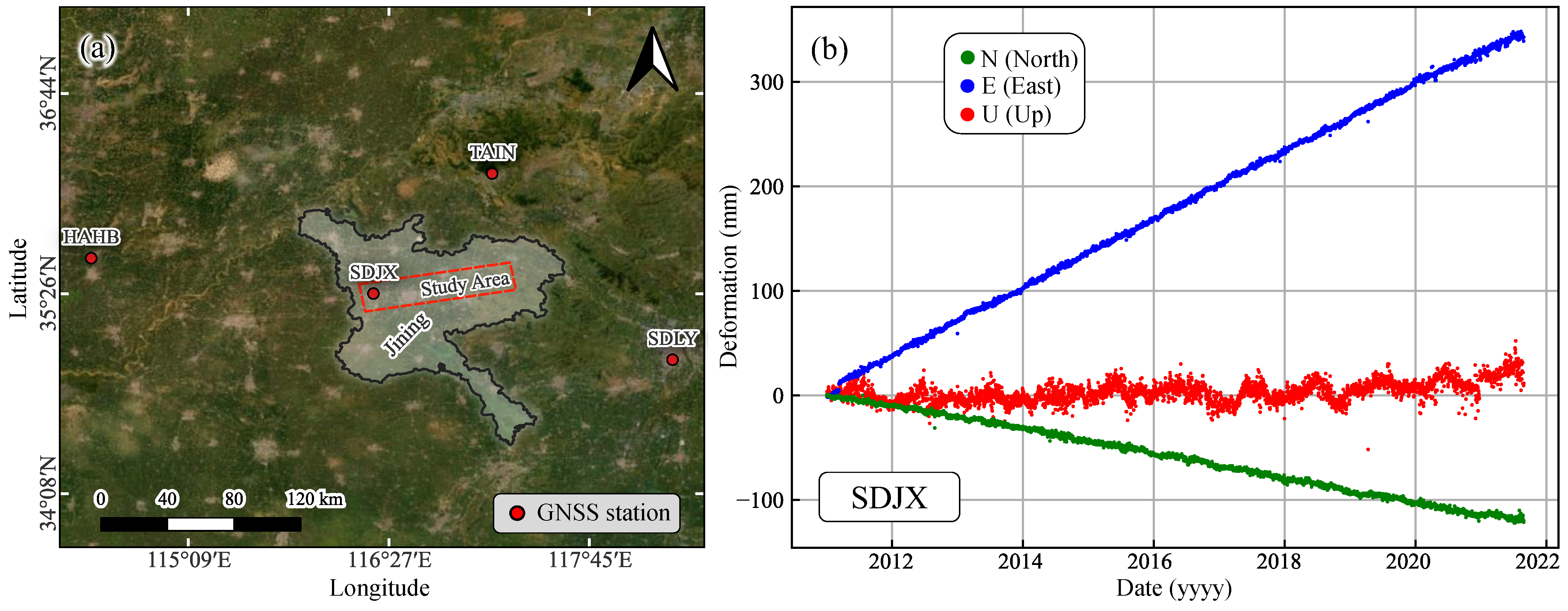
4.1. Data and Processing

To demonstrate the advantages of the SSBAS-InSAR method, we selected the Jining region in China as the study area for experiments and comparisons with the conventional SBAS-InSAR method. The selected area is depicted in Figure 4. Jining is a typical plain region with an elevation primarily between 50 and 100 m. As shown in Figure 4b, the land cover is mainly farmland and buildings. Frequent coal mining activities in Jining result in widespread surface subsidence.
We selected 125 scenes of SAR data obtained by the Sentinel-1 satellite from 3 December 2016 to 24 March 2021. The dates of the selected data are shown in Table A1 in Appendix A. The selected data are derived from a single burst in the Sentinel-1 satellite Interferometric Wide (IW) swath mode, with a coverage area of approximately 85 × 20 km and a spatial resolution of 5 × 20 m. The selected burst ID is 142_303065_IW2. The Sentinel-1 satellite has a single-satellite revisit period of 12 days and is equipped with a C-band synthetic aperture radar with a signal wavelength of 5.6 cm. The DEM data use the Copernicus 30-m resolution DEM (GLO-30), and the orbit data use the POD Precise Orbit Ephemerides.
Given the extensive cultivated lands in the study area, which are prone to temporal decorrelation, only three temporally adjacent images were selected for pairwise combination. The spatial baseline threshold was set to 200 m. The spatiotemporal baseline connection diagram is shown in Figure 5. Data preprocessing was performed using ISCE [37] with a multi-look parameter of 5 × 1 (range × azimuth). Phase filtering was conducted using the Goldstein method with a filter strength of 0.5. The phase unwrapping was completed using SNAPHU, and the final unwrapping result was geocoded at a resolution of 20 m.
The reference point was selected within the urban area of Jining City. Stacking-InSAR processing was then performed, and the average coherence of all interferometric pairs was calculated. The processing results are shown in Figure 6.
Areas with an average coherence below 0.8 were masked, and relatively stable points were then selected based on the masked Stacking-InSAR deformation rate results. The primary deformation in this area is surface subsidence caused by mining, with a deformation scale typically not exceeding 5 km. From the Stacking-InSAR processing results in Figure 6a, it is evident that there is no significant large-scale deformation in this region. For this experiment, the spatial scale of the SSBAS-InSAR method was set to 5 km, meaning high-coherence stable points were evenly selected at approximately 5 km intervals. Due to limitations such as coherence and the distribution of deformation areas, the actual distribution of selected points, shown in Figure 7, consists of 45 points in total. It is noteworthy that even after masking areas with an average coherence below 0.8, the maximum deformation rate in the Stacking-InSAR results still reached 12.95 cm/year, indicating that areas with significant deformation can still maintain high coherence. This finding suggests that selecting control points solely based on high coherence may not be entirely reliable.
Based on the selected control points and using Equation (12), the unwrapping images are corrected. On a laptop equipped with an Intel i7-1165G7 processor, the average time for single-threaded correction of each image is 3.7 s. This indicates that the proposed method does not impose a significant computational burden, and the phase correction process is efficient. As can be seen from Figure 8, after being constrained by multiple control points, the long-wavelength signal in the unwrapping images is weakened. There is a large area of arable land in Jining. The interference coherence in summer is low, and the phase unwrapping error is more serious than in winter. There are very obvious long-wavelength signals in Figure 8j,m,p. The absolute value of the maximum phase correction of some unwrapped data has exceeded 20 rad, as shown in Figure 8l. The converted deformation deviation exceeds 9 cm, which will have a significant impact on subsequent time-series processing. In Figure 8l,o, noticeable non-smooth-phase variations in the spatial domain are observed. This occurs because the phase correction is performed independently for each sub-triangle within the Delaunay triangulation using inverse distance weighting. When the original phase data contain significant errors with abrupt spatial variations, it may lead to large discrepancies in phase correction between different sub-triangles within the Delaunay network.
Figure 9 shows the deformation rates obtained by time-series processing using the conventional SBAS-InSAR method and the SSBAS-InSAR method. The reference points selected by the conventional SBAS-InSAR method are consistent with the reference points of the Stacking-InSAR method in Figure 6. The time-series processing steps are all completed by the weighted least squares method [21] of MintPy. The deformation rate results obtained from the SBAS-InSAR method and the SSBAS-InSAR method do not show significant differences. This is primarily due to both methods utilizing a large amount of SAR imagery, which significantly reduces the impact of random errors on the deformation rate calculations.

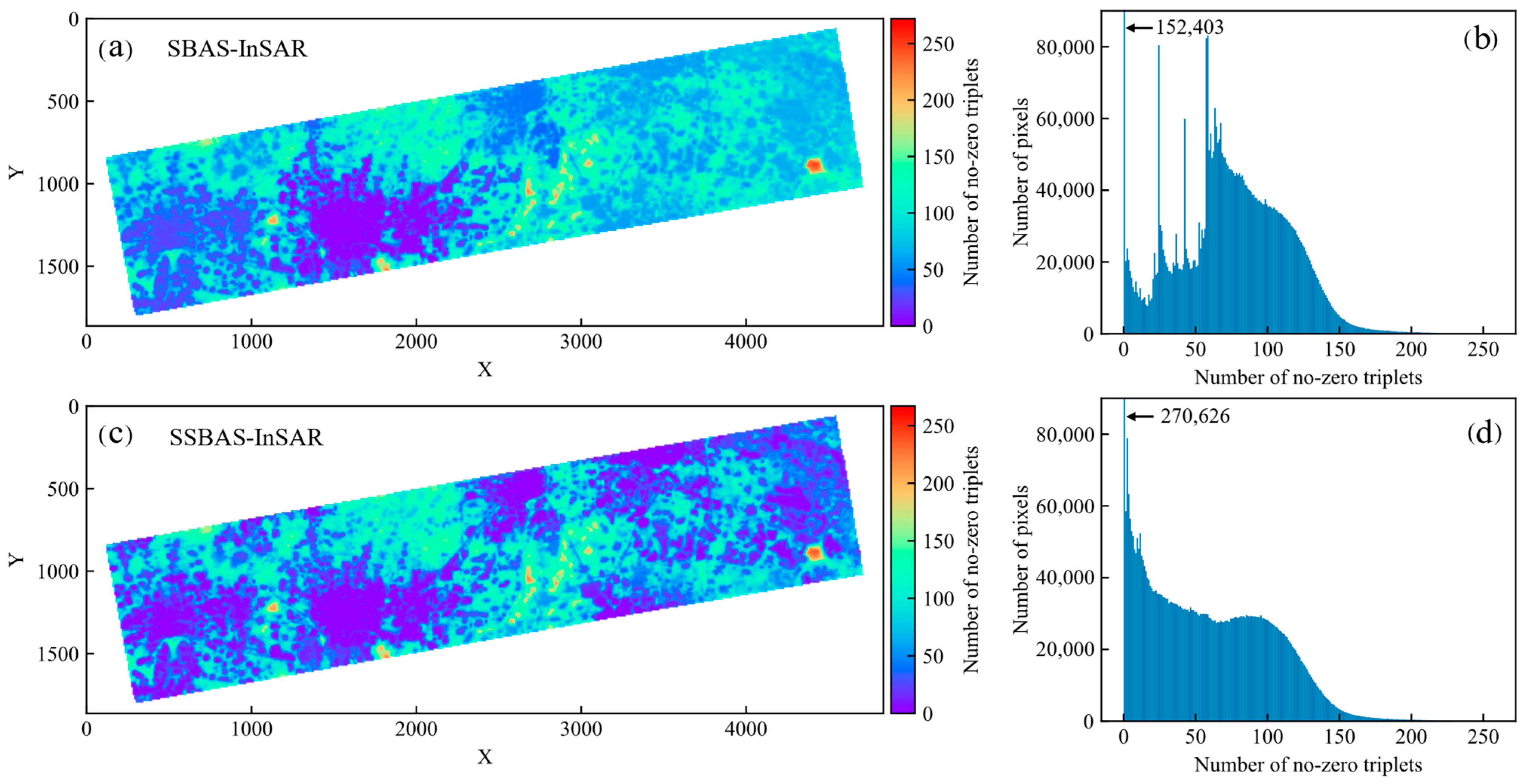
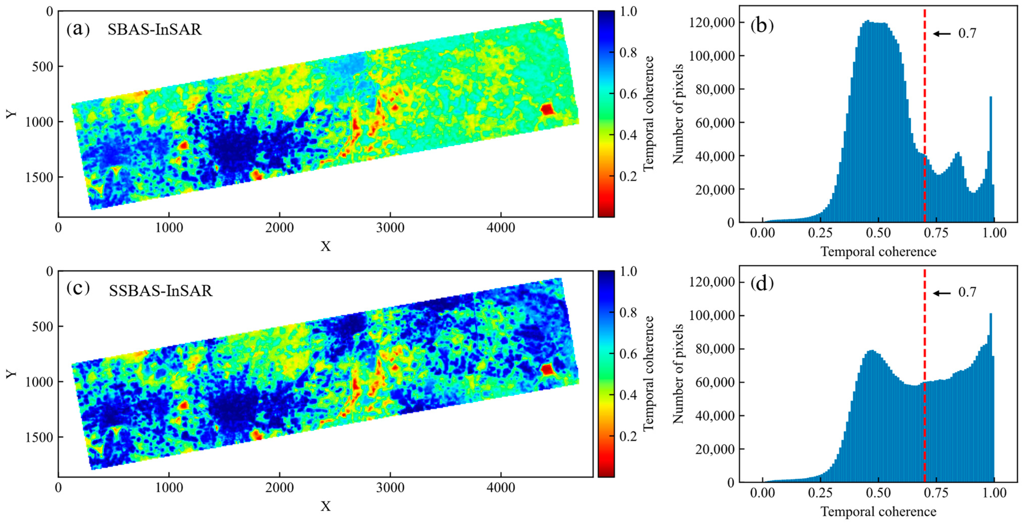
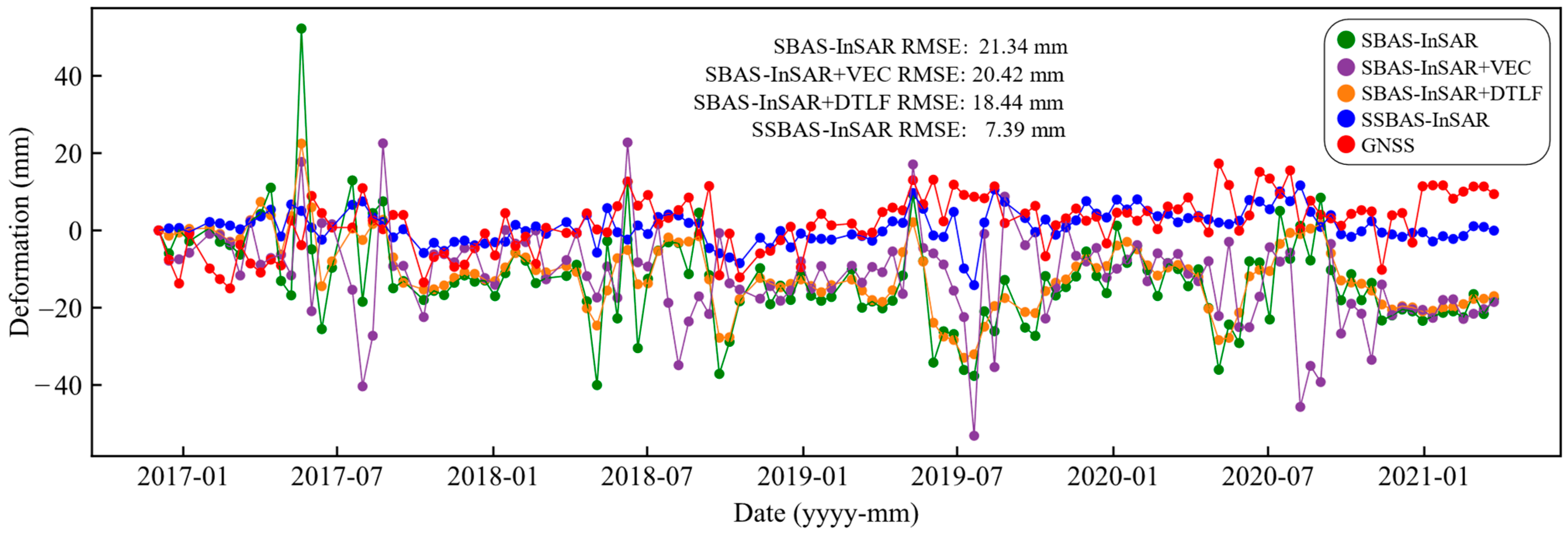
4.2. Precision Analysis

This study evaluates the performance of the conventional SBAS-InSAR method and the SSBAS-InSAR method across four dimensions: triangular phase closure, temporal coherence, standard deviation of deformation rate, and phase residue.
The calculation method for triangular phase closure is shown in Appendix B. A total of 367 triangular phase closure groups were formed based on the spatiotemporal baseline connection method given in Figure 5. Figure 10 displays the number of unreliable triangular phase closures per pixel, for both the conventional SBAS-InSAR method and the SSBAS-InSAR method. The results indicate that the triangular phase closure quality of the SSBAS-InSAR method is superior to that of the conventional SBAS-InSAR method. Combining the land cover types shown in Figure 4b and the average coherence in Figure 6a, it can be seen that the SSBAS-InSAR method consistently achieves higher triangular phase closure quality in high-coherence built areas. In contrast, the SBAS-InSAR method only achieves high triangular phase closure quality in certain portions of these built areas.
Temporal coherence is usually used to evaluate the quality of time-series data [21,39]. Here, we set the temporal coherence threshold to 0.7 to remove time-series data of poor quality. As can be seen from Figure 11, the temporal coherence obtained by the conventional SBAS-InSAR method is generally lower than that of the SSBAS-InSAR method. After removing the data with a temporal coherence lower than 0.7, the SBAS-InSAR method retains about 950,000 monitoring points, and the SSBAS-InSAR method retains about 2.09 million monitoring points.
When comparing the standard deviation of velocity [40] and phase residue [21], the SSBAS-InSAR method clearly outperforms the conventional SBAS-InSAR method, as shown in Figure 12 and Figure 13. The SSBAS-InSAR method consistently maintains a lower standard deviation of velocity and phase residue across the entire study area. This improvement is particularly noticeable in the right half of the study area, where both metrics are significantly reduced compared to the conventional SBAS-InSAR method.
The study area was divided into eight sub-areas to facilitate a comparative analysis of the phase residue within each sub-area. The division of the sub-areas is depicted in Figure 13, while the phase residue comparison for each patch is illustrated in Figure 14. The average phase residue values for each patch are summarized in Table 1. Across all eight sub-areas, the SSBAS-InSAR method consistently yields lower average phase residue compared to the conventional SBAS-InSAR method. Notably, because the reference point selected for the conventional SBAS-InSAR method is situated in patch 6, the average phase residue in this patch is similar between the two methods. However, in patches farther from patch 6, the conventional method exhibits a significantly higher average phase residue than the SSBAS-InSAR method.

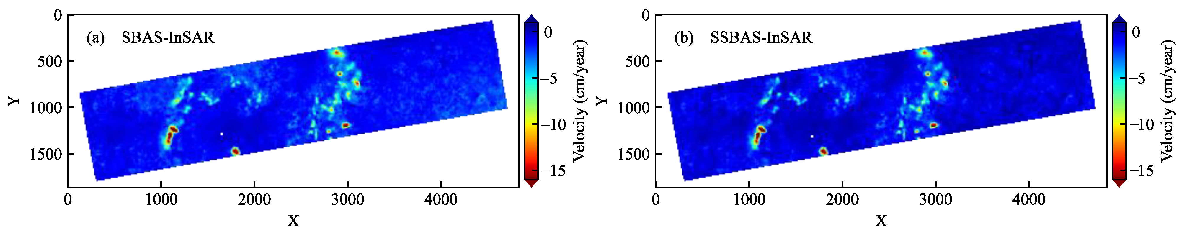
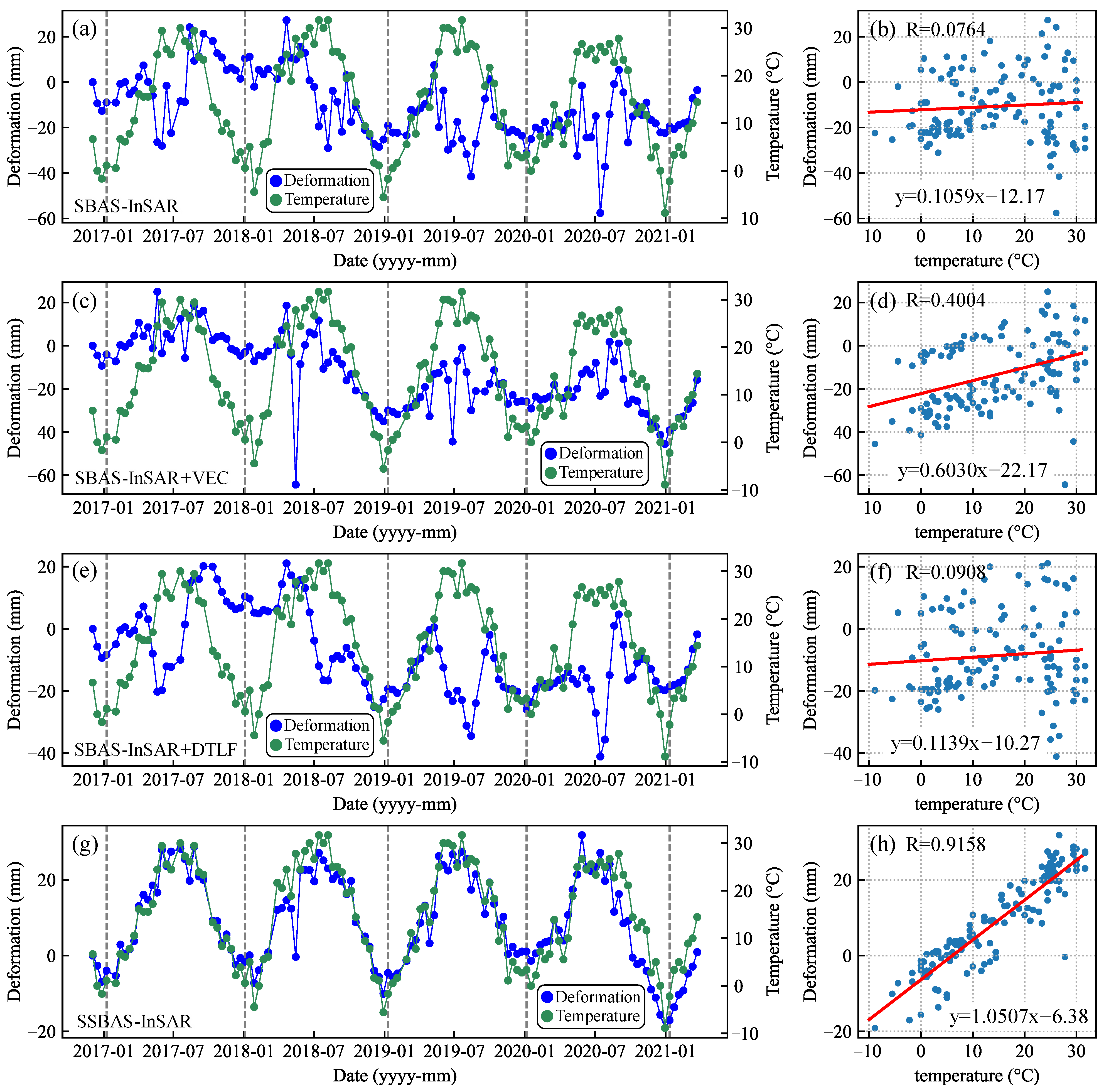
4.3. Comparative Analysis of Time-Series Deformation

Figure 15 shows the deformation rate results obtained by the SBAS-InSAR and SSBAS-InSAR methods after applying a temporal coherence threshold of 0.7. The conventional SBAS-InSAR method, which uses a single reference point, exhibits an insufficient error constraint capability, leading to almost complete masking of the area far from the reference point in the right half of the study area. In contrast, the SSBAS-InSAR method provides significantly better coverage of the deformation results.
In the time-series deformation comparison, we not only included the conventional SBAS-InSAR method and the SSBAS-InSAR method, but also introduced two additional methods: SBAS-InSAR with various error corrections (denoted as SBAS-InSAR+VEC) [21] and SBAS-InSAR with dual-scale temporal low-pass filtering (denoted as SBAS-InSAR+DTLF) [24]. Both of these additional methods involve subsequent processing based on the time-series results obtained from the conventional SBAS-InSAR method. The characteristics of these four methods are summarized in Table 2.
We compared the time-series deformation curves obtained using four different methods across various regions. Four specific points were selected for this comparison, as illustrated in Figure 15 and Figure 16. These points include: P1, located in a building area; P2, situated in a coal mining subsidence area; P3, positioned on a hillside; and SDJX, a GNSS (Global Navigation Satellite System) monitoring station.
In the time-series deformation curve of point P1, the SSBAS-InSAR method reveals a clear periodic pattern. According to the optical remote sensing image in Figure 16, point P1 is situated on the roof of a steel-structure building. Such buildings typically experience deformation due to temperature fluctuations. Over a temperature range of −20 °C to 60 °C, the deformation of steel structures is linearly related to temperature changes [41], as described by Equation (13).
Δ L = b L 0 Δ T
where Δ L is the deformation, b is the thermal expansion coefficient, L 0 is the length of the steel structure, and Δ T is the temperature change.
Based on the linear relationship between steel structure deformation and temperature, we calculated the correlation coefficient between the time-series deformation data for point P1 and temperature for all four methods. The surface temperature data, which consist of daily average temperatures, were obtained from NOAA (National Oceanic and Atmospheric Administration). The location of the temperature monitoring station is indicated by the “YANZHOU, CH” label in Figure 15.
The correlation coefficient between the deformation at point P1 and temperature, based on the SSBAS-InSAR method, is 0.9158. In contrast, the correlation coefficient based on the conventional SBAS-InSAR method is only 0.0764. Figure 17 illustrates the comparison between deformation and temperature results obtained by the four methods. The slope of the relationship between deformation and surface temperature at point P1, as determined by the SSBAS-InSAR method, is 1.0507 mm/°C.
Point P2 is situated in a coal mining subsidence area. Due to the typically nonlinear nature of surface time-series deformation curves in such areas, traditional linear models often yield substantial errors when used for fitting. The Logistic model, which represents a typical S-shaped curve, offers a more accurate depiction of surface deformation in mining regions, and has been extensively applied in related research [42,43]. The Logistic model is described by Equation (14). Analysis of the time-series deformation results obtained by the SSBAS-InSAR method at point P2 reveals two distinct subsidence stages throughout the monitoring period. We divided the time-series deformation curve for point P2 into three segments and applied the Logistic model, linear model, and Logistic model sequentially, as illustrated in Figure 18.
After segmenting and fitting the data, the root mean square error (RMSE) between the observed deformation values and the fitted values across all time points was calculated. The RMSE of the conventional SBAS-InSAR method is the highest, at 8.68 mm, while the RMSE of the SSBAS-InSAR method is 3.96 mm.
W ( t ) = W 0 1 + c 1 e c 2 t
where W ( t ) is the deformation at time t , W 0 is the maximum deformation, and c 1 and c 2 are constants.
Point P3 is situated on a hillside with the slope oriented towards the SAR satellite, as shown in Figure 19a. According to Figure 15, the conventional SBAS-InSAR method’s deformation results at this location are masked due to low temporal coherence. To analyze the deformation curves obtained by all four methods at point P3, we extracted the SBAS-InSAR time-series results for point P3 before applying the temporal coherence threshold mask and compared them with the time-series results from the SSBAS-InSAR method, as depicted in Figure 19b. The temporal coherence at point P3 is 0.631 for the conventional SBAS-InSAR method and 0.962 for the SSBAS-InSAR method. Comparing the time-series deformation curves reveals that the SBAS-InSAR method exhibits significant random fluctuations, with more pronounced variations during the summer, which obscure the deformation trend at point P3. Similarly, the deformation curves obtained by the SBAS-VEC and SBAS-DTLF methods also show prominent fluctuations. In contrast, the deformation curve from the SSBAS-InSAR method shows a clear linear trend, indicating movement towards the SAR satellite. Based on the slope aspect information, it is inferred that the area where point P3 is located is likely experiencing a downslope sliding trend.
SDJX is one of the GNSS stations of CMONOC (Crustal Movement Observation Network of China), with its monitoring data processed using GAMIT. These GNSS results are considered as true values for comparing the monitoring effects of the SBAS-InSAR and SSBAS-InSAR methods in this area. Since the deformation direction obtained from InSAR is aligned with the line of sight of the SAR satellite, the GNSS deformation data must first be converted to the line of sight of the SAR satellite. The conversion formula is provided in Equation (15).
G N S S l o s = sin θ sin α G N S S n sin θ cos α G N S S e + cos θ G N S S u
Here, G N S S l o s represents the deformation value in the SAR satellite line of sight direction; G N S S n , G N S S e and G N S S u represent the deformation values in the north, east, and vertical directions, respectively; θ is the SAR satellite incident angle, and α is the SAR satellite azimuth angle (starting from the north direction and calculated clockwise).
According to previous studies, the Chinese mainland plate exhibits a noticeable eastward movement [44], and the SDJX station also shows significant horizontal movement, as illustrated in Figure 20. Furthermore, multiple GNSS stations located hundreds of kilometers away from SDJX display horizontal movement with the same trend and magnitude, as detailed in Table 3. However, the InSAR processing results provide only relative deformation within the study area, and do not capture the overall trend of plate displacement [45]. To mitigate the influence of horizontal movement on the comparison between InSAR and GNSS results, the horizontal movement is disregarded when converting GNSS deformation results to the SAR satellite line of sight, focusing solely on vertical deformation.
As depicted in Figure 21, the deformation curve obtained from the SSBAS-InSAR method is relatively stable and closely matches the GNSS results, while the deformation curves obtained by the other three methods show significant random fluctuations. At point SDJX, the RMSE of the SBAS-InSAR method has the highest RMSE, at 21.34 mm, while the RMSE of the SSBAS-InSAR method is 7.39 mm.

5. Discussion

5.1. Reliability of the SSBAS-InSAR Method

In the study area of Jining, China, we compared the results of the SBAS-InSAR and SSBAS-InSAR methods. The SSBAS-InSAR method demonstrates superior performance over the conventional SBAS-InSAR method in terms of triangular phase closure, temporal coherence, deformation rate standard deviation, and phase residue, as shown in Figure 10, Figure 11, Figure 12 and Figure 13. Particularly in areas distant from the SBAS-InSAR reference point, specifically on the right side of the study area, the conventional SBAS-InSAR method shows significantly reduced monitoring accuracy compared to the SSBAS-InSAR method. After applying a temporal coherence threshold of 0.7, the SBAS-InSAR method retains approximately 950,000 monitoring points, while the SSBAS-InSAR method retains about 2.09 million monitoring points. Consequently, the SSBAS-InSAR method maintains roughly twice as many monitoring points as the conventional SBAS-InSAR method, as illustrated in Figure 11 and Figure 15.
In the analysis of time-series deformation curves in various typical deformation areas, the SSBAS-InSAR method demonstrates strong monitoring performance. At point P1, located on a steel-structured building, the deformation curve from the SSBAS-InSAR method shows a high correlation with temperature, with a correlation coefficient of 0.9158. In contrast, the correlation coefficients of the other three methods are much lower, as illustrated in Figure 17. For point P2, situated in a mining area, the deformation curve from the SSBAS-InSAR method aligns well with the Logistic model, yielding an RMSE of only 3.96 mm before and after fitting, as shown in Figure 18. At point P3 on a hillside, the deformation curve from the SSBAS-InSAR method reveals a clear linear trend towards the satellite direction, as demonstrated in Figure 19. Compared to the GNSS results at the SDJX point, the SSBAS-InSAR method achieves an RMSE of 7.39 mm, which is significantly better than the other three methods, as shown in Figure 21.
Compared to the SBAS-InSAR, SBAS-InSAR+VEC, and SBAS-InSAR+DTLF methods, the SSBAS-InSAR method has demonstrated superior performance in monitoring various types of deformation. It effectively captures temperature-related deformation in steel-structured buildings, surface subsidence in mining areas, and slip trends on hillsides. The SSBAS-InSAR method provides a clearer depiction of local deformation information, indicating its ability to enhance the accuracy and reliability of deformation monitoring over extensive areas.

5.2. Characteristics of the SSBAS-InSAR Method

Due to the computational simplicity of the Stacking-InSAR method, which efficiently captures surface deformation distributions, the SSBAS-InSAR method utilizes its results as prior information to identify stable regions. The deformation rates of the control points selected from these stable regions were all set to zero. This approach leads to a partial attenuation of long-wavelength deformation information. Similar to how elevation-related atmospheric phase corrections may inaccurately adjust elevation-related deformations, and linear functions may inadvertently remove long-wavelength deformation signals while correcting residual orbit phase ramps [21], or how spatial domain low-pass filtering may also suppress long-wavelength deformation signals while addressing atmospheric turbulence [46], the proposed method exhibits certain limitations.
Our method focuses on small spatial-scale deformations across extensive surfaces, making it particularly effective for monitoring phenomena such as mining subsidence, landslides, and other small-scale deformations. Such monitoring requires attention to finer local changes, thereby minimizing the impact of long-wavelength signals (including long-wavelength deformation and error signals) and enhancing the representation of local deformation information. Theoretically, a higher density of control points results in smaller spatial-dimension error propagation and improved deformation monitoring accuracy. However, the density of control points cannot increase indefinitely, as it is influenced by the spatial scale of the deformation being monitored. For different types of deformation monitoring, it is essential to consider the deformation characteristics to determine a reasonable control point density. An excessively high density of control points may lead to incorrect deformation corrections, while a too-low density may result in insufficient error constraint capability. Unlike methods such as LiCSBAS [22], the SSBAS-InSAR method does not apply spatiotemporal filtering to its results, thus preserving a greater amount of deformation detail. Despite the lack of time-domain filtering, the SSBAS-InSAR method can still produce relatively smooth time-series deformation curves, a benefit attributed to the spatial-scale constraints inherent in the SSBAS-InSAR approach.
Since June 2023, the Alaska Satellite Facility (ASF) has begun providing Sentinel-1 single burst data products to address the challenges associated with Sentinel-1 SLC data offsets and the large size of single SLC files [47]. In the future, InSAR processing using Sentinel-1 single burst data is likely to become a mainstream choice for users. However, single-burst data consist of narrow strips where the spatial length in the range direction is approximately four times that in the azimuth direction. This disparity increases the difficulty of phase unwrapping, particularly in low-coherence regions, where it may result in more severe error propagation. In the experiment conducted in Jining, China, the SSBAS-InSAR method demonstrates a significant advantage in processing single-burst data.

6. Conclusions

This paper explores the spatial characteristics of various factors affecting phase unwrapped data, including atmospheric phase errors, orbit errors, and phase unwrapping errors. The relationship between the phase error and the spatial scale is discussed, demonstrating that constraining the spatial scale can mitigate phase errors. Building on this insight, a novel SSBAS-InSAR method is introduced that leverages spatial constraints. This method involves selecting ground points with high coherence and stability based on Stacking-InSAR processing results and employing multiple ground control points to create a Delaunay triangulation network. This network helps to constrain error propagation in the spatial dimension. Compared to the conventional SBAS-InSAR method, the proposed approach yields monitoring results with higher accuracy and increased point density.
The SSBAS-InSAR method has the following characteristics:
(1).
The concept of spatial scale is introduced to constrain the transmission of errors in the spatial dimension, thereby improving the accuracy of deformation monitoring;
(2).
The control points are selected by combining the Stacking-InSAR results with the average coherence, which improves the reliability of the control point selection;
(3).
The phase is corrected by inverse distance weighting only based on the Delaunay triangulation, without applying any other spatiotemporal filtering methods, which retains the time-series deformation details.
The method proposed in this paper is suitable for the fine-grained deformation monitoring of wide-area surfaces, such as the fine-grained monitoring of deformation types such as landslides and mining subsidence on wide-area surfaces. When the research object is large-scale deformation, the applicability of the method proposed in this paper should be carefully considered.
The SSBAS-InSAR method is implemented on the basis of the conventional SBAS-InSAR method. Some processing procedures are consistent with the processing procedures of the conventional SBAS-InSAR method. With the help of existing open-source time-series InSAR processing software, such as MintPy and GMTSAR, the processing procedures of the SSBAS-InSAR method can be quickly implemented.

Author Contributions

Conceptualization, Z.Y. and G.Z.; methodology, Z.Y.; software, G.Z.; validation, G.H., C.C. and Z.Z.; formal analysis, C.Z.; investigation, Z.Y.; resources, G.Z.; data curation, Z.Y. and G.Z.; writing—original draft preparation, Z.Y.; writing—review and editing, Z.Y., G.Z. and G.H. All authors have read and agreed to the published version of the manuscript.

Funding

This research was funded by the National Key R&D Program of China, grant number 2022YFB3902601, and the National Natural Science Foundation of China (NSFC), grant number 52278359.

Data Availability Statement

The Sentinel-1 data used in this research can be downloaded from the ASF (Alaska Satellite Facility) website (https://search.asf.alaska.edu/ (accessed on 19 June 2024)), and the temperature data can be downloaded from the NOAA (National Oceanic and Atmospheric Administration) website (https://www.ncei.noaa.gov/maps/daily/ (accessed on 19 June 2024)).

Acknowledgments

The authors gratefully acknowledges the Sentinel-1 data provided by ESA (European Space Agency). The data processing was conducted using the ISCE (https://github.com/isce-framework/isce2, accessed on 19 June 2024) and MintPy (https://github.com/insarlab/MintPy, accessed on 19 June 2024) software, and the paper’s plots were produced using QGIS (https://qgis.org/en/site/, accessed on 19 June 2024) and matplotlib (https://matplotlib.org/, accessed on 19 June 2024). We thank the three anonymous reviewers for their insightful comments and suggestions.

Conflicts of Interest

The authors declare no conflicts of interest.

Appendix A

Table A1. SAR imagery date list. The date format is yyyymmdd.
No.DateNo.DateNo.DateNo.DateNo.DateNo.Date
120161203222017090543201806086420190311852019113010620200808
220161215232017091744201806206520190323862019121210720200820
320161227242017101145201807026620190404872019122410820200901
420170108252017102346201807146720190416882020010510920200913
520170201262017110447201807266820190428892020011711020200925
620170213272017111648201808076920190510902020012911120201007
720170225282017112849201808197020190522912020021011220201019
820170309292017121050201808317120190603922020022211320201031
920170321302017122251201809127220190615932020030511420201112
1020170402312018010352201809247320190627942020031711520201124
1120170414322018011553201810067420190709952020032911620201206
1220170426332018012754201810187520190721962020041011720201218
1320170508342018020855201811117620190802972020042211820201230
1420170520352018022056201811237720190814982020050411920210111
1520170601362018030457201812057820190826992020051612020210123
16201706133720180328582018121779201909191002020052812120210204
17201706253820180409592018122980201910011012020060912220210216
18201707193920180421602019011081201910131022020062112320210228
19201707314020180503612019012282201910251032020070312420210312
20201708124120180515622019020383201911061042020071512520210324
212017082442201805276320190227842019111810520200727

Appendix B

In triangular phase closure, with three images a, b, and c taken in sequence, the sum of the interferometric unwrapped phases from images a to b and from b to c should theoretically equal the interferometric unwrapped phase from a to c [48]. The schematic diagram of triangular phase closure is illustrated in Figure 10. Due to phase noise and processing operations such as multi-looking and spatial filtering, the triangular phase closure may not be perfectly achieved even in the absence of phase unwrapping errors. The absolute value of the triangular phase closure error is given by Equation (A1), and the number of unreliable triangular phase closure groups is defined by Equation (A2).
Figure A1. Schematic diagram of triangle phase closure.
Remotesensing 16 03515 g0a1
C d i f f = | C a b + C b c C a c |
where C d i f f is the absolute value of the phase closure error; C a b , C b c and C a c represent the interferometric unwrapped phase values between a , b and c images.
C s u m = k N { 0 1       C ( d i f f , k ) < π       C ( d i f f , k ) π
where C s u m is the number of unreliable phase closures, N is the number of phase closure groups, and C ( d i f f , k ) is the absolute value of the phase closure difference of the phase closure group. Using π rad as the threshold, the number of triangular phase closure groups with absolute closure errors greater than or equal to π rad is counted.

References

  1. Yang, Z.; Li, Z.; Zhu, J.; Wang, Y.; Wu, L. Use of SAR/InSAR in Mining Deformation Monitoring, Parameter Inversion, and Forward Predictions: A Review. IEEE Geosci. Remote Sens. Mag. 2020, 8, 71–90. [Google Scholar] [CrossRef]
  2. He, K.; Lombardo, L.; Chang, L.; Sadhasivam, N.; Hu, X.; Fang, Z.; Dahal, A.; Fadel, I.; Luo, G.; Tanyas, H. Investigating Earthquake Legacy Effect on Hillslope Deformation Using InSAR-Derived Time Series. Earth Surf. Proc. Landf. 2024, 49, 980–990. [Google Scholar] [CrossRef]
  3. Xu, X.; Sandwell, D.T.; Smith-Konter, B. Coseismic Displacements and Surface Fractures from Sentinel-1 InSAR: 2019 Ridgecrest Earthquakes. Seismol. Res. Lett. 2020, 91, 1979–1985. [Google Scholar] [CrossRef]
  4. D’Amico, F.; Gagliardi, V.; Bianchini Ciampoli, L.; Tosti, F. Integration of InSAR and GPR Techniques for Monitoring Transition Areas in Railway Bridges. NDT E Int. 2020, 115, 102291. [Google Scholar] [CrossRef]
  5. Osmanoğlu, B.; Sunar, F.; Wdowinski, S.; Cabral-Cano, E. Time Series Analysis of InSAR Data: Methods and Trends. Isprs J. Photogramm. Remote Sens. 2016, 115, 90–102. [Google Scholar] [CrossRef]
  6. Aswathi, J.; Binoj Kumar, R.B.; Oommen, T.; Bouali, E.H.; Sajinkumar, K.S. InSAR as a Tool for Monitoring Hydropower Projects: A Review. Energy Geosci. 2022, 3, 160–171. [Google Scholar] [CrossRef]
  7. Li, S.; Xu, W.; Li, Z. Review of the SBAS InSAR Time-Series Algorithms, Applications, and Challenges. Geod. Geodyn. 2022, 13, 114–126. [Google Scholar] [CrossRef]
  8. Wu, Y.-Y.; Madson, A. Error Sources of Interferometric Synthetic Aperture Radar Satellites. Remote Sens. 2024, 16, 354. [Google Scholar] [CrossRef]
  9. Kirui, P.K.; Reinosch, E.; Isya, N.; Riedel, B.; Gerke, M. Mitigation of Atmospheric Artefacts in Multi Temporal InSAR: A Review. PFG–J. Photogramm. Remote Sens. Geoinf. Sci. 2021, 89, 251–272. [Google Scholar] [CrossRef]
  10. Li, Z.; Duan, M.; Cao, Y.; Mu, M.; He, X.; Wei, J. Mitigation of Time-Series InSAR Turbulent Atmospheric Phase Noise: A Review. Geod. Geodyn. 2022, 13, 93–103. [Google Scholar] [CrossRef]
  11. Liang, H.; Zhang, L.; Lu, Z.; Li, X. Correction of Spatially Varying Stratified Atmospheric Delays in Multitemporal InSAR. Remote Sens. Environ. 2023, 285, 113382. [Google Scholar] [CrossRef]
  12. Yu, Z.; Huang, G.; Zhao, Z.; Huang, Y.; Zhang, C.; Zhang, G. A Multi-Scale Spatial Difference Approach to Estimating Topography Correlated Atmospheric Delay in Radar Interferograms. Remote Sens. 2023, 15, 2115. [Google Scholar] [CrossRef]
  13. Yu, C.; Li, Z.; Penna, N.T.; Crippa, P. Generic Atmospheric Correction Model for Interferometric Synthetic Aperture Radar Observations. J. Geophys. Res. Solid Earth 2018, 123, 9202–9222. [Google Scholar] [CrossRef]
  14. Yu, C.; Penna, N.T.; Li, Z. Generation of Real-time Mode High-resolution Water Vapor Fields from GPS Observations. J. Geophys. Res. Atmos. 2017, 122, 2008–2025. [Google Scholar] [CrossRef]
  15. Yu, C.; Li, Z.; Penna, N.T. Interferometric Synthetic Aperture Radar Atmospheric Correction Using a GPS-Based Iterative Tropospheric Decomposition Model. Remote Sens. Environ. 2018, 204, 109–121. [Google Scholar] [CrossRef]
  16. Hanssen, R.F. Radar Interferometry: Data Interpretation and Error Analysis; Remote Sensing and Digital Image Processing; Kluwer Academic Publishers: Dordrecht, The Netherlands, 2010; ISBN 978-0-306-47633-4. [Google Scholar]
  17. Liu, G.; Hanssen, R.F.; Guo, H.; Yue, H.; Perski, Z. Nonlinear Model for InSAR Baseline Error. IEEE Trans. Geosci. Remote Sensing 2016, 54, 5341–5351. [Google Scholar] [CrossRef]
  18. Du, Y.; Fu, H.; Liu, L.; Feng, G.; Peng, X.; Wen, D. Orbit Error Removal in InSAR/MTInSAR with a Patch-Based Polynomial Model. Int. J. Appl. Earth Obs. Geoinf. 2021, 102, 102438. [Google Scholar] [CrossRef]
  19. Wang, S.; Zhang, G.; Chen, Z.; Cui, H.; Zheng, Y.; Xu, Z.; Li, Q. Surface Deformation Extraction from Small Baseline Subset Synthetic Aperture Radar Interferometry (SBAS-InSAR) Using Coherence-Optimized Baseline Combinations. GIScience Remote Sens. 2022, 59, 295–309. [Google Scholar] [CrossRef]
  20. Zhang, Z.; Li, J.; Duan, P.; Chang, J. Creep Identification by the Baseline Optimized TS-InSAR Technique Considering the Monthly Variation in Coherence. Geocarto Int. 2022, 38, 2159071. [Google Scholar] [CrossRef]
  21. Yunjun, Z.; Fattahi, H.; Amelung, F. Small Baseline InSAR Time Series Analysis: Unwrapping Error Correction and Noise Reduction. Comput. Geosci. 2019, 133, 104331. [Google Scholar] [CrossRef]
  22. Morishita, Y.; Lazecky, M.; Wright, T.; Weiss, J.; Elliott, J.; Hooper, A. LiCSBAS: An Open-Source InSAR Time Series Analysis Package Integrated with the LiCSAR Automated Sentinel-1 InSAR Processor. Remote Sens. 2020, 12, 424. [Google Scholar] [CrossRef]
  23. Oliver-Cabrera, T.; Jones, C.E.; Yunjun, Z.; Simard, M. InSAR Phase Unwrapping Error Correction for Rapid Repeat Measurements of Water Level Change in Wetlands. IEEE Trans. Geosci. Remote Sens. 2022, 60, 5215115. [Google Scholar] [CrossRef]
  24. Wu, H.; Zhang, Y.; Kang, Y.; Wei, J.; Lu, Z.; Yan, W.; Wang, H.; Liu, Z.; Lv, X.; Zhou, M.; et al. SAR Interferometry on Full Scatterers: Mapping Ground Deformation with Ultra-High Density from Space. Remote Sens. Environ. 2024, 302, 113965. [Google Scholar] [CrossRef]
  25. Bekaert, D.P.S.; Handwerger, A.L.; Agram, P.; Kirschbaum, D.B. InSAR-Based Detection Method for Mapping and Monitoring Slow-Moving Landslides in Remote Regions with Steep and Mountainous Terrain: An Application to Nepal. Remote Sens. Environ. 2020, 249, 111983. [Google Scholar] [CrossRef]
  26. Kang, Y.; Lu, Z.; Zhao, C.; Xu, Y.; Kim, J.; Gallegos, A.J. InSAR Monitoring of Creeping Landslides in Mountainous Regions: A Case Study in Eldorado National Forest, California. Remote Sens. Environ. 2021, 258, 112400. [Google Scholar] [CrossRef]
  27. Cao, Y.; Li, Z.; Amelung, F. Mapping Ground Displacement by a Multiple Phase Difference-Based InSAR Approach: With Stochastic Model Estimation and Turbulent Troposphere Mitigation. J. Geod. 2019, 93, 1313–1333. [Google Scholar] [CrossRef]
  28. Zebker, H. Accuracy of a Model-Free Algorithm for Temporal InSAR Tropospheric Correction. Remote Sens. 2021, 13, 409. [Google Scholar] [CrossRef]
  29. Zhang, B.; Hestir, E.; Yunjun, Z.; Reiter, M.E.; Viers, J.H.; Schaffer-Smith, D.; Sesser, K.; Oliver-Cabrera, T. Automated Reference Points Selection for InSAR Time Series Analysis on Segmented Wetlands. IEEE Geosci. Remote Sens. Lett. 2024, 21, 4008705. [Google Scholar] [CrossRef]
  30. Wang, Y.; Feng, G.; Li, Z.; Luo, S.; Wang, H.; Xiong, Z.; Zhu, J.; Hu, J. A Strategy for Variable-Scale InSAR Deformation Monitoring in a Wide Area: A Case Study in the Turpan–Hami Basin, China. Remote Sens. 2022, 14, 3832. [Google Scholar] [CrossRef]
  31. Li, Z.W.; Ding, X.L.; Huang, C.; Zou, Z.R.; Chen, Y.L. Atmospheric Effects on Repeat-Pass InSAR Measurements over Shanghai Region. J. Atmos. Sol. Terr. Phys. 2007, 69, 1344–1356. [Google Scholar] [CrossRef]
  32. Fattahi, H.; Simons, M.; Agram, P. InSAR Time-Series Estimation of the Ionospheric Phase Delay: An Extension of the Split Range-Spectrum Technique. IEEE Trans. Geosci. Remote Sens. 2017, 55, 5984–5996. [Google Scholar] [CrossRef]
  33. Liang, C.; Agram, P.; Simons, M.; Fielding, E.J. Ionospheric Correction of InSAR Time Series Analysis of C-Band Sentinel-1 TOPS Data. IEEE Trans. Geosci. Remote Sens. 2019, 57, 6755–6773. [Google Scholar] [CrossRef]
  34. Uuemaa, E.; Ahi, S.; Montibeller, B.; Muru, M.; Kmoch, A. Vertical Accuracy of Freely Available Global Digital Elevation Models (ASTER, AW3D30, MERIT, TanDEM-X, SRTM, and NASADEM). Remote Sens. 2020, 12, 3482. [Google Scholar] [CrossRef]
  35. Chen, C.W.; Zebker, H.A. Two-Dimensional Phase Unwrapping with Use of Statistical Models for Cost Functions in Nonlinear Optimization. J. Opt. Soc. Am. A 2001, 18, 338. [Google Scholar] [CrossRef]
  36. Karra, K.; Kontgis, C.; Statman-Weil, Z.; Mazzariello, J.C.; Mathis, M.; Brumby, S.P. Global Land Use / Land Cover with Sentinel 2 and Deep Learning. In Proceedings of the 2021 IEEE International Geoscience and Remote Sensing Symposium IGARSS, Brussels, Belgium, 11 July 2021; IEEE: Piscataway, NJ, USA, 2021; pp. 4704–4707. [Google Scholar]
  37. Fattahi, H.; Agram, P.; Simons, M. A Network-Based Enhanced Spectral Diversity Approach for TOPS Time-Series Analysis. IEEE Trans. Geosci. Remote Sens. 2017, 55, 777–786. [Google Scholar] [CrossRef]
  38. Geudtner, D.; Miranda, N.; Navas-Traver, I.; Ceba, F.V.; Prats, P.; Yague-Martinez, N.; Breit, H.; de Zan, F.; Larsen, Y.; Recchia, A.; et al. Sentinel-1A/B SAR and InSAR Performance. In Proceedings of the EUSAR 2018; 12th European Conference on Synthetic Aperture Radar, Aachen, Germany, 4–7 June 2018. [Google Scholar]
  39. Pepe, A.; Lanari, R. On the Extension of the Minimum Cost Flow Algorithm for Phase Unwrapping of Multitemporal Differential SAR Interferograms. IEEE Trans. Geosci. Remote Sens. 2006, 44, 2374–2383. [Google Scholar] [CrossRef]
  40. Fattahi, H.; Amelung, F. InSAR Bias and Uncertainty Due to the Systematic and Stochastic Tropospheric Delay. J. Geophys. Res. Solid Earth 2015, 120, 8758–8773. [Google Scholar] [CrossRef]
  41. Han, Q.; Ma, Q.; Xu, J.; Liu, M. Structural Health Monitoring Research under Varying Temperature Condition: A Review. J. Civ. Struct. Health Monit. 2021, 11, 149–173. [Google Scholar] [CrossRef]
  42. Ma, P.; Yu, C.; Wu, Z.; Wang, Z.; Chen, J. Mining-Related Subsidence Measurements Using a Robust Multi-Temporal InSAR Method and Logistic Model. IEEE J. Miniaturiz. Air Space Syst. 2024, 5, 149–155. [Google Scholar] [CrossRef]
  43. Dai, S.; Zhang, Z.; Li, Z.; Liu, X.; Chen, Q. Prediction of Mining-Induced 3-D Deformation by Integrating Single-Orbit SBAS-InSAR, GNSS, and Log-Logistic Model (LL-SIG). IEEE Trans. Geosci. Remote Sens. 2023, 61, 5222213. [Google Scholar] [CrossRef]
  44. Wang, M.; Shen, Z. Present-day Crustal Deformation of Continental China Derived from GPS and Its Tectonic Implications. J. Geophys. Res. Solid Earth 2020, 125, e2019JB018774. [Google Scholar] [CrossRef]
  45. Stephenson, O.L.; Liu, Y.-K.; Yunjun, Z.; Simons, M.; Rosen, P.; Xu, X. The Impact of Plate Motions on Long-Wavelength InSAR-Derived Velocity Fields. Geophys. Res. Lett. 2022, 49, e2022GL099835. [Google Scholar] [CrossRef]
  46. Zhang, G.; Xu, Z.; Chen, Z.; Wang, S.; Liu, Y.; Gong, X. Analyzing Surface Deformation throughout China’s Territory Using Multi-Temporal InSAR Processing of Sentinel-1 Radar Data. Remote Sens. Environ. 2024, 305, 114105. [Google Scholar] [CrossRef]
  47. Sentinel-1 Bursts. Available online: https://asf.alaska.edu/datasets/daac/sentinel-1-bursts/ (accessed on 19 June 2024).
  48. Biggs, J.; Wright, T.; Lu, Z.; Parsons, B. Multi-Interferogram Method for Measuring Interseismic Deformation: Denali Fault, Alaska. Geophys. J. Int. 2007, 170, 1165–1179. [Google Scholar] [CrossRef]
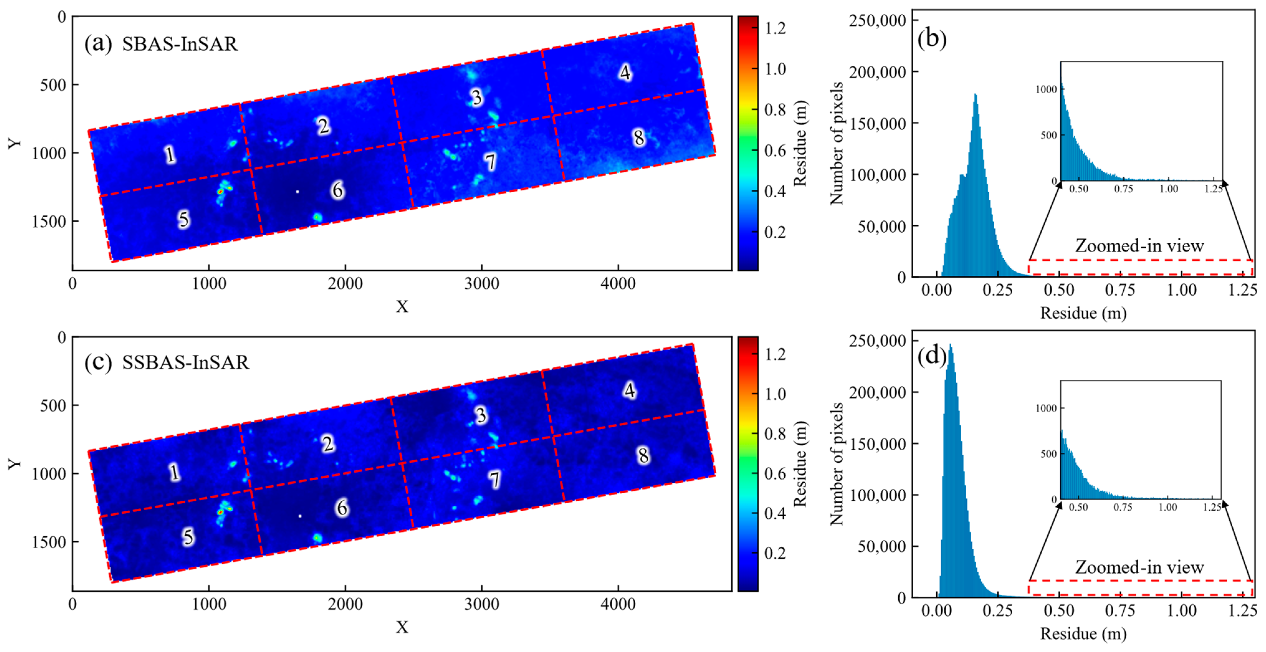
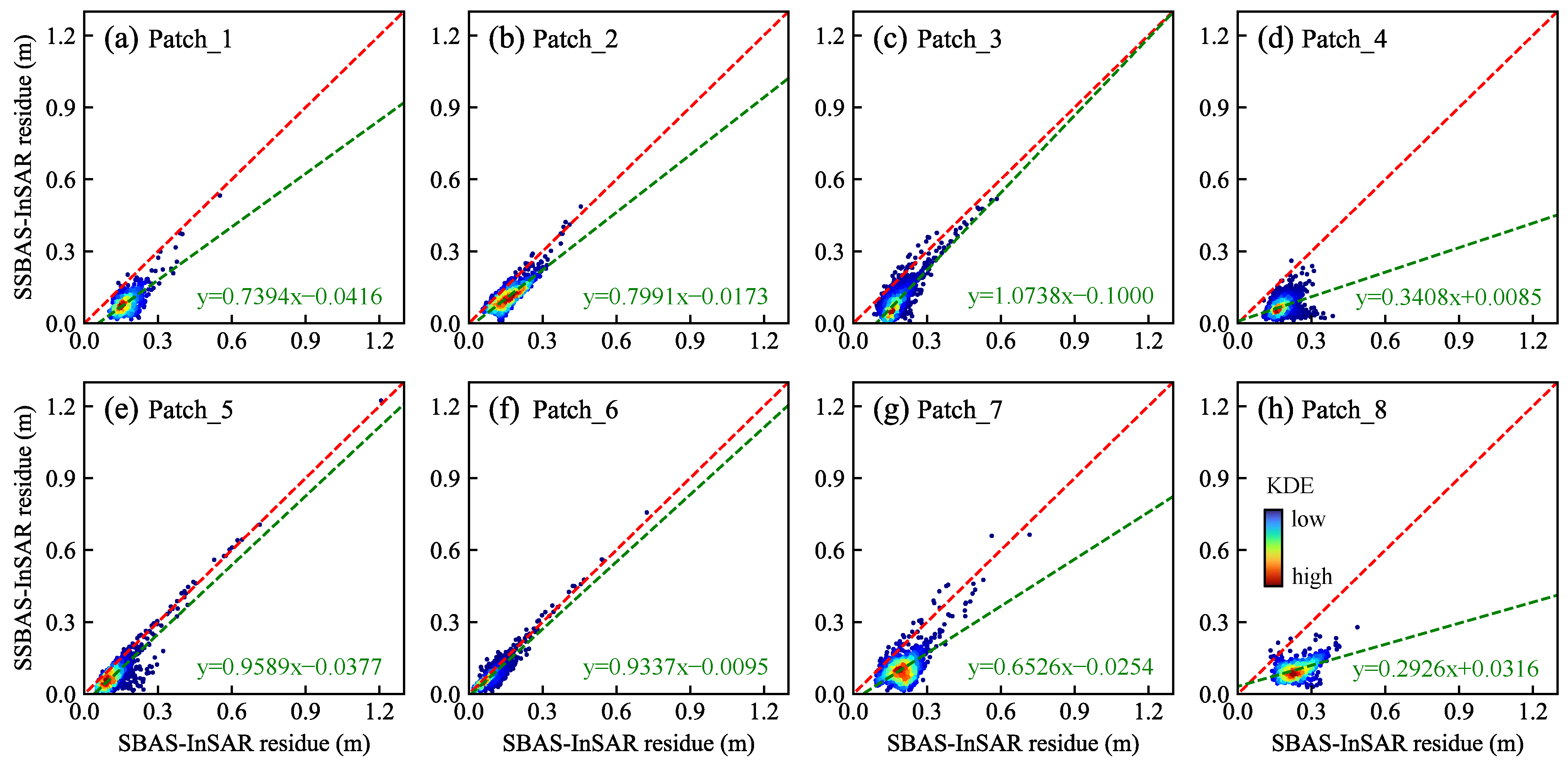
Figure 1. Simulation of phase unwrapping errors. (a) Shows a sample of the simulated interference pattern. (b) Displays a sample of the phase unwrapping result. (c) Illustrates the average absolute phase difference for each block relative to the P1 block, based on 1200 simulations.
Remotesensing 16 03515 g001
Figure 2. Flowchart of SSBAS-InSAR method.
Remotesensing 16 03515 g002
Figure 3. Schematic diagram of phase correction in a local area.
Remotesensing 16 03515 g003
Figure 4. Overview of the study area. (a) Map of the study area. (b) Land cover status, derived from Esri Land Cover 2021 data [36]. (c) Surface elevation of the study area.
Remotesensing 16 03515 g004
Figure 5. Spatiotemporal baseline diagram. The red dots represent SAR imagery. Thanks to the excellent orbital control capability of the Sentinel-1 satellite [38], the 200 m spatial baseline threshold did not exclude any image pairs, ensuring redundancy in the baseline connections and avoiding the introduction of extremely low-coherence data. A total of 369 interferometric pairs were formed.
Remotesensing 16 03515 g005
Figure 6. Data preparation for point selection. (a) Stacking-InSAR deformation rate results. (b) Average coherence graph.
Remotesensing 16 03515 g006
Figure 7. Control point distribution map. The base map shows the Stacking-InSAR deformation rate, with regions of average coherence greater than 0.8. The red rectangle highlights the area within the study region where the absolute value of the Stacking-InSAR deformation rate exceeds 12 cm/year, and the average coherence remains above 0.8.
Remotesensing 16 03515 g007
Figure 8. Examples of multi-control point phase constraints. (a,d,g,j,m,p) The original unwrapped images; (b,e,h,k,n,q) the unwrapped images after applying multi-control point constraints; (c,f,i,l,o,r) the differences between the original unwrapped images and those corrected with multi-control point constraints. The area marked by the red rectangle in (l) indicates where the absolute value of the phase exceeds 20 radians.
Remotesensing 16 03515 g008
Figure 9. Deformation rates obtained from time-series processing. (a) Deformation rate derived using the SBAS-InSAR method. (b) Deformation rate derived using the SSBAS-InSAR method.
Remotesensing 16 03515 g009
Figure 10. Comparison of triangular phase closure. (a,c) The non-zero triangular phase closure numbers of each point of the conventional method and the proposed method, respectively. (b,d) The histograms of the non-zero triangular phase closure numbers of the conventional method and the proposed method, respectively. The unit interval width is 1.
Remotesensing 16 03515 g010
Figure 11. Comparison of temporal coherence. (a,c) The temporal coherence for each point in the conventional SBAS-InSAR method and the proposed SSBAS-InSAR method. (b,d) The corresponding histograms, with a unit interval width of 0.01.
Remotesensing 16 03515 g011
Figure 12. Comparison of the standard deviation of velocity. (a,c) The standard deviation of velocity for each point using the conventional method and the proposed SSBAS-InSAR method, respectively. (b,d) The histograms of the standard deviation of velocity for the conventional method and the proposed method, respectively. The unit interval width is 0.05 mm/year.
Remotesensing 16 03515 g012
Figure 13. Comparison of phase residue. (a,c) The phase residue for each point using the conventional method and the proposed SSBAS-InSAR method, respectively. The red dotted line divides the image into eight regions. (b,d) The histograms of phase residue for the conventional method and the proposed method, respectively. The unit interval width is 0.01 m.
Remotesensing 16 03515 g013
Figure 14. Comparison of phase residue for each patch. (ah) The paches numbered 1 to 8 in Figure 13 (a,c), respectively. The red dotted line in each figure represents y = x, while the green dotted line indicates the linear regression line.
Remotesensing 16 03515 g014
Figure 15. Deformation results for selected areas in Jining. (a) Deformation rate map generated by the SBAS-InSAR method. (b) Deformation rate map generated by the SSBAS-InSAR method. The DEM base map used is GLO-30.
Remotesensing 16 03515 g015
Figure 16. Optical images of the locations of selected points. (a) Optical image of the area where point P1 is located. (b) Optical image of the area where point P2 is located. (c) Optical image of the area where point P3 is located. (d) Optical image of the area where the SDJX point is located.
Remotesensing 16 03515 g016
Figure 17. Comparison of deformation and temperature at point P1. (a,c,e,g) Comparison of time-series deformation and temperature curves obtained through the SBAS-InSAR, SBAS-InSAR+VEC, SBAS-InSAR+DTLF, and SSBAS-InSAR methods, respectively. (b,d,f,h) The correlation coefficient diagrams between deformation and temperature for the four methods, respectively. The red line indicates the linear regression line.
Remotesensing 16 03515 g017
Figure 18. Deformation curve at point P2. (ad) The deformation curves at point P3 obtained by the SBAS-InSAR, SBAS-InSAR+VEC, SBAS-InSAR+DTLF, and SSBAS-InSAR methods, respectively.
Remotesensing 16 03515 g018
Figure 19. Deformation status at point P3. (a) The deformation rate result obtained by the SSBAS-InSAR method. (b) The time-series deformation curves at point P3 obtained by the SBAS-InSAR, SBAS-InSAR+VEC, SBAS-InSAR+DTLF, and SSBAS-InSAR methods.
Remotesensing 16 03515 g019
Figure 20. Location and deformation of GNSS stations. (a) Distribution of GNSS stations in the study area and surrounding regions. (b) Three-dimensional deformation of the SDJX point as observed by GNSS.
Remotesensing 16 03515 g020
Figure 21. Comparison of GNSS deformation results and time-series InSAR results.
Remotesensing 16 03515 g021
Table 1. Average phase residue for each patch (unit: m).
MethodPatch_1Patch_2Patch_3Patch_4Patch_5Patch_6Patch_7Patch_8
SBAS-InSAR0.1767 0.1620 0.1731 0.1788 0.1156 0.0820 0.2034 0.2467
SSBAS-InSAR0.0891 0.1115 0.0854 0.0696 0.0742 0.0668 0.1066 0.1037
Table 2. Characteristics of different time-series InSAR methods.
MethodCharacteristics
SBAS-InSARSingle control point.
SBAS-InSAR+VECSingle control point; linear phase ramp correction; atmospheric phase correction based on GACOS; DEM error phase correction.
SBAS-InSAR+DTLFSingle control point; dual-scale temporal low-pass filtering (small-scale time window size: 36 days, large-scale time window size: 72 days).
SSBAS-InSARMultiple control points.
Table 3. Horizontal movement rates of each GNSS station. The unit is mm/year.
DirectionSDJXHAHBTAINSDLYMaximum Difference
North−11.66−11.65 −11.56 −12.180.62
East31.92 32.02 31.1331.570.89
Disclaimer/Publisher’s Note: The statements, opinions and data contained in all publications are solely those of the individual author(s) and contributor(s) and not of MDPI and/or the editor(s). MDPI and/or the editor(s) disclaim responsibility for any injury to people or property resulting from any ideas, methods, instructions or products referred to in the content.

