Abstract
Global Ecosystem Dynamics Investigation (GEDI) is a relatively new technology for global forest research, acquiring LiDAR measurements of vertical vegetation structure across Earth’s tropical, sub-tropical, and temperate forests. Previous GEDI validation efforts have largely focused on top of canopy accuracy, and findings vary by geographic region and forest type. Despite this, many applications utilize measurements of vertical vegetation distribution from the lower canopy, with a wide diversity of uses for GEDI data appearing in the literature. Given the variability in data requirements across research applications and ecosystems, and the regional variability in GEDI data quality, it is imperative to understand GEDI error to draw strong inferences. Here, we quantify the accuracy of GEDI relative height metrics through canopy layers for the Brazilian Amazon. To assess the accuracy of on-orbit GEDI L2A relative height metrics, we utilize the GEDI waveform simulator to compare detailed airborne laser scanning (ALS) data from the Sustainable Landscapes Brazil project to GEDI data collected by the International Space Station. We also assess the impacts of data filtering based on biophysical and GEDI sensor conditions and geolocation correction on GEDI error metrics (RMSE, MAE, and Bias) through canopy levels. GEDI data accuracy attenuates through the lower percentiles in the relative height (RH) curve. While top of canopy (RH98) measurements have relatively high accuracy (R2 = 0.76, RMSE = 5.33 m), the accuracy of data decreases lower in the canopy (RH50: R2 = 0.54, RMSE = 5.59 m). While simulated geolocation correction yielded marginal improvements, this decrease in accuracy remained constant despite all error reduction measures. Some error rates for the Amazon are double those reported in studies from other regions. These findings have broad implications for the application of GEDI data, especially in studies where forest understory measurements are particularly challenging to acquire (e.g., dense tropical forests) and where understory accuracy is highly important.
1. Introduction
With the launch of the Global Ecosystem Dynamics Investigation (GEDI) mission, Earth observation has an exciting new opportunity to quantify vegetation structure in three dimensions [1]. While the application of Light Detection and Ranging (LiDAR) technology is not new to the field of ecology, it has historically been collected by aircraft, which provides limited spatial coverage, or by the Ice, Cloud, and Land Elevation Satellite (ICESat) which has global coverage but limited accuracy for vegetation [2]. GEDI is designed to bridge that gap by providing samples of vegetation structure within ~25 m diameter footprints along the satellite orbital track, achieving near-global sampling coverage of terrestrial vegetation (between 51.6°N and 51.6°S). GEDI has collected more than 10 billion waveform measurements since its launch in March 2019 [1]. It collected data through early 2023 and is likely to return from hibernation in 2024. The GEDI design is specifically optimized to measure vertical vegetation profiles [1,3], leading to improvements in measurement accuracy of vegetation compared with previous satellite data [2]. These improvements are well documented for canopy height [4] and aboveground biomass [5,6].
While there is significant interest in being able to accurately measure canopy height across the landscape [4,7,8], measures of canopy structure from the bottom half of the vertical distribution of forest vegetation, or hereafter the “lower canopy”, prove crucial in many applications. Aside from measuring canopy height, one of the theoretical benefits of LiDAR is the ability to quantify structure throughout the canopy. In other work, we see that measurements of lower canopy returns appeared crucial in studies that assessed the utility of GEDI in various ecological applications, including avian species distribution models, responses to forest disturbance, and mapping of forest structural diversity [9,10,11,12]. Yet, almost all previous accuracy assessments focused on top of canopy measurements for validation and ignored the lower canopy, apart from one recent study in the contiguous U.S. [13]. Assessing accuracy rates in GEDI measurements throughout the canopy, from the ground to the top of canopy, is an essential consideration for future research applications. Like other satellite datasets, the validation and associated error of GEDI metrics vary across different biomes and regions. For GEDI, these variations are due to biophysical conditions, including steep slopes [2,8,12,14], dense or tall canopies [2,15], and the presence of aerosols. Beam strength, time of data acquisition [2], angle of observation [16], and geolocation error [17,18] also play a role in data quality. GEDI is still a relatively new mission, and footprint geolocation is currently calibrated to within ~10 m (1 σ) accuracy [17], compared to that of ICESat with a mean accuracy of ~3 m [19]. Given all of these influences on data quality, it makes sense that there are considerable discrepancies in the results of GEDI validation studies across different ecosystem types [2,13,16]. Yet, there are over 10,000 current citations on the GEDI datasets [20] and emerging calls to employ GEDI data as a frontier in numerous subdisciplines ranging from global forest mapping and policy applications [21,22,23] to fire research [24,25,26], measuring microclimate [27], and localized biodiversity modeling [10,27]. Given the prevalence of GEDI data within the literature and the regional variability in reported GEDI accuracy, localized validation is imperative to allow for strong inferences to be drawn using these data.
This research focuses on accuracy through two lenses: validation and error minimization. In previous applications, sources of GEDI error were broken down into two broad methods: filtering out GEDI footprints based on sensor/landscape characteristics and the contributions of geolocation error. Approaches that purely use GEDI data and landscape characteristics have used a myriad of approaches that rely on data metrics intrinsic to the GEDI sensor, such as sensitivity, quality flags, and beam strength. These methods have included the exclusion of coverage beams, filtering based on time of observation [2,16], choosing footprints with higher (>0.95) measures of sensitivity [28,29], or removal based on quality flags. Conversely, with the availability of on-orbit GEDI data and high-resolution ALS point clouds, we can simulate the effects of improved geolocation using colocation between the GEDI waveform and hundreds of simulated GEDI-like waveforms derived from spatially concurrent and adjacent ALS data [7,30].
In practice, methods of error minimization rely on different data availability scenarios and sample size needs. While many of the recent applications of GEDI are at a global or continental scale, there is also interest in utilizing GEDI measurements in more localized applications or to assess temporal change [9,24], where GEDI data may be more limited, thus constraining sample size [10,27]. As more of the scientific community begins to utilize GEDI products, a clear understanding of associated errors is essential.
With regional variation and the potential for numerous data constraints, we focused on the Amazon basin, given that it is likely one of the most challenging ecosystems for GEDI applications due to the confluence of canopy height, density, and persistent cloud cover. Remote measurements of the forest structure are critical to our understanding of moist tropical broadleaf systems like the Amazon. Tropical forests are estimated to account for two-thirds of all terrestrial biomass, with the largest deposit of that biomass in the Amazon, which accounts for almost a third of the world’s terrestrial carbon sink [31,32] and is home to an estimated 10% of all species [33] and 62% of terrestrial vertebrates [34]. It has over 13,000 endemic plant species [35,36], ~8000 of which are at high risk of extinction on the ICUN red list [37,38]. Yet the region is also impacted by growing threats to its ecological structure and function [39,40], with ~17% of the forest removed since 1970, and increased rates of deforestation through logging, mining, and fires [40,41,42]. In this region, forest structure is a crucial determinant of carbon storage [43,44] and biodiversity [10,45], but in situ data are difficult to obtain on a meaningful scale. Despite its importance, the Amazon presents additional challenges for remote sensing given the prevalence of cloud cover; tall, dense canopies; and accessibility challenges for validation. These climatic and physical conditions limit the availability of data and may affect their quality. For this reason, coupled with the orbital track of the ISS, the number of high-quality GEDI footprints in the Amazon can be as much as two to six times lower compared to the northern orbital extent [6,28].
In this study, GEDI data are validated by comparing on-orbit GEDI data to simulated GEDI data from fine-scale Airborne Laser Scanning (ALS) data to quantify error rates throughout canopy layers for the Amazonian forest. We also assess the potential for error reduction under two different avenues: the first utilizes GEDI and fine-scale ALS data to simulate geolocation correction, and the second utilizes GEDI attributes and satellite-derived spectral indices (hereafter the “filtering approach”) to select higher quality data. The geolocation correction approach assesses the potential for future improvements with technological and algorithmic tuning advances to improve geolocation. The filtering approach builds on the results of geolocation correction and measures the relative contribution of different common data processing methods on through canopy accuracy. These data filtering scenarios are derived from different methods identified by previous works and are regularly implemented in the current GEDI literature [2,16,18,28,29]. Due to the wide array of error minimization techniques identified by different studies, and the prevalence of relative height values from all canopy layers in GEDI applications [6,9,46], our specific objectives were to (1) validate GEDI relative height data throughout the canopy for the Amazon region and (2) quantify the relative contributions of different data processing methods on error reduction. With this information, the inferences made using GEDI data become more robust, with a better understanding of expected accuracy and the relative distribution of error throughout the canopy.
2. Materials and Methods
2.1. Study Sites
The Sustainable Landscapes Brazil project provides ALS data across Brazil, with collection dates ranging from 2008 to 2018 [47]. For this study, all ALS plots collected in 2018 were considered, and any that fell outside of the South American Moist Tropical Rainforest Biome in Brazil were excluded [48]. This left 36 discrete ALS plots (Table S1) [47,48]. Samples covered three of the largest level II ecoregions in the Brazilian Amazon (Figure S1), including Brazilian Shield Moist Forest to the south, Amazon Lowlands to the North, and Amazon Irregular Plains and Piedmont to the west [49] (Figure 1). The nearly 11,000 hectares within the ALS boundaries is largely forested, with some small areas of opening and agricultural production [50]. A few of the sites were along the banks of the Amazon River, and areas that were water covered were excluded (Figure 1C). The maximum slope encountered in samples was 30 degrees at 1 sample location, but the landscape is otherwise flat (mean slope 4.4 degrees).
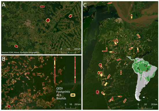
Figure 1.
Study area depicting locations of ALS plots and overlapping GEDI footprints. Zoomed panels (A–C) correspond to letters on the reference map. Green regions on the reference map denote Moist Tropical Broadleaf Biome.
2.2. Data Acquisition
2.2.1. ALS Data
To assess the accuracy of GEDI data for the South American moist tropical rainforest, GEDI data measurements were compared to ALS data provided by the Sustainable Landscapes Brazil Project [47]. All data collected by the Sustainable Landscapes project are quality assured, checked for horizontal and vertical accuracy, and underwent standard quality control after collection [51]. The ALS data used for validation all had high point return densities ranging from an average of 20 to 35 points/m2 (Table S1) and a maximum of 4 returns per shot. ALS data were collected within 1–2 years of GEDI Footprint acquisition, with ALS samples collected in 2018 and GEDI in 2019 or 2020.
Of the 36 ALS plots, all but two plots had GEDI sample overlap. ALS plots cover approximately 10,559 ha across three Brazilian states, Acre, Mato Grosso, and Pará (Figure 1). The sites encompass moist tropical forest and an array of agricultural and edge habitats across the biome. Of the final sample of GEDI footprints, 89% were classified as forest, 1% grassland, and 10% agricultural in 2018 [50].
2.2.2. GEDI Data
GEDI level 2A (L2A) version 002 [52] data were downloaded for the broad region of interest and restricted to the ALS plots after filtering using the L2A quality flag. The L2A quality flag is intended to quickly identify usable data for research applications. Across the 36 ALS sample sites, there were 2693 overlapping GEDI L2A footprints (before any additional data quality checks). Footprints came from 47 orbits, with 39 of those orbits having greater than ten usable footprints overlapping. All L2A default data were retained. The key metrics of interest for validation were relative height (RH) values. RH is derived from the cumulative distribution function of a GEDI waveform centered around the ground return height at 0. As such, RH values represent the height at which a proportion of the GEDI waveform energy has been received from 0 to 100% of the energy in steps of 1% [53] (Figure 2).
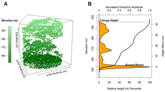
Figure 2.
Depiction of ALS point cloud data (A), corresponding GEDI waveform ((B), orange), and relative height curve ((B), black line).
Additional GEDI metrics of interest included canopy cover and sensitivity. Sensitivity [53] is derived from the ratio of the theoretical minimum detectable ground return energy for a given footprint and waveform algorithm, compared to the total area of that waveform return [54]. Sensitivity is interpreted as a measurement of the maximum canopy cover that a given laser pulse can penetrate and provides a valid ground return for each individual footprint [53]. Given this interpretation, we derived an additional metric termed “sensitivity difference” (sensitivity—canopy cover), such that if canopy cover exceeds sensitivity, the metric yields a negative value. Thus, negative values serve as a flag indicating that the canopy cover may be too dense for the shot to penetrate. Solar elevation for the local time of observation can be used to generate a binary classification of daytime vs. nighttime observations (negative values being nighttime observations). GEDI has two different beam strengths; in any given orbit, half of the ground tracks (8 in total) were collected by a coverage beam and half by a full-power beam. Coverage beams are split to increase the number of samples but, as a byproduct, have reduced power of the along-track measurements, and as such, coverage beams are not as accurate in high canopy coverage conditions. Other information available in this dataset includes a degrade flag intended to indicate footprints that may have degraded positioning information and an elevation bias flag that is similar but pertaining to elevation errors.
2.2.3. Ancillary Data
Given the differences in sample year between ALS and GEDI data acquisition, we accounted for temporal changes by filtering out footprints with any evidence of fire, land use change, or deforestation. To be considered for the analysis, each point had to fall outside of burn perimeters for 2018, 2019, and 2020 if resampled by GEDI in 2020. Additionally, footprints could not have changed in forest canopy cover, detection of forest loss, or transition between landcover types between the ALS sample date and GEDI sample date (Table 1). Where spatial resolution was fine enough that it could be affected by geolocation error, it was coarsened to 90 m.

Table 1.
Ancillary data sources and technical information organized by temporal change category.
Table 1.
Ancillary data sources and technical information organized by temporal change category.
| Type of Change | Data | Source | Temporal Resolution | Dates Used | Resolution (Native and Coarsened) |
|---|---|---|---|---|---|
| Fire | MODIS 500 m burned area monthly | Giglio et al., 2015 [55] | Aggregated to annual | 2018, 2019, 2020 | 500 m |
| CCI burned area | Chuvieco et al., 2018 [56] | Aggregated to annual | 2018, 2019, 2020 | 250 m | |
| Land use change | MAPBIOMAS Brazil landcover | Souza et al., 2020 [57] | Annual | 2018, 2019, 2020 | 30 m coarsened to 90 m |
| Forest loss | Forest loss year | Hansen et al., 2013 [58] | Annual | 2018, 2019, 2020 | 30 m coarsened to 90 m |
The distribution of GEDI sample dates all fell between 20 April and 24 November of their respective years. Thus, the majority of the wet season was not sampled by GEDI, likely due to persistent cloud cover interfering with GEDI sample viability. Additionally, we assessed the trend in GEDI error values across the sample dates present and found no effect. However, we were unable to account for all temporal changes, such as forest growth; for the purposes of this analysis, we assumed that these natural processes did not change the canopy distribution.
2.3. GEDI Simulation
ALS data were converted into a comparable format to the GEDI samples with the widely used GEDI Simulator program to create ~25 m diameter sample footprints at each GEDI sample location (or GEDIsim data) [15]. This program transforms ALS point clouds to GEDI-like waveforms and uses those simulated waveforms to derive relative height metrics [15]. All simulations were done using GEDI Simulator system default parameters, as the default parameters are set to expected GEDI values. The only exceptions were that we used the simulator “check cover” quality flag to omitted points with less than ⅔ ALS cover from all simulations, and we also omitted points with a sensitivity less than 0.9 or densities less than 3 points per square meter from collocation [59]. We maintained relative height outputs from all of the ground finding algorithms available to the simulator (e.g., lowest inflection point, lowest maximum, or Gaussian) and from the ALS identified ground (rhReal). To address the potential consequences of the selection of different algorithms [15], we generated error summaries from all 4 ground finding methods (Figure S2). We report the results based on the Gaussian algorithm, as it is the most widely used and well documented [2,12,13,60]. Nevertheless, there is still an open question about the role of different algorithms for GEDI simulation [60], and we address the implications of our selection in the discussion section. The GEDI Simulator was used to create two distinct datasets, one with simulated waveforms created at the latitude and longitude of the centroid of the L2A footprint as identified in the L2A dataset and one that shifts simulated waveforms based on geolocation error correction (see Section 2.6.1).
2.4. Error Metrics
We used 6 common statistical error metrics to assess the differences between GEDI measurements and ALS-derived GEDIsim values (Equations (1)–(6)). The statistical calculations of error included (1) root mean square error (RMSE), (2) percent root mean square error (RMSE%), (3) mean absolute error (MAE), (4) percent mean absolute error (MAE%) (5) R2 (such that R2 is measured for the expected 1:1 relationship as opposed to a line of best fit with a variable slope; thus we assumed a slope of 1 and intercepting the origin), and (6) bias.
In instances where we did not expect a 1:1 relationship, we report Pearson’s correlation coefficient (r).
where xi is the RH value derived from GEDI, yi is the ALS-derived GEDIsim RH value for comparison, and is the mean of the ALS reference. While we acknowledge each of these metrics has its own problems, these error metrics are widely used and allow for comparison across previous GEDI validation efforts from other regions and the GEDI Simulator program [2,13,15,61]. Additionally, their synthesis allows for strong inference given the wide array of methods utilized.
2.5. Validation
GEDI footprints with quality flags for L2A quality assessment were excluded for validation. GEDI RH values were compared directly to their GEDIsim counterparts (Figure 3, Validation Box). Error, RMSE, RMSE%, R2, and bias were calculated for each paired point for all RH percentiles. RMSE, bias, and R2 were compared to expected error rates intrinsic to the GEDI simulator algorithm [15].
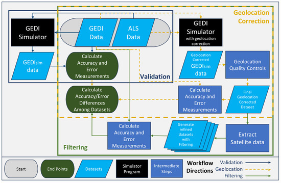
Figure 3.
Workflow of validation and error minimization of on-orbit GEDI data to fine-scale ALS. Nested boxes delineate different processes. All processes begin at the grey oval labelled start in the middle of the diagram and follow color-coded arrows. Validation follows the dark blue arrows within the dark blue box. Both error minimization workflows rely on the validation outputs for comparison. The geolocation correction approach (yellow bounding box) starts at the starting oval with initial data and follows the yellow arrows. The filtering approach (green bounding box) starts with the outputs of the geolocation correction and follows green arrows to the final dataset comparison.
In addition to comparing raw RH values, we calculated the same error metrics for derived canopy metrics of interest. These included Canopy Ratio (), RHsum (,), and the ratio of RH98 to RH50 (). These metrics were selected because they are used in the literature and are of interest for future ecological applications [10,62,63].
2.6. Error Minimization
2.6.1. Geolocation Correction
We measured the contribution of geolocation error to GEDI accuracy by comparing the results of validation of the geolocation-corrected dataset and the validation of the unaltered dataset. The unaltered dataset (with original latitudes and longitudes) served as the baseline for comparison, while the geolocation-corrected dataset (with shifted footprint locations) simulates the effects of increased geolocation accuracy on overall GEDI relative height accuracy.
The geolocation error correction simulates the effects of improved geolocation by uniformly shifting all the footprints in an orbital track around the given initial footprint locations. This shift was first done across a 10 × 10 m grid in 3 m steps [30], and then a simplex approach was used to find the optimum finite shift from the best point in the grid based on 300 iterations [59]. GEDI waveforms were simulated for every footprint in every shifted orbital track. The geolocation correction shift was selected based on the maximization of Pearson’s correlation coefficient between on-orbit GEDI waveform compared to the simulated waveform across the orbital track [15,30] (Figure S3). ALS simulated waveforms were generated using all available algorithms, but the results are reported for the Gaussian algorithm, as it is the most widely used and well documented [2,12,13,60] and thus allows for maximum and direct comparability between studies. Additionally, orbits with fewer than 10 overlapping footprints were omitted from the geolocation corrections, and footprints with an ALS point density less than 5 points per square meter (occurring when footprints were shifted to the edges of ALS tiles) were omitted from the analysis. The 10 footprint cutoff resulted in fewer geolocation-corrected samples than validation samples. The geolocation-corrected results were then compared to the validation results to assess the amount of error reduced by geolocation correction.
2.6.2. Filtering Approach
The geolocation-corrected dataset served as the baseline for the comparison of relative height accuracy after data filtering. Data filters were identified based on the most recent recommendations from GEDI user guides and the results of previous studies in other regions (Table 2). The first filter applied was to remove data flagged as having the potential for elevational bias or geolocation degradation. The resultant dataset serves as the baseline for all subsequent filters. All error measures were made for the filtered datasets and compared to assess error reduction and sample size loss (Figure 3). We also included truncation in the filtering approach, as it is a common practice in GEDI applications, and changed the GEDI data themselves [2]. Truncation is where all negative RH return values (e.g., ground returns) are set to zero. The truncated data were used in generating derived metrics to remove the noise of the ground return.
Table 2.
Proposed data filters and associated sources from the literature.
Table 2.
Proposed data filters and associated sources from the literature.
| Filter | Data Used | Identified By |
|---|---|---|
| Excluding daytime samples | L2A: solar elevation < 0 | Beck et al., (2020) [64]; Fayad et al., (2021) [16] |
| Excluding daytime and coverage beam samples | L2A: solar elevation < 0 and beams | Liu et al., (2021) [2] |
| Sensitivity > 0.95 | L2A: Sensitivity | Beck et al., (2020) [64]; Rishmawi et al., (2021) [29] |
| Excluding coverage beams for canopy cover > 95% | L2A: Beams, GEDIsim: Cover | Beck et al., (2020) [64] |
| Excluding slopes > 30 degrees | ALOS PRISM DEM | Liu et al., (2021) [2] |
| Excluding sensitivity < canopy cover | L2A: Sensitivity, GEDIsim: Cover |
3. Results
3.1. Validation
The R2 values between GEDI RH values and GEDIsim RH values were highest in the top of canopy measures (RH98), while the accuracies consistently decreased in the lower canopy (Figure 4). Our validation was consistent with previous work on LiDAR validation that showed a high variability in RH100 [30]. This trend can be seen in error distribution (Figure 5); the spikes in bias, MAE, and RMSE; and decreases in R2 for RH100 values (Figure 6). As such, we used RH98 to refer to the top of the canopy or canopy height. GEDI data showed a consistent underestimation bias of RH values throughout the canopy (Figure 5). R2 values were much lower than reported GEDI simulator accuracy, with RH98 having the highest R2 (0.76), and that relationship attenuated through the canopy, where RH50 was 0.54 and RH25 was 0.33. R2 yielded negative values below RH12 (Figure 4).
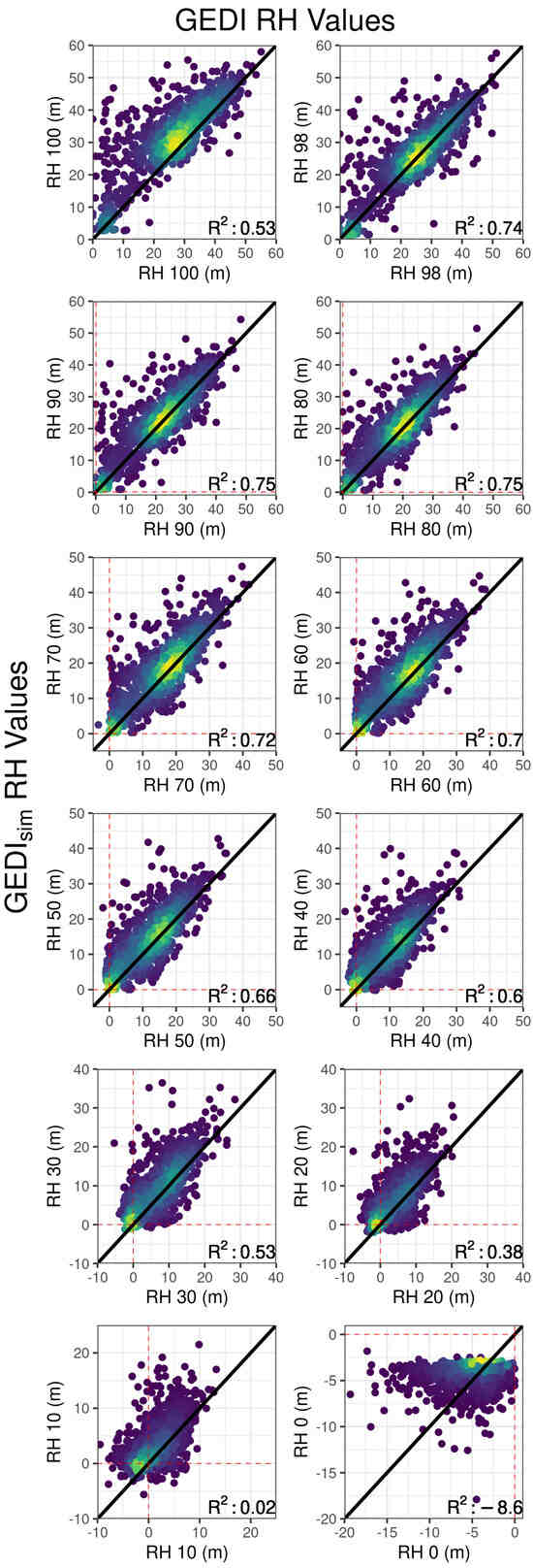
Figure 4.
GEDI-measured RH values compared to their corresponding ALS-derived GEDIsim values starting from RH100 in the top left corner down to RH0 in the bottom right. Point clouds are colored by the density of overlapping points on a scale of yellow (high density) to purple (low density). Black lines indicate where points would fall given a one-to-one relationship between GEDI and GEDIsim. Red dashed lines differentiate negative values from positive.
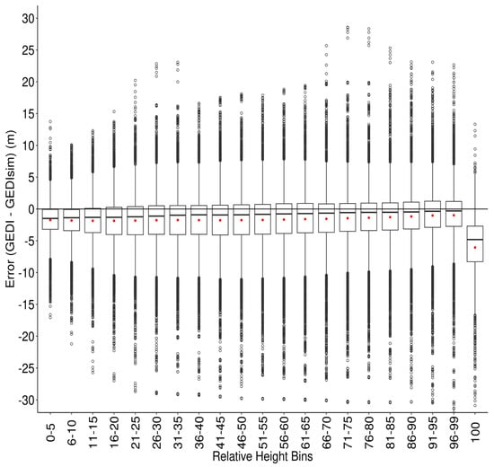
Figure 5.
Box plots of error associated with relative heights. Boxes represent the interquartile range (IQR) (25th percentile of data to the 75th percentile), the black bar is the median, and the red dot is the mean. Error bars extend to 1.5× the IQR, and points are observations outside of that range.
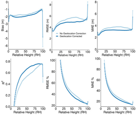
Figure 6.
The relationship between bias, R2, RMSE, RMSE%, MAE, MAE%, and relative height for geolocation-corrected data compared to uncorrected data (quality flags removed). RMSE% values that exceed 100% are not shown, but the general trend persists. Similarly, R2 values below 0 are omitted.
3.2. Geolocation Correction
The distribution of geolocation correction distances had a normal distribution with a mean of 2 m and a 1-sigma of 10 m, closely mirroring the known geolocation error of GEDI [64]. Geolocation corrections yielded lower error metrics through the mid canopy compared to the original dataset. R2 was increased through most of the canopy with geolocation correction, with a maximum increase in R2 of 0.14 at RH32. The threshold at which the R2 value dropped below 0.5 shifted from RH44 to RH28 for uncorrected to geolocation-corrected data, respectively (Figure 6). RMSE and MAE improved slightly with geolocation correction, and error values decreased the most in the mid-canopy compared to top of canopy measures (Table 3). In both geolocation-corrected and uncorrected data, RMSE% and MAE% were both minimized at the top of the canopy and increased as RH decreased (Figure 4). Bias was also inflated (becoming more negative) in the geolocation-corrected dataset below RH85 (Figure 6).
Table 3.
Effects of geolocation correction on error metrics and sample sizes.
3.3. Error Minimization: Filtering
Through the relative height percentiles, agreement between GEDI footprints and simulated ALS relative heights was highest in the upper levels of the canopy (excluding the case of RH100). The R2 coefficient attenuated as RH decreased under all filtering methods (Figure 6). Bias was consistently negative, indicating that GEDI data are underestimating heights compared to the simulated data. Similar to R2, the least bias appeared at RH99 or RH98, and bias values became progressively more negative as RH decreased. RMSE and MAE both increased as RH decreased from the top of the canopy for a period until the height values became uniformly smaller in the lower canopy, resulting in lower RMSE or MAE. However, RMSE% and MAE% showed a monotonic relationship with relative height (Figure 6).
Removal of data with quality flags for geolocation error or elevation estimation error was responsible for the largest error reduction (7.77 to 5.64 and 6.30 to 4.90 RMSE for RH98 and RH50, respectively) (Table 4). This came at the expense of 55% of the initial 2420 usable samples for the region. It is important to note that the dataset with flagged data removed represents the baseline of comparison for all further error reduction.
Table 4.
Error metrics for two relative heights (RH50 and RH98) depending on filtering. Percent Removed is based on the total number of Geolocation corrected footprints. * Indicates baseline for error reduction.
The best results from filtering came from removing footprints where the measure of sensitivity was lower than the measured canopy cover (e.g., where the sensitivity difference <0). This method showed the largest uniform reduction in RMSE, MAE, and Bias and the largest increase in R2 throughout the canopy (Figure 7). Removal of footprints with sensitivity < canopy cover resulted in a shift in the point where the R2 drops below 0.5 from RH28 to RH20 for geolocation-corrected data. Bias also improved by almost an average of 0.55 m uniformly throughout the distribution. However, in excluding these data, the sample size dropped by ~16%, from 1320 samples to 1113 samples. Two other filters showed modest improvements in bias for the lower canopy: filtering out coverage beams with canopy cover >95% and selecting footprints with sensitivity >0.95. Both of those filters reduce the sample size by 8% and 13%, respectively.
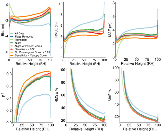
Figure 7.
The relationship between bias, R2, RMSE, RMSE%, MAE, MAE%, and relative height under different scenarios of data filtering. RMSE% values that exceed 100% are not shown, but the general trend persists. Similarly, R2 values below 0 are omitted. * Serves as the baseline condition for all other filters.
3.4. Derived Canopy Metrics
Errors in RH98 and RH50 were only moderately correlated (r = 0.57 in the dataset with no geolocation correction), and methods that reduce error well in the top of the canopy often failed to reduce error meaningfully in the lower canopy (Figure 7). Comparatively, error in the mid to lower canopy had much higher correlation rates (RH25 and RH50, r = 0.84). This lack of strong correlation in error from the upper to the lower levels also has important implications for derived metrics of canopy structure. The higher error in the lower canopy compounded error rates in metrics calculated from multiple RH metrics. For example, in the case of an additive metric such as RHsum, which approximates the area under the RH curve by taking the sum of all positive values of RH, the error compounded to result in an R2 of 0.69 and RMSE of 389 (RMSE% of 32%) for geolocation-corrected data. Metrics that utilize division compounded this problem further and yielded little to no correlation in metrics between GEDI and GEDIsim (Figure 8).
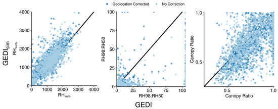
Figure 8.
Canopy metrics calculated from relative height values and the relationship between the GEDI values (x-axis) compared to GEDIsim references (y-axis). All metrics were calculated from truncated data. Left: RHsum, middle: , right: Canopy Ratio = . Points where calculations resulted in values of infinity due to division by zero populate the upper extremes of the plot scales. Black lines indicate where points would fall given a one-to-one relationship.
4. Discussion
4.1. Findings
This study was one of a few studies so far to look at accuracy of relative height metrics throughout the canopy [13]. The highest accuracy was in GEDI’s top of canopy measurements, but this did not persist into the lower canopy. After removing data with quality issues identified by an L2A quality flag, geolocation error flag, and elevation flag, GEDI relative height metrics in the moist tropical forests of Brazil had a RMSE of 5.35 m for top of canopy measurements before geolocation correction with a 95% distribution of error measurements between 12.37 m underestimation and 8.87 m overestimation. The RMSE values from our analysis were similar to the results of another Amazonian study that looked specifically at the effects of algorithm group settings, slope, and terrain on RH95 and RH50 accuracy [65]. In contrast to this study, we assessed accuracies at all RH levels and highlighted the challenges in understory accuracy. In our results, bias showed consistent average underestimations by GEDI. Our through-canopy results contrast with recent findings about GEDI accuracy measured at NEON sites in the contiguous United States [13]. While the bias measurements are comparable, our reported error magnitudes are as much as double those found in the U.S. [13]. The differences between the results from our analysis and those of Wang et al. (2022) are likely due to the fact the forest in the Amazon rainforest is taller, denser, and has more cloud cover than those in the U.S. and thus are inherently more challenging to measure with LiDAR. It is also likely a consequence of these challenges that geolocation flag and elevation flag filtering reduced the sample size by 55%. It is possible that in future versions of GEDI data (currently on version 002), this reduction will be decreased due to more sophisticated geolocation and elevation calibration.
Simulating geolocation correction improved RMSE, MAE, and R2 values in most RH levels. However, it did not change the overall pattern of attenuating accuracy through canopy layers (R2, RMSE%, and MAE%). The geolocation correction did not have much effect on the top of canopy accuracy, likely due to the fact that the majority of sample footprints came from fairly homogeneous forests or agricultural fields, while comparatively few fell along edges or in heterogeneous forests [18]. The lack of change in the pattern of R2, RMSE%, and MAE% from simulated geolocation correction indicates that, though marginal gains may be achieved in mid-canopy accuracy, it is unlikely that additional tuning to the geolocation parameters will correct the overall pattern of decreasing accuracy in the lower canopy.
The filtering approach illuminated inconsistencies compared to the recommendations of the GEDI user guide [66] and the findings of other regional accuracy analyses. Contrary to expectation [2,16], local time of observation and beam strength did not affect accuracy. While Liu et al. (2021) found a reduction in top of canopy RMSE from 3.93 m to 3.56 m by using only measurements taken by full-power beams at night across the contiguous U.S., that was not the case in our study area. This expectation that full-power beams collected at night will yield the best data is built into the GEDI user guide based on the underlying physics of the sensor [66]. Counterintuitively, we found that removing data from daytime samples or daytime samples with coverage beams marginally increased the calculated errors in RH values in the mid and lower canopy. Comparatively, when removing coverage beams with a canopy cover of over 95%, fewer footprints were removed, and there were marginal improvements in R2 and bias metrics. The beam strength and daytime sample results do not support the recommendations of the GEDI data user guide. However, the mechanism for these results is unclear and would need further investigation and comparison across algorithm setting groups. We used the default algorithm setting groups provided in the L2A dataset and did not have sufficient variability across groups to infer their relative contributions to accuracy. Other applications in the region have noted an effect of applying alternative group settings on accuracy [65,67], and the L2A user guide identifies the custom selection of group settings as a potential source of increased local accuracy [64]. The role of alternative algorithm setting group selection remains an open question for through-canopy accuracy in the Amazon.
4.2. Implications
The poor correlation between GEDI and simulated GEDI values in the lower canopy and the limitations of error reduction are critical to understanding future GEDI applications. Previous applications have already used simulated GEDI data to test the utility of GEDI in answering a variety of ecological questions about carbon capacity, species distribution, and disturbance across ecosystems [9,10,11,12,28]. The application of GEDI data for research efforts that pertain to the lower canopy, especially in the moist tropical broadleaf biome, should be taken with care. Furthermore, the applicability of GEDI metrics should be assessed case by case, especially where understory vegetation is the metric of most interest or is a dominant driver of variability in ecological response. Moving forward, comparing effect size and measured GEDI magnitudes of error will be crucial. One such example is the foundational study of forest change in response to hemlock woolly adelgid, where GEDI-simulated data identified forest disturbance [9]. While Boucher et al. 2020 identified RH10 as a strong predictor of disturbance, it would be important to compare the magnitude of change in RH10 to the expected GEDI error for that region.
When using GEDI data and trying to minimize error, there are several considerations when choosing a methodological approach. No matter which method is used, there is an inherent trade-off between data exclusion and sample size. While liberal data filtering may reduce error, it comes at the expense of sample size and potential biases in the dataset. Thus, filters are deeply context dependent. For example, excluding samples based on slope or canopy cover biases the dataset toward flatter or more open forests, and as such, should be considered carefully. Sample size (or density) is also geographically dependent [28], with much higher sample densities at the northern and southern extents of the International Space Station orbit than near the equator or where cloud-free days are limited. While the mean sample density of usable footprints per 1 km cell according to gridded GEDI metrics [68] in the contiguous U.S. was 46, our study region’s sample density was comparatively low at a mean of 17 footprints per 1 km cell [68]. In practice, this means that for our total patchwork ALS coverage of 105 km2, the usable number of footprints from a two-year window was 1345. With data filtering approaches, that sample size was further reduced by up to 50%. Thus, while certain methods may be worthwhile for projects that intend to produce continuous outputs for a large extent, the same methods may be prohibitive for smaller applications.
4.3. Limitations
In assessing GEDI through-canopy error rates, this study followed established methodologies and best practices based on the current state of the literature [15,69,70]. Use of the GEDI Simulator is standard in GEDI validation. However, the simulator itself does not generate perfect comparisons [15]; thus, simulator error undoubtedly influences results. In our comparison of algorithms, we found that the max algorithm showed marginally lower values in error metrics than the Gaussian algorithm. These differences were on the order of tenths of meters, with an average value of 0.13 m lower for both MAE and RMSE. The overall trend in error metrics did not differ beyond these small, uniform shifts in values (Figure S2).
To minimize the influence of simulator error, we only used high point density ALS samples. Additionally, the GEDI Simulator and particularly the Gaussian algorithm are widely used and thus allow for the direct comparison of our measured error rates to other regional studies discussed above [2,12,13,60]. We followed best practices for validation using ALS data [69]. However, even though ALS data are the most commonly used for GEDI performance evaluations [2,7,13,61], and the GEDI simulator was designed for ALS [15], it is impossible to assure that ALS data are a perfect representation of exact field conditions. The ALS data provided from the Sustainable Landscapes Brazil project have been widely used in ecological applications [44,71,72,73,74] and validated against field measurements with high levels of accuracy for canopy height [71,75] and biomass estimates [74]. In foundational studies of ALS accuracy, R2 values for canopy height were consistently high (0.98) [76] and RMSE values low (~1 m) [71,75,76]. Similarly, forest structure has been successfully quantified in previous work [76,77], with accuracy rates for canopy base height (R2 = 0.77), fuel weight (R2 = 0.86), and bulk density (R2 = 0.84) from Anderson et al. (2005). Thus, despite the inability to directly validate GEDI relative height metrics to true ground measurements, we are confident that, despite introducing a small amount of uncertainty, comparison to high-quality ALS provides insight into GEDI error.
4.4. Conclusions
Regional accuracy assessments are a critical resource for future applications of GEDI data. Our results provide error estimates for the Amazon rainforest and illuminate the importance of measuring accuracy throughout the vertical distribution of vegetation. Our results consistently showed that GEDI relative height accuracies decreased through canopy layers; furthermore, some of the error rates recorded in the Amazon are double those found by comparable studies in other regions [13]. As GEDI becomes more widely used, the ecological understanding garnered from interpretation of GEDI data must be disentangled from error rates inherent in the data. This study provides one such benchmark for comparison, but more work is needed to allow for a robust understanding of GEDI accuracies around the globe.
Supplementary Materials
The following supporting information can be downloaded at: https://www.mdpi.com/article/10.3390/rs16193550/s1, Table S1: Information in ALS data; Figure S1: Distribution of GEDI-ALS comparison footprints across US EPA Level 2 ecoregions; Figure S2: Comparison of different ground-finding algorithms from the GEDI Simulator program; Figure S3: Example of geolocation correction; Figure S4: Spatial distribution of canopy height error in GEDI footprints.
Author Contributions
A.E.: Conceptualization, Methodology, Formal analysis, Data Curation, Writing—Original Draft, Visualization, Funding acquisition A.H.: Supervision, Writing—Review and Editing, Conceptualization, Resources P.J.: Supervision, Writing—Review and Editing, Resources, Methodology B.C.: Methodology, Writing—Review and Editing D.W.R.: Methodology, Writing—Review and Editing D.A.: Methodology, Writing—Review and Editing. All authors have read and agreed to the published version of the manuscript.
Funding
This research was partially funded by Montana Space Grant Contortion Graduate Fellowship: 80NSSC20M0042. The APC was funded by the Montana State University Open Access Author Fund.
Data Availability Statement
Data available on request from the authors.
Acknowledgments
This work was supported by the Montana Space Grant Contortion Graduate Fellowship. Computational efforts were performed on the Hyalite High Performance Computing System, operated and supported by University Information Technology Research Cyberinfrastructure at Montana State University.
Conflicts of Interest
The authors declare no conflicts of interest.
References
- Dubayah, R.; Blair, J.B.; Goetz, S.; Fatoyinbo, L.; Hansen, M.; Healey, S.; Hofton, M.; Hurtt, G.; Kellner, J.; Luthcke, S.; et al. The Global Ecosystem Dynamics Investigation: High-Resolution Laser Ranging of the Earth’s Forests and Topography. Sci. Remote Sens. 2020, 1, 100002. [Google Scholar] [CrossRef]
- Liu, A.; Cheng, X.; Chen, Z. Performance Evaluation of GEDI and ICESat-2 Laser Altimeter Data for Terrain and Canopy Height Retrievals. Remote Sens. Environ. 2021, 264, 112571. [Google Scholar] [CrossRef]
- Patterson, P.L.; Healey, S.P.; Ståhl, G.; Saarela, S.; Holm, S.; Andersen, H.E.; Dubayah, R.O.; Duncanson, L.; Hancock, S.; Armston, J.; et al. Statistical Properties of Hybrid Estimators Proposed for GEDI—NASA’s Global Ecosystem Dynamics Investigation. Environ. Res. Lett. 2019, 14, 065007. [Google Scholar] [CrossRef]
- Potapov, P.; Li, X.; Hernandez-Serna, A.; Tyukavina, A.; Hansen, M.C.; Kommareddy, A.; Pickens, A.; Turubanova, S.; Tang, H.; Silva, C.E.; et al. Mapping Global Forest Canopy Height through Integration of GEDI and Landsat Data. Remote Sens. Environ. 2021, 253, 112165. [Google Scholar] [CrossRef]
- Dubayah, R.; Armston, J.; Healey, S.P.; Bruening, J.M.; Patterson, P.L.; Kellner, J.R.; Duncanson, L.; Saarela, S.; Ståhl, G.; Yang, Z.; et al. GEDI Launches a New Era of Biomass Inference from Space. Environ. Res. Lett. 2022, 17, 095001. [Google Scholar] [CrossRef]
- Duncanson, L.; Kellner, J.R.; Armston, J.; Dubayah, R.; Minor, D.M.; Hancock, S.; Healey, S.P.; Patterson, P.L.; Saarela, S.; Marselis, S.; et al. Aboveground Biomass Density Models for NASA’s Global Ecosystem Dynamics Investigation (GEDI) Lidar Mission. Remote Sens. Environ. 2022, 270, 112845. [Google Scholar] [CrossRef]
- Lang, N.; Kalischek, N.; Armston, J.; Schindler, K.; Dubayah, R.; Wegner, J.D. Global Canopy Height Regression and Uncertainty Estimation from GEDI LIDAR Waveforms with Deep Ensembles. Remote Sens. Environ. 2022, 268, 112760. [Google Scholar] [CrossRef]
- Simard, M.; Pinto, N.; Fisher, J.B.; Baccini, A. Mapping Forest Canopy Height Globally with Spaceborne Lidar. J. Geophys. Res. Biogeosci 2011, 116, G04021. [Google Scholar] [CrossRef]
- Boucher, P.B.; Hancock, S.; Orwig, D.A.; Duncanson, L.; Armston, J.; Tang, H.; Krause, K.; Cook, B.; Paynter, I.; Li, Z.; et al. Detecting Change in Forest Structure with Simulated GEDI Lidarwaveforms: A Case Study of the Hemlock Woolly Adelgid (HWA; Adelges Tsugae) Infestation. Remote Sens. 2020, 12, 1304. [Google Scholar] [CrossRef]
- Burns, P.; Clark, M.; Salas, L.; Hancock, S.; Leland, D.; Jantz, P.; Dubayah, R.; Goetz, S.J. Incorporating Canopy Structure from Simulated GEDI Lidar into Bird Species Distribution Models. Environ. Res. Lett. 2020, 15, 095002. [Google Scholar] [CrossRef]
- Qi, W.; Dubayah, R.O. Combining Tandem-X InSAR and Simulated GEDI Lidar Observations for Forest Structure Mapping. Remote Sens. Environ. 2016, 187, 253–266. [Google Scholar] [CrossRef]
- Schneider, F.D.; Ferraz, A.; Hancock, S.; Duncanson, L.I.; Dubayah, R.O.; Pavlick, R.P.; Schimel, D.S. Towards Mapping the Diversity of Canopy Structure from Space with GEDI. Environ. Res. Lett. 2020, 15, 115006. [Google Scholar] [CrossRef]
- Wang, C.; Elmore, A.J.; Numata, I.; Cochrane, M.A.; Shaogang, L.; Huang, J.; Zhao, Y.; Li, Y. Factors Affecting Relative Height and Ground Elevation Estimations of GEDI among Forest Types across the Conterminous USA. GIsci Remote Sens. 2022, 59, 975–999. [Google Scholar] [CrossRef]
- Goetz, S.; Dubayah, R. Advances in Remote Sensing Technology and Implications for Measuring and Monitoring Forest Carbon Stocks and Change. Carbon Manag. 2011, 2, 231–244. [Google Scholar] [CrossRef]
- Hancock, S.; Armston, J.; Hofton, M.; Sun, X.; Tang, H.; Duncanson, L.I.; Kellner, J.R.; Dubayah, R. The GEDI Simulator: A Large-Footprint Waveform Lidar Simulator for Calibration and Validation of Spaceborne Missions. Earth Space Sci. 2019, 6, 294–310. [Google Scholar] [CrossRef]
- Fayad, I.; Baghdadi, N.; Riedi, J. Quality Assessment of Acquired Gedi Waveforms: Case Study over France, Tunisia and French Guiana. Remote Sens. 2021, 13, 3144. [Google Scholar] [CrossRef]
- Luthcke, S.B.; Rebold, T.; Thomas, T.; Pennington, T. Algorithm Theoretical Basis Document (ATBD) for GEDI Waveform Geolocation for L1 and L2 Products, Version 1.0; LP DAAC: Greenbelt, MD, USA, 2019.
- Roy, D.P.; Kashongwe, H.B.; Armston, J. The Impact of Geolocation Uncertainty on GEDI Tropical Forest Canopy Height Estimation and Change Monitoring. Sci. Remote Sens. 2021, 4, 100024. [Google Scholar] [CrossRef]
- Magruder, L.A.; Ricklefs, R.L.; Silverberg, E.C.; Horstman, M.F.; Suleman, M.A.; Schutz, B.E. ICESat Geolocation Validation Using Airborne Photography. IEEE Trans. Geosci. Remote Sens. 2010, 48, 2758–2766. [Google Scholar] [CrossRef]
- LP DACC GEDI L2A: Publications. Available online: https://lpdaac.usgs.gov/resources/publications/?GEDI02_A (accessed on 1 December 2023).
- Hansen, A.J.; Noble, B.P.; Veneros, J.; East, A.; Goetz, S.J.; Supples, C.; Watson, J.E.M.; Jantz, P.A.; Pillay, R.; Jetz, W.; et al. Towards Monitoring Ecosystem Integrity within the Post-2020 Global Biodiversity Framework. Conserv. Lett. 2021, 14, e12822. [Google Scholar] [CrossRef]
- Hansen, A.; Barnett, K.; Jantz, P.; Phillips, L.; Goetz, S.J.; Hansen, M.; Venter, O.; Watson, J.E.M.; Burns, P.; Atkinson, S.; et al. Global Humid Tropics Forest Structural Condition and Forest Structural Integrity Maps. Sci. Data 2019, 6, 232. [Google Scholar] [CrossRef]
- Hansen, A.J.; Burns, P.; Ervin, J.; Goetz, S.J.; Hansen, M.; Venter, O.; Watson, J.E.M.; Jantz, P.A.; Virnig, A.L.S.; Barnett, K.; et al. A Policy-Driven Framework for Conserving the Best of Earth’s Remaining Moist Tropical Forests. Nat. Ecol. Evol. 2020, 4, 1377–1384. [Google Scholar] [CrossRef] [PubMed]
- Fernandez-Manso, A.; Quintano, C.; Roberts, D.A. Burn Severity Analysis in Mediterranean Forests Using Maximum Entropy Model Trained with EO-1 Hyperion and LiDAR Data. ISPRS J. Photogramm. Remote Sens. 2019, 155, 102–118. [Google Scholar] [CrossRef]
- García, M.; North, P.; Viana-Soto, A.; Stavros, N.E.; Rosette, J.; Martín, M.P.; Franquesa, M.; González-Cascón, R.; Riaño, D.; Becerra, J.; et al. Evaluating the Potential of LiDAR Data for Fire Damage Assessment: A Radiative Transfer Model Approach. Remote Sens. Environ. 2020, 247, 111893. [Google Scholar] [CrossRef]
- Liu, M.; Popescu, S.; Malambo, L. Feasibility of Burned Area Mapping Based on ICESAT-2 Photon Counting Data. Remote Sens. 2020, 12, 24. [Google Scholar] [CrossRef]
- Zellweger, F.; De Frenne, P.; Lenoir, J.; Rocchini, D.; Coomes, D. Advances in Microclimate Ecology Arising from Remote Sensing. Trends Ecol. Evol. 2019, 34, 327–341. [Google Scholar] [CrossRef]
- Healey, S.P.; Yang, Z.; Gorelick, N.; Ilyushchenko, S. Highly Local Model Calibration with a New GEDI LiDAR Asset on Google Earth Engine Reduces Landsat Forest Height Signal Saturation. Remote Sens. 2020, 12, 2840. [Google Scholar] [CrossRef]
- Rishmawi, K.; Huang, C.; Zhan, X. Monitoring Key Forest Structure Attributes across the Conterminous United States by Integrating Gedi Lidar Measurements and Viirs Data. Remote Sens. 2021, 13, 442. [Google Scholar] [CrossRef]
- Blair, J.B.; Hofton, M.A. Modeling Laser Altimeter Return Waveforms over Complex Vegetation Using High-Resolution Elevation Data. Geophys. Res. Lett. 1999, 26, 2509–2512. [Google Scholar] [CrossRef]
- Harris, N.L.; Gibbs, D.A.; Baccini, A.; Birdsey, R.A.; de Bruin, S.; Farina, M.; Fatoyinbo, L.; Hansen, M.C.; Herold, M.; Houghton, R.A.; et al. Global Maps of Twenty-First Century Forest Carbon Fluxes. Nat. Clim. Chang. 2021, 11, 234–240. [Google Scholar] [CrossRef]
- Pan, Y.; Birdsey, R.A.; Phillips, O.L.; Jackson, R.B. The Structure, Distribution, and Biomass of the World’s Forests. Annu. Rev. Ecol. Evol. Syst. 2013, 44, 593–622. [Google Scholar] [CrossRef]
- Guayasamin, J.; Ribas, C.; Carnaval, A.; Carrillo, J.; Hoorn, C.; Lohmann, L.; Riff, D.; Ulloa Ulloa, C.; Albert, J.; Nobre, C.; et al. Chapter 2: Evolution of Amazonian Biodiversity. In Amazon Assessment Report 2021; Nations Sustainable Development Solutions Network: New York, NY, USA, 2021. [Google Scholar]
- Pillay, R.; Venter, M.; Aragon-Osejo, J.; González-del-Pliego, P.; Hansen, A.J.; Watson, J.E.M.; Venter, O. Tropical Forests Are Home to over Half of the World’s Vertebrate Species. Front. Ecol. Environ. 2022, 20, 10–15. [Google Scholar] [CrossRef] [PubMed]
- León, B.; Pitman, N.; Roque, J. Introducción a Las Plantas Endémicas del Perú. Rev. Peru. Biol. 2006, 13, 9–22. [Google Scholar] [CrossRef]
- Martins, E.; Martinelli, G.; Loyola, R. Brazilian Efforts towards Achieving a Comprehensive Extinction Risk Assessment for Its Known Flora. Rodriguesia 2018, 69, 1529–1537. [Google Scholar] [CrossRef]
- ICUN. An Introduction to the IUCN Red List of Ecosystems; ICUN: Gland, Switzerland, 2016. [Google Scholar]
- Zapata-Ríos, G.; Andreazzi, C.; Carnaval, A.; Doria, C.; Duponchelle, F.; Flecker, A.; Guayasamín, J.; Heilpern, S.; Jenkins, C.; Maldonado, C.; et al. Chapter 3: Biological Diversity and Ecological Networks in the Amazon. In Amazon Assessment Report 2021; Nations Sustainable Development Solutions Network: New York, NY, USA, 2021. [Google Scholar]
- da Silva, J.M.C.; Rylands, A.B.; da Fonseca, G.A.B. The Fate of the Amazonian Areas of Endemism. Conserv. Biol. 2005, 19, 689–694. [Google Scholar] [CrossRef]
- Silva Junior, C.H.L.; Pessôa, A.C.M.; Carvalho, N.S.; Reis, J.B.C.; Anderson, L.O.; Aragão, L.E.O.C. The Brazilian Amazon Deforestation Rate in 2020 Is the Greatest of the Decade. Nat. Ecol. Evol. 2021, 5, 144–145. [Google Scholar] [CrossRef] [PubMed]
- Holdsworth, A.R.; Uhl, C. Fire in Amazonian Selectively Logged Rain Forest and the Potential for Fire Reduction. Ecol. Appl. 1997, 7, 713–725. [Google Scholar] [CrossRef]
- Uhl, C.; Buschbacher, R. A Disturbing Synergism Between Cattle Ranch Burning Practices and Selective Tree Harvesting in the Eastern Amazon. Biotropica 1985, 17, 265. [Google Scholar] [CrossRef]
- Clark, D.B.; Clark, D.A. Landscape-Scale Variation in Forest Structure and Biomass in a Tropical Rain Forest. For. Ecol. Manag. 2000, 137, 185–198. [Google Scholar] [CrossRef]
- Longo, M.; Keller, M.; dos-Santos, M.N.; Leitold, V.; Pinagé, E.R.; Baccini, A.; Saatchi, S.; Nogueira, E.M.; Batistella, M.; Morton, D.C. Aboveground Biomass Variability across Intact and Degraded Forests in the Brazilian Amazon. Glob. Biogeochem. Cycles 2016, 30, 1639–1660. [Google Scholar] [CrossRef]
- Hyde, P.; Dubayah, R.; Peterson, B.; Blair, J.B.; Hofton, M.; Hunsaker, C.; Knox, R.; Walker, W. Mapping Forest Structure for Wildlife Habitat Analysis Using Waveform Lidar: Validation of Montane Ecosystems. Remote Sens. Environ. 2005, 96, 427–437. [Google Scholar] [CrossRef]
- Ceccherini, G.; Girardello, M.; Beck, P.S.A.; Migliavacca, M.; Duveiller, G.; Dubois, G.; Avitabile, V.; Battistella, L.; Barredo, J.I.; Cescatti, A. Spaceborne LiDAR Reveals the Effectiveness of European Protected Areas in Conserving Forest Height and Vertical Structure. Commun. Earth Environ. 2023, 4, 97. [Google Scholar] [CrossRef]
- Dos-Santos, M.N.; Keller, M.M.; Morton, D.C. LiDAR Surveys over Selected Forest Research Sites, Brazilian Amazon, 2008–2018; ORNL DAAC: Oak RIdge, TN, USA, 2019.
- Dinerstein, E.; Olson, D.; Joshi, A.; Vynne, C.; Burgess, N.D.; Wikramanayake, E.; Hahn, N.; Palminteri, S.; Hedao, P.; Noss, R.; et al. An Ecoregion-Based Approach to Protecting Half the Terrestrial Realm. Bioscience 2017, 67, 534–545. [Google Scholar] [CrossRef] [PubMed]
- US EPA. Level III Ecoregions of Central and South America; US EPA: Washington, DC, USA, 2011.
- Mapbiomas MapBiomas Project—Collection 3 of the Annual Series of Land Cover and Land Use Maps in Brazil. Available online: https://mapbiomas.org/ (accessed on 31 January 2022).
- Dos-Santos, M.N.; Keller, M.M.; Morton, D.C. User Guide: LiDAR Surveys over Selected Forest Research Sites, Brazilian. Amazon, 2008–2018. Available online: https://daac.ornl.gov/CMS/guides/LiDAR_Forest_Inventory_Brazil.html (accessed on 26 May 2022).
- Dubayah, R.; Hofton, M.; Blair, J.B.; Armston, J.; Tang, H.; Luthcke, S. GEDI L2A Elevation and Height Metrics Data Global Footprint Level V002. Available online: https://lpdaac.usgs.gov/products/gedi02_av002/ (accessed on 1 December 2023).
- Beck, J.; Armston, J.; Hofton, M.; Luthcke, S. GLOBAL Ecosystem Dynamics Investigation (GEDI) Level 02 User Guide for SDPS PGE Version 1 (P001) of GEDI L2A Data and SDPS PGE Version 1 (P001) of GEDI L2B Data; LP DAAC: Greenbelt, MD, USA, 2020; Volume 1. Available online: https://lpdaac.usgs.gov/documents/589/GEDIL02_User_Guide_V1.pdf (accessed on 1 March 2022).
- Hofton, M.; Blair, J.B. Algorithm Theoretical Basis Document (ATBD) for GEDI Transmit and Receive Waveform Processing for L1 and L2 Products; Version 1.0.; LP DAAC: Greenbelt, MD, USA, 2019.
- Giglio, L.; Justice, C.; Boschetti, L.; Roy, D. MCD64A1 MODIS/Terra+Aqua Burned Area Monthly L3 Global 500m SIN Grid V006 [Data set]. NASA EOSDIS Land Processes DAAC. LP DAAC: Greenbelt, MD, USA, 2015. [Google Scholar]
- Chuvieco, E.; Pettinari, M.L.; Lizundia-Loiola, J.; Storm, T.; Padilla Parellada, M. ESA Fire Climate Change Initiative (Fire_cci): MODIS Fire_cci Burned Area Pixel Product, version 5.1; 2018. Available online: https://catalogue.ceda.ac.uk/uuid/58f00d8814064b79a0c49662ad3af537/ (accessed on 1 December 2023).
- Souza, C.M.; Shimbo, J.Z.; Rosa, M.R.; Parente, L.L.; Alencar, A.A.; Rudorff, B.F.T.; Hasenack, H.; Matsumoto, M.; Ferreira, L.G.; Souza-Filho, P.W.M.; et al. Reconstructing three decades of land use and land cover changes in brazilian biomes with landsat archive and earth engine. Remote Sens. 2020, 12, 2735. [Google Scholar] [CrossRef]
- Hansen, M.C.; Potapov, P.V.; Moore, R.; Hancher, M.; Turubanova, S.A.; Tyukavina, A.; Thau, D.; Stehman, S.V.; Goetz, S.J.; Loveland, T.R.; et al. High-resolution global maps of 21st-century forest cover change. Science 2013, 342, 850–853. [Google Scholar] [CrossRef]
- Hancock, S. GediSimulator. Available online: https://bitbucket.org/StevenHancock/gedisimulator/src/master/ (accessed on 31 October 2023).
- Leite, R.V.; Silva, C.A.; Broadbent, E.N.; do Amaral, C.H.; Liesenberg, V.; de Almeida, D.R.A.; Mohan, M.; Godinho, S.; Cardil, A.; Hamamura, C.; et al. Large Scale Multi-Layer Fuel Load Characterization in Tropical Savanna Using GEDI Spaceborne Lidar Data. Remote Sens. Environ. 2022, 268, 112764. [Google Scholar] [CrossRef]
- Dhargay, S.; Lyell, C.S.; Brown, T.P.; Inbar, A.; Sheridan, G.J.; Lane, P.N.J. Performance of GEDI Space-Borne LiDAR for Quantifying Structural Variation in the Temperate Forests of South-Eastern Australia. Remote Sens. 2022, 14, 3615. [Google Scholar] [CrossRef]
- East, A.; Hansen, A.; Armenteras, D.; Jantz, P.; Roberts, D.W. Measuring Understory Fire Effects from Space: Canopy Change in Response to Tropical Understory Fire and What This Means for Applications of GEDI to Tropical Forest Fire. Remote Sens. 2023, 15, 696. [Google Scholar] [CrossRef]
- Ferrer Velasco, R.; Lippe, M.; Tamayo, F.; Mfuni, T.; Sales-Come, R.; Mangabat, C.; Schneider, T.; Günter, S. Towards Accurate Mapping of Forest in Tropical Landscapes: A Comparison of Datasets on How Forest Transition Matters. Remote Sens. Environ. 2022, 274, 112997. [Google Scholar] [CrossRef]
- Beck, J.; Wirt, B.; Armston, J.; Hofton, M.; Luthcke, S.; Tang, H. GLOBAL Ecosystem Dynamics Investigation (GEDI) Level 2 User Guide; Verson 2.0; LP DAAC: Greenbelt, MD, USA, 2021; Volume 3, pp. 1–25.
- Oliveira, V.C.P.; Zhang, X.; Peterson, B.; Ometto, J.P. Using Simulated GEDI Waveforms to Evaluate the Effects of Beam Sensitivity and Terrain Slope on GEDI L2A Relative Height Metrics over the Brazilian Amazon Forest. Sci. Remote Sens. 2023, 7, 100083. [Google Scholar] [CrossRef]
- Beck, J.; Luthcke, S.B.; Hofton, M.; Armstron, J. GLOBAL Ecosystem Dynamics Investigation (GEDI) Level 1B User Guide; Version 1.0.; LP DAAC: Greenbelt, MD, USA, 2020; Volume 1.
- Lahssini, K.; Baghdadi, N.; le Maire, G.; Fayad, I. Influence of GEDI Acquisition and Processing Parameters on Canopy Height Estimates over Tropical Forests. Remote Sens. 2022, 14, 6264. [Google Scholar] [CrossRef]
- Dubayah, R.O.; Luthcke, S.B.; Sabaka, T.J.; Nicholas, J.B.; Preaux, S.; Hofton, M.A. GEDI L3 Gridded Land Surface Metrics, Version 2; ORNL DAAC: Oak RIdge, TN, USA, 2021.
- Duncanson, L.; Armston, J.; Disney, M.; Avitabile, V.; Barbier, N.; Calders, K.; Carter, S.; Chave, J.; Herold, M.; MacBean, N.; et al. Aboveground Woody Biomass Product Validation Good Practices Protocol. In Good Practices for Satellite Derived Land Product Validation; Duncanson, L., Disney, M., Armston, J., Nickeson, J., Minor, D., Camacho, F., Eds.; Committee on Earth Observation Satellites Working Group on Calibration and Validation: Geneva, Switzerland, 2021. [Google Scholar]
- NASA. University of Maryland GEDI Ecosystem LiDAR Calibration/Validation. Available online: https://gedi.umd.edu/science/calibration-validation/ (accessed on 1 June 2022).
- Hunter, M.O.; Keller, M.; Victoria, D.; Morton, D.C. Tree Height and Tropical Forest Biomass Estimation. Biogeosciences 2013, 10, 8385–8399. [Google Scholar] [CrossRef]
- Rappaport, D.I.; Morton, D.C.; Longo, M.; Keller, M.; Dubayah, R.; Dos-Santos, M.N. Quantifying Long-Term Changes in Carbon Stocks and Forest Structure from Amazon Forest Degradation. Environ. Res. Lett. 2018, 13, 065013. [Google Scholar] [CrossRef]
- Sato, L.Y.; Gomes, V.C.F.; Shimabukuro, Y.E.; Keller, M.; Arai, E.; dos-Santos, M.N.; Brown, I.F.; de Aragão, L.E.O.E.C. Post-Fire Changes in Forest Biomass Retrieved by Airborne LiDAR in Amazonia. Remote Sens. 2016, 8, 839. [Google Scholar] [CrossRef]
- Silva, C.A.; Hudak, A.T.; Vierling, L.A.; Klauberg, C.; Garcia, M.; Ferraz, A.; Keller, M.; Eitel, J.; Saatchi, S. Remote Sensing Impacts of Airborne Lidar Pulse Density on Estimating Biomass Stocks and Changes in a Selectively Logged Tropical Forest. Remote Sens. 2017, 9, 1068. [Google Scholar] [CrossRef]
- Leitold, V.; Keller, M.; Morton, D.C.; Cook, B.D.; Shimabukuro, Y.E. Airborne Lidar-Based Estimates of Tropical Forest Structure in Complex Terrain: Opportunities and Trade-Offs for REDD+. Carbon. Balance Manag. 2014, 10, 3. [Google Scholar] [CrossRef] [PubMed]
- Andersen, H.E.; McGaughey, R.J.; Reutebuch, S.E. Estimating Forest Canopy Fuel Parameters Using LIDAR Data. Remote Sens. Environ. 2005, 94, 441–449. [Google Scholar] [CrossRef]
- Lefsky, M.A.; Cohen, W.B.; Acker, S.A.; Parker, G.G.; Spies, T.A.; Harding, D. Lidar Remote Sensing of the Canopy Structure and Biophysical Properties of Douglas-Fir Western Hemlock Forests. Remote Sens. Environ. 1999, 70, 339–361. [Google Scholar] [CrossRef]
Disclaimer/Publisher’s Note: The statements, opinions and data contained in all publications are solely those of the individual author(s) and contributor(s) and not of MDPI and/or the editor(s). MDPI and/or the editor(s) disclaim responsibility for any injury to people or property resulting from any ideas, methods, instructions or products referred to in the content. |
© 2024 by the authors. Licensee MDPI, Basel, Switzerland. This article is an open access article distributed under the terms and conditions of the Creative Commons Attribution (CC BY) license (https://creativecommons.org/licenses/by/4.0/).