A Robust Translational Motion Compensation Method for Moving Target ISAR Imaging Based on Phase Difference-Lv’s Distribution and Auto-Cross-Correlation Algorithm

Abstract

Translational motion compensation constitutes a pivotal and essential procedure in inverse synthetic aperture radar (ISAR) imaging. Many researchers have previously proposed their methods to address this requirement. However, conventional methods may struggle to produce satisfactory results when dealing with non-stationary moving targets or operating under conditions of low signal-to-noise ratios (SNR). Aiming at this challenge, this article proposes a parametric non-search method that contains two main stages. The radar echoes can be modeled as polynomial phase signals (PPS). In the initial stage, the energy of the received two-dimensional signal is coherently integrated into a peak point by leveraging phase difference (PD) and Lv’s distribution (LVD), from which the high-order polynomial coefficients can be obtained accurately. The estimation of the first-order coefficients is conducted during the second stage. The auto-cross-correlation function for range profiles is introduced to enhance the accuracy and robustness of estimation. Subsequently, a novel mathematical model for velocity estimation is proposed, and its least squares solution is derived. Through this model, a sub-resolution solution can be obtained without requiring interpolation. By employing all the estimated polynomial coefficients, the non-stationary motion of the target can be fully compensated, yielding the acquisition of a finely focused image. Finally, the experimental findings validate the superiority and robustness of the proposed method in comparison to state-of-the-art approaches.

1. Introduction

As an active microwave remote sensor that can ignore all weather and sunlight conditions and produce valuable images, inverse synthetic aperture radar (ISAR) plays a significant role in all countries today [1,2]. In ISAR imaging, wideband signals are transmitted by the radar system to reach high range resolution, and coherent integration is leveraged to actualize high cross-range (azimuth) resolution [3,4]. The relative motion between the observed target and the radar system enables the acquisition of a clear two-dimensional (2D) image of the target [5]. In actual application and practice, the observed target is always non-cooperative [6], and the target’s motion can be treated as a composition of translational motion and rotational motion. However, not all motion components contribute to the imaging process. According to the ISAR rotation imaging model [7], the rotational motion component of the target under observation may provide the requisite Doppler frequency gradient for the creation of a high-resolution image, whereas the translational motion component not only lacks benefit but also introduces issues concerning range cell migration and phase errors, consequently leading to image degradation. The primary objectives of ISAR imaging are typically target detection [8,9] and recognition [8,10,11], which are essential for accurate image interpretation. High image quality is a prerequisite for all subsequent tasks, and motion compensation is an essential and preliminary step in obtaining high-quality images. Hence, to achieve a high-quality ISAR image of the target, it is imperative to adequately compensate for the translational motion of the target to the greatest extent feasible [12,13]. While numerous methods have been devised to address this issue [14,15,16,17], they often fail to yield satisfactory outcomes in low signal-to-noise ratio (SNR) environments, notably concerning prominent targets such as maritime vessels and stealth fighters, which hold significant importance in ISAR applications. Therefore, achieving perfect compensation for translational motion in low SNR environments poses a significant practical challenge and represents a valuable area for research.

The process of translational motion compensation typically encompasses range alignment and phase adjustment (autofocus) [18,19,20]. Range alignment ensures that scatterers remain within a specific range cell. When the SNR reaches a sufficient level, the correlation between the adjacent echoes is markedly elevated. Founded on this fact, the maximum correlation range alignment (MCRA) method [20] can be deployed to align the range profiles. However, this method has trouble concerning error accumulation and is sensitive to the target glint effect. Moreover, it is not applicable under conditions of low SNR due to the absence of similarity between adjacent echoes. To enhance the stability of the MCRA method, the global range alignment (GRA) method [21] and the improved global range alignment (IGRA) method [22] have been introduced. These approaches align the range profiles based on the sum/average of each, thereby augmenting their suitability and effectiveness. The sharpness of the 2D range profiles will be maximized if the whole profiles are aligned accurately; hence, several optimization-based methods [23,24,25] are proposed with the contrast/entropy criteria. However, these approaches [21,22,23,24,25] only use the range profiles’ magnitude information and fall into the non-coherent integration methods, exhibiting a poor anti-noise performance. Moreover, these methods correct the range profiles to half of the range resolution, resulting in insufficient accuracy and necessitating interpolation in practical applications, thereby imposing an additional computational burden. There are few methods that can effectively address the low SNR scenario with a high level of accuracy, which is a motivating factor for us.

Phase adjustment is conducted after range alignment to linearize the phase history. Generally, the phase adjustment methods can be categorized broadly into two diverse classes: nonparametric and parametric. The dominant scatterers method [26] and phase gradient autofocus (PGA) method [27] belong to the nonparametric category, and they can achieve satisfactory results under conditions of stationary target motion and adequate SNR. Unfortunately, these methods rely heavily on the target’s dominant scattering center, which may be troublesome to extract in scenarios of deteriorating SNR. The PGA method necessitates iterative computations, incurring computational expenses. For better robustness, image quality-based parametric methods are developed [28,29,30]. When the phase adjustment is performed perfectly, the quality of the ISAR image will be the best. The above parametric methods commonly optimize the phase error with the goal of contrast maximum [28,29] or entropy minimum [30]. The efficacy of these optimization techniques in mitigating noise is excellent with the aid of the SNR gain achieved through coherent integration in the azimuth direction. However, their high computational burden is universal, and their performance is closely linked with the range alignment. Only if the range alignment is delivered accurately can the image quality-based methods be valid. This prerequisite raises a higher requirement for the accuracy of the range alignment.

Essentially, the translational motion of a moving target leads to both range migration and phase errors, presenting an opportunity for simultaneous compensation of both. Various parametric approaches [31,32,33] are introduced using translational motion modeling to realize joint range alignment and phase adjustment. These methods can take full advantage of the SNR gain of 2D coherent integration, carrying a better anti-noise performance, but they still exhibit certain limitations. The maximum contrast range alignment method [31] devises an iterative search approach to estimate model parameters by maximizing image contrast. However, the modeling of range translational motion solely as a second-order polynomial function in this approach may result in potential mismatching between the model and practical scenarios, thereby imposing significant constraints on the method’s applicability. In reference [32], an advanced high-order polynomial function was formulated to characterize the translational motion, offering a more apposite depiction of the observed moving target. What’s more, it introduced the minimum entropy image quality evaluation metric (IQEM) as a cost function to estimate the polynomial coefficients and designs with a quasi-Newton-based algorithm to attain the optimal solution. However, due to the non-convex nature of the IQEM function, there remains a possibility that the method may converge towards a local optimal solution, particularly under the low SNR scenario. To avoid falling into a local optimal solution, particle swarm optimization (PSO) is employed to facilitate the attainment of a global optimal solution, and the combined IQEM-PSO method [33] is proposed. However, there are still some notable constraints for this method. The computational demands of the PSO method remain particularly onerous, thus precluding the system from accommodating real-time requirements. In addition, the IQEM struggles to correctly characterize images’ quality under low SNR scenarios. The two constraints are presumed to result in a compensation defeat and the degradation of the generated ISAR image.

Inspired by prior research and persistent challenges, this paper proposes a parametric non-search approach based on phase difference-Lv’s distribution and an auto-cross-correlation algorithm for ISAR translational motion compensation that spares no effort to enhance the SNR gain. To ensure the accuracy of this model, a third-order polynomial function is employed to represent the translational motion of the target; thus, the target’s velocity, acceleration, and acceleration rate are all taken into account. With the assistance of the third-order model, the proposed method can achieve joint range alignment and phase adjustment feasibly, thus making the 2D coherent integration gain a reality. In addition, the moving target can be treated as a rigid body, and the scatterers share the same translational motion parameters that do not concern the scatterers’ individual positions. Based on this fact, the phase difference (PD) operation is leveraged to coherently convert the received 2D signal power to the one-dimensional (1D) compressive range cell signal during the first stage of the proposed method. Meanwhile, the keystone transform (KT) plays a pivotal role in intensifying SNR gain. Lv’s distribution (LVD) [34] follows the PD operation and the KT transform to coherently transform the 1D chirp signal to a peak point. LVD is a powerful tool for the analysis of non-stationary signals [34,35]. After two coherent integrations, the energy of the received signal is integrated into a peak point, indicating the strong robustness of the method and the accurate estimation of the high-order polynomial coefficients. In the next stage, to estimate the first-order polynomial coefficients accurately and robustly, the auto-cross-correlation function (ACCF) for range profiles is defined, which is more robust than the cross-correlation function (CCF). Benefiting from the ACCF, a novel mathematical optimization model for first-order parameter estimation is developed, and its least squares (LS) solution is derived to achieve a sub-resolution level without interpolation and searching, namely the auto-cross-correlation algorithm (ACCA). With all the estimated polynomial coefficients, the non-stationary motion of the target can be fully compensated using the compensation function, yielding the appearance of a clear and focused ISAR image. Finally, the experimental findings validate the superiority and robustness of the proposed method compared to state-of-the-art approaches.

The remainder of this article is organized as follows. Section 2 establishes the cubic phase signal model of ISAR imaging for a non-stationary moving target. The proposed translational motion compensation method is introduced in detail in Section 2.2 where the PD-LVD and ACCA methods are employed to estimate the translational motion parameters. Section 3 demonstrates several measured data processing results by different approaches to validate the proposed method’s superiority, and Section 4 offers a comparative analysis and discussion on the outcomes of alternative methods alongside the proposed approach. Finally, Section 5 presents the conclusions.

2. Materials and Methods

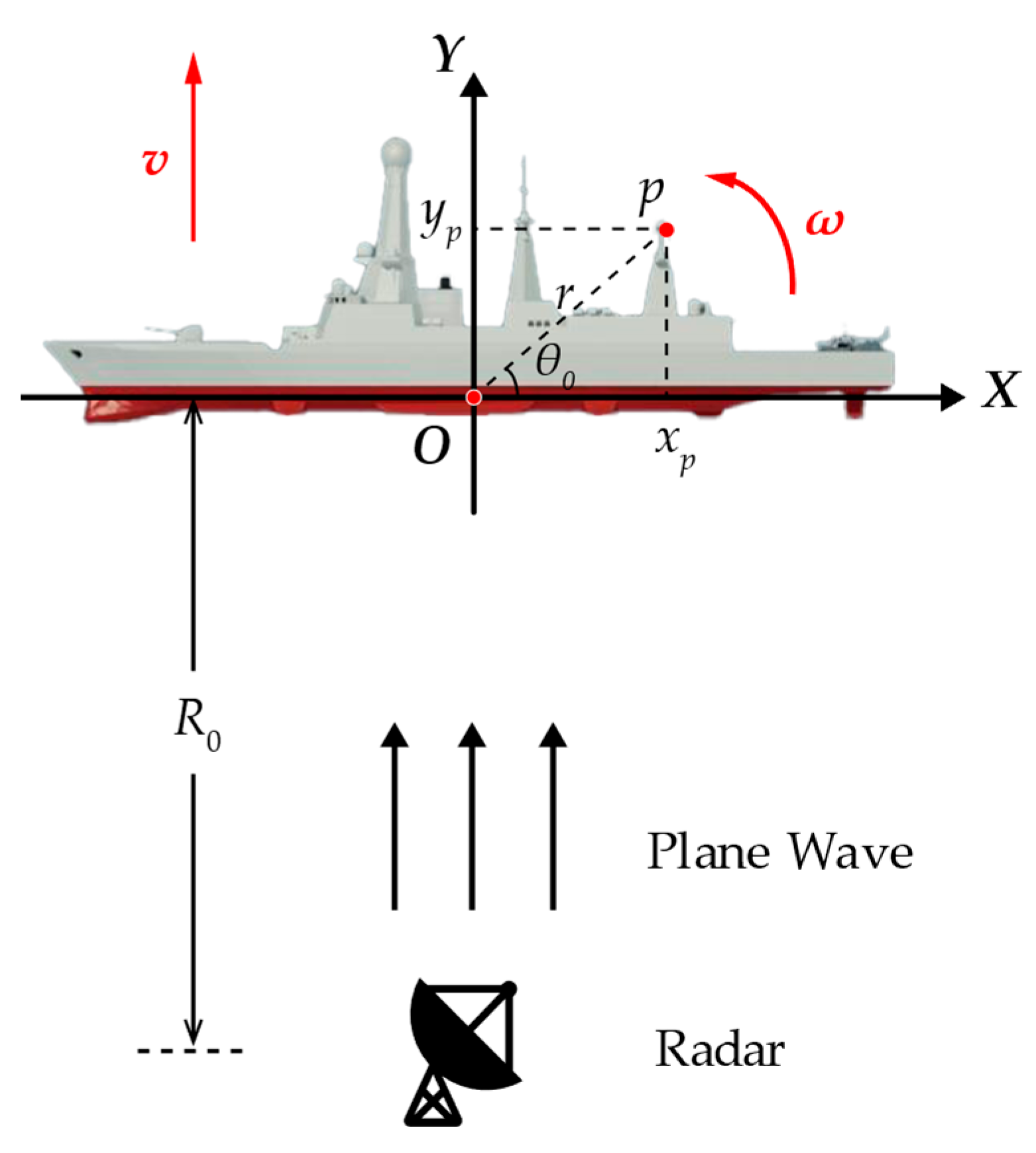
2.1. ISAR Imaging Geometry and Cubic Phase Signal Model

This section focuses on ISAR imaging geometry and establishes the cubic phase signal model for a non-stationary moving target. Figure 1 illustrates the classic ISAR imaging geometry model of a moving target, where OXY is a target body Cartesian coordinate system. Point O is the origin of OXY as well as the rotational center in the observed target, assuming that the target contains P scatterers and point p represents the pth scatterer whose coordinate is $\left(x_p,y_p\right)$. The physical motion of the target can be considered as the combination of the translation and rotation motions, and $v$ and $\omega$ represent these two motions, respectively. Without losing generality, this thesis focuses on translational motion, and the target can be regarded as rotating uniformly, meaning the angular velocity $\omega$ is just a constant.

For the ISAR system, chirp signal usually plays the transmitting signal role [36,37], and its mathematical expression is

$$s_t\left(t\right)=\mathrm{rect}\left({\displaystyle \frac{\widehat{t}}{T_p}}\right)\exp \left\{\mathrm{j}2\pi \left(f_{c}t+{\displaystyle \frac{1}{2}}\mu {\widehat{t}}^2\right)\right\},$$

(1)

where $T_p$ is the pulse width, $\widehat{t}\in \left[-T_p/2,T_p/2\right]$ is the fast time, $t$ is the full time, $f_c$ is the transmitting frequency of the system, $\mu$ is the chirp rate of the transmitted signal, and $\mathrm{rect}\left(\ast \right)$ is defined as

$$\mathrm{rect}\left(u\right)=\left\{\begin{array}{c}1 \left|u\right|\le 1/2\\ 0 \left|u\right|>1/2\end{array}\right., u\in \mathbf{R}.$$

(2)

The full-time variable $t$ meets $t=t_m+\widehat{t}$, where $t_m$ stands for the slow time. Assuming N is the number of pulses and $\Delta T$ is the pulse repetition interval (PRI), $t_m$ can be expressed as $n\cdot \Delta T,n=0,1,2,\cdots ,N-1$.

After undergoing demodulation processing by the receiver, the echo signal is shifted to the baseband, which can be expressed in terms of $\widehat{t}$ and $t_m$ as follows:

$$s_r\left(\widehat{t},t_m\right)={\displaystyle \sum _{p=1}^P{\sigma }_p\mathrm{rect}\left(\frac{\widehat{t}-\frac{2R_p\left(t_m\right)}{c}}{T_p}\right)}\exp \left\{\mathrm{j}\mathsf{\pi }\mu {\left(\widehat{t}-{\displaystyle \frac{2R_p\left(t_m\right)}{c}}\right)}^2\right\}\exp \left\{-\mathrm{j}4\mathsf{\pi }{\displaystyle \frac{R_p\left(t_m\right)}{\lambda }}\right\},$$

(3)

where ${\sigma }_p$ is the reflection coefficient of the pth scatterer, $R_p\left(t_m\right)$ is the range distance from the radar to the pth scatterer, c represents the velocity of light, and $\lambda$ is the wavelength of the transmitted electromagnetic wave.

According to the principle of stationary phase (POSP), the frequency response function of the transmitted chirp signal can be written as (4) approximately:

$$U\left(f\right)={\displaystyle \frac{1}{\sqrt{\mu }}}\mathrm{rect}\left({\displaystyle \frac{f}{B}}\right)\exp \left\{-\mathrm{j}{\displaystyle \frac{\pi }{\mu }}{f}^2\right\},$$

(4)

where f is the frequency variable, and $B=\mu T_p$ is the bandwidth of the chirp signal, similar to (1).

By conducting Fourier Transform (FT) concerning the fast time $\widehat{t}$ based on (4), the received signal form in the range-frequency slow-time domain is derived as

$$\begin{array}{cc}\hfill S\left(f_r,t_m\right)& ={\displaystyle \sum _{p=1}^P{\sigma }_{p}U\left(f_r\right)\exp \left\{-\mathrm{j}2\pi f_r\frac{2R_p\left(t_m\right)}{c}\right\}\exp \left\{-\mathrm{j}4\pi \frac{f_c}{c}{R}_p\left(t_m\right)\right\}}\hfill \\ & ={\displaystyle \sum _{p=1}^P{\sigma }_{p}U\left(f_r\right)\exp \left\{-\mathrm{j}4\pi \frac{f_r+f_c}{c}{R}_p\left(t_m\right)\right\}}\hfill \end{array},$$

(5)

where $f_r$ is the range frequency variable and the equality $\lambda =c/f_c$ is involved in the derivation.

Matching filtering is employed to realize the goal of range compression, and the compressed signal is shown in (6):

$$S\left(f_r,t_m\right)={\displaystyle \sum _{p=1}^P{\sigma }_p^{\prime }\exp \left\{-\mathrm{j}4\pi \frac{f_r+f_c}{c}{R}_p\left(t_m\right)\right\}},$$

(6)

where ${\sigma }_p^{\prime }={\sigma }_p{\left|U\left(f_r\right)\right|}^2$.

The detection distance of the ISAR system always satisfies the far field condition, so the electromagnetic wave that hits the target can be seen as a plane wave. Hence, the instantaneous range distance from the radar to the pth scatterer can be approximated as

$$R_p\left(t_m\right)\approx R_o\left(t_m\right)+r\sin \theta \left(t_m\right),$$

(7)

where $R_o\left(t\right)$ is the instantaneous range distance from the radar to the rotational center O, and $\left(r,\theta \left(t_m\right)\right)$ is the instantaneous polar coordinate of the pth scatterer whose initial Cartesian coordinate is $\left(x_p,y_p\right)$. The instantaneous polar angle $\theta \left(t_m\right)$ consists of the initial polar angle and the rotation angle at time $t_m$.

Assuming the initial polar angle is ${\theta }_0$, it is readily observed that (8) holds:

$$\left\{\begin{array}{l}{x}_p=r\cos {\theta }_0\\ y_p=r\sin {\theta }_0\end{array}\right..$$

(8)

Assuming ${\theta }_{\omega }\left(t_m\right)$ represents the real-time rotation angle, according to (7) and (8), $R_p\left(t_m\right)$ can be rewritten as

$$\begin{array}{cc}\hfill R_p\left(t_m\right)& \approx R_o\left(t_m\right)+r\sin \left({\theta }_0+{\theta }_{\omega }\left(t_m\right)\right)\hfill \\ & =R_o\left(t_m\right)+y_p\cos \left({\theta }_{\omega }\left(t_m\right)\right)+x_p\sin \left({\theta }_{\omega }\left(t_m\right)\right)\hfill \end{array}.$$

(9)

In fact, ${\theta }_{\omega }\left(t_m\right)$ is usually small (3°~5°) [24], so the approximations in (10) are available [38].

$$\left\{\begin{array}{c}\cos \left({\theta }_{\omega }\left(t_m\right)\right)\approx 1\hfill \\ \sin \left({\theta }_{\omega }\left(t_m\right)\right)\approx {\theta }_{\omega }\left(t_m\right)\hfill \end{array}\right..$$

(10)

While $R_o\left(t_m\right)$ contains the initial range distance $R_0$ and the translation distance $R_T\left(t_m\right)$, substituting (10) into (9) yields

$$R_p\left(t_m\right)\approx R_0+R_T\left(t_m\right)+y_p+x_p{\theta }_{\omega }\left(t_m\right).$$

(11)

For an ideal ISAR rotating imaging model [7], $R_T\left(t_m\right)$ and ${\theta }_{\omega }\left(t_m\right)$ are expected to be 0 and $\omega t_m$, respectively, where $\omega$ is the angular velocity. In this circumstance, $R_p\left(t_m\right)$ is turned into

$$R_p\left(t_m\right)\approx R_0+y_p+x_p\omega t_m.$$

(12)

Substituting (12) into (6) yields

$$S\left(f_r,t_m\right)={\displaystyle \sum _{p=1}^P{\sigma }_p^{\prime }\exp \left\{-\mathrm{j}4\pi \frac{f_r+f_c}{c}\left(R_0+y_p+x_p\omega t_m\right)\right\}}.$$

(13)

Subsequently, the signal form in the fast-time slow-frequency domain is acquired using the FT and inverse FT (IFT), as illustrated in (14):

$$S\left(\widehat{t},f_m\right)={\displaystyle \sum _{p=1}^P{\sigma }_p^{\prime }\sin \mathrm{c}}\left\{B\left(\widehat{t}-{\displaystyle \frac{2\left(R_0+y_p+x_p\omega t_m\right)}{c}}\right)\right\}\sin \mathrm{c}\left\{T_d\left(f_m-{\displaystyle \frac{2x_p\omega }{\lambda }}\right)\right\},$$

(14)

where $f_m$ is the slow frequency variable and $T_d$ is the dwell time during the imaging. In (14), $x_p\omega t_m$ can be negligible compared to $\left(R_0+y_p\right)$ in the first sinc function, and a clear ISAR image is obtained. This is why ISAR has the capability to generate high-resolution 2D images of a moving target.

Unfortunately, due to the substantial disparity between ideal conditions and real-world applications, obtaining a clear image without compensating for translational motion is rendered unfeasible. A third-order Taylor expansion polynomial is used to mathematically approximate the target’s translational motion to investigate the ISAR translational motion compensation, as shown in (15):

$$R_T\left(t_m\right)=v{t}_m+{\displaystyle \frac{1}{2}}\alpha t_m^2+{\displaystyle \frac{1}{6}}\beta t_m^3,$$

(15)

where $v$, $\alpha$, and $\beta$ correspond to velocity, acceleration, and jerk, respectively. By substituting (15) into (11), the expression for the range distance that aligns more closely with reality is provided as follows:

$$R_p\left(t_m\right)\approx R_0+y_p+x_p\omega t_m+v{t}_m+{\displaystyle \frac{1}{2}}\alpha t_m^2+{\displaystyle \frac{1}{6}}\beta t_m^3.$$

(16)

Substituting (16) into (6), the compressed signal can be rewritten as

$$S\left(f_r,t_m\right)={\displaystyle \sum _{p=1}^P{\sigma }_p^{\prime }\exp \left\{-\mathrm{j}4\pi \frac{f_r+f_c}{c}\left(R_0+y_p+x_p\omega t_m+v{t}_m+\frac{1}{2}\alpha t_m^2+\frac{1}{6}\beta t_m^3\right)\right\}},$$

(17)

and the cubic phase signal emerges. To investigate the detrimental impact induced by translational motion, (17) is converted to the fast-time domain using the IFT:

$$\begin{array}{cc}\hfill S\left(\widehat{t},t_m\right)=& {\displaystyle \sum _{p=1}^P{\sigma }_p^{\prime }\sin \mathrm{c}\left\{B\left(\widehat{t}-\frac{2\left(R_0+y_p+x_p\omega t_m+v{t}_m+\frac{1}{2}\alpha t_m^2+\frac{1}{6}\beta t_m^3\right)}{c}\right)\right\}}\hfill \\ & \times \exp \left\{-\mathrm{j}{\displaystyle \frac{4\pi \left(R_0+y_p+x_p\omega t_m+v{t}_m+\frac{1}{2}\alpha t_m^2+\frac{1}{6}\beta t_m^3\right)}{\lambda }}\right\}\hfill \end{array}.$$

(18)

According to (18), the issues posed by translational motion affect not only the range profile envelope but also the Doppler modulation phase. On the one hand, the range migration term is incorporated into the envelope. On the other hand, phase error is introduced into the Doppler modulation phase. To address the aforementioned challenges and achieve a sharp ISAR image, it is essential to accurately estimate the translational parameters $v$, $\alpha$, and $\beta$, and endeavor to compensate (17) to the greatest extent possible.

2.2. Proposed Translational Motion Compensation Method

This section introduces a robust translational motion compensation method in ISAR imaging for a non-stationary moving target. With the help of the cubic phase signal model, two sequential procedures have been formulated to estimate the high-order and first-order polynomial coefficients accurately, as shown in Figure 2. The observed target is abstracted as a set of several scatterers, depicted in Figure 2a. There is nonlinear migration for original range profiles in Figure 2b due to the non-stationary motion of the target. After PD and LVD processing, the high-order polynomial coefficients’ estimations are obtained so the nonlinear migration can be removed. The resulting range profiles with linear migration are presented in Figure 2c. The invocation of a first-order polynomial coefficient estimation based on ACCA follows, yielding aligning range profiles shown in Figure 2e. Eventually, a well-focused ISAR image is generated through Doppler frequency analysis, as depicted in Figure 2d. The subsequent segment elaborates in detail on enhancing the SNR gain and accurately estimating the parameters.

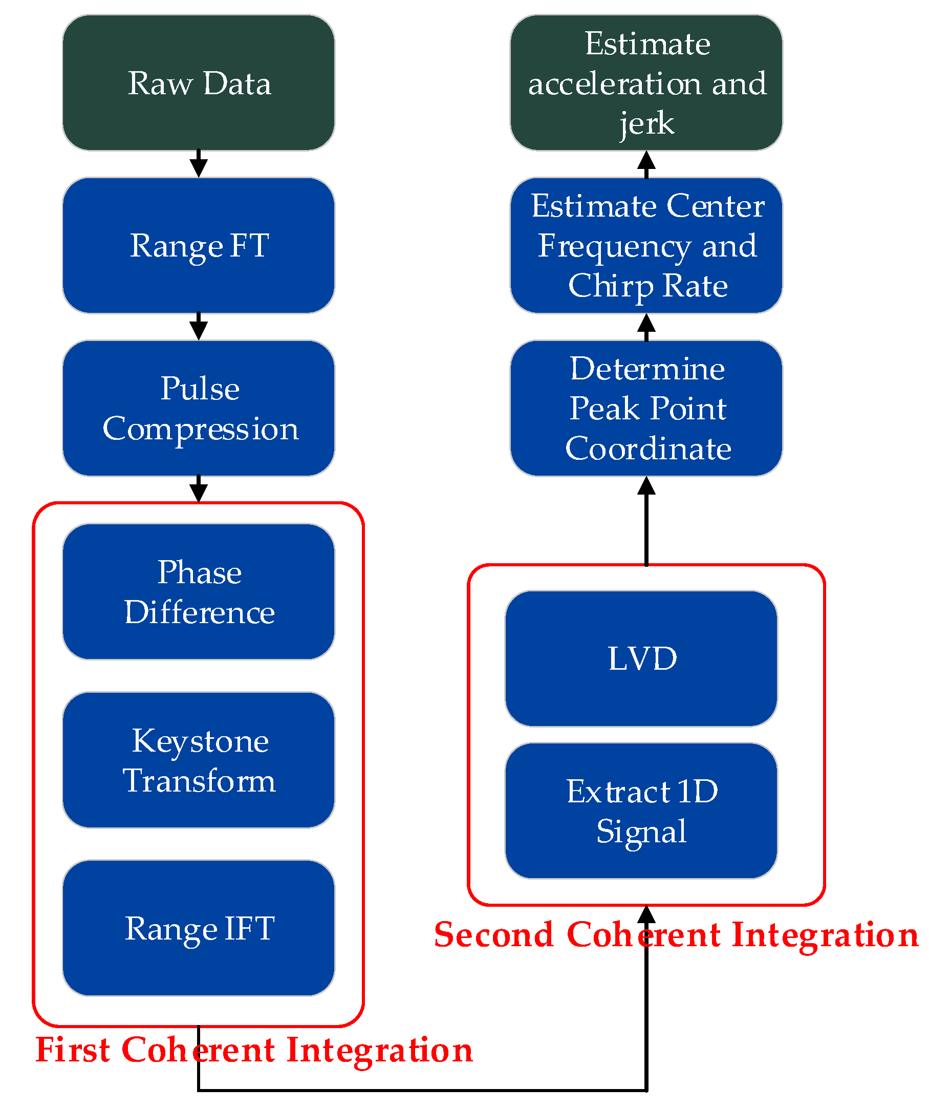
2.2.1. High-Order Polynomial Coefficient Estimation Based on PD-LVD

It is evident that the compressed signal (17) constitutes a multicomponent cubic phase signal at each range frequency $f_r$. Considering the independence of the target’s motion mode from the scatterers’ positions, a PD operation can be employed to integrate signal energy into a single range cell. Simultaneously, the reduction of the Doppler modulation phase’s order and the issue’s simplification are achieved. The following Equation (19) illustrates the PD operation outcome for signal (17) in the range-frequency slow-time domain:

$$\begin{array}{cc}\hfill S_{PD}\left(f_r,t_m;\tau \right)=& S\left(f_r,t_m+\tau \right)S^{*}\left(f_r,t_m-\tau \right)\hfill \\ \hfill =& {\displaystyle \sum _{p=1}^P{\left|{\sigma }_p^{\prime }\right|}^2\exp \left\{-\mathrm{j}4\pi \frac{f_r+f_c}{c}\left[2\tau \left(v+x_p\omega \right)+\frac{1}{3}\beta {\tau }^3+2\alpha \tau t_m+\beta \tau t_m^2\right]\right\}}\hfill \\ & +S_{PDcross-term}\hfill \end{array},$$

(19)

where $\tau$ is the constant lag time variable, $X^{*}$ represents the complex conjugate of $X$, and $S_{PDcross-term}$ are the cross-terms caused by the PD operation. Clearly, the PD operation metamorphoses the cubic phase signal into a chirp signal. For the convenience of observing the integration result, the signal is transformed to the fast-time domain via an IFT concerning the range frequency $f_r$, as shown in (20):

$$\begin{array}{cc}\hfill s_{PD}\left(\widehat{t},t_m;\tau \right)=& {\displaystyle \sum _{p=1}^P{\left|{\sigma }_p^{\prime }\right|}^2\sin \mathrm{c}\left\{B\left[\widehat{t}-\frac{2\left(2\tau \left(v+x_p\omega \right)+\frac{1}{3}\beta {\tau }^3+2\alpha \tau t_m+\beta \tau t_m^2\right)}{c}\right]\right\}}\hfill \\ & \times \exp \left\{-\mathrm{j}4\pi {\displaystyle \frac{f_c}{c}}\left[2\tau \left(v+x_p\omega \right)+{\displaystyle \frac{1}{3}}\beta {\tau }^3+2\alpha \tau t_m+\beta \tau t_m^2\right]\right\}\hfill \\ & +S_{PD-IFTcross-term}\hfill \end{array},$$

(20)

where $S_{PD-IFTcross-term}$ stand for the cross-terms.

From the observation in (20), it is not difficult to find that all of the signal energy is concentrated within range cell $\left(2\tau \left(v+x_p\omega \right)+\beta {\tau }^3/3+2\alpha \tau t_m+\beta \tau t_m^2\right)$, where only $t_m$ is varying over time in the expression. Although $\beta \tau t_m^2$ can be neglected as a high-order term, the linear term $2\alpha \tau t_m$ is large enough that the signal energy will be integrated into different range cells, and against overall SNR gain enhancement. Fortunately, such range migration can be mitigated effectively through the application of KT [39,40]. The virtual slow-time variable $t_n$ is formulated as specified in (21) in accordance with the KT.

$$t_m={\displaystyle \frac{f_c}{f_r+f_c}}{t}_n,$$

(21)

where $t_n$ is the virtual slow-time variable.

Substituting (21) into (19), yields the result of KT as follows:

$$\begin{array}{cc}\hfill S_{PD-KT}\left(f_r,t_n;\tau \right)& ={\displaystyle \sum _{p=1}^P{\left|{\sigma }_p^{\prime }\right|}^2\exp \left\{-\mathrm{j}4\pi \frac{f_r+f_c}{c}\left[2\tau \left(v+x_p\omega \right)+\frac{1}{3}\beta {\tau }^3\right]\right\}}\\ & \times \exp \left\{-\mathrm{j}4\pi {\displaystyle \frac{f_c}{c}}\cdot 2\alpha \tau t_n\right\}\hfill \\ & \times \exp \left\{-\mathrm{j}4\pi {\displaystyle \frac{f_c^2}{c\left(f_r+f_c\right)}}\cdot \beta \tau t_n^2\right\}\hfill \\ & +S_{PD-KTcross-term}\hfill \end{array},$$

(22)

where $S_{PD-KTcross-term}$ represent the cross-terms. One can observe that after applying the KT, the range frequency $f_r$ and the slow-time variable $t_n$ have been decoupled in the first-order coefficient. However, the coupling phenomenon persists in the second-order coefficient despite the application of KT, necessitating crucial approximations and operations. Given that $f_r\ll f_c$, the following approximation is justified according to Taylor expansion:

$${\displaystyle \frac{f_c^2}{f_r+f_c}}\approx \left(1-{\displaystyle \frac{f_r}{f_c}}\right)f_c=f_c-f_r.$$

(23)

Substituting (23) into (22), the KT result can be rewritten as

$$\begin{array}{cc}\hfill S_{PD-KT}\left(f_r,t_n;\tau \right)=& {\displaystyle \sum _{p=1}^P{\left|{\sigma }_p^{\prime }\right|}^2\exp \left\{-\mathrm{j}4\pi \frac{f_r+f_c}{c}\left[2\tau \left(v+x_p\omega \right)+\frac{1}{3}\beta {\tau }^3\right]\right\}}\hfill \\ & \times \exp \left\{-\mathrm{j}4\pi {\displaystyle \frac{f_c}{c}}\cdot 2\alpha \tau t_n\right\}\hfill \\ & \times \exp \left\{-\mathrm{j}4\pi {\displaystyle \frac{f_c-f_r}{c}}\cdot \beta \tau t_n^2\right\}\hfill \\ & +S_{PD-KTcross-term}\hfill \end{array}.$$

(24)

To observe the fast-time domain signal, IFT concerning the range frequency $f_r$ is conducted, obtaining

$$\begin{array}{cc}\hfill s_{PD-KT}\left(\widehat{t},t_n;\tau \right)=& {\displaystyle \sum _{p=1}^P{\left|{\sigma }_p^{\prime }\right|}^2\sin \mathrm{c}\left\{B\left[\widehat{t}-\frac{2\left(2\tau v+2\tau x_p\omega +\frac{1}{3}\beta {\tau }^3-\beta \tau t_n^2\right)}{c}\right]\right\}}\hfill \\ & \times \exp \left\{-\mathrm{j}{\displaystyle \frac{4\pi }{\lambda }}\left[2\tau \left(v+x_p\omega \right)+{\displaystyle \frac{1}{3}}\beta {\tau }^3+2\alpha \tau t_n+\beta \tau t_n^2\right]\right\}\hfill \\ & +s_{PD-KTcross-term}\hfill \end{array},$$

(25)

where $s_{PD-KTcross-term}$ are the cross-terms in the fast-time domain.

From (25), it’s obvious that all of the signal energy is concentrated within range cell $\left(2\tau v+2\tau x_p\omega +\beta {\tau }^3/3-\beta \tau t_n^2\right)$. The monomials $2\tau x_p\omega$ and $\beta \tau t_n^2$ are somewhat small and always negligible in practical scenarios, despite their spatial and temporal variability. In this manner, the range cell of energy concentration can be determined as $\left(2\tau v+\beta {\tau }^3/3\right)$. As for the cross-terms $s_{PD-KTcross-term}$, as detailed in Appendix A, their energy also concentrates within certain range cells, albeit with significantly weaker amplitudes compared to the auto-terms. Therefore, the 2D echo data can be coherently integrated into the 1D signal by extracting the certain range cell with the maximum energy, shown in (26), thereby potentially yielding a significant SNR gain enhancement:

$$\begin{array}{cc}\hfill s\left(t_n\right)& ={\displaystyle \sum _{p=1}^P{A}_p\exp \left\{-\mathrm{j}\frac{4\pi }{\lambda }\left[2\tau \left(v+x_p\omega \right)+\frac{1}{3}\beta {\tau }^3+2\alpha \tau t_n+\beta \tau t_n^2\right]\right\}}\hfill \\ & ={\displaystyle \sum _{p=1}^P{A}_p\exp \left(\mathrm{j}{\phi }_p+\mathrm{j}2\pi f_0{t}_n+\mathrm{j}\pi {\mu }_0{t}_n^2\right)}\hfill \end{array},$$

(26)

where $A_p={\left|{\sigma }_p^{\prime }\right|}^2\sin \mathrm{c}\left[B\left(\widehat{t}-t_0\right)\right]$, $t_0$ is the fast time corresponding to the maximum energy range cell, and ${\phi }_p=-{\displaystyle \frac{4\pi }{\lambda }}\left[2\tau \left(v+x_p\omega \right)\right]$, $f_0=-{\displaystyle \frac{4\alpha \tau }{\lambda }}$, and ${\mu }_0=-{\displaystyle \frac{4\beta \tau }{\lambda }}$ are the initial phases of the pth scatterer, center frequency, and chirp rate, respectively.

As indicated in (26), the extracted range cell manifests as a multicomponent chirp signal, wherein the center frequency and chirp rate denote the parameters of translational motion for the observed target. Supposing that accurate estimations for the chirp signal are acquired, the motion parameters can be determined as follows:

$$\left\{\begin{array}{c}\widehat{\alpha }=-\lambda {\displaystyle \frac{{\widehat{f}}_0}{4\tau }}\hfill \\ \widehat{\beta }=-\lambda {\displaystyle \frac{{\widehat{\mu }}_0}{4\tau }}\hfill \end{array}\right.,$$

(27)

where ${\widehat{f}}_0$ and ${\widehat{\mu }}_0$ represent the estimations of $f_0$ and ${\mu }_0$, respectively.

Now the current issue shifts to the parameter estimation of the chirp signal. Once the signal parameters (center frequency and chirp rate) are accurately estimated, the translational parameters of the target can be precisely inferred, thus enabling the completion of translational compensation. Fortunately, LVD [34], a bilinear time-frequency method that transforms a chirp signal to the center frequency-chirp rate (CFCR) domain, can qualify this issue effectively. One of the pivotal procedures of LVD involves a scaling transformation that ensures its outcomes are devoid of cross-term interference [41]. A comprehensive introduction to LVD will be provided in the subsequent paragraphs.

The parametric symmetric instantaneous auto-correlation function (PSIAF) for the $s\left(t_n\right)$ is denoted as

$$\begin{array}{cc}\hfill R_{\mathrm{PSIAF}}\left(t_n,\widehat{\tau }\right)& =s\left(t_n+{\displaystyle \frac{\widehat{\tau }}{2}}\right)s^{*}\left(t_n-{\displaystyle \frac{\widehat{\tau }}{2}}\right)\hfill \\ & ={\displaystyle \sum _{p=1}^P{A}_p^2\exp \left\{\mathrm{j}2\pi f_0\widehat{\tau }+\mathrm{j}2\pi {\mu }_0{t}_n\widehat{\tau }\right\}}+R_{\mathrm{PSIAF}\mathrm{cross}-\mathrm{term}}\hfill \end{array},$$

(28)

where $\widehat{\tau }$ is a time lag variable and $R_{\mathrm{PSIAF}\mathrm{cross}-\mathrm{term}}$ represent the cross-terms in the PSIAF.

From (28), there is coupling between the time variable $t_n$ and the lag variable $\widehat{\tau }$. This coupling phenomenon can be eliminated by employing a scaling transformation approach, which is inspired by KT. With the help of the construction of a virtual time variable ${\overline{t}}_n=t_n\widehat{\tau }$, the PSIAF can be rewritten as

$${\overline{R}}_{\mathrm{PSIAF}}\left({\overline{t}}_n,\widehat{\tau }\right)={\displaystyle \sum _{p=1}^P{A}_p^2\exp \left\{\mathrm{j}2\pi f_0\widehat{\tau }+\mathrm{j}2\pi {\mu }_0{\overline{t}}_n\right\}}+{\overline{R}}_{\mathrm{PSIAF}-\mathrm{cross}-\mathrm{term}},$$

(29)

where ${\overline{R}}_{\mathrm{PSIAF}}$ and ${\overline{R}}_{\mathrm{PSIAF}-\mathrm{cross}-\mathrm{term}}$ are the PSIAF and cross-terms after the scaling transformation. It is clear that ${\overline{R}}_{\mathrm{PSIAF}}$ has been decoupled and a 2D FT is applied to compute the LVD of $s\left(t_n\right)$, as illustrated in (30).

$$\begin{array}{cc}\hfill \mathrm{LVD}\left\{s\left(t_n\right)\right\}& ={\mathrm{FT}}_{2D}\left\{{\overline{R}}_{\mathrm{PSIAF}}\left({\overline{t}}_n,\widehat{\tau }\right)\right\}\hfill \\ & ={\displaystyle \sum _{p=1}^P{A}_p^2\delta \left(f-f_0\right)\delta \left(\mu -{\mu }_0\right)}+{\mathrm{FT}}_{2D}\left\{{\overline{R}}_{\mathrm{PSIAF}-\mathrm{cross}-\mathrm{term}}\right\}\hfill \end{array},$$

(30)

where $\delta \left(*\right)$ is the Dirac function, and $f$ and $\mu$ are the center frequency variable and chirp rate variable, respectively.

Obviously, the 1D signal is coherently integrated to a peak point in the CFCR plane, and the estimations of the signal’s parameters can be obtained by easily determining the location of the peak. However, it is noteworthy that the cross-terms are still lying in (30). Indeed, prior research by the authors, as cited in [3], has demonstrated that the cross-terms do not coherently integrate after FT, thus exerting a negligible impact on the resulting outcome. This finding leads to the asymptotic linearity of LVD, as shown in (31):

$$\mathrm{LVD}\left\{s\left(t_n\right)\right\}\approx {\displaystyle \sum _{p=1}^P{A}_p^2\delta \left(f-f_0\right)\delta \left(\mu -{\mu }_0\right)}.$$

(31)

Due to this attribute, LVD is a gifted time-frequency method whose performance of robustness and estimation accuracy is awesome.

Since there is both a PD operation and an LVD transformation in the proposed high-order polynomial coefficient estimation method, it is named PD-LVD. According to the descriptions of the proposed method above, Figure 3 presents a specific depiction of PD-LVD to enhance understanding of the entire procedure. After range FT and pulse compression, the first coherent integration is executed to transform all the scatterers’ energy into a certain range cell. One of the most important steps is the PD operation during the first coherent integration, which also contains KT and range IFT. Then the second coherent integration follows, which is composed of signal extraction and LVD. The estimations of signal parameters imply that high-order translational motion coefficients can be derived just by a simple peak point detection.

After two coherent integrations, the energy of the received signal is integrated into a strong peak point by PD-LVD, and the signal parameters’ estimations ${\widehat{f}}_0$ and ${\widehat{\mu }}_0$ are acquired successfully. This allows the construction of the high-order translation compensation function, seen in (32).

$${\mathrm{\Phi }}_{\mathrm{High}-\mathrm{Order}}\left(f_r,t_m\right)=\exp \left\{\mathrm{j}4\pi {\displaystyle \frac{f_r+f_c}{c}}\left({\displaystyle \frac{1}{2}}\widehat{\alpha }{t}_m^2+{\displaystyle \frac{1}{6}}\widehat{\beta }{t}_m^3\right)\right\}.$$

(32)

With the help of the high-order phase compensation function, the negative effects caused by acceleration and jerk will be eliminated heavily:

$$\begin{array}{cc}\hfill S_v\left(f_r,t_m\right)& =S\left(f_r,t_m\right)\times {\mathrm{\Phi }}_{\mathrm{High}-\mathrm{Order}}\left(f_r,t_m\right)\hfill \\ & ={\displaystyle \sum _{p=1}^P{\sigma }_p^{\prime }\exp \left\{-\mathrm{j}4\pi \frac{f_r+f_c}{c}\left[R_0+y_p+\left(x_p\omega +v\right)t_m\right]\right\}}\hfill \end{array}.$$

(33)

2.2.2. First-Order Polynomial Coefficient Estimation Based on ACCA

The PD-LVD processing gives a compensated signal with a linear phase concerning $t_m$ from (33). For a further investigation on the linear phase, $S_v\left(f_r,t_m\right)$ is transformed to the fast-time domain, as (34) presents:

$$\begin{array}{cc}\hfill s_v\left(\widehat{t},t_m\right)=& {\displaystyle \sum _{p=1}^P{\sigma }_p^{\prime }\sin \mathrm{c}\left\{B\left[\widehat{t}-\frac{2\left(R_0+y_p+\left(x_p\omega +v\right)t_m\right)}{c}\right]\right\}}\hfill \\ & \times \exp \left\{-\mathrm{j}4\pi {\displaystyle \frac{f_c}{c}}\left[R_0+y_p+\left(x_p\omega +v\right)t_m\right]\right\}\hfill \end{array}.$$

(34)

Although rotation and translation motions have a similar influence in the linear phase, there is a seriously huge difference in magnitude, in other words, $x_p\omega \ll v$. In such a circumstance, the envelope of the fast-time domain signal can be approximately expressed as

$$\left|s_v\left(\widehat{t},t_m\right)\right|\approx {\displaystyle \sum _{p=1}^P{\sigma }_p^{\prime }\mathrm{sinc}\left\{B\left(\widehat{t}-\frac{2\left(R_0+y_p+v{t}_m\right)}{c}\right)\right\}},$$

(35)

where $\left|X\right|$ represents the modulus of $X$. Looking at the expression, a linear migration in the range profiles is observed due to the velocity, and the displacement between two consecutive envelopes is solely contingent upon the velocity magnitude, implying that the velocity estimation may be generated from the displacement estimation.

As indicated in Section 2, the received data comprises $N$ pulses with a PRI of $\Delta T$, where additionally, $t_m=n\Delta T$ and $n=0,1,2,\cdots ,N-1$. Supposing there are K sample points in a range profile pulse, and the sampling interval is denoted as $\Delta \widehat{t}$, then (35) can be discretized as follows:

$$r_n\left(k\right)={\displaystyle \sum _{p=1}^P{\sigma }_p^{\prime }\mathrm{sinc}\left\{B\left[k\Delta \widehat{t}-\frac{2\left(R_0+y_p+vn\Delta T\right)}{c}\right]\right\}},$$

(36)

where $r_n\left(k\right)$ means the nth pulse’s kth sample point, and $k=0,1,2,\cdots ,K-1$.

Clearly, there is a fixed displacement for arbitrary range profiles $r_{n_1}\left(k\right)$ and $r_{n_2}\left(k\right)$, as (37) demonstrates:

$$r_{n_2}\left(k\right)=r_{n_1}\left(k-k\left(n_2,n_1\right)\right),$$

(37)

where $k\left(n_2,n_1\right)=v\left(n_2-n_1\right)\Delta T/(c/2B)$ represents the displacement of $r_{n_2}\left(k\right)$ relative to $r_{n_1}\left(k\right)$. When we perform a Discrete FT (DFT) on both sides of (37) simultaneously, and the frequency domain expression is shown as

$$R_{n_2}\left(u\right)=R_{n_1}\left(u\right)\exp \left\{-\mathrm{j}{\displaystyle \frac{2\pi }{K}}uk\left(n_2,n_1\right)\right\},$$

(38)

where u is the frequency variable, and $R_{n_1}\left(u\right)$ and $R_{n_2}\left(u\right)$ represent the DFT results of $r_{n_1}\left(k\right)$ and $r_{n_2}\left(k\right)$, respectively. The displacement manifests through the linear phase, which can be acquired via a cross-correlation operation, as (39) shows.

$$S_{CC}\left(u\right)={\displaystyle \frac{R_{n_1}\left(u\right)R_{n_2}^{*}\left(u\right)}{\left|R_{n_1}\left(u\right)R_{n_2}^{*}\left(u\right)\right|}}=\exp \left\{\mathrm{j}{\displaystyle \frac{2\pi }{K}}uk\left(n_2,n_1\right)\right\},$$

(39)

where $S_{CC}\left(u\right)$ represents the cross-correlation function of $R_{n_1}\left(u\right)$ and $R_{n_2}\left(u\right)$, and $u\in \left[-\left(K-1\right),K-1\right]$ is the index variable. The result is normalized since the pertinent information resides only within the phase component.

According to (39), a simple inverse DFT (IDFT) is capable to estimate the displacement $k\left(n_2,n_1\right)$, as shown in

$$s_{CC}\left(k\right)=\mathrm{IDFT}\left\{S_{CC}\left(u\right)\right\}=\delta \left(k-k\left(n_2,n_1\right)\right),$$

(40)

where $s_{CC}\left(k\right)$ is the IDFT result of $S_{CC}\left(u\right)$.

Under ideal conditions, displacement estimation can be successfully derived through peak detection simply. Unfortunately, this method is seriously affected by the noise and clutter inevitable in the realistic complex electromagnetic environment. Furthermore, it can only offer a solution with an accuracy limited to one range resolution for the reason of discretization, leading to terrible performance. The following offers a comprehensive introduction to ACCA, a method adept at effectively addressing these issues.

Consider that the frequency spectrum of the range profiles is affected by zero mean additive Gaussian noise, which has a constant variance, as illustrated in (41).

$$\left\{\begin{array}{c}{\widehat{R}}_{n_1}\left(u\right)=R_{n_1}\left(u\right)\exp \left\{\mathrm{j}{\eta }_{n_1}\left(u\right)\right\}\hfill \\ {\widehat{R}}_{n_2}\left(u\right)=R_{n_2}\left(u\right)\exp \left\{\mathrm{j}{\eta }_{n_2}\left(u\right)\right\}\hfill \end{array}\right.,$$

(41)

where ${\widehat{R}}_{n_1}\left(u\right)$ and ${\widehat{R}}_{n_2}\left(u\right)$ represent the DFT results with noise, and ${\eta }_{n_1}\left(u\right)$ and ${\eta }_{n_2}\left(u\right)$ are the phase noise that is assumed to be independent and identically distributed. In this way, the cross-correlation function (CCF) of ${\widehat{R}}_{n_1}\left(u\right)$ and ${\widehat{R}}_{n_2}\left(u\right)$ can be written as

$${\widehat{S}}_{CC}\left(u\right)=S_{CC}\left(u\right)\exp \left\{\mathrm{j}{\eta }_S\left(u\right)\right\},$$

(42)

where ${\widehat{S}}_{CC}\left(u\right)$ is the CCF with noise and ${\eta }_S\left(u\right)={\eta }_{n_1}\left(u\right)-{\eta }_{n_2}\left(u\right)$ is the phase noise. The aforementioned IDFT method employs ${\widehat{S}}_{CC}\left(u\right)$ for estimation instead of $S_{CC}\left(u\right)$, which contributes to its poor performance.

The auto-cross-correlation function (ACCF) of ${\widehat{R}}_{n_1}\left(u\right)$ and ${\widehat{R}}_{n_2}\left(u\right)$ in this paper is defined as

$$\begin{array}{cc}\hfill S_{ACC}\left(\xi \right)& ={\displaystyle \frac{1}{C\left(\xi \right)}}{\displaystyle \sum _u{\widehat{S}}_{CC}\left(u\right){\widehat{S}}_{CC}^{*}\left(u-\xi \right)}\hfill \\ & ={\displaystyle \frac{1}{C\left(\xi \right)}}{S}_{CC}\left(\xi \right){\displaystyle \sum _u\exp \left\{\mathrm{j}{\eta }_S\left(u\right)-\mathrm{j}{\eta }_S\left(u-\xi \right)\right\}}\hfill \end{array},$$

(43)

where $C\left(\xi \right)$ is the number of sum terms, and $\xi \in \left[-\left(2K-2\right),2K-2\right]$ is the index variable. Significantly, the ACCF $S_{ACC}\left(\xi \right)$ represents the auto-correlation function of CCF ${\widehat{S}}_{CC}\left(u\right)$ from (43), and that’s why it’s named ACCF. Appendix B demonstrates that the expectation of $S_{ACC}\left(\xi \right)$ shares the same phase as the idea of noise-free CCF $S_{CC}\left(\xi \right)$, while additionally exhibiting superior noise variance performance compared to CCF ${\widehat{S}}_{CC}\left(\xi \right)$, making ACCF a preferable alternative for estimating. The remainder of this section introduces the proposed method for estimating displacement (velocity) using ACCF, referred to as the auto-cross-correlation algorithm (ACCA).

The ACCF can be rewritten as

$$S_{ACC}\left(\xi \right)=\exp \left\{\mathrm{j}{\displaystyle \frac{2\pi }{K}}\xi k\left(n_2,n_1\right)\right\}\cdot N_{ACC}\left(\xi \right),$$

(44)

where $N_{ACC}\left(\xi \right)={\displaystyle \sum _u\exp \left\{\mathrm{j}{\eta }_S\left(u\right)-\mathrm{j}{\eta }_S\left(u-\xi \right)\right\}}/C\left(\xi \right)$ represents the phase noise. It is worth noting that not all elements in the $S_{ACC}\left(\xi \right)$ sequence are employed in reality. To ensure robustness and accuracy, only elements incorporating a significantly greater number of summation terms prove beneficial. This assumes that Q elements are selected to be treated by the proposed method, which can be expressed as

$${\mathit{s}}_Q={\left(S_{ACC}\left({\xi }_1\right),S_{ACC}\left({\xi }_2\right),S_{ACC}\left({\xi }_3\right),\cdots ,S_{ACC}\left({\xi }_Q\right)\right)}^{\mathrm{T}},$$

(45)

where ${\mathit{s}}_Q$ is the selected vector, and $\left({\xi }_1,{\xi }_2,{\xi }_3,\cdots ,{\xi }_Q\right)$ correspond to the indexes of elements that have the first Q large sum terms.

Let

$${\mathit{w}}_Q={\left(\exp \left\{\mathrm{j}{w}_{1}k\left(n_2,n_1\right)\right\},\exp \left\{\mathrm{j}{w}_{2}k\left(n_2,n_1\right)\right\},\cdots ,\exp \left\{\mathrm{j}{w}_{Q}k\left(n_2,n_1\right)\right\}\right)}^{\mathrm{T}},$$

(46)

where $w_q=2\pi {\xi }_q/K$. Then the displacement estimation problem can be regarded as an unconstrained global optimization, as shown in

$$〈\widehat{k}\left(n_2,n_1\right)〉=\arg \underset{k\left(n_2,n_1\right)}{\min }{‖{\mathit{s}}_Q-{\mathit{w}}_Q‖}_2^2,$$

(47)

where $\widehat{k}\left(n_2,n_1\right)$ is the estimation of the displacement. Thanks to the fact that the valuable information only lies in the phase component, the optimization model can be reformulated into a phase representation as

$$〈\widehat{k}\left(n_2,n_1\right)〉=\arg \underset{k\left(n_2,n_1\right)}{\min }{‖\mathrm{Phase}\left\{s_Q\right\}-\mathrm{Phase}\left\{w_Q\right\}‖}_2^2,$$

(48)

where $\mathrm{Phase}\left\{X\right\}$ means the phase of $X$, and $\mathrm{Phase}\left\{w_Q\right\}=k\left(n_2,n_1\right){\left(w_1,w_2,\cdots ,w_Q\right)}^{\mathrm{T}}$. Let $\psi =\mathrm{Phase}\left\{s_Q\right\}$ and $w={\left(w_1,w_2,\cdots ,w_Q\right)}^{\mathrm{T}}$, then (48) can be rewritten as

$$〈\widehat{k}\left(n_2,n_1\right)〉=\arg \underset{k\left(n_2,n_1\right)}{\min }{‖\psi -k\left(n_2,n_1\right)w‖}_2^2,$$

(49)

where $k\left(n_2,n_1\right)$ is an unknown parameter to be determined, $w$ represents an artificially constructed vector, and $\psi$ can be computed from the received signal. The LS solution of this optimization is derived as

$$\widehat{k}\left(n_2,n_1\right)={\left(w^{\mathrm{T}}w\right)}^{-1}{w}^{\mathrm{T}}\psi .$$

(50)

The estimation of displacement between any two arbitrary range profiles can be obtained by leveraging Equation (50). Thanks to the LS solution, the optimization-based method achieves a more accurate sub-resolution solution without escalating the computational load. Selecting the initial range profile as the reference, the displacement vector $\mathbf{\Delta }k$ can be generated, as illustrated in

$$\mathbf{\Delta }k={\left(\widehat{k}\left(1,1\right),\widehat{k}\left(2,1\right),\widehat{k}\left(3,1\right),\cdots ,\widehat{k}\left(N,1\right)\right)}^{\mathrm{T}}.$$

(51)

Correspondingly, the slow time vector $\mathbf{\Delta }t$ is constructed as

$$\mathbf{\Delta }t={\left(0,\Delta T,2\Delta T,\cdots ,\left(N-1\right)\Delta T\right)}^{\mathrm{T}}.$$

(52)

If the high-order translational motion is compensated ideally, the relationship as (53) shows holds.

$$\left\{\left(\Delta t_i,\Delta k_i\right)\left|i=1,2,3,\cdots ,N\right.\right\}\subseteq \left\{\left(x,y\right)\left|y=vx, x\in ℝ\right.\right\},$$

(53)

where $\Delta t_i$ and $\Delta k_i$ are the ith element in $\mathbf{\Delta }t$ and $\mathbf{\Delta }k$, respectively. These point pairs $\left(\Delta t_i,\Delta k_i\right)$ lie on a line passing through the origin, with its slope exactly representing the velocity $v$. In other words, the velocity estimation $\widehat{v}$ can be derived from the slope of this line. Based on $\mathbf{\Delta }k$ and $\mathbf{\Delta }t$, the slope vector $\mathit{\gamma }$ is written as

$$\gamma ={\left({\displaystyle \frac{\widehat{k}\left(2,1\right)}{\Delta T}},{\displaystyle \frac{\widehat{k}\left(3,1\right)}{2\Delta T}},\cdots ,{\displaystyle \frac{\widehat{k}\left(N,1\right)}{\left(N-1\right)\Delta T}}\right)}^{\mathrm{T}}.$$

(54)

Under ideal conditions, all elements in $\gamma$ are very similar. Therefore, the estimation of the line’s slope can be obtained simply by computing the average of the slope vectors. However, the observed slope values always fluctuate seriously around the true value due to the influence of noise and clutter. To address this issue, the slope histogram is introduced to select more meaningful data points during estimation.

Assuming there are L levels in the histogram, the range of each bin is then

$$\Delta ={\displaystyle \frac{\max \left(\gamma \right)-\min \left(\gamma \right)}{L}},$$

(55)

where $\max \left(X\right)$ and $\min \left(X\right)$ represent the maximum and minimum of $X$, respectively. As a result, L bins $\left[\min \left(\gamma \right),\min \left(\gamma \right)+\Delta \right)$, $\left[\min \left(\gamma \right)+\Delta ,\min \left(\gamma \right)+2\Delta \right)$, …, $\left[\min \left(\gamma \right)+\left(L-1\right)\Delta ,\min \left(\gamma \right)+L\Delta \right]$ emerge. The slope histogram $H_{\gamma }$ can then be established by allocating all the elements in $\gamma$ into these L bins. Finally, the bin with the highest frequency of data points is utilized for velocity estimation, as shown in

$$\widehat{v}={\displaystyle \frac{{\displaystyle \sum \gamma \left(I_{pick}\right)}}{\mathrm{length}\left(I_{pick}\right)}},$$

(56)

where $I_{pick}$ and $\mathrm{length}\left(I_{pick}\right)$ represent the indexes and number of the picked data points, respectively. The proposed method raises the amount of accuracy and robustness by screening out those data points that are unacceptable. For a specific and detailed demonstration, Algorithm 1 gives a complete pseudocode of ACCA.

Algorithm 1: Auto-Cross-Correlation Algorithm (ACCA)

Input: The discrete range profiles: $\left\{r_n\left(k\right)\left|n=0,1,2,\cdots ,N-1;k=0,1,2,\cdots ,K-1\right.\right\}$. Output: The estimation of the first-order translational motion parameter: $\widehat{v}$. 1: Use DFT to transform the signal to frequency domain. ${\widehat{R}}_n\left(u\right)\leftarrow \mathrm{DFT}\left\{r_n\left(k\right)\right\}$; 2: For Iterate over the slow time indexes $n\leftarrow 0,1,\dots ,N-1$; 3:  Calculate the CCF ${\widehat{S}}_{CC}\left(u\right)\leftarrow {\displaystyle \frac{{\widehat{R}}_0\left(u\right){\widehat{R}}_n^{*}\left(u\right)}{\left|{\widehat{R}}_0\left(u\right){\widehat{R}}_n^{*}\left(u\right)\right|}}$; 4:  Calculate the ACCF $S_{ACC}\left(\xi \right)\leftarrow {\displaystyle \frac{1}{C\left(\xi \right)}}{\displaystyle \sum _u{\widehat{S}}_{CC}\left(u\right){\widehat{S}}_{CC}^{*}\left(u-\xi \right)}$; 5:  Select Q data points in the middle of ACCF to construct $s_Q$, $s_Q\leftarrow {\left(S_{ACC}\left({\xi }_1\right),S_{ACC}\left({\xi }_2\right),S_{ACC}\left({\xi }_3\right),\cdots ,S_{ACC}\left({\xi }_Q\right)\right)}^{\mathrm{T}}$; 6:  Compute the phase vector $\psi \leftarrow \mathrm{Phase}\left\{s_Q\right\}$; 7:  Construct vector $w\leftarrow {\left(w_1,w_2,\cdots ,w_Q\right)}^{\mathrm{T}}$; 8:  Estimate the displacement $\widehat{k}\left(n+1,1\right)\leftarrow {\left(w^{\mathrm{T}}w\right)}^{-1}{w}^{\mathrm{T}}\psi$; 9: End For 10: Construct the displacement vector $\mathbf{\Delta }k\leftarrow {\left(\widehat{k}\left(1,1\right),\widehat{k}\left(2,1\right),\cdots ,\widehat{k}\left(N,1\right)\right)}^{\mathrm{T}}$; 11: Construct the slow time vector $\mathbf{\Delta }t\leftarrow {\left(0,\Delta T,\cdots ,\left(N-1\right)\Delta T\right)}^{\mathrm{T}}$; 12: Calculate the slope vector $\gamma ={\left({\displaystyle \frac{\widehat{k}\left(2,1\right)}{\Delta T}},{\displaystyle \frac{\widehat{k}\left(3,1\right)}{2\Delta T}},\cdots ,{\displaystyle \frac{\widehat{k}\left(N,1\right)}{\left(N-1\right)\Delta T}}\right)}^{\mathrm{T}}$; 13: Establish the slope histogram $H_{\gamma }$; 14: Detect the bin with the most points and save the picked indexes $I_{pick}\leftarrow \mathrm{Find}\_\mathrm{Max}\_\mathrm{Bin}\left(H_{\gamma }\right)$; 15: Estimate the first-order translational motion parameter $\widehat{v}\leftarrow {\displaystyle \frac{{\displaystyle \sum \gamma \left(I_{pick}\right)}}{\mathrm{length}\left(I_{pick}\right)}}$;

Once the velocity estimation has been obtained, the first-order translation compensation function is subsequently constructed, denoted as

$${\mathrm{\Phi }}_{\mathrm{First}-\mathrm{Order}}\left(f_r,t_m\right)=\exp \left\{\mathrm{j}4\pi {\displaystyle \frac{f_r+f_c}{c}}v{t}_m\right\}.$$

(57)

Then, the remaining first-order translational motion can be fully compensated by applying the compensation function to the signal (33), which is free of high-order motion parameters. The compensation process is illustrated as

$$\begin{array}{cc}\hfill S_{\mathrm{TMC}}\left(f_r,t_m\right)& =S_v\left(f_r,t_m\right)\times {\mathrm{\Phi }}_{\mathrm{First}-\mathrm{Order}}\left(f_r,t_m\right)\hfill \\ & ={\displaystyle \sum _{p=1}^P{\sigma }_p^{\prime }\exp \left\{-\mathrm{j}4\pi \frac{f_r+f_c}{c}\left[R_0+y_p+x_p\omega t_m\right]\right\}}\hfill \end{array},$$

(58)

where $S_{\mathrm{TMC}}\left(f_r,t_m\right)$ is the signal after translational motion compensation. From (58), all the translational motion parameters are eliminated thoroughly. It gives a guarantee of a well-focused ISAR image following compensation, as (14) shows.

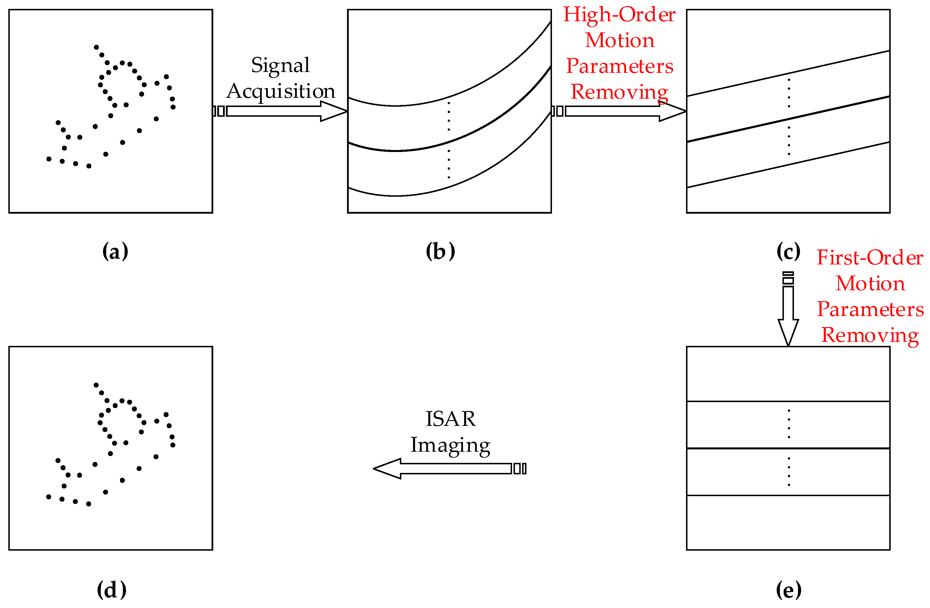
2.2.3. Translational Motion Compensation and ISAR Imaging Based on the Proposed Method

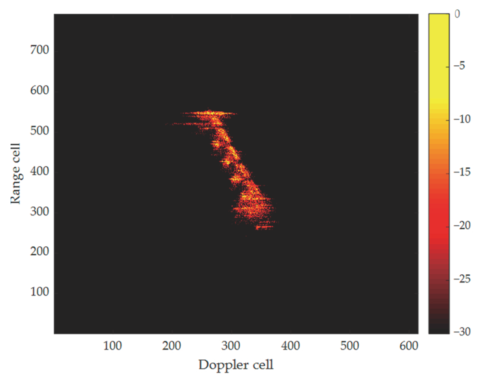
Ultimately, it is observed that all translational motion parameters are accurately estimated, thereby negating the adverse effects caused by the target’s motion, including both the envelope and phase. Figure 4 illustrates the comprehensive procedures of the proposed method as detailed in Section 3, aimed at enhancing understanding. As evident, the entire process is divided into two primary modules: high-order and first-order motion compensations. The high-order motion compensation initiates the process, utilizing the PD-LVD operation to generate estimates of acceleration and jerk, which are crucial for constructing the high-order compensation function. After the first compensation, the high-order motion’s dreadful influence is eliminated, resulting in a linear phase. Then the first-order motion compensation is on the stage. It employs ACCA to estimate the velocity, which plays an important role in the first-order compensation function. After the second compensation, all negative effects of translational motion are fully compensated, yielding a well-focused ISAR image that can be generated using FT and IFT.

3. Results

In this section, extensive experiments are conducted on a measured dataset from a vessel to verify and evaluate the performance of the proposed method for ISAR imaging. The employed vessel data is captured via an X-band ISAR system, with additional parameters detailed in

Table 1. ISAR system parameters for the employed vessel data.

Parameters	Values
Carrier frequency	9.6 GHz
Signal bandwidth	500 MHz
Pulse repetition frequency	125 Hz
Rang samples	792
Azimuth samples	615

. It transmits chirp signals, and the received signals are de-chirped following I/Q sampling. To validate the robustness, the measured data is employed to generate synthetic data at varying SNRs.

To begin, Figure 5 presents the ideal depiction of the illuminated vessel as a reference image. As can be observed, the vessel belongs to a freighter approximately 100 m in length, with the bow positioned at the top of the pattern.

To illustrate the efficacy of the proposed approach, third-order translational motion is introduced into the dataset with an input SNR set to 5 dB. More specifically, the vessel is regarded as having a translational motion with $v=5.0 \mathrm{m}/\mathrm{s}$, $\alpha =3.0 {\mathrm{m}/\mathrm{s}}^2$, and $\beta =0.7 {\mathrm{m}/\mathrm{s}}^3$, yielding a nonlinear range migration and phase error, as Figure 6a shows. Figure 6b gives the ISAR imaging result based on Figure 6a. Apparently, due to significant range migration, the imaging process has failed, and the result is absolutely unacceptable.

It becomes obvious that the nonlinear bending emerges due to the target’s non-stationary motion. Subsequently, the data incorporating translational motion is processed using the PD-LVD method to estimate and compensate for the high-order motion, and the results for each step are illustrated in Figure 7. Figure 7a depicts the outcome post-PD, revealing that the energy from all scatterers is concentrated within two range cells (396# to 398# range cells). To adjust the misalignment, KT is necessary, and Figure 7b illustrates how KT causes the energy to focus on a single range cell (398# range cell). According to the proposed PD-LVD method, the 398# range cell is then extracted as the input for the subsequent LVD process. Figure 7c gives the results of LVD. Apparently, the energy converges to a peak due to the twice coherent integration process. From the results the estimations of acceleration and jerk are 3.0047 ${\mathrm{m}/\mathrm{s}}^2$ and 0.6965 ${\mathrm{m}/\mathrm{s}}^3$, which coincide exactly with the presets. With the aid of estimations, the high-order compensation function is successfully constructed. As depicted in Figure 7d, the high-order compensation effectively eliminates nonlinear bending in the range profiles, leading to linear migration, where only the first-order motion parameter (velocity) introduces negative effects.

ACCA is performed to compensate for the first-order parameters, and Figure 8 presents the results during the processing. Figure 8a shows the displacement estimation results for each range profile relative to the first one. The estimated results suggest a consistent upward trend with a linear characteristic. However, due to the glitter effect and the presence of noise, clutter, and other interference factors, the estimation results fluctuate drastically, complicating the acquisition of target velocity information through displacement estimation values. To ensure accuracy, the slope histogram is generated from the displacement curve, as depicted in Figure 8b. The fact that 72 points fall into the bin whose boundaries are 0.1293 and 0.1402 is plain to see. Based on the proposed algorithm, the mean of these 72 samples is calculated to be 0.1333. When converted to velocity units, it corresponds to 4.9951 m/s, which is consistent with the predefined velocity value. Following the first-order compensation function utilizing the estimated velocity to further correct the range profiles, the outcomes are illustrated in Figure 8c. The range profiles appear flat, indicating successful cancellation of all negative effects of the translational motion. The ISAR imaging result following translational motion compensation through the proposed method is shown in Figure 8d, aligning consistently with Figure 5. A sequence of experiments has demonstrated the method’s effective capability in achieving translational compensation for maneuvering targets.

To validate the remarkable robustness of the proposed approach based on PD-LVD and ACCA, extensive experiments are delivered under different SNRs of 0, −5, and −10 dB. Moreover, the results are exhibited for comparison with the MCRA+PGA method and the IQEM-PSO method in Figure 9. The first row of Figure 9 provides the ideal ISAR images under different SNRs as references. The second row shows the imaging results of the MCRA+PGA method under different SNRs. It can be concluded that the image quality of this method is significantly poor, with performance deteriorating sharply as the SNR decreases from Figure 9d–f. As depicted in the figures, the results of the MCRA+PGA method show pronounced defocusing at 0 dB and inadequate compensation under the conditions of −5 dB and −10 dB. This suggests that achieving satisfactory results with this method for translational motion compensation in low SNR environments is challenging due to the destruction of the coherent characteristics of adjacent pulse. Instead, the IQEM-PSO method demonstrates superior performance compared to the MCRA+PGA method, as Figure 9g–i shows. It can achieve passable compensation under various SNR conditions, albeit in a manner where the defocusing intensifies as the SNR decreases. Particularly, the image obtained via this approach merely presents an approximate representation of the ship at −10 dB, as depicted in Figure 9i, given that the IQEM-PSO algorithm has a propensity to converge towards locally optimal solutions in low SNR environments. In contrast, the results generated from the proposed method are well-focused and similar to ideal results at any SNR condition, as demonstrated in Figure 9j–l. Owing to the 2D coherent integration and the application of ACCF, the proposed method can accurately estimate and compensate for translational parameters and output a clear ISAR image even if SNR = −10 dB. The experimental results reveal that the proposed method demonstrates good stability in low SNR environments and outperforms alternative methods for image quality.

To further assess the efficacy of the proposed method, the repeated experiment is conducted with different motion parameters, which are $v=0.5 \mathrm{m}/\mathrm{s}$, $\alpha =-0.2 {\mathrm{m}/\mathrm{s}}^2$, and $\beta =0.1 {\mathrm{m}/\mathrm{s}}^3$. The misaligned range profiles with translational motion are given in Figure 10a. It appears to be aligned when observed visually due to the small values of the set parameters. However, the negative effects of phase errors for ISAR imaging are detrimental, and Figure 10b convincingly illustrates this perspective. Due to the translational motion of the target, there is a serious smearing effect in the imaging result, and the energy of the scatterers is poorly concentrated. Generally, such imaging results are deemed unacceptable. Applying the proposed method to process the data yields the following estimations: $\widehat{v}=0.4997 \mathrm{m}/\mathrm{s}$, $\widehat{\alpha }=-0.2003 {\mathrm{m}/\mathrm{s}}^2$, and $\widehat{\beta }=0.0998 {\mathrm{m}/\mathrm{s}}^3$. The range profiles following motion compensation are depicted in Figure 10c. Benefiting from accurate estimation results, compensation processing ensures that both the envelope and phase are appropriately corrected, resulting in a well-focused ISAR image, as illustrated in Figure 10d. In comparison to the original image, the structural details of the vessel are significantly clearer, and there is a marked enhancement in image quality. This improvement will facilitate subsequent image interpretation tasks.

Finally, to validate the universality of the proposed method, a dataset of a measured vessel with unknown actual motion parameters was utilized for analysis. Figure 11a,b illustrate the original range profiles and ISAR images of the data, respectively. Figure 11a exhibits not only range migration but also a noticeable level of noise. As a consequence, Figure 11b displays blurring and energy leakage, resulting in a low-quality ISAR image. Using the proposed method, the estimated motion parameters are $\widehat{v}=0.3101 \mathrm{m}/\mathrm{s}$, $\widehat{\alpha }=-0.6328 {\mathrm{m}/\mathrm{s}}^2$, and $\widehat{\beta }=-0.4219 {\mathrm{m}/\mathrm{s}}^3$. Based on the estimations, the precise phase compensation function is formulated, and Figure 11c demonstrates the compensated range profiles. Owing to the strong robustness, almost all the motion effects are eliminated, and the range profiles become straight lines. Figure 11d presents the final imaging result treated by the proposed method. Compared to Figure 11b, there is a notable enhancement in both the degree of focus and the reduction of energy leakage. This result underscores the effectiveness and reliability of the proposed method.

4. Discussion

To quantitatively compare the performance of different methods, image entropy is utilized as an objective criterion for evaluating image quality. Generally, the smaller the entropy at the same SNR, the better the image quality. The image entropy E of an ISAR image $I\left(m,n\right)$ is defined as

$$E={\displaystyle \sum _{m=1}^M{\displaystyle \sum _{n=1}^N\frac{{\left|I\left(m,n\right)\right|}^2}{{\displaystyle \sum _{m=1}^M{\displaystyle \sum _{n=1}^N{\left|I\left(m,n\right)\right|}^2}}}}}\ln {\displaystyle \frac{{\displaystyle \sum _{m=1}^M{\displaystyle \sum _{n=1}^N{\left|I\left(m,n\right)\right|}^2}}}{{\left|I\left(m,n\right)\right|}^2}},$$

(59)

where M and N are the numbers of samples for fast and slow time domains, respectively. After calculating the image entropy of all the ISAR images in Figure 9, the results are summarized in Figure 12.

As you can see, the entropy of the images obtained by the proposed images is the least, yielding the best image quality. The results of the MCRA+PGA method are the worst due to the anti-noise performance being the poorest. Once the SNR is not adequate, the MCRA method will break down. The entropy of the IQEM-PSO method surpasses that of the MCRA+PGA method due to its moderate noise tolerance. Nonetheless, it remains constrained by the issue of local optimal solutions.

To further substantiate the superiority of the proposed method, a comprehensive analysis of the algorithm’s time complexity and SNR gain will be presented in the following.

The time complexity of ACCA is theoretically evaluated and compared with that of MCRA and IQEM-PSO. According to [20], the time complexity of MCRA is

$$C_{MCRA}=O\left(4NK\log K+NK\log N+2NK\right).$$

(60)

As for IQEM-PSO method, its time complexity can be expressed as [33]

$$C_{IQEM-PSO}=O\left(P_{\mathrm{final}}{I}_{\mathrm{partical}}{e}_{\max }NK\left(\log N+\log K\right)+NK\log K+{\displaystyle \sum _{P=1}^{P_{\mathrm{final}}}N{P}^2}\right),$$

(61)

where $P_{\mathrm{final}}$ is the final estimated polynomial order, $I_{\mathrm{partical}}$ is the number of particles, and $e_{\max }$ is the maximum number of iterations. Owing to the search procedure inherent in this method, its computational burden exhibits a high sensitivity to the number of particles and iterations.

The time complexity of ACCA can be inferred from the pseudocode presented in Algorithm 1. ACCA consists of the following procedures: N times K-point FFT, N cross-correlation operations (signal length is K), N auto-correlation operations (signal length is 2K − 1), NK comparisons, N calculate phase operations for a Q-point vector, N assignments for a Q-point vector, N times LS, and L comparisons. Finally, the total computation load is written as

$$C_{ACCA}=O\left(2NK\log K+N\left(2K-1\right)\log \left(2K-1\right)+NK+3NQ+L\right).$$

(62)

When K is relatively large, $N\left(2K-1\right)\log \left(2K-1\right)$ and $2NK\log K$ become similar in value. Furthermore, Q is smaller than K; for instance, Q could be K/4. Additionally, L is significantly smaller than both N and K. Thus, $C_{ACCA}$ can be approximated as

$$C_{ACCA}\approx O\left(4NK\log K+{\displaystyle \frac{7}{4}}NK\right).$$

(63)

Based on the above analysis, it can be inferred that the computational burden of ACCA is the least, particularly when considering the interpolation requirements for MCRA in practical scenarios. The computational burden of IEQM-PSO is the heaviest due to its multi-dimensional search procedure, which hampers its suitability for real-time applications.

A detailed analysis of the SNR gain was subsequently conducted. Assuming the energy of the noise is $E_n$, the input SNR can be written as ${\mathrm{SNR}}_{in}={\displaystyle \sum _{p=1}^P{\sigma }_p^2}/E_n$. As we all know, during range compression, the signal amplitude transforms to $\sqrt{BT}{\sigma }_p$, where $BT=B\times T_p$ represents the time–bandwidth product. Based on this information, the output SNR after range compression is ${\mathrm{SNR}}_{RC}={\displaystyle \sum _{p=1}^P{\left(\sqrt{BT}{\sigma }_p\right)}^2}/E_n=BT {\mathrm{SNR}}_{in}$. After the application of PD and KT, the energy is coherently concentrated within a single range cell. The energy contained within this range cell is ${\displaystyle \sum _{p=1}^P{\left(BT{\sigma }_p^2\right)}^2}$, while the noise energy present in the same range cell is represented as $E_n^2/K$. Therefore, the output SNR after PD-KT is ${\mathrm{SNR}}_{PD-KT}={\displaystyle \sum _{p=1}^P{\left(BT{\sigma }_p^2\right)}^2}/E_n^2/K=K {\mathrm{SNR}}_{RC}^2$. Finally, LVD is utilized to achieve coherent integration, thereby concentrating the energy into a prominent peak, and the output SNR after LVD is ${\mathrm{SNR}}_{PD-KT-LVD}=N {\mathrm{SNR}}_{PD-KT}$. Hence, the relationship between ${\mathrm{SNR}}_{in}$ and ${\mathrm{SNR}}_{out}$ can be elucidated as ${\mathrm{SNR}}_{out}=NKB{T}^2{\mathrm{SNR}}_{in}^2$, and the decibel (dB) representation is as follows:

$${\mathrm{SNR}}_{out}=2{\mathrm{SNR}}_{in}+10\log N+10\log K+20\log BT.$$

(64)

For the IQEM-PSO method, which utilizes 2D-coherent integration of range and azimuth compressions, the relationship between the input SNR and output SNR can be expressed as ${\mathrm{SNR}}_{out}^{\prime }=NK{\mathrm{SNR}}_{in}$. The dB representation, similarly, is written as

$${\mathrm{SNR}}_{out}^{\prime }={\mathrm{SNR}}_{in}+10\log N+10\log K,$$

(65)

where ${\mathrm{SNR}}_{out}^{\prime }$ means the output SNR with IQEM-PSO method.

Based on (64) and (65), it is evident that the proposed method significantly enhances the output SNR. It incorporates two coherent integrations, concentrating the entire energy into a prominent peak, thereby facilitating exceptional noise immunity. Overall, the proposed method demonstrates exceptional resilience to noise and holds considerable promise for producing high-quality ISAR images in practice.

5. Conclusions

This paper focuses on the translational motion compensation for a non-stationary moving target during ISAR imaging. Although extensive methods have been proposed to address the issue, they typically struggle to perform well in scenarios with low SNR. With this background, a robust method based on PD-LVD and ACCA is developed in this paper. With the assistance of the third-order motion model of the target, the PD-LVD technique can focus all target energy onto a strong point, significantly enhancing the SNR gain. With the help of the definition of ACCF, the ACCA method is developed to estimate the first-order polynomial coefficient. The proposed ACCA method exhibits superior noise tolerance compared to traditional approaches and is capable of achieving a sub-resolution solution without the need for exhaustive searching, thereby ensuring both robustness and efficiency. Finally, the experimental results demonstrate that the proposed method achieves outstanding imaging performance with superior image quality compared to state-of-the-art approaches.

References

1. Ozdemir, C. Inverse Synthetic Aperture Radar Imaging with MATLAB Algorithms, 2nd ed.; John Wiley and Sons, Inc.: Hoboken, NJ, USA, 2021. [Google Scholar]
2. Cumming, I.G.; Wong, F.H. Digital Processing of Synthetic Aperture Radar Data Algorithms and Implementation; Artech House Publishers: Norwood, MA, USA, 2005. [Google Scholar]
3. Liu, C.; Luo, Y.; Yu, Z.; Feng, J. ISAR Imaging of Non-Stationary Moving Target Based on Parameter Estimation and Sparse Decomposition. Remote Sens. 2023, 15, 22. [Google Scholar] [CrossRef]
4. Xiong, S.; Li, K.; Wang, H.; Zhao, S.; Luo, Y.; Zhang, Q. Sparse Aperture High-Resolution RID ISAR Imaging of Maneuvering Target Based on Parametric Efficient Sparse Bayesian Learning. IEEE Geosci. Remote Sens. Lett. 2024, 21, 5. [Google Scholar] [CrossRef]
5. Liu, W.; Wang, H.; Yang, Q.; Deng, B.; Fan, L.; Yi, J. High Precision Motion Compensation THz-ISAR Imaging Algorithm Based on KT and ME-MN. Remote Sens. 2023, 15, 22. [Google Scholar] [CrossRef]
6. Li, D.; Zhan, M.; Liu, H.; Liao, Y.; Liao, G. A Robust Translational Motion Compensation Method for ISAR Imaging Based on Keystone Transform and Fractional Fourier Transform under Low SNR Environment. IEEE Trans. Aerosp. Electron. Syst. 2017, 53, 2140–2156. [Google Scholar] [CrossRef]
7. Jack, L.W. Range-Doppler Imaging of Rotating Objects. IEEE Trans. Aerosp. Electron. Syst. 1980, 1, 23–52. [Google Scholar]
8. Zhang, Z.; Zhang, L.; Wu, J.; Guo, W. Optical and Synthetic Aperture Radar Image Fusion for Ship Detection and Recognition: Current state, challenges, and future prospects. IEEE Geosci. Remote Sens. Mag. 2024, 2–38. [Google Scholar] [CrossRef]
9. Chen, J.; Wu, Y.; Gao, X.; Dai, W.; Zeng, X.; Diao, W.; Sun, X. DPFF-Net: Dual-Polarization Image Feature Fusion Network for SAR Ship Detection. IEEE Trans. Geosci. Remote Sens. 2023, 61, 5216514. [Google Scholar] [CrossRef]
10. Wang, C.; Pei, J.; Luo, S.; Huo, W.; Huang, Y.; Zhang, Y.; Yang, J. SAR Ship Target Recognition via Multiscale Feature Attention and Adaptive-Weighed Classifier. IEEE Geosci. Remote Sens. Lett. 2023, 20, 4003905. [Google Scholar] [CrossRef]
11. Sun, Z.; Leng, X.; Zhang, X.; Xiong, B.; Ji, K.; Kuang, G. Ship Recognition for Complex SAR Images via Dual-Branch Transformer Fusion Network. IEEE Geosci. Remote Sens. Lett. 2024, 21, 4009905. [Google Scholar] [CrossRef]
12. Wang, Y.; Jiang, Y. New approach for ISAR imaging of ship target with 3D rotation. Multidimens. Syst. Signal Process. 2010, 21, 18. [Google Scholar] [CrossRef]
13. Chen, C.; Xu, Z.; Tian, S. An Efficient Sparse Aperture ISAR Imaging Framework for Maneuvering Targets. IEEE Trans. Antennas Propag. 2024, 72, 14. [Google Scholar] [CrossRef]
14. Yang, S.; Li, S.; Jia, X.; Cai, Y.; Liu, Y. An Efficient Translational Motion Compensation Approach for ISAR Imaging of Rapidly Spinning Targets. Remote Sens. 2022, 14, 21. [Google Scholar] [CrossRef]
15. Yang, S.; Li, S.; Fan, H.; Liu, Y. High-Resolution ISAR Imaging of Maneuvering Targets Based on Azimuth Adaptive Partitioning and Compensation Function Estimation. IEEE Trans. Geosci. Remote Sens. 2023, 61, 15. [Google Scholar] [CrossRef]
16. Yang, S.; Li, S.; Fan, H.; Li, H. An Effective Translational Motion Compensation Approach for High-Resolution ISAR Imaging with Time-Varying Amplitude. IEEE Geosci. Remote Sens. Lett. 2023, 20, 4007805. [Google Scholar] [CrossRef]
17. Ding, Z.; Zhang, G.; Zhang, T.; Gao, Y.; Zhu, K.; Li, L.; Wei, Y. An Improved Parametric Translational Motion Compensation Algorithm for Targets with Complex Motion under Low Signal-to-Noise Ratios. IEEE Trans. Geosci. Remote Sens. 2022, 60, 5237514. [Google Scholar] [CrossRef]
18. Wang, X.; Dai, Y.; Song, S.; Jin, T.; Huang, X. Deep Learning-Based Enhanced ISAR-RID Imaging Method. Remote Sens. 2023, 15, 24. [Google Scholar] [CrossRef]
19. Cherif, A.A.; Wang, Y. Imaging of target with complicated motion using ISAR system based on IPHAF-TVA. Chin. J. Aeronaut. 2021, 34, 252–264. [Google Scholar] [CrossRef]
20. Chen, C.C.; Andrews, H.C. Target-motion-induced radar imaging. IEEE Trans. Aerosp. Electron. Syst. 1980, 16, 2–14. [Google Scholar] [CrossRef]
21. Wang, J.F.; Kasilingam, D. Global range alignment for ISAR. IEEE Trans. Aerosp. Electron. Syst. 2003, 39, 351–357. [Google Scholar] [CrossRef]
22. Wang, J.F.; Liu, X.Z. Improvement of ISAR global range alignment. In Proceedings of the IEEE International Conference on Image Processing, Genova, Italy, 14 September 2005; Volume 1–5, pp. 1369–1372. [Google Scholar]
23. Wang, J.; Li, Y.; Song, M.; Huang, P.; Xing, M. Noise Robust High-Speed Motion Compensation for ISAR Imaging Based on Parametric Minimum Entropy Optimization. Remote Sens. 2022, 14, 26. [Google Scholar] [CrossRef]
24. Zhu, D.; Wang, L.; Yu, Y.; Tao, Q.; Zhu, Z. Robust ISAR Range Alignment via Minimizing the Entropy of the Average Range Profile. IEEE Geosci. Remote Sens. Lett. 2009, 6, 204–208. [Google Scholar]
25. Liu, Y.; Wang, L.; Bi, G.; Liu, H.; Bi, H. Novel ISAR Range Alignment via Minimizing the Entropy of the Sum Range Profile. In Proceedings of the 2020 21st International Radar Symposium (Irs 2020), Warsaw, Poland, 5–8 October 2020; pp. 135–138. [Google Scholar]
26. Ye, W.; Yeo, T.S.; Bao, Z. Weighted least-squares estimation of phase errors for SAR/ISAR autofocus. IEEE Trans. Geosci. Remote Sens. 1999, 37, 2487–2494. [Google Scholar] [CrossRef]
27. Wahl, D.E.; Eichel, P.H.; Ghiglia, D.C.; Jakowatz, C.V. Phase gradient autofocus-a robust tool for high resolution SAR phase correction. IEEE Trans. Aerosp. Electron. Syst. 1994, 30, 827–835. [Google Scholar] [CrossRef]
28. Huang, D.R.; Feng, C.Q.; Tong, N.N.; Guo, Y.D. 2D spatial-variant phase errors compensation for ISAR imagery based on contrast maximisation. Electron. Lett. 2016, 52, 1480–1481. [Google Scholar]
29. Huang, D.; Guo, X.; Zhang, Z.; Yu, W.; Truong, T. Full-Aperture Azimuth Spatial-Variant Autofocus Based on Contrast Maximization for Highly Squinted Synthetic Aperture Radar. IEEE Trans. Geosci. Remote Sens. 2020, 58, 330–347. [Google Scholar] [CrossRef]
30. Wang, J.; Zhang, L.; Du, L.; Yang, D.; Chen, B. Noise-Robust Motion Compensation for Aerial Maneuvering Target ISAR Imaging by Parametric Minimum Entropy Optimization. IEEE Trans. Geosci. Remote Sens. 2019, 57, 4202–4217. [Google Scholar] [CrossRef]
31. Martorella, M.; Berizzi, F.; Haywood, B. Contrast maximisation based technique for 2-D ISAR autofocusing. IEE Proc.-Radar Sonar Navig. 2005, 152, 253–262. [Google Scholar] [CrossRef]
32. Zhang, L.; Sheng, J.; Duan, J.; Xing, M.; Qiao, Z.; Bao, Z. Translational motion compensation for ISAR imaging under low SNR by minimum entropy. Eurasip J. Adv. Signal Process. 2013, 2013, 33. [Google Scholar] [CrossRef]
33. Liu, L.; Zhou, F.; Tao, M.; Sun, P.; Zhang, Z. Adaptive Translational Motion Compensation Method for ISAR Imaging under Low SNR Based on Particle Swarm Optimization. IEEE J. Sel. Top. Appl. Earth Observ. Remote Sens. 2015, 8, 5146–5157. [Google Scholar] [CrossRef]
34. Lv, X.; Bi, G.; Wan, C.; Xing, M. Lv’s Distribution: Principle, Implementation, Properties, and Performance. IEEE Trans. Signal Process. 2011, 59, 3576–3591. [Google Scholar] [CrossRef]
35. Luo, S.; Xu, Q.; Wu, T. An introduction to Lv’s distirbution: Definition and performance for time-frequency analysis. In Proceedings of the 2017 3rd IEEE International Conference on Computer and Communications, Chengdu, China, 13–16 December 2017. [Google Scholar]
36. Liu, L.; Qi, M.; Zhou, F. A Novel Non-Uniform Rotational Motion Estimation and Compensation Method for Maneuvering Targets ISAR Imaging Utilizing Particle Swarm Optimization. IEEE Sens. J. 2018, 18, 299–309. [Google Scholar] [CrossRef]
37. Mai, Y.; Zhang, S.; Jiang, W.; Zhang, C.; Huo, K.; Liu, Y. ISAR Imaging of Precession Target Based on Joint Constraints of Low Rank and Sparsity of Tensor. IEEE Trans. Geosci. Remote Sens. 2023, 61, 13. [Google Scholar] [CrossRef]
38. Vehmas, R.; Jylha, J.; Vaila, M.; Vihonen, J.; Visa, A. Data-Driven Motion Compensation Techniques for Noncooperative ISAR Imaging. IEEE Trans. Aerosp. Electron. Syst. 2018, 54, 295–314. [Google Scholar] [CrossRef]
39. Zheng, J.; Su, T.; Zhu, W.; Liu, Q.H. ISAR Imaging of Targets with Complex Motions Based on the Keystone Time-Chirp Rate Distribution. IEEE Geosci. Remote Sens. Lett. 2014, 11, 1275–1279. [Google Scholar] [CrossRef]
40. Zhu, D.; Li, Y.; Zhu, Z. A Keystone Transform without Interpolation for SAR Ground Moving-Target Imaging. IEEE Geosci. Remote Sens. Lett. 2007, 4, 18–22. [Google Scholar] [CrossRef]
41. Liu, C.; Luo, Y.; Sun, H.; Xu, Y.; Yu, Z. Application of LV’s distribution on the parameter estimation of multicomponent radar emitter signals. In Proceedings of the International Conference on Radar Systems (RADAR 2022), Edinburgh, UK, 24 October 2022. [Google Scholar]
42. Zhu, L.; Geng, X. A New Translation Matching Method Based on Autocorrelated Normalized Cross-Power Spectrum. IEEE Trans. Geosci. Remote Sens. 2021, 59, 6956–6968. [Google Scholar] [CrossRef]
Figure 1. General ISAR imaging geometry model of a moving target.
Remotesensing 16 03554 g001
Figure 2. Overall processing framework of the proposed method. (a) Target model. (b) Original misaligning range profiles with nonlinear migration caused by non-stationary translational motion. (c) Range profiles after compensation with the estimated high-order motion parameters. (d) A well-focused ISAR image of the moving target. (e) Fully compensated range profiles with the estimated first-order motion parameters.
Remotesensing 16 03554 g002
Figure 3. Processing procedures of the proposed PD-LVD method.
Remotesensing 16 03554 g003
Figure 4. Procedures of the proposed translational motion compensation method based on PD-LVD and ACCA.
Remotesensing 16 03554 g004
Figure 5. Ideal ISAR imaging result of the vessel.
Remotesensing 16 03554 g005
Figure 6. Vessel dataset with third order translational effects. (a) Range profiles. (b) ISAR imaging result.
Remotesensing 16 03554 g006
Figure 7. Results of each step for the proposed PD-LVD method. (a) Range profiles after PD. (b) Range profiles after PD and KT. (c) Results of LVD and high-order parameters estimation. (d) Range profiles after high-order motion compensation.
Remotesensing 16 03554 g007
Figure 8. Results of each step for the proposed ACCAbased firstorder motion compensation method. (a) Displacement curve for each pulse relative to the first one estimated by ACCA. (b) Slope histogram for the curve in (a). (c) Range profiles after highorder and first-order motion compensations. (d) ISAR imaging result of the proposed method.
Remotesensing 16 03554 g008
Figure 9. Comparisons of ISAR imaging results under the SNRs of 0, −5, and −10 dB. (ac) Ideal ISAR images. (df) ISAR images generated by MCRA+PGA method. (gi) ISAR images generated by IQEM-PSO method. (jl) ISAR images generated by the proposed method.
Remotesensing 16 03554 g009aRemotesensing 16 03554 g009b
Figure 10. Vessel dataset with different motion parameters and the corresponding results with the proposed method. (a) Original range profiles. (b) Original ISAR image. (c) Range profiles after compensation. (d) ISAR image generated by the proposed method.
Remotesensing 16 03554 g010
Figure 11. Vessel dataset with unknown actual motion parameters and the corresponding results with the proposed method. (a) Original range profiles. (b) Original ISAR image. (c) Range profiles after compensation. (d) ISAR image generated by the proposed method.
Remotesensing 16 03554 g011
Figure 12. Image entropy of different imaging methods.
Remotesensing 16 03554 g012