Spatial-Temporal Analysis of the Effects of Frost and Temperature on Vegetation in the Third Pole Based on Remote Sensing

Abstract

Frost events during the growing season can significantly impact vegetation function and structure. Solar-induced chlorophyll fluorescence (SIF) and the normalized difference vegetation index (NDVI) are two widely used proxies for measuring vegetation growth. However, the extent to which NDVI and SIF respond to frost events and how the responses vary under different temperature, precipitation, and shortwave radiation conditions are still unclear. In this study, spatially gridded meteorological data were employed to identify frost events during the growing season in the Third Pole. Subsequently, vegetation responses to the frost events were examined using remotely sensed SIF and NDVI data in different seasons in the Third Pole. During the growing season, the number of frost events declined faster from 2001 to 2009 than from 2010 to 2018. From 2001 to 2009, most alpine vegetation areas in the Third Pole exhibited greening trends. SIF exhibited a strong correlation with environmental factors and showed higher sensitivity to environmental factors compared to the NDVI. Over the past two decades, the impact of temperature and frost days on alpine vegetation has decreased while the impact of precipitation and radiation has increased. This suggests that the control mechanisms governing alpine vegetation are gradually shifting in response to ongoing climate change in the Third Pole. This study enhances our comprehension of frost changes in alpine regions during the growing season and enriches our understanding of how alpine vegetation responds to climate change.

1. Introduction

Frost events, defined by temperatures falling below freezing during the growing season, rank among the most critical extreme climate events on Earth [1,2,3]. These events can hinder plant growth, decrease carbon uptake [4,5], and disrupt nutrient cycling [6], leading to significant changes in the structure and function of terrestrial ecosystem. Numerous studies have examined the spatial and temporal distribution of late spring frost events [1,2,3,7] and their impact on various ecosystems. While frost impact in North America [8,9], on boreal ecosystems [5,10], and on deciduous European forests [11,12] are well-documented, there is a notable gap in research on frost events during the growing season and at seasonal scales in cold regions. Several studies indicate that frost is a critical environmental factor in such areas [13]. Therefore, understanding frost events and assessing their effects on alpine ecosystems is vital for predicting future terrestrial carbon balance and informing effective frost mitigation strategies.

Given the increasing frequency of extreme weather events globally, climate change has altered the timing of developmental stages in most plants. The extent of frost damage largely depends on the plant’s developmental phase at the time of the event [14]. Studying frost events can significantly enhance our understanding of frost dynamics at both seasonal and annual scales on a regional level [10,11]. Moreover, vegetation has evolved various strategies to mitigate frost damage in response to seasonal frost events [10,11]. Research indicates that earlier bud bursts in spring, caused by shifting climates, heighten the risk of frost damage to plants [5,8]. Despite alpine vegetation’s adaptations to harsh environments [15], frost events in spring remain a significant threat. In contrast, summer frost events, though less extreme in terms of temperature, showcase the remarkable resilience of alpine vegetation to frost [15,16]. Autumn frost events, however, can accelerate or induce early senescence, leading to premature death of plant tissue before nutrient resorption is complete, which in turn can reduce summer crop yields in the next year [17]. Understanding the varying responses of alpine vegetation to frost events across different seasons offers valuable insights for agriculture and animal husbandry.

Satellite-based vegetation indicators offer an opportunity to quantify the impacts of extreme climate events on ecosystems at the regional scale [18,19,20,21]. Traditional vegetation indices (VIs) primarily reflect vegetation greenness (or structure) [22], while recent advancements in solar-induced chlorophyll fluorescence (SIF) products provide a promising approach [23] for monitoring vegetation photosynthesis on a regional scale [20,24]. SIF, emitted from photosystem I (PSI) and photosystem II (PSII), is characterized by two peaks centered in the red and far-red spectral regions [25]. As SIF captures environmental information, it plays a critical role in monitoring vegetation photosynthesis under extreme climate conditions [26]. SIF is considered a direct indicator of the functional status of actual plant photosynthesis [27], providing information on the biochemical, physiological, and metabolic functions of a plant, as well as the amount of absorbed PAR (APAR) [28,29]. The NDVI represents the greenness or structure of the canopy, while the SIF represents actual photosynthesis [30]. GOSIF offers a long time series and high resolution, making it highly useful for exploring vegetation photosynthesis responses to climate change [31]. In this study, a combination of NDVI and SIF is employed to analyze spatial–temporal variations and compare vegetation responses to frost events across different temporal scales.

The Third Pole region experiences freezing temperatures even during the growing season, leading to potential frost events with ecological and economic consequences [7]. For instance, the spring frost on the southeastern Tibetan Plateau in 2019 affected over 158,000 people and disrupted the forage supply for 1.19 million livestock, resulting in economic losses amounting to 100 million Yuan [32]. This event provides a good case study for investigating the impacts of frost events on alpine vegetation and ecosystems, as well as for exploring the relationship between alpine vegetation, frost events, and environmental factors. Existing studies on frost in the Third Pole have primarily focused on examining anthropogenic impacts, attributing extreme events, and analyzing atmospheric circulation patterns [33,34]. However, few studies have focused on the ecological effects of frost events in this region. To our knowledge, only one site-scale study reported a lower frequency of spring freezing events along the elevation gradient on the southeastern Third Pole, investigating their impact on the spring phenology of juvenile Smith fir trees [35]. However, no research to date has explored the risk of frost-induced damage to vegetation growth across the Third Pole during the growing season at the regional scale.

This study aims to fill the knowledge gap in the response mechanism of alpine vegetation to frost events and climate factors in different seasons in the Third Pole. The main objectives include (1) assessing the spatial–temporal patterns and trends in frost days in the growing season in the Third Pole, (2) evaluating the spatial–temporal patterns and trends of the NDVI and GOSIF in different seasons in the Third Pole, and (3) examining the controlling mechanisms of frost days and climate factors on alpine vegetation.

2. Materials and Methods

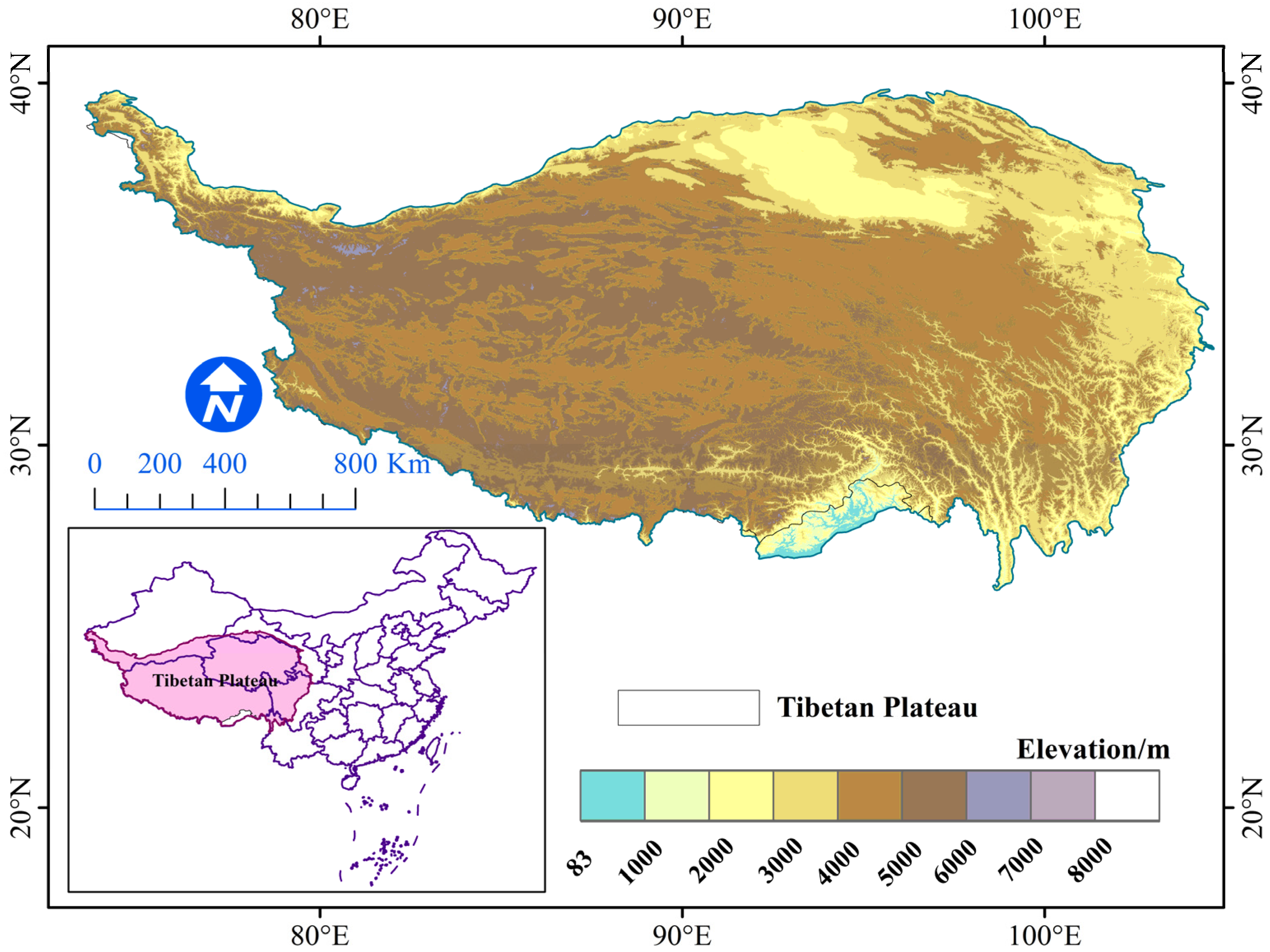
2.1. Study Area

The Third Pole is a high-elevation area in China centered on the Tibetan Plateau, with an average altitude exceeding 4000 m in Figure 1. The climate at the Third Pole is characterized by strong solar radiation, low air temperature, and large day–night temperature differences [36]. The temperature at the Third Pole is consistently low, with an annual average temperature below 0 °C throughout the region. Consequently, the Third Pole experiences a prolonged frost period and a relatively short growing season [37]. The distribution of vegetation is determined by the precipitation gradient, resulting in alpine meadows in the east, alpine steppe in the central area, and desert grassland in the west [38,39]. In this study, the responses of alpine vegetation to frost days were investigated in the central and eastern study areas.

2.2. Meteorological Forcing Datasets

The spatially gridded meteorological dataset was obtained from the China Meteorological Forcing Dataset (CMFD) provided by the National Tibetan Plateau Data Center (https://data.tpdc.ac.cn/, accessed on 19 April 2022). This dataset was created by integrating remote sensing products, reanalysis datasets, and in situ station data, and it is one of the most widely used climate datasets in China. This dataset has a temporal resolution of three hours and a spatial resolution of 0.1 degrees. In addition, the dataset includes seven near-surface meteorological elements such as 2 m air temperature (Ta) with a unit of K, surface pressure (P) with a unit of Pa, specific humidity (q) with a unit of kg kg⁻¹, 10 m wind speed (Us) with a unit of m s⁻¹, downward shortwave radiation (Rs) with a unit of W m⁻², downward longwave radiation (Rl) with a unit of W m⁻², and the precipitation rate with a unit of mm hr⁻¹. In this study, a long-term daily minimum temperature dataset in the Third Pole was obtained from the 3-hourly near-surface temperature elements. The frost days were based on a per-pixel basis in this dataset and were identified through the frost day estimation methods from a previous study at both the growing season and seasonal scales. Additionally, monthly datasets of air temperature, precipitation, and downward shortwave radiation were utilized to analyze how the frost days and climate factors respond differently to vegetation growth on the Third Pole.

2.3. Satellite Remote Sensing Datasets

The Moderate Resolution Imaging Spectroradiometer (MODIS) Land Cover Dynamics (MCD12Q2) dataset was available at yearly intervals and a 500 m spatial resolution. This product was derived from a time series of the 2-band enhanced vegetation index (EVI2), which was calculated from the MODIS Nadir Bidirectional Reflectance Distribution Function (BRDF)-Adjusted Reflectance (NBAR). Collection 6 of the MCD12Q2 dataset, which covered the period from 2001 to 2018 in the Third Pole, was obtained from Google Earth Engine (https://earthengine.google.com/, accessed on 27 April 2022). The Greenup and Greendown of the MCD12Q2 SDS layers were selected to extract the start of the season (SOS) and end of the season (EOS).

The MODIS NDVI dataset (MOD13A3) was available at monthly intervals and a 1 kilometer (km) spatial resolution. The products were computed from atmospheric corrected surface reflectance, which accounted for the removal of molecular scattering, ozone absorption, and aerosols. Collection 6 of the MOD13A3 from 2001 to 2018 in the Third Pole was accessible through the USGS website (https://search.earthdata.nasa.gov/, accessed on 19 June 2022). Some images were preprocessed to remove null values (−3000) and display only the values within the range of −2000 to 10000, as stated in the user guide. The original images were resampled to align with the spatial resolution of the meteorological forcing datasets (0.1°). Monthly images were created by calculating the mean value of each pixel. To eliminate the effects of cloud cover and snow contamination on the NDVI in high-elevation areas, the pixels with NDVI < 0 were replaced by 0.

The global OCO-2-based SIF product (GOSIF) was available at an 8-day resolution (as well as at monthly and annual resolutions) and 0.05-degree spatial resolution during the period of 2000–2021. This GOSIF product was derived from discrete OCO-2 SIF soundings, remote sensing data from the MODIS, and meteorological reanalysis using a data-driven method [31]. The product also had advanced spatial and temporal resolutions and much longer records compared with the coarse-resolution gridded SIF data that were directly aggregated from OCO-2 SIF soundings [31]. The spatial patterns and seasonal cycles of the GOSIF showed consistency with the coarse SIF data, and these strongly correlated with independent GPP data from 91 tower sites [31]. A detailed description of the GOSIF data (production, verification, and application) can be found in the GOSIF user guide. The monthly images were preprocessed to remove null values (32,767 and 32,766) and were resampled to spatially match the spatial resolution of the meteorological forcing datasets (0.1° spatial resolution). Pixels with GOSIF < 0 were replaced with 0. The monthly GOSIF data were used in this study to examine the spatial and temporal changes and trends of alpine vegetation in the Third Pole from 2001 to 2018. The relationship between the GOSIF data and environmental factors (frost days, air temperature, precipitation, and radiation) was discussed at both the growing season and seasonal scales.

The digital elevation model (DEM) data for the Third Pole was obtained from the Shuttle Radar Topography Mission (https://earthexplorer.usgs.gov/, accessed on 19 April 2023), with a spatial resolution of 30 m. The boundary of the Third Pole was acquired from the Global Change Research Data Publishing & Repository (https://www.geodoi.ac.cn/ , accessed on 19 April 2023) [40].

2.4. Estimating Methods of Frost Days

Frost days were defined as days when the T_min was below the freezing point of water (0 °C) [39]. Following this definition, the number of frost days in each season and in the entire growing season in the Third Pole from 2001 to 2018 were calculated. The seasonal frost days for spring (SPR_FDs), summer (SUM_FDs), and autumn (FAL_FDs) were calculated as the number of frost days from the SOS to the summer solstice, from 1 June to 31 August, and from the summer solstice to the EOS, respectively. The growing season frost days (GS_FDs, from the SOS to EOS) were calculated as the number of frost days from the SOS to EOS for each pixel. The formulas were expressed as follows:

$$SPR\_FDs={\displaystyle {\sum }_{SOS}^{summer\mathrm{solstice}}frost\begin{array}{cc}days& \end{array}}$$

(1)

$$SUM\_FDs={\displaystyle {\sum }_{1June}^{31August}frost\begin{array}{cc}days& \end{array}}$$

(2)

$$FAL\_FDs={\displaystyle {\sum }_{summer\mathrm{solstice}}^{EOS}frost\begin{array}{cc}days& \end{array}}$$

(3)

$$GS\_FDs={\displaystyle {\sum }_{SOS}^{EOS}frost\begin{array}{cc}days& \end{array}}$$

(4)

where the frost day algorithm differs in different time periods; the summer solstice is on 22 June in the Northern Hemisphere.

2.5. Processing of NDVI and GOSIF Data

The seasonal ranges mentioned in the frost day estimation methods were used to calculate the average GOSIF and NDVI values in the growing season and in each season. The dynamic changes in alpine vegetation were analyzed. The seasonal average GOSIF and NDVI values for spring (SPR_GOSIF/NDVI), summer (SUM_GOSIF/NDVI), and autumn (FAL_GOSIF/NDVI) were calculated as the average monthly GOSIF and NDVI values from the SOS to the summer solstice, from 1 June to 31 August, and from the summer solstice to the EOS, respectively. The growing season average GOSIF and NDVI (GS_GOSIF/NDVI) values were calculated as the average GOSIF and NDVI values from the SOS to EOS. In particular, the phenology values (day of the year) for each pixel were transformed into monthly values to generate seasonal and growing season GOSIF and NDVI values based on the monthly GOSIF and NDVI values for each pixel. The formulas were calculated as follows:

$$\mathrm{SPR}\_\mathrm{GOSIF}={\displaystyle {\sum }_{SOS\to SO{S}_{month}}^{\mathrm{summersolstice}\to summersolstic{e}_{month}}\overline{(GOSI{F}_{month})}}$$

(5)

$$SUM\_GOSIF={\displaystyle {\sum }_{June}^{August}\overline{(GOSI{F}_{month})}}$$

(6)

$$FAL\_GOSIF={\displaystyle {\sum }_{summersolstice\to summersolstic{e}_{month}}^{EOS\to EO{S}_{month}}\overline{(GOSI{F}_{month})}}$$

(7)

$$G\mathrm{S}\_\mathrm{GOSIF}={\displaystyle {\sum }_{SOS\to SO{S}_{month}}^{EOS\to EO{S}_{month}}(\overline{GOSI{F}_{month}})}$$

(8)

where the NDVI was calculated in the same way.

2.6. Statistical Analysis

The linear trends in frost days were calculated using the Mann–Kendall method. The Mann–Kendall method is a nonparametric test for monotonic trends [41,42]. This method does not assume a specific distribution for the data and is not sensitive to outliers. The Theil–Sen method was used to calculate the slope of the linear trend [43]. The slope of the trend was determined by the rate of change in the number of frost days over time. Furthermore, the Pearson correlation method was employed to calculate the correlation coefficients between vegetation parameters (e.g., SIF or NDVI) and various environmental factors, such as frost days, temperature, precipitation, and radiation. Correspondingly, the absolute values of the correlation coefficients were compared, reclassified, and used to identify the controlling factors for each pixel in the Third Pole from 2001 to 2018. To investigate the influences of the statistical methods on the interpretation of the effects of frost days (FD), temperature (Temp), precipitation (Pre), and shortwave radiation (Srad) on alpine vegetation (i.e., NDVI and SIF), the ridge regression (RR) method to solve the regression models [44] was used. Analyses based on satellite observations were used to determine the effects of environmental factors on alpine vegetation.

3. Results

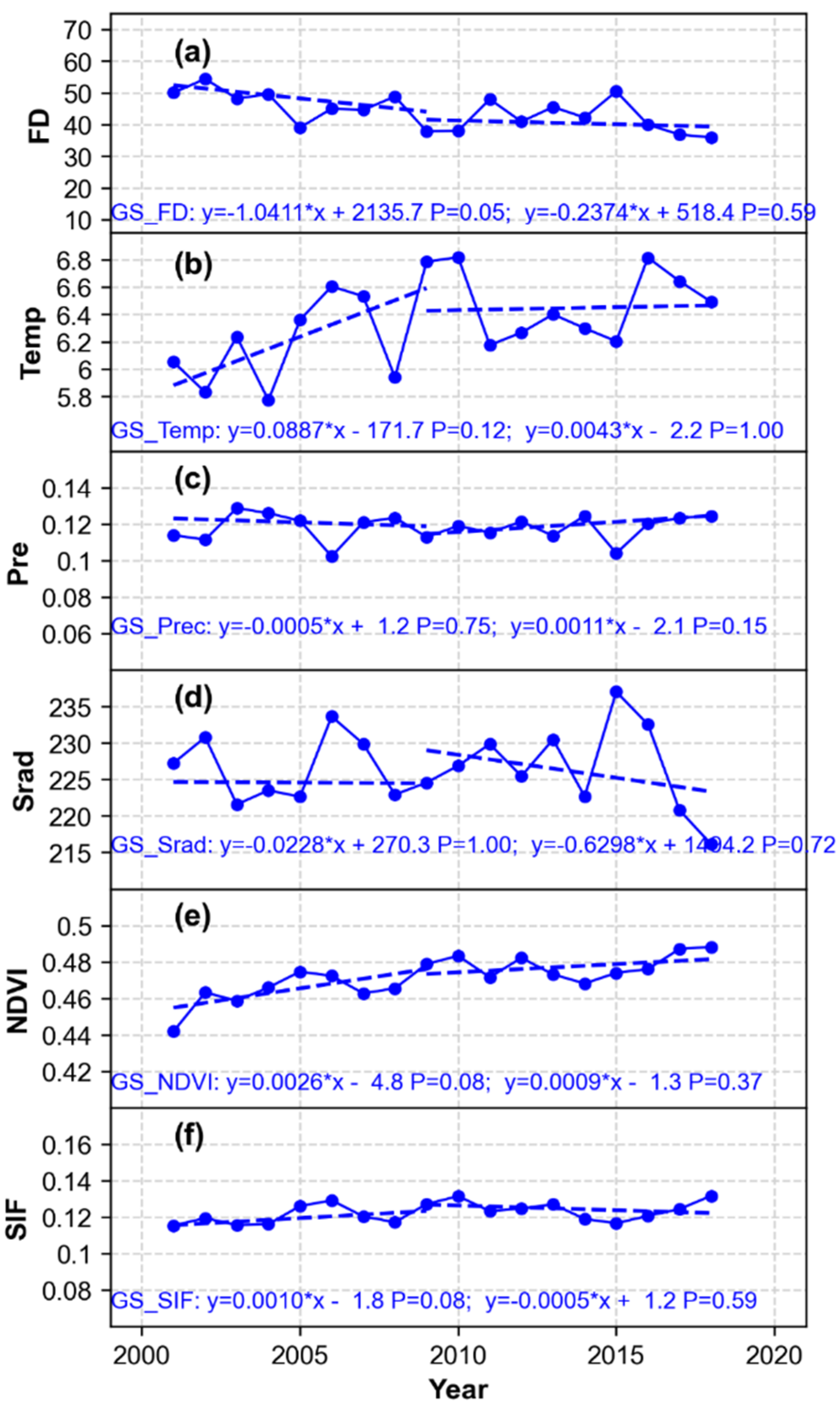
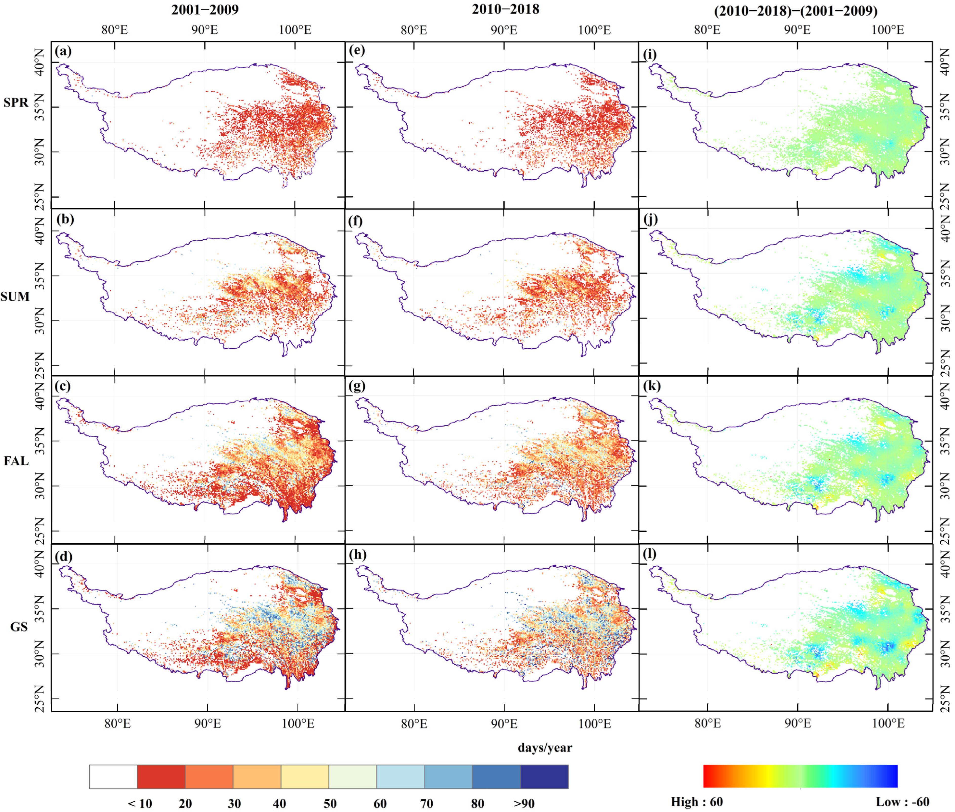
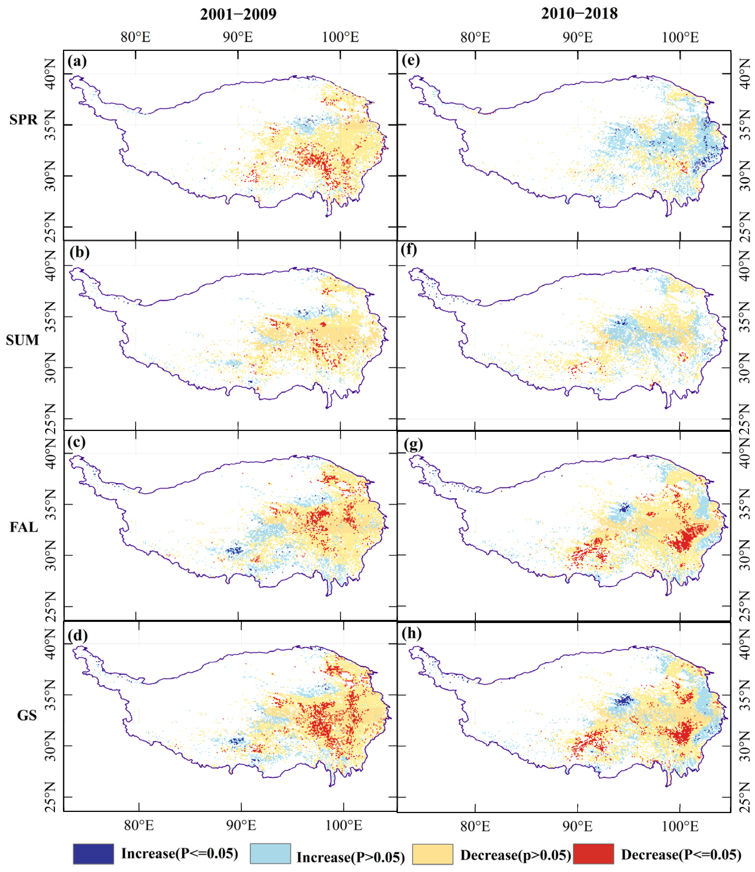
3.1. Spatiotemporal Patterns and Trends of Seasonal Frost Days from 2001 to 2018 in the Third Pole

The seasonal trends of environmental factors (frost days, temperature, precipitation, and radiation) and vegetation changes (GOSIF and NDVI) for each grid cell in the Third Pole during the period 2001–2018 were calculated by using the Mann–Kendall method. To highlight the effects of interannual variation for comparison, the seasonal trends of environmental factors and vegetation changes were examined in the Third Pole before and after 2010. Frost days (FDs) decreased significantly before 2010 (slope = −1.0411 days decade−1, p = 0.05) but had no significant trend after 2010 (slope =  −0.2374 days decade−1, p  =  0.59), as shown in Figure 2a. Temp had no significant increasing trend before and after 2010, as shown in Figure 2b. Pre had no significant decreasing trend before 2010 and an increasing trend after 2010, as shown in Figure 2c. Srad had no significant decreasing trend before and after 2010, as shown in Figure 2d. Additionally, the vegetation index such as NDVI and GOSIF increased significantly (p < 0.1) before 2010, while no significant trends occurred after 2010, as shown in Figure 2e,f.

The FDs at the growing season and seasonal scales for each grid cell on the Tibetan Plateau during the period of 2001–2018 were estimated from the CMFD datasets in Figure 3. To highlight the effects of the decadal differences in Tmin on FDs, we first separately analyzed the spatial patterns of FDs in the periods of 2001–2009 and 2010–2018 and then compared the differences between the two periods. From 2001 to 2009, the average SPR_FDs, SUM_FDs, FAL_FDs, and GS_FDs in the Third Pole were about 12.71 days, 18.41 days, 33.89 days, 43.89 days, respectively. From 2010 to 2018, the average SPR_FDs, SUM_FDs, FAL_FDs, and GS_FDs in the Third Pole were about 11.02 days, 15.17 days, 31.03 days, and 41.97 days, respectively. By comparison, there are some differences between before and after 2010 in the FDs at the growing season and seasonal scales. At length, the magnitudes of the FAL_FDs and GS_FDs before 2010 and after 2010 were close. Due to the relatively short summer on the Tibetan plateau, the number of frost days in summer and spring is more or less the same. Geographically, the spatial patterns of the FDs during the periods of 2001–2009 and 2010–2018 were consistent with the larger area of the Third Pole. The central Qinghai Plateau was more exposed to an increasing occurrence of FDs. The spatial variation patterns of FDs in different seasons (except in spring) were similar to those of the growing season FDs. Overall, the FDs in the Third Pole revealed divergent geographical differences among growing season and seasonal cycles between 2001–2009 and 2010–2018.

Examining different research periods led to different results that could not be directly verified and compared to each other; thus, comparative analysis could not be performed among multiple periods. Figure 4 shows the temporal trends in FDs during the growing season and seasonal scales in the Third Pole during periods of different lengths starting between 2000 and 2018. Overall, the FDs at the growing season and seasonal scales had no significant decreasing trends in the Third Pole from 2001 to 2018. Specially, the trend values of SPR_FDs, SUM_FDs, FAL_FDs, and GS_FDs at different research periods ranged from −0.4 to 0.4, and most of these values were less than 0, which means that the FDs at the growing season and seasonal scales in different study periods showed insignificant decreasing trends in Figure 4a–d. The FD trends during the periods of 2005–2015, 2006–2015, and 2007–2015 exhibited statistically insignificant increasing patterns. Conversely, the FD trends for the two intervals commencing in 2001 and 2002 demonstrated a rapid decline, with a considerable number of periods passing the significance test. The FAL_FDs trend was close to that of the GS_FDs and decreased by a similar magnitude. Overall, decreasing trends of FDs were found in the Third Pole from 2001 to 2018, which were generally consistent with the results of previous studies and helped clarify FD trends during different research periods.

3.2. Effects of Heatwaves on Vegetation

To compare the differences in the FD trends, the FD trends in the Third Pole in both the 2001–2009 and 2010–2018 periods were examined in Figure 5. For the period of 2001–2009, the percentage of pixels with decreasing trends in SPR_FDs, SUM_FDs, FAL_FDs, and GS_FDs accounted for 12.70%, 11.60%, 14.33%, and 16.32%, respectively. The percentages of pixels with increasing trends in SPR_FDs, SUM_FDs, FAL_FDs, and GS_FDs accounted for 1.39%, 1.82%, 4.32%, and 3.23%, respectively. For the period of 2010–2018, the percentage of pixels with decreasing trends in SPR_FDs, SUM_FDs, FAL_FDs, and GS_FDs accounted for 7.71%, 5.01%, 4.02%, and 5.51%, respectively. The percentages of pixels with increasing trends in SPR_FDs, SUM_FDs, FAL_FDs, and GS_FDs accounted for 4.73%, 7.48%, 14.92%, and 13.98%, respectively. Both the FAL_FDs and GS_FDs from 2001 to 2018 had similar spatial distributions of pixels with increasing or decreasing trends, while the SPR_FDs (2010 to 2018) had a larger area of pixels with increasing trends than that of pixels with decreasing trends. The SUM_FDs trends were different from those of SPR_FDs and FAL_FDs. Moreover, the pixels with no significant decreases (p > 0.05) in FD trends accounted for the largest and most widespread area during the entire period in the Third Pole. Geographically, the SPR_FDs and SUM_FDs showed significant increasing trends (2001–2009) and no significant decreasing trends (2010–2018) at the junction of the Qinghai Plateau, Western Plateau, and Tibetan Plateau. The FAL_FDs displayed increasing trends in the western part of the Qinghai Plateau and the central Third Pole and decreasing trends on the eastern plateau (2010–2018). The spatial patterns of FAL_FDs and GS_FDs trends coincided greatly in the Third Pole. Overall, the FD trends exhibited greater heterogeneity between the two periods and different seasonal cycles.

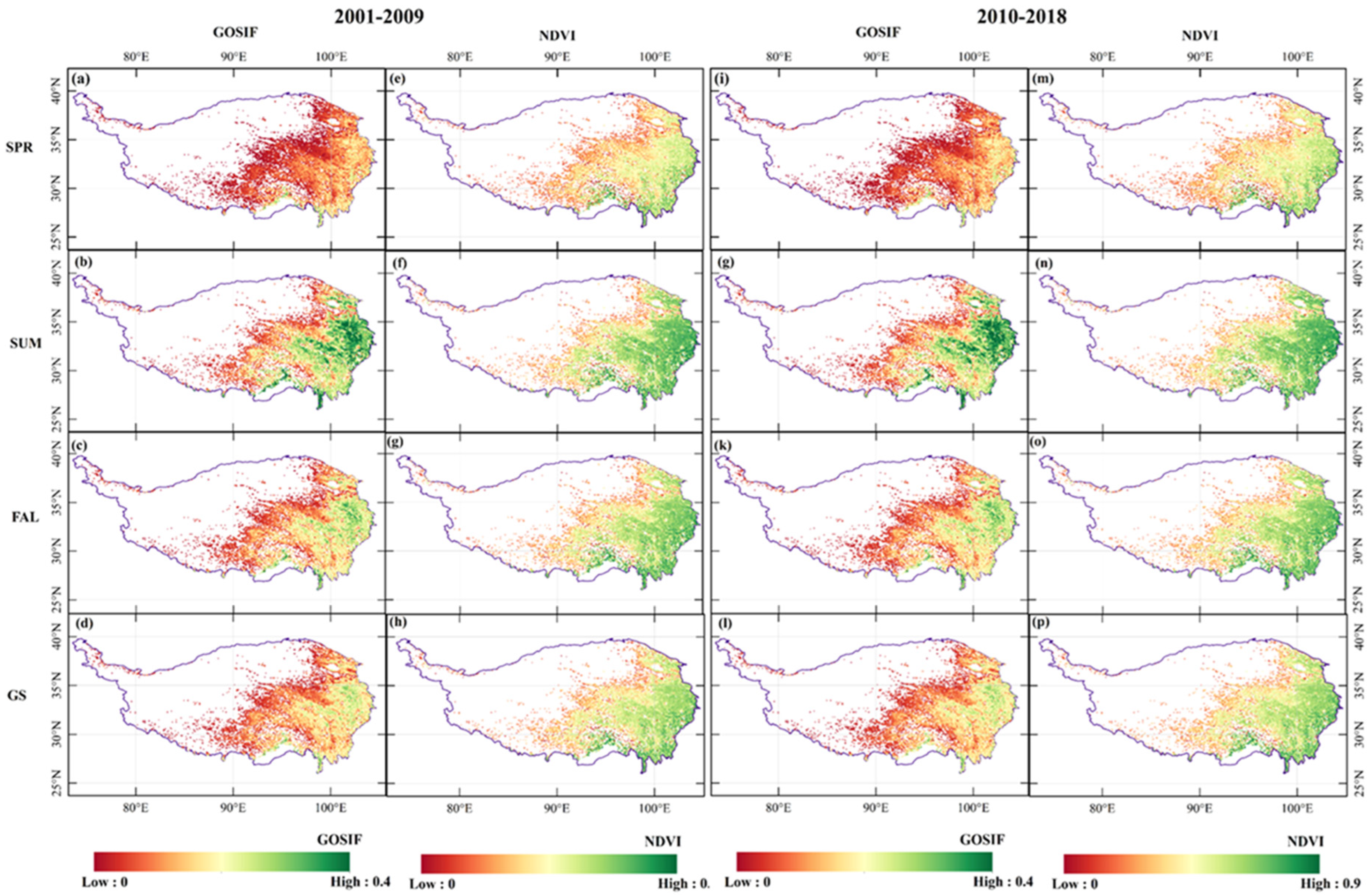
3.3. Spatiotemporal Patterns and Trends of Seasonal GOSIF and NDVI Data from 2001 to 2018 on the Third Pole

The GOSIF and NDVI patterns were also calculated in the same way as the FD was calculated in Figure 6. The temporal trends in the GOSIF and NDVI values at the growing season and seasonal scales in the Third Pole during periods of different lengths starting between 2000 and 2018 are shown in Figure 7. In particular, the GOSIF trend values ranged from −0.002 to 0.002, and most of them were less than 0, which meant that the GOSIF at the growing season and seasonal scales in different study periods showed no statistically increasing or decreasing trend (Figure 7a–d). The NDVI trend values ranged from −0.004 to 0.004, and most of them were greater than 0, which meant that the NDVI at the growing season and seasonal scales in different study periods showed an insignificant increasing trend (Figure 7e–h). Generally, the GOSIF and NDVI trends showed obvious differences with the change in season due to the periodicity of the vegetation. The GOSIF trends for the later columns (starting from 2003 to 2010) showed a decline, and a relatively large number of periods passed the significance test. The NDVI trends in each of the different study periods showed an increasing trend. Generally, the GOSIF and NDVI trends at the growing season and seasonal scales showed an increasing or decreasing trend from 2001 to 2018, which was most likely due to the different internal mechanisms between the NDVI and GOSIF.

To compare the spatial distribution of the GOSIF and NDVI trends in different seasonal cycles, the GOSIF and NDVI trends in the Third Pole during 2001–2018 are shown in Figure 8. Overall, the GOSIF and NDVI between the periods of 2001–2009 and 2010–2018 showed the largest area with increasing trends and the smallest area with decreasing trends. The seasonal GOSIF and NDVI trends exhibited similar spatial patterns, but the spatial differences were still apparent. The spatial patterns of the GOSIF values were obviously clearer than those of the NDVI. The explanation for this is that the GOSIF product can monitor seasonal physiology and capture seasonal plant photosynthetic responses in Figure 7. Therefore, understanding the seasonal dynamics of alpine vegetation is a key step in comprehending the seasonal vegetation response to environmental factors. Moreover, our results suggest that both the GOSIF and NDVI can help clarify the differences among and the information provided by the seasonal variations in the vegetation structure, greenness, and physiology at regional scales in the Third Pole.

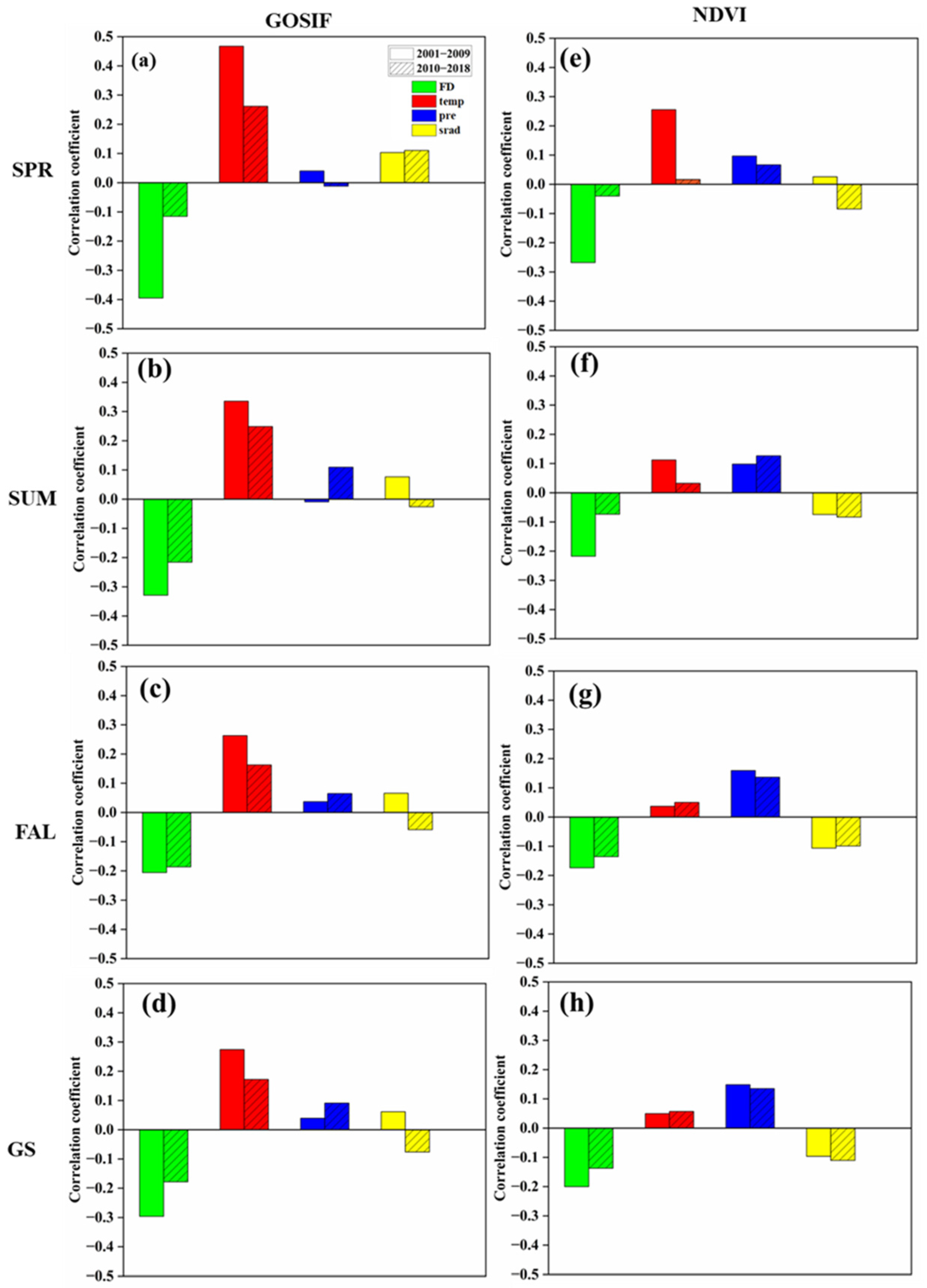
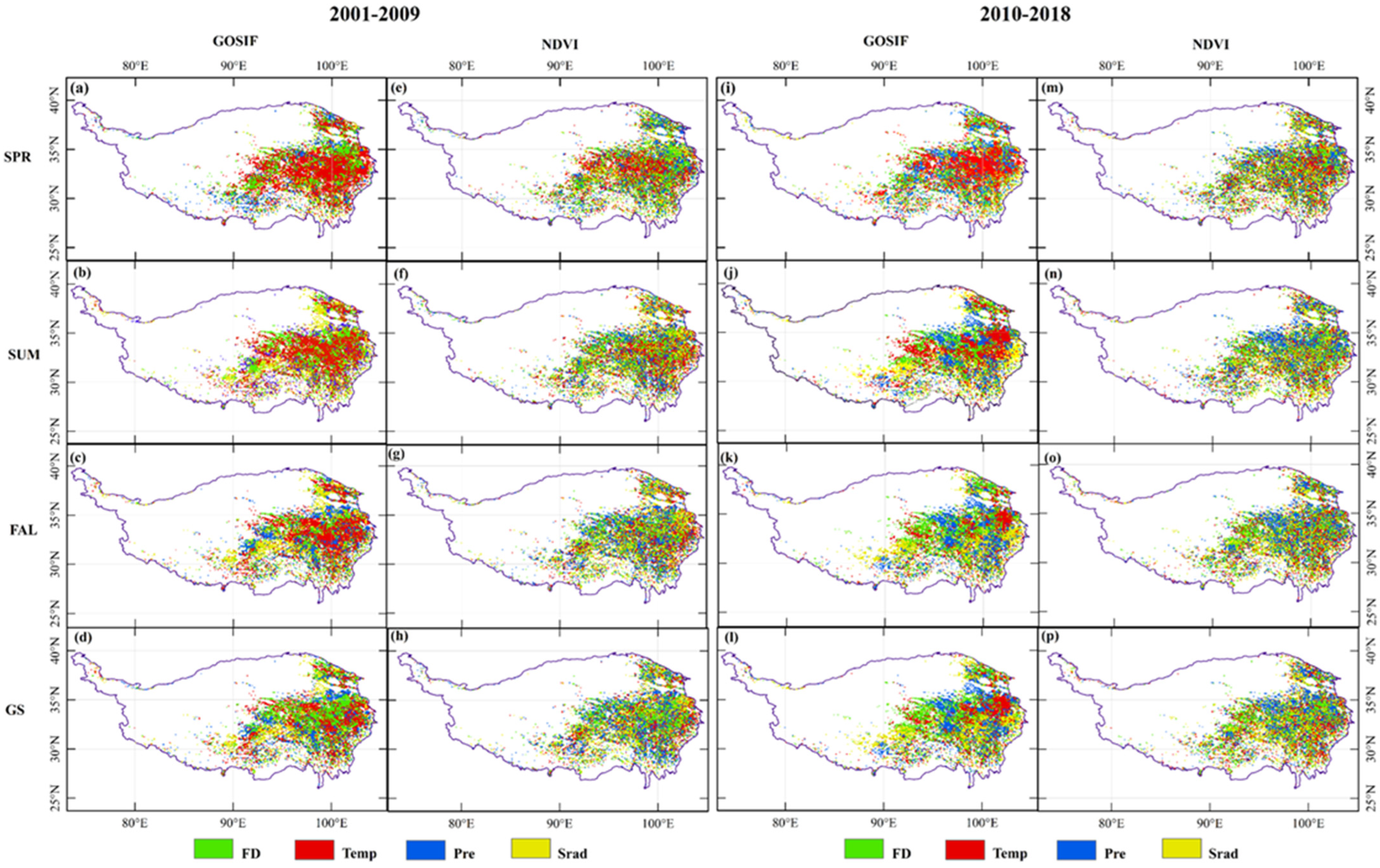
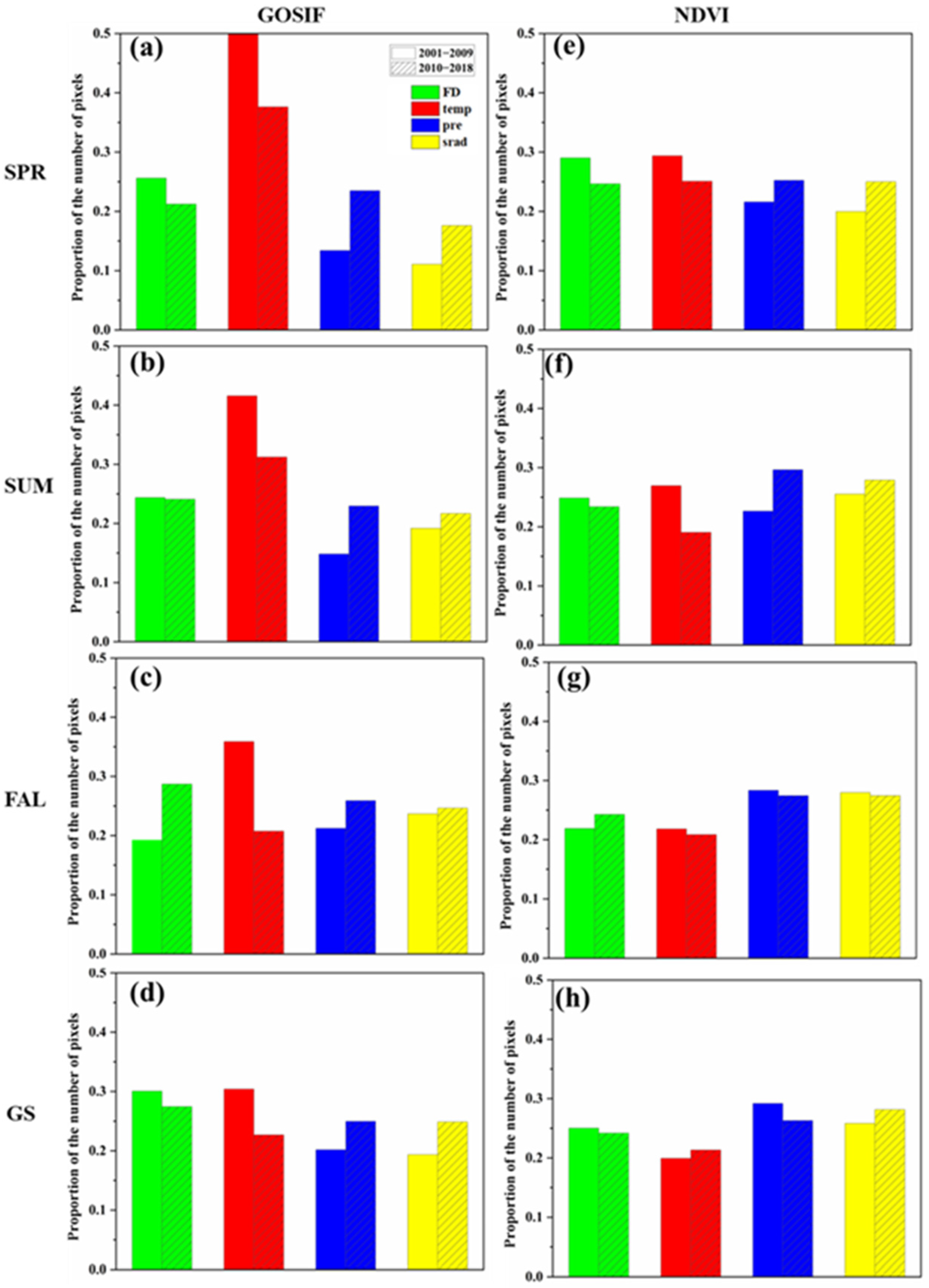
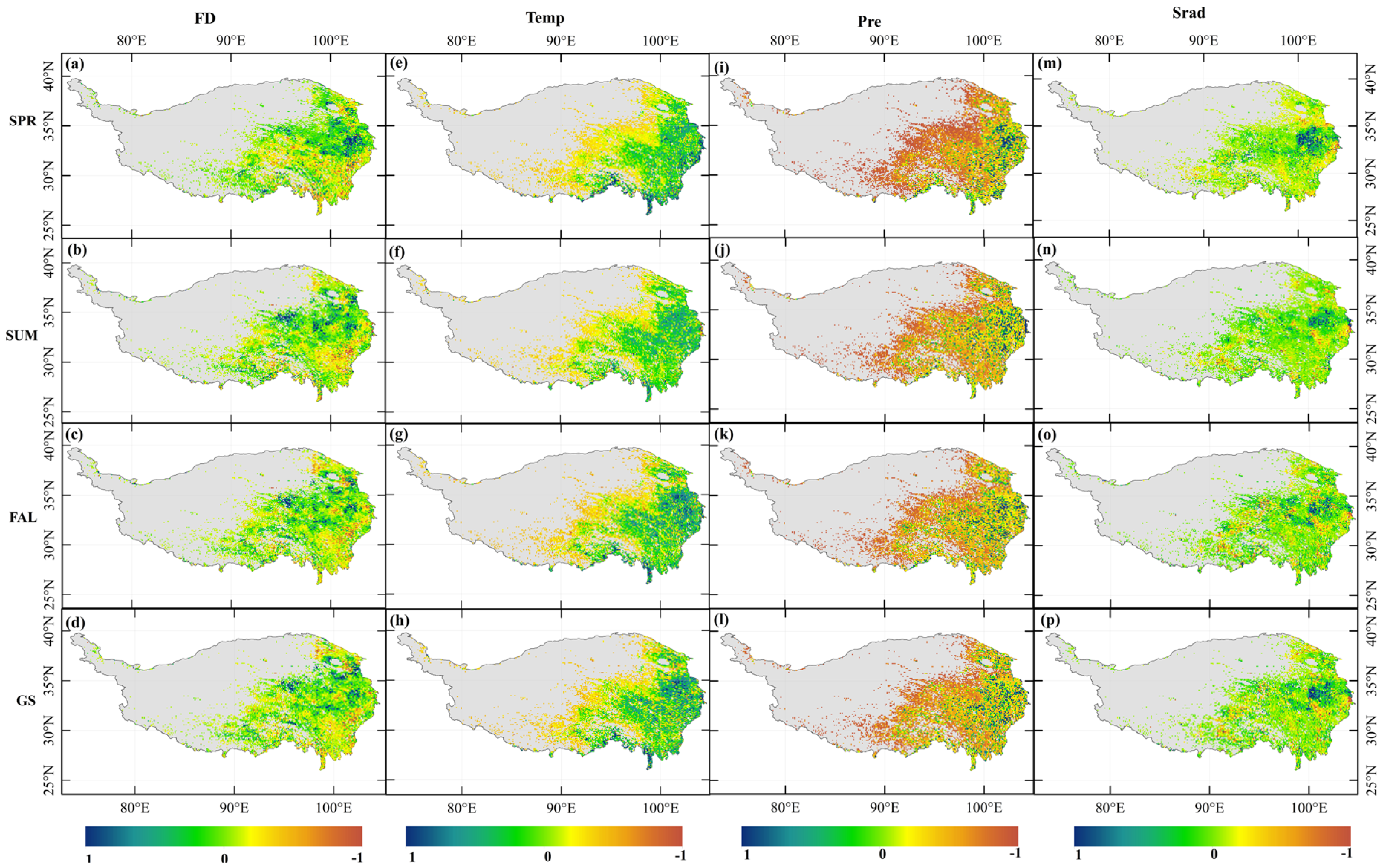
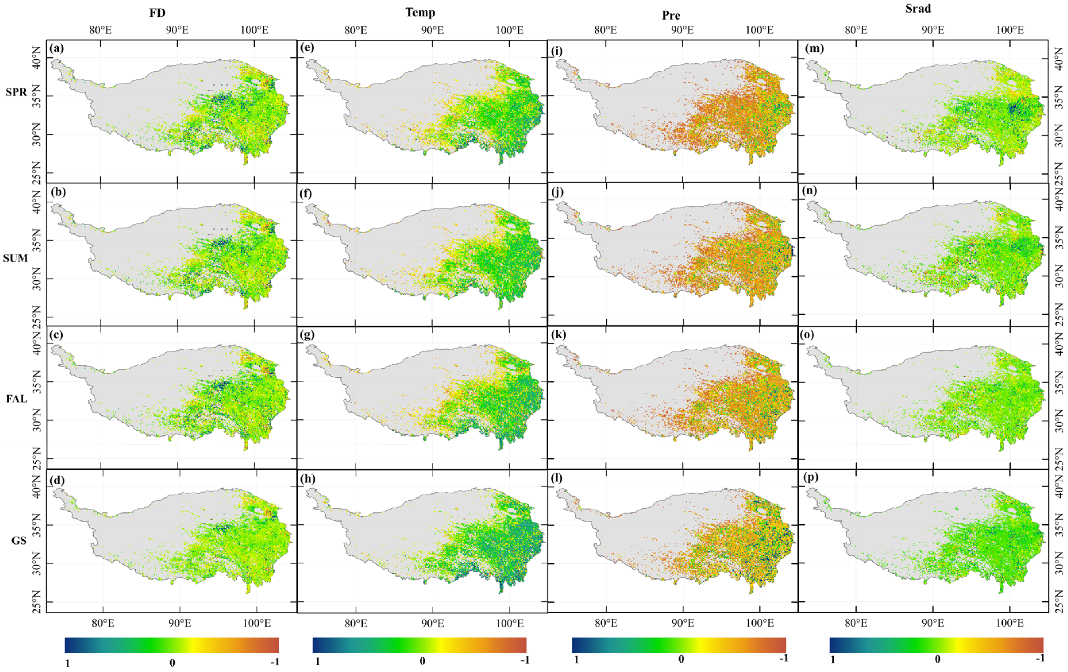
3.4. Effects of Environmental Factors on Seasonal GOSIF and NDVI Values

To examine the environmental controls on alpine vegetation, the controlling effects of environmental factors (FDs, Temp, Pre, and Srad) on GOSIF and NDVI values in both 2001–2009 and 2010–2018 were analyzed and shown in Figure 9. In each period, the GOSIF and NDVI values showed different relationships with the environmental factors at different seasonal scales. Among these environmental factors, the number of frost days had negative relationships with GOSIF and NDVI values. The air temperature had positive relationships with GOSIF and NDVI values. Other environmental factors, such as precipitation and radiation, had opposite effects in the two periods. By comparison, the correlation coefficient between the GOSIF-FDs and NDVI-FDs during 2001–2009 was greater than that during 2010–2018. This indicated that the relationship between GOSIF-FDs and NDVI-FDs weakened from 2001 to 2018. Similarly, the difference between the coefficients of the two periods was used to evaluate the effects of environmental factors on the variation in the interannual correlation coefficients. During the two periods, declines in sensitivity were also seen in both GOSIF-FDs and NDVI-FDs. Similarly, during the two periods, declines in sensitivity were also seen in both GOSIF-Temp and NDVI-Temp. The difference between GOSIF-Pre and GOSIF-Srad was greater than that between NDVI-Srad and NDVI-Pre, indicating that the sensitivity of GOSIF and NDVI was divergent owing to the functional and structural characteristics of the vegetation. In terms of seasonal scales, temperature was one of the major controlling factors of the vegetation, followed by frost, with precipitation and radiation having the least influence. Considering that the seasonal change in alpine vegetation in the Third Pole is the result of the comprehensive action of many meteorological factors, no single factor explained the change to a high degree. This study indicated greater variability in the correlation coefficients between GOSIF and environmental factors compared to NDVI during the growing season. Notably, the differences in correlation coefficients between environmental factors and vegetation parameters were significant. Furthermore, the GOSIF product was superior to the NDVI in detecting frost impacts.

To identify which environmental factors control alpine vegetation, we further compared the absolute values of these correlation coefficients for each pixel, reclassified four groups, and obtained the spatial distribution of the controlling factors in the growing season in the Third Pole from 2001 to 2018, as shown in Figure 10. Overall, large spatial heterogeneity existed in the temporal evolution of controlling factors. The discrepancies in controlling factors among the different vegetation datasets mainly resulted from the differences in the data. Most of the central plateau was mainly controlled by temperature, which was most obvious in spring. The northern Qinghai Plateau was controlled by frost days, which was most significant in the growing season, according to the trends and magnitudes of the frost days from 2001 to 2018. The southwest and northeast regions of the plateau were affected by radiation. The contribution of precipitation was more obvious in the period of 2010–2018 according to its distribution, but there was no regularity in the period of 2001–2009, indicating a positive influence on the sensitivity of vegetation growth to precipitation. Furthermore, the GOSIF values had a higher correlation with environmental factors, and the contribution of each environmental factor in each season over the whole region was regularly distributed.

The proportion of pixels showed the relative contribution of different environmental factors to the interannual variation in the GOSIF and NDVI values from 2001 to 2018 in the Third Pole (Figure 11). Overall, the proportion of pixels for the GOSIF and NDVI showed consistent trends. Due to climate change, the controlling factors of interannual variation in vegetation photosynthesis in the Third Pole have gradually changed from temperature to precipitation. The controlling effects of temperature and frost days both decreased, while the controlling effects of precipitation and radiation increased. Temperature was found to have the greatest effect on alpine vegetation in spring, frost was found to have the least effect on alpine vegetation in summer, and radiation and precipitation had the least effect on alpine vegetation in autumn. In addition, the spatial variability of the sensitivities of the GOSIF and NDVI to FD, Temp, Pre, and Srad based on the results derived from the four-variable RR method were investigated (Figure 12 and Figure 13). Interestingly, our results demonstrate that the seasonal patterns of the effects of each environmental variable on GOSIF show a close agreement with the seasonal patterns of the effects of each environmental variable on NDVI. More importantly, temperature had a positive effect on vegetation growth in the eastern part of the Third Pole.

4. Discussion

For the first time, a comprehensive study was conducted on a regional scale to investigate the effects of frost on alpine vegetation at different timescales (growing season and seasonal scales) by combining a daily meteorological forcing dataset with a remotely sensed phenology dataset. The results of our study indicated a reduction in the number of frost days during the growing seasons in the Third Pole, indicating reduced exposure of alpine vegetation to freezing events due to climate warming. A recent study examined the spatial–temporal changes in extreme temperature events over Tibet for the period of 1961–2010 and also found a significant reduction in the number of frost days (days with daily minimum temperature < 0 °C per year) [45]. The findings of some studies were inconsistent with our results; they calculated the number of frost days over the whole year, neglecting the influence of different seasons. Given the relatively short growing season on the Tibetan Plateau, an annual calculation of frost days would overlook seasonal variations. Some researchers divided the growing season into spring and autumn and examined the period spanning 1982–2012 in the Northern Hemisphere. Their findings also indicated a substantial reduction in the number of frost days on the Tibetan Plateau [46], aligning with our own results. Other studies mentioned that spring frost events emerged as the main driving factors influencing the spring phenology of cold-climate vegetation [47]. One study reported contrasting trends in late spring frost occurrences between 1959 and 2017: a decrease in North America and an increase in Europe and Asia [8]. Another study also analyzed spring frost on the southeastern Tibetan Plateau using in situ observational phenological data. Their study revealed that spring frost exerted control over elevational gradients on the spring phenology [35]. Overall, there are very few studies investigating frost events at various timescales on the Third Pole. Variations in seasonal parameters within the frost calculation algorithm can yield markedly distinct estimates of the number of frost days. Therefore, we still lack a comprehensive understanding of broad-scale spatial and temporal patterns in frost events.

Using satellite-based NDVI and SIF products [27,48], we provided a comprehensive assessment of the spatial–temporal variations and trends in vegetation greenness and photosynthesis in the Third Pole region from 2001 to 2018. Our findings revealed a clear east-to-west gradient of decreasing NDVI and SIF values, consistent with the climatic characteristics of the Tibetan Plateau (Figure 6). While both the NDVI and SIF values showed slight increases from 2001 to 2018 across the Third Pole, the seasonal SIF patterns slightly deviated from those of the NDVI (Figure 7), aligning with most previous findings [49,50]. However, in spring, the SIF exhibited a heterogeneous spatial distribution without a clear spatial pattern. It was previously unknown whether the SIF dataset repeated the spatial pattern found in the NDVI dataset despite the same extraction algorithms applied to these two datasets [51]. Both the NDVI and SIF values contributed to differences in the mean changes in the SIF and NDVI during each stage of the growing season. Consequently, the spatiotemporal variations and trends in the SIF and NDVI in each growing season are the basis for studying the response of alpine vegetation to frost events. It is still crucial to study frost events, assess actual plant damage, and characterize the response of alpine vegetation to frost events during each season of the growing season on the Third Pole.

Currently, evaluating the impact of frost on alpine ecosystems has become a hot topic. Plant responses to frost vary across plant-specific growth stages [13]. However, in the Third Pole, where the frost intensity is higher, the earlier dormancy release triggered by the higher air temperature in May increases the exposure of meristems to frost events. During the early stage of the growing season, vegetation growth is mainly controlled by temperature. Our results are consistent with those of previous research demonstrating the optimal adaptation of alpine vegetation to its high and cold environment. Nevertheless, the authors of these previous studies also pointed out that temperature played a key role in vegetation growth. They indicated that projected warmer temperatures could increase frost availability at the local scale, having a greater impact on alpine vegetation. It is critical to determine the physiological traits and thresholds affecting alpine vegetation during the frost period. The freezing resistance of plants has largely been regarded as reaching its seasonal minimum, without much variation, in summer months. Most studies merely show the potential correlation of vegetation dynamics with climatic variations (temperature and precipitation), thereby neglecting other crucial environmental variables [50]. Our results supported previous analyses, suggesting that temperature-related factors might be the main drivers of vegetation variability in the Third Pole, with less influence of precipitation, radiation, and frost (Figure 10). Due to climate change, the controlling effects of temperature and frost days were both decreasing, whereas those of precipitation and radiation were increasing. Overall, spring, summer, and autumn remain relatively crucial seasons in climate change studies within alpine ecosystems [15]. In contrast, no increase in the freezing resistance of the alpine vegetation was expected to occur at the end of summer, especially as it was undergoing senescence. Owing to climate change, the controlling effects of temperature and frost days were both decreasing, while those of precipitation and radiation were amplifying. Some people demonstrated a declining sensitivity to precipitation and an increasing sensitivity to temperature, which was not supported by our results [52]. Given the complexity of climate variation drivers, research on the sensitivity of alpine vegetation to climate change on the Third Pole needs to be integrated with a combination of factors. Overall, the long-term probability of frost might adjust the sensitivity of alpine vegetation to diverse environmental cues, thereby minimizing the exposure of its sensitive tissue to frost. Understanding how this change in sensitivity to environmental factors will affect the alpine vegetation growth response will be important for understanding regional drivers in future changes.

Changes in SIF exhibited greater magnitude compared to NDVI, implying vegetation photosynthesis is more sensitive to climate change than greenness, potentially due to variations in light use efficiency [53]. In this study, we found that SIF was more sensitive to frost events than the NDVI. As a direct proxy of photosynthesis, SIF demonstrated greater susceptibility to environmental stress compared to the traditional greenness-based NDVI [27]. SIF can serve as a good indicator in monitoring and assessing the impacts of extreme climatic events such as heatwaves, droughts, and frost on vegetation growth [54]. Some people found that satellite-based SIF observations exhibited a clear response to heat and water stress in vegetation from 2009 to 2010 across southern China, in contrast to the less pronounced response observed in the NDVI [19]. Others also found that SIF showed a significant reduction and an earlier response in winter wheat in northwestern India, whereas the NDVI and EVI could not capture the thermal stress effect [18]. Some scholars demonstrated that SIF could detect early-stage drought, while the NDVI could detect drought lasting over a long-time scale [20]. In line with most previous studies, heat and moisture stress tended to manifest earlier or in a more pronounced way in SIF than in the NDVI. Furthermore, they observed supplementary responses of different vegetation types [55]. Overall, most previous studies have shown that SIF data provide a new way to evaluate and estimate the impacts of environmental stress on vegetation growth. Integrating structural information from the NDVI and physiological information from GOSIF measurements will enhance our understanding of the alpine vegetation response to frost dynamics on the Third Pole.

There are certain limitations and uncertainties in this study. First, meteorological forcing data have a relatively sparse resolution, resulting in the occasional misidentification of frost days. The definition of frost days in most studies uses 0 °C as the freezing threshold, but this may result in uncertainties when comparing frost occurrences between the Third Pole and other regions [8]. Therefore, future studies still need ground-based observational data to validate the robustness of the calculation of frost days. Another limitation relates to satellite vegetation observations in the region. Additionally, NDVI products in the Third Pole, as measurements of vegetation activities, may also be affected by clouds, snow cover, or land degradation. Despite the superior spatial and temporal resolution of the GOSIF (0.05°) compared to earlier SIF products and its extensive data record spanning from 2000 to the present, compared to MODIS data, the GOSIF data are still subject to uncertainties arising from factors including meteorological reanalysis data, the quality of OCO-2 SIF, biases in the enhanced vegetation index, and imperfect modeling methods [31,56]. The different spatial representativeness among meteorological forcing data, MODIS NDVI data, MODIS phenology data, and OCO-2 GOSIF data can also lead to uncertainties in the study. Additionally, our study used only correlation analysis to study the relationship between the GOSIF or NDVI and environmental factors such as frost, temperature, precipitation, and radiation in different seasons. The diverse environmental influences on alpine vegetation were accessed in this study. Moreover, different vegetation types exhibited varied responses to frost, attributed to differences in photosynthetic capacity and metabolic capacities, as well as the duration of their required growing periods. Future studies could focus on frost events to analyze frost effects on different vegetation types and multi-source technology integration. By combining with leaf- and canopy-level auxiliary measurements, satellite SIF validation and mechanistic understanding of the relationship between SIF and photosynthesis are important in this study [57]. In other words, ground-observed SIF at local scales and satellite SIF at the regional scales would be valuable for examining the mechanisms in the future [58].

In the context of global climate change in alpine regions expected to be two to three times faster in the 21st century than in the 20th century [59], alpine ecosystems remain the areas most affected by future climate change and will continue to require significant attention in the future [60]. In order to mitigate the ecological, climatological, and social consequences of future climate change, we must understand and quantify the vulnerability of alpine ecosystems to climate variability. In fact, understanding vegetation dynamics of Alpine ecosystems can provide insight into future vegetation–climate feedback [61]. It would be beneficial to broader ecological and climatological implications, particularly in relation to the management of alpine ecosystems under climate change [62].

5. Conclusions

Based on the metrological forcing dataset and remote sensing datasets, this study quantitatively evaluated the frost days during the growing season and seasonal scales in the Third Pole in relation to long-term climate change and explored the relationship between vegetation changes and environmental factors during recent decades. We examined the spatial distribution patterns and temporal trends of frost days on the Third Pole from 2001 to 2018. Additionally, we estimated the spatial–temporal variations and trends of the NDVI and GOSIF during the growing season and seasonal scales on the Third Pole from 2001 to 2018. We further compared the absolute values of the correlation coefficients for each pixel, reclassified them into four groups, and subsequently obtained the spatial distribution of the controlling factors at the growing season and seasonal scales on the Third Pole from 2001 to 2018. Notably, some of the key conclusions were as follows. With rapid warming, frost days showed no significant decreasing trends from 2001 to 2018 on the Third Pole. The GOSIF data revealed a higher sensitivity of alpine vegetation to frost compared to the NDVI data. This study highlighted the importance of understanding frost events and revealed the diverse responses of NDVI and GOSIF values to frost events on the Third Pole.

References

1. Dittmar, C.; Fricke, W.; Elling, W. Impact of late frost events on radial growth of common beech (Fagus sylvatica L.) in Southern Germany. Eur. J. For. Res. 2005, 125, 249–259. [Google Scholar] [CrossRef]
2. Lamichhane, J.R. Rising risks of late-spring frosts in a changing climate. Nat. Clim. Chang. 2021, 11, 554–555. [Google Scholar] [CrossRef]
3. Chamberlain, C.J.; Wolkovich, E.M. Late spring freezes coupled with warming winters alter temperate tree phenology and growth. New Phytol. 2021, 231, 987–995. [Google Scholar] [CrossRef] [PubMed]
4. Hufkens, K.; Friedl, M.A.; Keenan, T.F.; Sonnentag, O.; Bailey, A.; O’Keefe, J.; Richardson, A.D. Ecological impacts of a widespread frost event following early spring leaf-out. Glob. Chang. Biol. 2012, 18, 2365–2377. [Google Scholar] [CrossRef]
5. Marquis, B.; Bergeron, Y.; Simard, M.; Tremblay, F. Growing-season frost is a better predictor of tree growth than mean annual temperature in boreal mixedwood forest plantations. Glob. Chang. Biol. 2020, 26, 6537–6554. [Google Scholar] [CrossRef]
6. Gerdol, R.; Siffi, C.; Iacumin, P.; Gualmini, M.; Tomaselli, M. Advanced snowmelt affects vegetative growth and sexual reproduction of vaccinium myrtillus in a sub-alpine heath. J. Veg. Sci. 2013, 24, 569–579. [Google Scholar] [CrossRef]
7. Vitasse, Y.; Rebetez, M. Unprecedented risk of spring frost damage in Switzerland and Germany in 2017. Clim. Chang. 2018, 149, 233–246. [Google Scholar] [CrossRef]
8. Zohner, C.M.; Mo, L.; Renner, S.S.; Svenning, J.-C.; Vitasse, Y.; Benito, B.M.; Ordonez, A.; Baumgarten, F.; Bastin, J.-F.; Sebald, V.; et al. Late-spring frost risk between 1959 and 2017 decreased in North America but increased in Europe and Asia. Proc. Natl. Acad. Sci. USA 2020, 117, 12192–12200. [Google Scholar] [CrossRef]
9. Bojórquez, A.; Martínez-Yrízar, A.; Álvarez-Yépiz, J.C. A landscape assessment of frost damage in the northmost Neotropical dry forest. Agric. For. Meteorol. 2021, 308–309, 108562. [Google Scholar] [CrossRef]
10. Deng, G.; Zhang, H.; Yang, L.; Zhao, J.; Guo, X.; Ying, H.; Rihan, W.; Guo, D. Estimating Frost during Growing Season and Its Impact on the Velocity of Vegetation Greenup and Withering in Northeast China. Remote Sens. 2020, 12, 1355. [Google Scholar] [CrossRef]
11. Ma, Q.; Huang, J.-G.; Hänninen, H.; Berninger, F. Divergent trends in the risk of spring frost damage to trees in Europe with recent warming. Glob. Chang. Biol. 2019, 25, 351–360. [Google Scholar] [CrossRef]
12. Allevato, E.; Saulino, L.; Cesarano, G.; Chirico, G.B.; D’URso, G.; Bolognesi, S.F.; Rita, A.; Rossi, S.; Saracino, A.; Bonanomi, G. Canopy damage by spring frost in European beech along the Apennines: Effect of latitude, altitude and aspect. Remote Sens. Environ. 2019, 225, 431–440. [Google Scholar] [CrossRef]
13. Neuner, G. Frost resistance in alpine woody plants. Front. Plant Sci. 2014, 5, 654. [Google Scholar] [CrossRef] [PubMed]
14. Nidzgorska-Lencewicz, J.; Mąkosza, A.; Koźmiński, C.; Michalska, B. Potential Risk of Frost in the Growing Season in Poland. Agriculture 2024, 14, 501. [Google Scholar] [CrossRef]
15. Neuner, G.; Huber, B.; Plangger, A.; Pohlin, J.-M.; Walde, J. Low temperatures at higher elevations require plants to exhibit increased freezing resistance throughout the summer months. Environ. Exp. Bot. 2020, 169, 103882. [Google Scholar] [CrossRef]
16. Ladinig, U.; Hacker, J.; Neuner, G.; Wagner, J. How endangered is sexual reproduction of high-mountain plants by summer frosts? Frost resistance, frequency of frost events and risk assessment. Oecologia 2013, 171, 743–760. [Google Scholar] [CrossRef]
17. Gallinat, A.S.; Primack, R.B.; Wagner, D.L. Autumn, the neglected season in climate change research. Trends Ecol. Evol. 2015, 30, 169–176. [Google Scholar] [CrossRef]
18. Song, L.; Guanter, L.; Guan, K.; You, L.; Huete, A.; Ju, W.; Zhang, Y. Satellite sun-induced chlorophyll fluorescence detects early response of winter wheat to heat stress in the Indian Indo-Gangetic Plains. Glob. Chang. Biol. 2018, 24, 4023–4037. [Google Scholar] [CrossRef]
19. Wang, X.; Qiu, B.; Li, W.; Zhang, Q. Impacts of drought and heatwave on the terrestrial ecosystem in China as revealed by satellite solar-induced chlorophyll fluorescence. Sci. Total Environ. 2019, 693, 133627. [Google Scholar] [CrossRef]
20. Liu, L.; Yang, X.; Zhou, H.; Liu, S.; Zhou, L.; Li, X.; Yang, J.; Han, X.; Wu, J. Evaluating the utility of solar-induced chlorophyll fluorescence for drought monitoring by comparison with NDVI derived from wheat canopy. Sci. Total Environ. 2018, 625, 1208–1217. [Google Scholar] [CrossRef]
21. Zhou, Z.; Ding, Y.; Liu, S.; Wang, Y.; Fu, Q.; Shi, H. Estimating the Applicability of NDVI and SIF to Gross Primary Productivity and Grain-Yield Monitoring in China. Remote Sens. 2022, 14, 3237. [Google Scholar] [CrossRef]
22. Tucker, C.J. Red and Photographic Infrared linear Combinations for Monitoring Vegetation. Remote Sens. Environ. 1979, 8, 127–150. [Google Scholar] [CrossRef]
23. Mohammed, G.H.; Colombo, R.; Middleton, E.M.; Rascher, U.; van der Tol, C.; Nedbal, L.; Goulas, Y.; Pérez-Priego, O.; Damm, A.; Meroni, M.; et al. Remote sensing of solar-induced chlorophyll fluorescence (SIF) in vegetation: 50 years of progress. Remote Sens. Environ. 2019, 231, 111177. [Google Scholar] [CrossRef] [PubMed]
24. Li, X.; Li, Y.; Chen, A.; Gao, M.; Slette, I.J.; Piao, S. The impact of the 2009/2010 drought on vegetation growth and terrestrial carbon balance in Southwest China. Agric. For. Meteorol. 2019, 269–270, 239–248. [Google Scholar] [CrossRef]
25. Wu, L.; Zhang, Y.; Zhang, Z.; Zhang, X.; Wu, Y.; Chen, J.M. Deriving photosystem-level red chlorophyll fluorescence emission by combining leaf chlorophyll content and canopy far-red solar-induced fluorescence: Possibilities and challenges. Remote Sens. Environ. 2024, 304, 114043. [Google Scholar] [CrossRef]
26. Qiu, R.; Li, X.; Han, G.; Xiao, J.; Ma, X.; Gong, W. Monitoring drought impacts on crop productivity of the US Midwest with solar-induced fluorescence: GOSIF outperforms GOME-2 SIF and MODIS NDVI, EVI, and NIRv. Agric. For. Meteorol. 2022, 323, 109038. [Google Scholar] [CrossRef]
27. Meroni, M.; Rossini, M.; Guanter, L.; Alonso, L.; Rascher, U.; Colombo, R.; Moreno, J. Remote sensing of solar-induced chlorophyll fluorescence: Review of methods and applications. Remote Sens. Environ. 2009, 113, 2037–2051. [Google Scholar] [CrossRef]
28. Baker, N.R. Chlorophyll fluorescence: A probe of photosynthesis in vivo. Annu. Rev. Plant Biol. 2008, 59, 89–113. [Google Scholar] [CrossRef]
29. Porcar-Castell, A.; Tyystjärvi, E.; Atherton, J.; van der Tol, C.; Flexas, J.; Pfündel, E.E.; Moreno, J.; Frankenberg, C.; Berry, J.A. Linking chlorophyll a fluorescence to photosynthesis for remote sensing applications: Mechanisms and challenges. J. Exp. Bot. 2014, 65, 4065–4095. [Google Scholar] [CrossRef]
30. Zhang, Y.; Guanter, L.; Berry, J.A.; Joiner, J.; van der Tol, C.; Huete, A.; Gitelson, A.; Voigt, M.; Köhler, P. Estimation of vegetation photosynthetic capacity from space-based measurements of chlorophyll fluorescence for terrestrial biosphere models. Glob. Chang. Biol. 2014, 20, 3727–3742. [Google Scholar] [CrossRef]
31. Li, X.; Xiao, J. A Global, 0.05-Degree Product of Solar-Induced Chlorophyll Fluorescence Derived from OCO-2, MODIS, and Reanalysis Data. Remote Sens. 2019, 11, 517. [Google Scholar] [CrossRef]
32. Duan, J.; Chen, L.; Li, L.; Wu, P.; Christidis, N.; Ma, Z.; Lott, F.C.; Ciavarella, A.; Stott, P.A. Anthropogenic Influences on the Extreme Cold Surge of Early Spring 2019 over the Southeastern Tibetan Plateau. Bull. Am. Meteorol. Soc. 2021, 102, S111–S116. [Google Scholar] [CrossRef]
33. Yin, H.; Sun, Y.; Donat, M.G. Changes in temperature extremes on the Tibetan Plateau and their attribution. Environ. Res. Lett. 2019, 14, 124015. [Google Scholar] [CrossRef]
34. Li, X.; He, L. Analysis of the February 2019 Atmospheric Circulation and Weather. Meteorol. Mon. 2019, 45, 738–744. [Google Scholar] [CrossRef]
35. Wang, Y.; Case, B.; Rossi, S.; Dawadi, B.; Liang, E.; Ellison, A.M. Frost controls spring phenology of juvenile Smith fir along elevational gradients on the southeastern Tibetan Plateau. Int. J. Biometeorol. 2019, 63, 963–972. [Google Scholar] [CrossRef] [PubMed]
36. Yao, T.; Xue, Y.; Chen, D.; Chen, F.; Thompson, L.; Cui, P.; Koike, T.; Lau, W.K.-M.; Lettenmaier, D.; Mosbrugger, V.; et al. Recent Third Pole’s Rapid Warming Accompanies Cryospheric Melt and Water Cycle Intensification and Interactions between Monsoon and Environment: Multidisciplinary Approach with Observations, Modeling, and Analysis. Bull. Am. Meteorol. Soc. 2019, 100, 423–444. [Google Scholar] [CrossRef]
37. Yu, H.; Luedeling, E.; Xu, J. Winter and spring warming result in delayed spring phenology on the Tibetan Plateau. Proc. Natl. Acad. Sci. USA 2010, 107, 22151–22156. [Google Scholar] [CrossRef]
38. Liu, D.; Wang, T.; Yang, T.; Yan, Z.; Liu, Y.; Zhao, Y.; Piao, S. Deciphering impacts of climate extremes on Tibetan grasslands in the last fifteen years. Sci. Bull. 2019, 64, 446–454. [Google Scholar] [CrossRef]
39. Chen, A.; Huang, L.; Liu, Q.; Piao, S. Optimal temperature of vegetation productivity and its linkage with climate and elevation on the Tibetan Plateau. Glob. Chang. Biol. 2021, 27, 1942–1951. [Google Scholar] [CrossRef]
40. Zhang, Y.; Li, B.; Zheng, D. Datasets of the Boundary and Area of the Tibetan Plateau. Acta Geogr Sin 2014, 69, 65–68. [Google Scholar]
41. Yan, B.; Lu, Z.; Li, J.; Huo, J. Analysis of Runoff Characteristics in Dry Season at Datong Station on the Mainstream of the Yangtze River. Earth Environ. Sci. 2021, 768, 012066. [Google Scholar] [CrossRef]
42. Wang, X.; Xiao, J.; Li, X.; Cheng, G.; Ma, M.; Zhu, G.; Arain, M.A.; Black, T.A.; Jassal, R.S. No trends in spring and autumn phenology during the global warming hiatus. Nat. Commun. 2019, 10, 2389. [Google Scholar] [CrossRef] [PubMed]
43. Sen, P.K. Estimates of the Regression Coefficient Based on Kendall’s Tau. J. Am. Stat. Assoc. 1968, 63, 1379–1389. [Google Scholar] [CrossRef]
44. Hoerl, A.E.; Kennard, R.W. Ridge regression: Biased estimation for nonorthogonal problems. Technometrics 2000, 12, 55–67. [Google Scholar] [CrossRef]
45. Du, J.; Lu, H.; Jian, J. Variations of extreme air temperature events over Tibet from 1961 to 2010. Acta Geogr. Sin. 2013, 68, 1269–1280. [Google Scholar] [CrossRef]
46. Liu, Q.; Piao, S.; Janssens, I.A.; Fu, Y.; Peng, S.; Lian, X.; Ciais, P.; Myneni, R.B.; Peñuelas, J.; Wang, T. Extension of the growing season increases vegetation exposure to frost. Nat. Commun. 2018, 9, 426. [Google Scholar] [CrossRef]
47. Ball, M.C.; Harris-Pascal, D.; Egerton, J.J.G.; Lenné, T. The paradoxical increase in freezing injury in a warming climate: Frost as a driver of change in cold climate vegetation. In Temperature Adaptation in a Changing Climate: Nature at Risk; CABI: Wallingford, UK, 2012; pp. 179–185. [Google Scholar] [CrossRef]
48. Huete, A.; Didan, K.; Miura, T.; Rodriguez, E.P.; Gao, X.; Ferreira, L.G. Overview of the radiometric and biophysical performance of the MODIS vegetation indices. Remote Sens. Environ. 2002, 83, 195–213. [Google Scholar] [CrossRef]
49. Sun, J.; Qin, X. Precipitation and temperature regulate the seasonal changes of NDVI across the Tibetan Plateau. Environ. Earth Sci. 2016, 75, 291.1–291.9. [Google Scholar] [CrossRef]
50. Zhong, L.; Ma, Y.; Salama, M.S.; Su, Z. Assessment of vegetation dynamics and their response to variations in precipitation and temperature in the Tibetan Plateau. Clim. Chang. 2010, 103, 519–535. [Google Scholar] [CrossRef]
51. Meng, F.; Huang, L.; Chen, A.; Zhang, Y.; Piao, S. Spring and autumn phenology across the Tibetan Plateau inferred from normalized difference vegetation index and solar-induced chlorophyll fluorescence. Big Earth Data 2021, 5, 182–200. [Google Scholar] [CrossRef]
52. Zhu, Z.; Wang, H.; Harrison, S.P.; Prentice, I.C.; Qiao, S.; Tan, S. Optimality principles explaining divergent responses of alpine vegetation to environmental change. Glob. Chang. Biol. 2022, 29, 126–142. [Google Scholar] [CrossRef] [PubMed]
53. Anniwaer, N.; Li, X.; Wang, K.; Xu, H.; Hong, S. Shifts in the trends of vegetation greenness and photosynthesis in different parts of Tibetan Plateau over the past two decades. Agric. For. Meteorol. 2024, 345, 109851. [Google Scholar] [CrossRef]
54. Li, P.; Liu, Z.; Zhou, X.; Xie, B.; Li, Z.; Luo, Y.; Zhu, Q.; Peng, C. Combined control of multiple extreme climate stressors on autumn vegetation phenology on the Tibetan Plateau under past and future climate change. Agric. For. Meteorol. 2021, 308–309, 108571. [Google Scholar] [CrossRef]
55. Yoshida, Y.; Joiner, J.; Tucker, C.; Berry, J.; Lee, J.-E.; Walker, G.; Reichle, R.; Koster, R.; Lyapustin, A.; Wang, Y. The 2010 Russian drought impact on satellite measurements of solar-induced chlorophyll fluorescence: Insights from modeling and comparisons with parameters derived from satellite reflectances. Remote Sens. Environ. 2015, 166, 163–177. [Google Scholar] [CrossRef]
56. Li, X.; Xiao, J. Global climatic controls on interannual variability of ecosystem productivity: Similarities and differences inferred from solar-induced chlorophyll fluorescence and enhanced vegetation index. Agric. For. Meteorol. 2020, 288–289, 108018. [Google Scholar] [CrossRef]
57. Wu, G.; Guan, K.; Kimm, H.; Miao, G.; Yang, X.; Jiang, C. Ground far-red sun-induced chlorophyll fluorescence and vegetation indices in the US Midwestern agroecosystems. Sci. Data 2024, 11, 228. [Google Scholar] [CrossRef]
58. Jiao, W.; Chang, Q.; Wang, L. The sensitivity of satellite solar-induced chlorophyll fluorescence to meteorological drought. Earth’s Future 2019, 7, 558–573. [Google Scholar] [CrossRef]
59. Nogués-Bravo, D.; Araújo, M.B.; Errea, M.P.; Martínez-Rica, J.P. Exposure of global mountain systems to climate warming during the 21st Century. Glob. Environ. Chang. 2007, 17, 420–428. [Google Scholar] [CrossRef]
60. Du, Q.; Sun, Y.; Guan, Q.; Pan, N.; Wang, Q.; Ma, Y.; Liang, L. Vulnerability of grassland ecosystems to climate change in the Qilian Mountains, northwest China. J. Hydrol. 2022, 612, 128305. [Google Scholar] [CrossRef]
61. Lovari, S.; Franceschi, S.; Chiatante, G.; Fattorini, L.; Fattorini, N.; Ferretti, F. Climatic changes and the fate of mountain herbivores. Clim. Chang. 2020, 162, 2319–2337. [Google Scholar] [CrossRef]
62. Hamid, M.; Khuroo, A.A.; Malik, A.H.; Ahmad, R.; Singh, C.P. Assessment of alpine summit flora in Kashmir Himalaya and its implications for long-term monitoring of climate change impacts. J. Mt. Sci. 2020, 17, 1974–1988. [Google Scholar] [CrossRef]
Figure 1. The study area of the Tibetan Plateau.
Remotesensing 16 03565 g001
Figure 2. Seasonal trends of environmental factors and vegetation changes for each grid cell in the Third Pole during the period of 2001–2018: (a) frost days (FDs); (b) temperature (Temp); (c) precipitation (Pre); (d) short radiation (Srad); (e) NDVI; (f) GOSIF.
Remotesensing 16 03565 g002
Figure 3. Spatial distribution of the number of average frost days (FDs) in the Third Pole during the periods of 2001–2009 and 2010–2018: (a,e,i) spring: from the SOS to summer solstice; (b,f,j) summer: from 1 June to 31 August; (c,g,k) autumn: from the summer solstice to the EOS; (d,h,l) growing season: from the SOS to EOS.
Remotesensing 16 03565 g003
Figure 4. Temporal trends in the average number of frost days in the Third Pole region were analyzed for different seasons over varying periods (≥8 years) and starting years: (a) spring, (b) summer, (c) autumn, and (d) the growing season. For each starting year, trends were assessed for periods of different lengths, with a minimum duration of 8 years. For example, for a 2001 start year, we examined trends for periods ending between 2008 and 2018; for a 2009 start year, periods ending in 2016, 2017, and 2018 were examined. The Mann–Kendall trend test was applied to each period. * indicates significant at p < 0.05, and ** indicates significant at p < 0.01.
Remotesensing 16 03565 g004
Figure 5. Spatial distribution of frost day trends in the Third Pole from 2001 to 2018: (a,e) the trend of SPR_FDs; (b,f) the trend of SUM_FDs; (c,g) the trend of FAL_FDs; (d,h) the trend of GS_FDs. The Mann–Kendall trend test was separately performed for the periods of 2001–2009 and 2010–2018.
Remotesensing 16 03565 g005
Figure 6. Spatial distribution of the average GOSIF and NDVI values in the Third Pole for 2001–2018: (ah) The seasonal GOSIF and NDVI values over the 2001–2009 period, respectively; (ip) the seasonal GOSIF and NDVI values over the period of 2010–2018, respectively. The seasonal cycles used in the GOSIF and NDVI calculations correspond to those used in frost estimation.
Remotesensing 16 03565 g006
Figure 7. Temporal trends in average GOSIF and NDVI values over the Third Pole were analyzed for periods of different lengths (≥8 years) and starting years: (a,e) spring trends; (b,f) summer trends; (c,g) autumn trends, (d,h) the growing season trends. For each starting year, trends were examined over periods with a minimum duration of 8 years. For instance, trends for the 2001 starting year were evaluated for periods ending between 2008 and 2018, while for 2009, trends were assessed for periods ending in 2016, 2017, and 2018. The Mann–Kendall trend test was used for each period. Positive trends reflect increasing GOSIF and NDVI values, while negative trends indicate decreases. * (p < 0.05), ** (p < 0.01) and *** (p < 0.001) denote statistical significance.
Remotesensing 16 03565 g007
Figure 8. Spatial distributions of the trends in the average GOSIF and NDVI values from 2001 to 2018 in the Third Pole: (ah) the trends of seasonal GOSIF and NDVI values over the period of 2001–2009, respectively; (ip) the trends of the seasonal GOSIF and NDVI values over the period of 2010–2018, respectively. The seasonal cycles used in GOSIF and NDVI calculation correspond to those used in frost estimation.
Remotesensing 16 03565 g008
Figure 9. The correlation coefficients between environmental factors and vegetation indicators in the Third Pole from 2001 to 2018. The solid bars indicate the 2001–2009 period (ad). The bars with diagonal lines indicate the 2010–2018 period (eh). FDs: frost days; Temp: air temperature; Pre: precipitation; Srad: shortwave radiation.
Remotesensing 16 03565 g009
Figure 10. Spatial distributions of the contribution factors from 2001 to 2018 on the Third Pole: (ah) the contribution factors over the period of 2001–2009; (ip) the contribution factors over the period of 2010–2018. The environmental factors are as follows: FDs: frost days; Temp: air temperature; Pre: precipitation; Srad: shortwave radiation.
Remotesensing 16 03565 g010
Figure 11. Proportions of pixels with contribution factors in the Third Pole from 2001 to 2018. The solid bars indicate the period of 2001–2009 (ad). The bars with diagonal lines indicate the period of 2010–2018 (eh). Different environmental factors are as follows: FDs: frost days; Temp: air temperature; Pre: precipitation; Srad: shortwave radiation.
Remotesensing 16 03565 g011
Figure 12. Spatial distributions of significant sensitivities of GOSIF data derived from satellite observations to frost days, temperature, precipitation, and radiation estimated using the four−variable RR model. Spatial distributions of the statistically significant sensitivities of GOSIF to frost days obtained by the four−variable RR model: (a,e,i,m) spring; (b,f,j,n) summer; (c,g,k,o) autumn; (d,h,l,p) growing season.
Remotesensing 16 03565 g012
Figure 13. Spatial distributions of significant sensitivities of NDVI data derived from satellite observations to frost days, temperature, precipitation, and radiation estimated using the four−variable RR model. Spatial distributions of the statistically significant sensitivities of NDVI to frost days obtained by the four−variable RR model: (a,e,i,m) spring; (b,f,j,n) summer; (c,g,k,o) autumn; (d,h,l,p) growing season.
Remotesensing 16 03565 g013
Disclaimer/Publisher’s Note: The statements, opinions and data contained in all publications are solely those of the individual author(s) and contributor(s) and not of MDPI and/or the editor(s). MDPI and/or the editor(s) disclaim responsibility for any injury to people or property resulting from any ideas, methods, instructions or products referred to in the content.