Article

Neural Network-Based Fusion of InSAR and Optical Digital Elevation Models with Consideration of Local Terrain Features

by
Rong Gui
1,2,
Yuanjun Qin
1,
Zhi Hu
1,
Jiazhen Dong
1,
Qian Sun
3,4,*,
Jun Hu
1,2,
Yibo Yuan
1 and
Zhiwei Mo
1
1
School of Geoscience and Info-Physics, Central South University, Changsha 410083, China
2
Hunan Geological Disaster Monitoring, Early Warning and Emergency Rescue Engineering Technology Research Center, Changsha 410004, China
3
College of Geographic Science, Hunan Normal University, Changsha 410081, China
4
Key Laboratory of Geospatial Big Data Mining and Application, Changsha 410081, China
*
Author to whom correspondence should be addressed.
Remote Sens. 2024, 16(19), 3567; https://doi.org/10.3390/rs16193567
Submission received: 14 August 2024 / Revised: 21 September 2024 / Accepted: 23 September 2024 / Published: 25 September 2024

Abstract

:
InSAR and optical techniques represent two principal approaches for the generation of large-scale Digital Elevation Models (DEMs). Due to the inherent limitations of each technology, a single data source is insufficient to produce high-quality DEM products. The increasing deployment of satellites has generated vast amounts of InSAR and optical DEM data, thereby providing opportunities to enhance the quality of final DEM products through the more effective utilization of the existing data. Previous research has established that complete DEMs generated by InSAR technology can be combined with optical DEMs to produce a fused DEM with enhanced accuracy and reduced noise. Traditional DEM fusion methods typically employ weighted averaging to compute the fusion results. Theoretically, if the weights are appropriately selected, the fusion outcome can be optimized. However, in practical scenarios, DEMs frequently lack prior information on weights, particularly precise weight data. To address this issue, this study adopts a fully connected artificial neural network for elevation fusion prediction. This approach represents an advancement over existing neural network models by integrating local elevation and terrain as input features and incorporating curvature as an additional terrain characteristic to enhance the representation of terrain features. We also investigate the impact of terrain factors and local terrain feature as training features on the fused elevation outputs. Finally, three representative study areas located in Oregon, USA, and Macao, China, were selected for empirical validation. The terrain data comprise InSAR DEM, AW3D30 DEM, and Lidar DEM. The results indicate that compared to traditional neural network methods, the proposed approach improves the Root-Mean-Squared Error (RMSE) ranges, from 5.0% to 12.3%, and the Normalized Median Absolute Deviation (NMAD) ranges, from 10.3% to 26.6%, in the test areas, thereby validating the effectiveness of the proposed method.

1. Introduction

A Digital Elevation Model (DEM) is a model that represents surface topography through a digital array, capturing the spatial distribution of surface features. This model provides essential topographic reference information for the analysis and interpretation of geoscientific phenomena [1]. Aerial digital photogrammetry and InSAR technology possess continuous surface observation capabilities and are currently the mainstream methods for global DEM (Digital Elevation Model) generation. However, during the DEM creation process, both InSAR and optical methods can introduce defects that affect the quality of the resulting DEM products. For instance, aerial digital photogrammetry is susceptible to obstruction by clouds and fog, as well as adverse weather conditions, while InSAR, due to its side-looking imaging characteristics, is prone to shadowing and data voids in rugged mountainous terrain, which can degrade data quality or even lead to data loss [2]. Particularly in the context of global terrain mapping, regions with complex climatic conditions such as frequent clouds, heavy rain, and dense vegetation (e.g., rainforests) present challenges for optical stereo imagery. To obtain global DEM data under such conditions, it is necessary to integrate data from different sources. InSAR has the advantage of penetrating clouds and fog, and combining DEMs produced by InSAR with those generated by aerial digital photogrammetry to create a global DEM could be a viable approach. Sensor data fusion has long played a crucial role in remote sensing research, and there are numerous existing cases of data fusion in this field. By integrating DEM data from different sources using specific strategies, it is anticipated that the quality of DEM data can be improved [3].
The fundamental principle of DEM fusion lies in reducing observational uncertainty through multiple observations. DEM fusion based on the principle of weighted averaging is among the most straightforward approaches. Simple averaging is a special case of weighted averaging, where the elevation value for each pixel is computed as the mean of the input DEMs. This method performs effectively when the data originate from the same sensor [4,5]. Simple averaging does not account for the relative quality of the input DEMs, whereas weighted averaging incorporates weights to reflect the influence of each input DEM. Typically, weights are a function of relative elevation accuracy, and various adaptations of this approach have been proposed [6,7,8,9]. The core challenge of weighted averaging lies in the accurate determination of weights. To address the difficulty of obtaining quality maps in traditional methods, machine learning-based approaches for weight assignment have emerged. In 2018, Bagheri et al. [10] employed artificial neural networks to learn the optimal weights for fusing TanDEM-X DEM and Cartosat-1 DEM. They used data from Munich and its surroundings for training and testing, achieving significant improvements in DEM accuracy based on their experimental data.
Due to the similarities between DEMs and images, variational models, which are extensively used in image fusion, have been adapted for DEM fusion. This has led to the development of numerous fusion methods based on variational models and their variants [11]. Kuschk et al. [12] refined the TV-L1 model by incorporating a weight map to modulate the data fidelity term, applying this enhanced model to fuse optical stereo DEMs from the WorldView satellite over London. Their approach resulted in significant improvements in the accuracy of the fused DEM. Subsequently, Bagheri employed the TV-L1 model to fuse CartoSat-1 and TanDEM-X DEMs, with evaluations using high-precision ground LiDAR data demonstrating enhanced accuracy in the fused DEM. Bagheri et al. [13] further advanced this methodology by utilizing a specially trained artificial neural network to predict weight maps, which enabled the weighted TV-L1 model to achieve even greater improvements in DEM quality. More recently, Guan et al. [14] applied sparse representation techniques to upscale TanDEM-X DEM data from 90 m to 30 m resolution. They then employed a terrain factor-adaptive regularized variational model to integrate multiple low-quality DEMs, leading to the production of a higher-quality DEM. In addition to the general methods discussed, there are several approaches specifically designed for particular data scenarios. For example, Saltton employed a multi-scale Kalman filtering framework for DEM fusion, utilizing European remote sensing (ERS) and Sentinel-1 data. This method effectively reduced DEM uncertainty and showed substantial improvements, especially in shadowed and occluded areas where InSAR data are often affected [15]. Zhang et al. [16] used extended Kalman filtering to fuse X-band TerraSAR-X and Envisat-ASAR multi-baseline, multi-frequency data for DEM generation. In this approach, InSAR DEMs were treated as states in the prediction phase, while de-trended interferograms served as observations in the control phase, resulting in fused DEMs with enhanced accuracy and avoiding data defects caused by steep slopes. Tang et al. [17] applied a multi-point geostatistical method to integrate global multi-resolution terrain data (GMTED) with sparse SRTM sampling. Furthermore, various statistical principles have been applied to DEM fusion, including Bayesian statistics, Maximum Likelihood Estimation, and K-means clustering [18,19,20]. However, these methods often have stringent data requirements and may not be readily applicable to all types of InSAR and optical DEM data. With the rise in machine learning, the construction of neural network frameworks has made it possible to directly fuse InSAR and optical DEMs. Recent work involved developing a neural network-based enhancement model to fuse ALOS PALSAR and TanDEM-X DEM data from a test area in India. Validation at both plain and mountainous regions demonstrated significant improvements in the fused results [21]. Further, the same research team incorporated features such as slope and aspect extracted from DEMs into the neural network, with accuracy assessments confirming the success of this approach [22]. However, existing studies have notable limitations. One issue is the treatment of DEMs as discrete points during fusion, neglecting the spatial relationships between points. Another limitation is the insufficient selection of terrain features, which does not adequately capture local topographic variations.
In this study, we aim to enhance the reliability of the fusion results of InSAR and optical DEMs by incorporating two critical factors: local elevation and curvature features. This is achieved through the development of a fully connected artificial neural network model that extensively learns terrain characteristics. The novelty of our approach lies in the following aspects: (1) Unlike existing methods, our neural network-based DEM fusion process not only uses slope and aspect as output features but also incorporates local elevation as a fusion feature and utilizes curvature as an additional terrain descriptor, resulting in an improved fusion method for InSAR and optical DEMs. (2) Building on this, we thoroughly investigate the performance of the fusion method under different terrain structures in high-altitude and low-altitude regions, as well as the impact of terrain factors and local elevation as training features on the fusion results. The structure of this paper is as follows: Section 2 introduces the methodology, Section 3 and Section 4 validate the performance of the proposed method and discuss the results, and Section 5 provides the conclusion.

2. Materials and Methods

This section details the process and principles of integrating InSAR and optical DEMs with consideration of local terrain through a neural network. Figure 1 illustrates the overall framework of this method. The goal of DEM fusion is to mitigate the noise and errors present in each individual DEM while extracting complementary information from the different DEMs.
Initially, DEM products from various methods may differ in resolution and reference frames, necessitating preprocessing of the original DEMs to ensure consistent resolution and mutual alignment, thereby maintaining consistency in the regions represented by the data during fusion. Subsequently, terrain feature extraction algorithms are used to derive slope, aspect, curvature, and other structural characteristics of the fused data. Terrain features are closely linked to terrain accuracy, as many terrain factors can represent the complexity and variability of the terrain, and thus are critical to terrain accuracy, as supported by numerous studies [23,24,25]. Therefore, incorporating terrain factors into the DEM fusion framework can effectively describe potential errors in the DEM, thereby enhancing error characterization through neural network learning methods [10]. Moreover, DEMs represent continuous surfaces; although raster DEMs store a grid of elevation points, the elevation value of any single point is not isolated but strongly correlated with surrounding elevation values. This correlation allows for the reconstruction of smaller gaps in the DEM using interpolation methods [26,27]. Thus, when predicting the elevation of a particular point, using the elevation values of surrounding points as training data can theoretically provide additional information, thereby improving elevation prediction capabilities. This aspect has not yet been extensively explored in the literature. This paper focuses on these two aspects to develop a novel method for integrating InSAR and optical DEMs. Thirdly, by introducing external reference data to detect and remove outliers from the original DEM, the training data are then integrated and input into the neural network for training, allowing for the acquisition of the most suitable network weights. Finally, after feature extraction of the test data, they are input into the trained network to obtain the final fused DEM and conduct accuracy assessment. The following sections will provide a detailed discussion of the two most critical components of this method: data preparation and cleaning, and neural network architecture and hyperparameter settings.

2.1. Local Terrain Feature Extraction and Training Sample Preparation

Among the numerous terrain factors, this paper selects slope, aspect, and curvature as the terrain features for training, based on theoretical support from existing studies [28,29]. Below is a brief introduction to these three terrain factors, and the topographic factors extracted from the terrain data are shown in Figure 2. Slope represents the slope value of each pixel in the DEM raster. A larger slope value indicates steeper terrain, while a smaller slope value indicates flatter terrain. The calculation method is shown in Equation (1). Aspect refers to the direction that a terrain slope faces. It is used to identify the direction of the steepest descent from each pixel to its neighboring pixels, essentially representing the slope direction. Aspect is measured as an angle, moving clockwise, ranging from 0° (due east) to 360° (also due east), encompassing a complete circle. The calculation method is shown in Equation (2). Curvature is the second derivative of the DEM surface, also known as the rate of change of the slope. It can be divided into plan curvature, profile curvature, and mean curvature. Mean curvature provides a comprehensive index of the surface’s curvature, determining the complexity and dissection of the terrain. It is not directional and offers a balanced representation, making it a suitable choice to represent curvature. The calculation method is shown in Equation (3).
In the equations, S represents the slope, A represents the aspect, and cm represents the mean curvature. The variable f represents the elevation value of a point. The derivatives f x and f y represent the rate of change of x (east–west) and y (north–south) elevation, respectively, reflecting the slope of the terrain. The second-order partial derivatives f x x and f y y describe the curvature of the elevation in the x and y directions and represent the concave and convex nature of the terrain. The hybrid second-order partial derivative, f x y , reflects the simultaneous change in elevation in both directions and is used to describe complex topographic features, such as saddles or the intersection of a ridge and valley floor.
S = arctan f x 2 + f y 2
A = 270 ° + arctan ( f y f x ) 90 ° f x | f x |
c m = ( 1 + q 2 ) r 2 s p q + ( 1 + p 2 ) t 2 ( p 2 + q 2 + 1 ) 3 2
Here, the elevation of a point in the raster DEM is denoted as z = f ( x , y ) . Variables p , q , r , s , t correspond to f x , f y , f x x , f x y , and f y y , respectively. The elevation representation within the neighborhood is shown in Figure 3, and g represents the resolution of the DEM in Equation (4).
{ f x = ( z 8 z 2 ) 2 g f y = ( z 6 z 4 ) 2 g
The following section introduces the considerations for selecting input features in the training data and how these features are obtained. When predicting elevations with an artificial neural network, the prediction is performed point-by-point. Existing research often uses only the target point as the input for predicting its elevation. However, the information from surrounding points significantly influences the actual elevation of that point, a fact well established in the literature. Including the neighboring elevations as input can theoretically provide additional information without increasing data observation requirements. The most common approach is to use a 3 × 3 sliding window to capture neighboring elevation values. The selection of the window size is driven by two primary considerations. Firstly, a 3 × 3 window is a standard dimension in deep learning for extracting local features, with empirical studies demonstrating that this size effectively captures relevant neighborhood information in images. Secondly, although increasing the window size theoretically affords more comprehensive data, the utility of the additional information diminishes sharply with larger windows, which can introduce significant challenges and inefficiencies in both training and evaluation processes. The artificial neural network inputs the features as a vector, and thus, the neighboring elevations need to be flattened and organized into a vector Z s r = Z 1 Z 9 . Here, Z s r represents the surrounding elevations when predicting the elevation at the center point Z 5 , with Z 1 Z 9 representing the elevations of the respective points.
The network input includes data from both InSAR and optical DEMs. When calculating slope, aspect, and curvature, the individual elevation inputs are inevitably noisy, and the differences between the two sources are minimal. The differences in predicted elevations resulting from the calculated terrain features are negligible. Calculating each terrain feature separately for the InSAR and optical DEMs would be a waste of computational resources and would not provide additional information. Therefore, a simple average of the InSAR and optical DEMs is taken beforehand to calculate the terrain features. This averaging helps to reduce the impact of noise from a single source, making the calculated terrain features more accurate.
When inputting the surrounding elevations, the differences between the points’ elevations are not significant, but the variation characteristics of the elevation differences between points are meaningful for capturing spatial patterns in elevation. Thus, it is necessary to include the surrounding elevations from both the InSAR and optical DEMs as separate input features. Considering the above points, the final input dimension for the training data is 21, including 9 surrounding elevations from the InSAR DEM, 9 surrounding elevations from the optical DEM, and 3 terrain features derived from the average elevation, as shown in Equation (5). Here, m represents the number of training datasets, h _ o i _ 1 represents the first elevation point in the training data from the i -th optical DEM, and h _ s i _ 1 represents the first elevation point in the training data from the i -th InSAR DEM, and so on. s i represents the slope of the i -th dataset, a i represents the aspect derivatives t of the i -th dataset, c i represents the curvature of the i -th dataset, and H i represents the reference elevation value of the i -th dataset.
h o 1 1 h o m 1 h o 9 1 h _ o m _ 9 h s 1 1 h s m 1 h s 9 1 h s m 9 s 1 s m a 1 a m c 1 c m H 1 H m
Before training the artificial neural network, an important step is to perform data cleaning on the extracted spatial feature values to remove outliers and reduce the impact of noise on the training results. If the training data contain data heavily polluted by noise, they will affect the training of the artificial neural network. Data cleaning is achieved by detecting and filtering out values that exceed three times the Normalized Median Absolute Deviation (NMAD). In other words, input data where the residuals of the InSAR and optical DEMs relative to the corresponding reference data are greater than three times the NMAD will be considered outliers and removed. It is recommended to use NMAD as a robust accuracy measure rather than the classic RMSE to mitigate the influence of outliers in elevation data studies [30]. In addition, we use RMSE (Root-Mean-Squared Error) and NMAD (Normalized Median Absolute Deviation) as evaluation metrics for the accuracy of DEM fusion.
Δ h j = h j H j   | Δ h j m Δ h | > 3 N M A D , j o u t l i e r s
N M A D = M edian ( | h j M e d i a n ( H ) | )
R M S E = 1 n i = 1 n ( h j h ^ j ) 2
In the equations, h j represents the elevation value from the InSAR or optical DEM, H j represents the reference elevation value, h j represents the corresponding elevation residual, and N M A D represents the median of the elevation residuals.

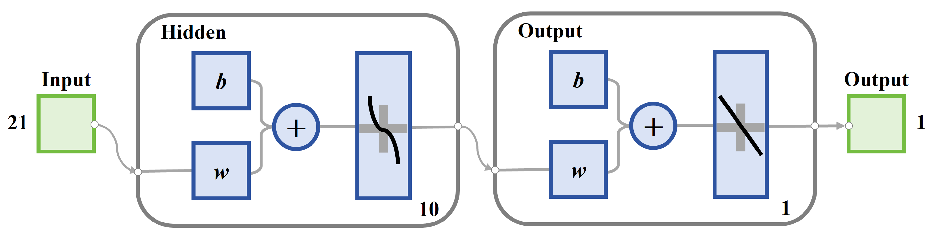
2.2. Neural Network Design and Hyperparameter Setting

A fully connected neural network is a fundamental neural network model in which each neuron in one layer is connected to every neuron in the next layer. This network architecture can effectively capture the complex nonlinear relationships between input features and outputs [31]. The TRAINLM (Levenberg–Marquardt) backpropagation algorithm is an optimization algorithm used for training artificial neural networks, combining the advantages of gradient descent and Newton’s method. It is particularly suitable for small- to medium-sized networks and can converge to the optimal solution more quickly [32]. This paper integrates the fully connected artificial neural network with the faster-converging TRAINLM backpropagation algorithm to learn the relationship between input data and output elevation values from the training data, thereby achieving integrated elevation prediction.
In the neural network fusion task, after addressing the preparation and cleaning of the training data, the input and output layers are determined. The remaining undetermined aspects are the number of hidden layers and the number of neurons, which need to be specifically determined through experiments. In the experiments, 70% of the training data are used for training, 15% for validation to control the training process and avoid overfitting and underfitting, and the entire proposed framework is implemented on an independent dataset. The network parameters, such as the depth of each layer and the number of neurons, are adjusted, with the remaining 15% of the data used to monitor the neural network’s performance during training. To select the optimal number of hidden layers and neurons, repeated experiments were conducted. Ultimately, a structure with one hidden layer and ten neurons was chosen for a balance between efficiency and effectiveness. The selection of the neural network structure is based on specific criteria. Firstly, the focus of this paper is on the application of neighboring elevation and curvature features rather than on the number of neurons within the network. For the relatively straightforward fitting task in this experiment, the number of hidden layers does not significantly affect the fusion results. Secondly, the number of neurons in an artificial neural network is a crucial parameter of the network’s architecture. Typically, the neural network structure is predetermined based on prior experience from existing studies or extensive testing.
Figure 4 illustrates the neural network architecture determined in the experiment, including the input layer, hidden layer, and output layer. The input layer consists of 21 input features, represented by green squares. These input features are passed to the hidden layer, which is composed of 10 neurons. Each input feature is connected to the hidden-layer neurons through weights (w) and biases (b), denoted as w and b in the diagram and indicated by plus symbols. The weighted sum is transformed by an activation function, shown as black curves in the Figure 4. The output layer consists of 1 neuron, receiving input from the hidden layer. Similarly, the hidden layer’s output is connected to the output neuron through weights and biases, marked by w and b and plus symbols. The output layer’s weighted sum is also transformed by an activation function, depicted by black curves.

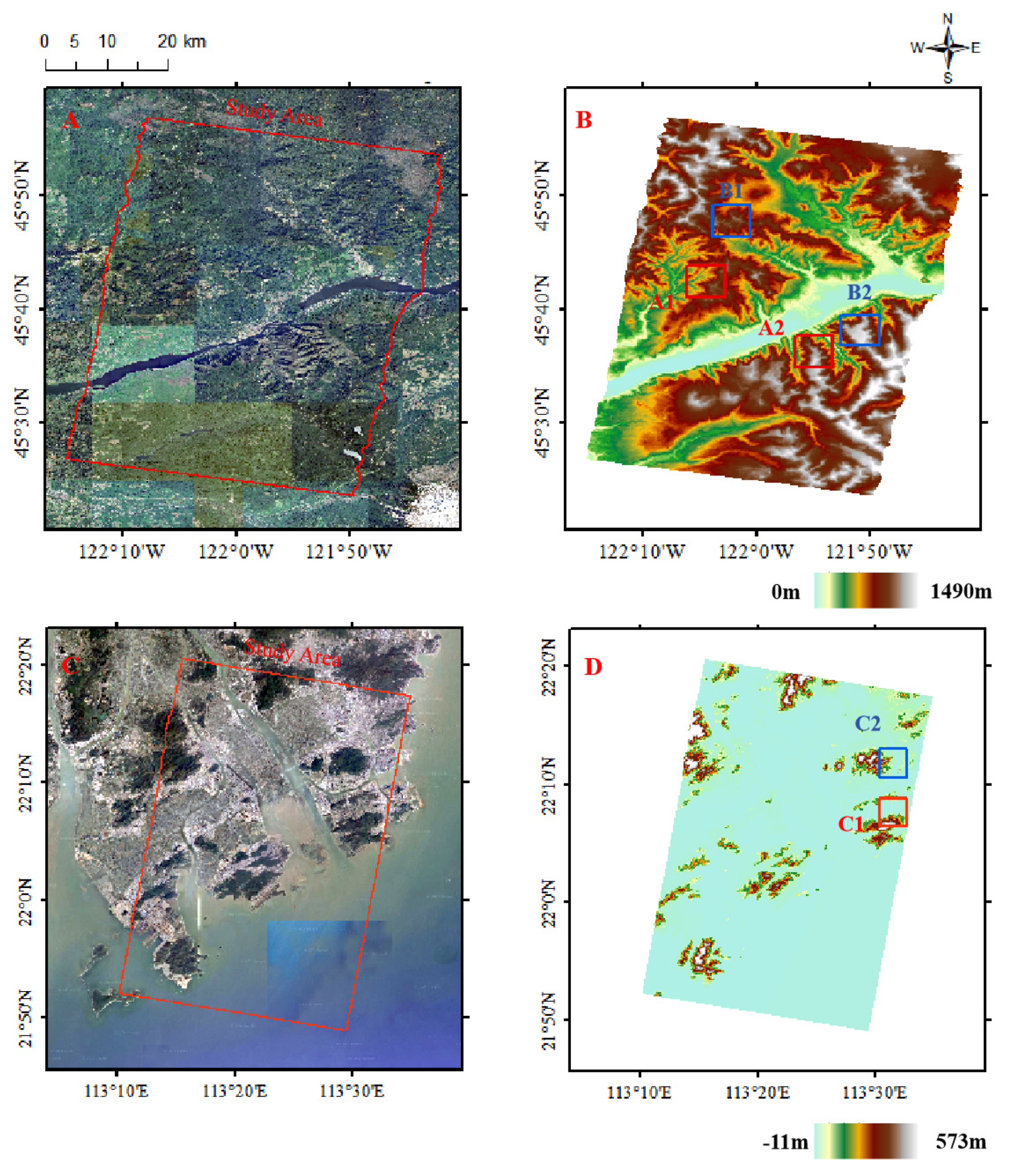
2.3. Study Area and Experimental Data

This section of the experiment selects the Oregon Experimental Area in the United States, which is a typical mountainous region with significant elevation variations and relatively low DEM accuracy, presenting an opportunity and need for quality improvement. In addition, we added the Macao region as another experimental area, and the urban area has serious occlusion and still has the problem of low data quality. The optical basemaps are sourced from Google Earth in Figure 5A,C. The InSAR−DEM experimental data come from TanDEM-X interferometric data processing and have undergone void filling [33]. The optical DEM is sourced from the publicly available AW3D30 DEM, with a resolution of 30 m and an absolute elevation accuracy better than 5 m. It is one of the higher-accuracy optical DEMs available in global public datasets, so the impact on accuracy after resampling can be minimized [34]. The AW3D30 DEM was resampled to ensure that the resolutions of the InSAR and optical DEM fusion were consistent. Verification data are sourced from LiDAR data in the US 3DEP program, with a resolution of 10 m and an absolute elevation accuracy better than 1 m. By standardizing the InSAR−DEM, AW3D30 DEM, and LiDAR DEM to the same reference system, both datasets are based on the same reference framework.
Research indicates that for shallow neural networks, a smaller dataset can produce stable prediction results, while excessively large and noisy datasets can obscure the regression relationships in the training data. Bagheri et al. [10] found in their experiments that 2000 sample points are sufficient for a neural network with 20 neurons to achieve stable prediction results. Therefore, not all elevation points in the dataset are used for training and testing. In this paper, a training sample size of 500 × 500 is deemed sufficient. Terrain selection is crucial as mountain height and variability can affect the accuracy of InSAR and optical DEMs to different extents, leading to different error patterns. Training and prediction based on varying terrain conditions is a more prudent approach. This paper primarily addresses the quality enhancement of DEMs in mountainous and urban areas, so the selected data do not include flat and hilly terrains. Finally, training and prediction areas are selected separately for high- and low-mountain terrains and urban areas, with specific locations indicated in Figure 5 and the details of the training and test sets for different data sources shown in Figure 6. Table 1 shows the details of the experimental data.

3. Results

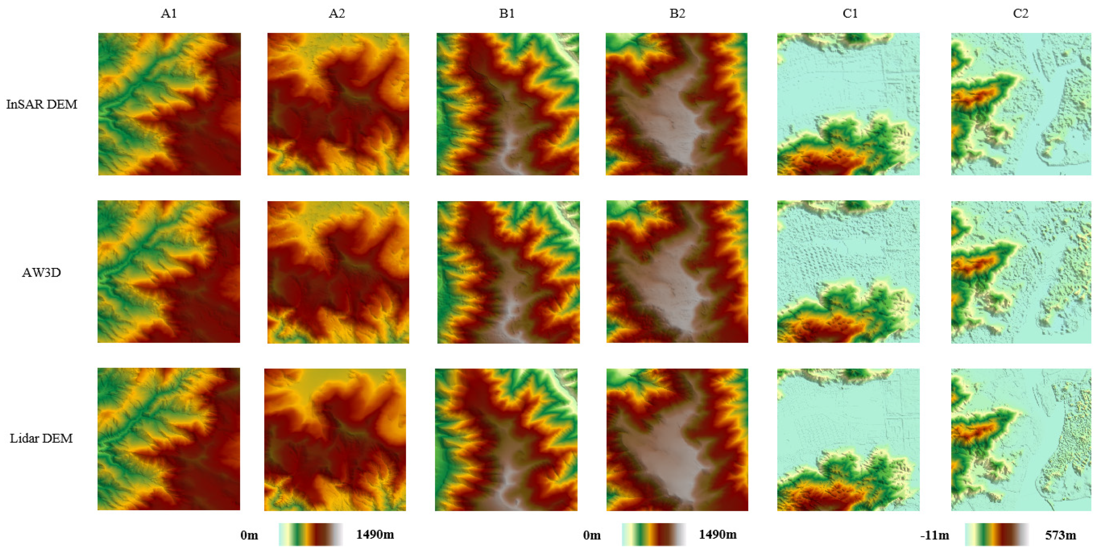
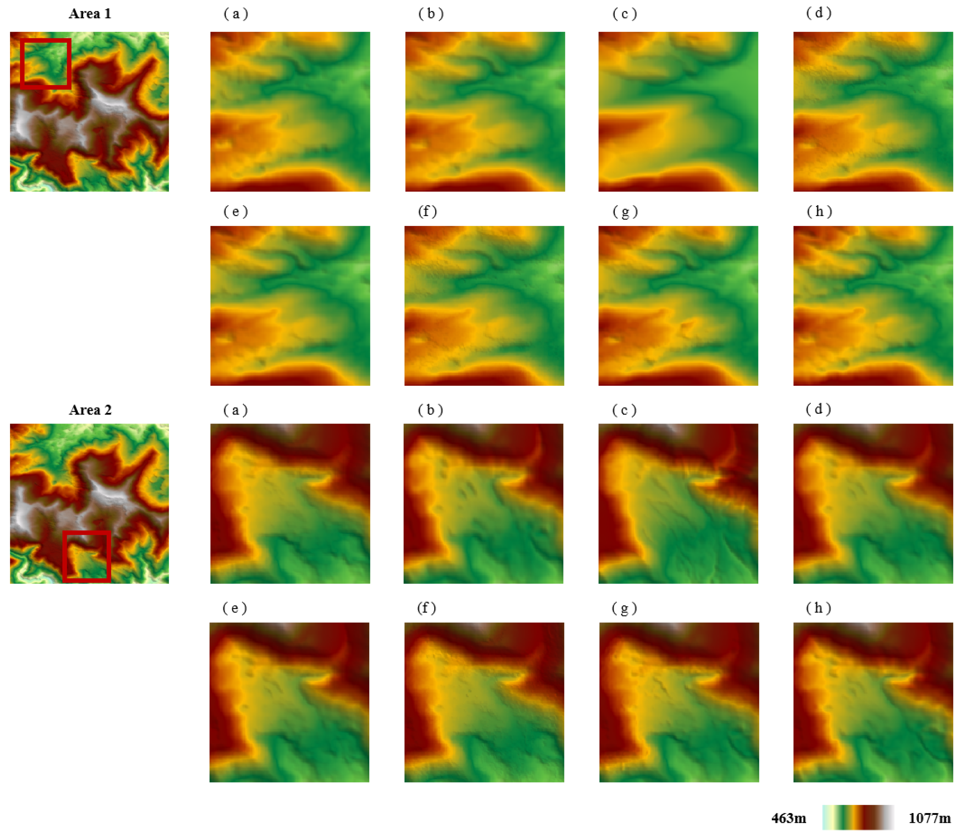
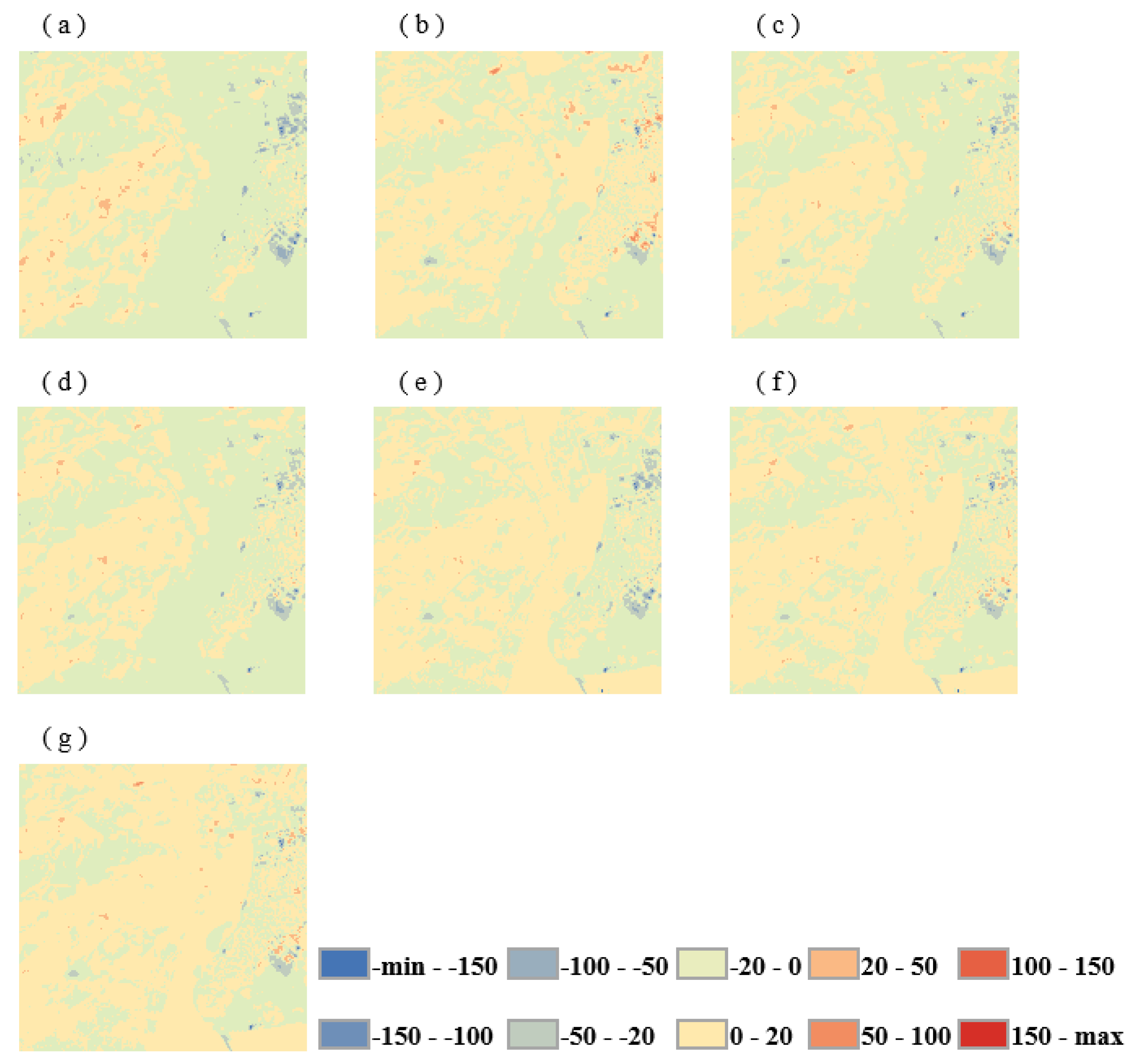
3.1. DEM Fusion Results via Different Methods

Based on the aforementioned experimental conditions, this paper conducts a fusion study of InSAR and optical DEMs. To demonstrate the effectiveness of the proposed method, three sets of control experiments were conducted. The first set is a simple averaging method, which is easy to implement and provides some improvement. The second set is an adaptive weighted averaging method, which can obtain complementary information from different DEMs and has noise resistance capabilities. The third set is a neural network fusion method that uses only terrain information as input, with network parameters designed to be consistent with the proposed method. The aim is to explore the impact of terrain features and surrounding elevations on the fused DEM.
In Figure 7 and Figure 8, the fusion results of the A2 and B2 regions are shown. Visually, the results of the fusion method proposed in this study do not show significant differences compared to other existing fusion methods. In fact, the fusion results show only minor differences compared to the input InSAR and optical DEMs. The main reason for this is that the elevation range of the DEM data selected for the experiment is very large, close to 1000 m. In such a large elevation range, the vertical elevation change of the DEM before and after fusion is usually only a few tens of meters, which makes it difficult to visually observe significant differences in the rendered DEM image. However, in Figure 9, within the C2 region, where the elevation range is relatively small, the differences become noticeably apparent after fusion.
However, this does not mean that the results of the experiment are not valuable or effective. On the contrary, the significance of this result lies in the fact that the proposed network-based fusion method can ensure the overall stability of the generated DEM while maintaining the overall terrain characteristics. In other words, this method does not lead to a change in the terrain characteristics, indicating its applicability and stability in different terrain conditions. At the same time, this stability also proves that the fusion method is consistent in the processing of different data sources, and can effectively retain the characteristics of the original terrain without introducing significant errors or biases. Therefore, the contribution of this study is to validate a new fusion method that is not only theoretically feasible, but also shows good stability and consistency in practical applications.

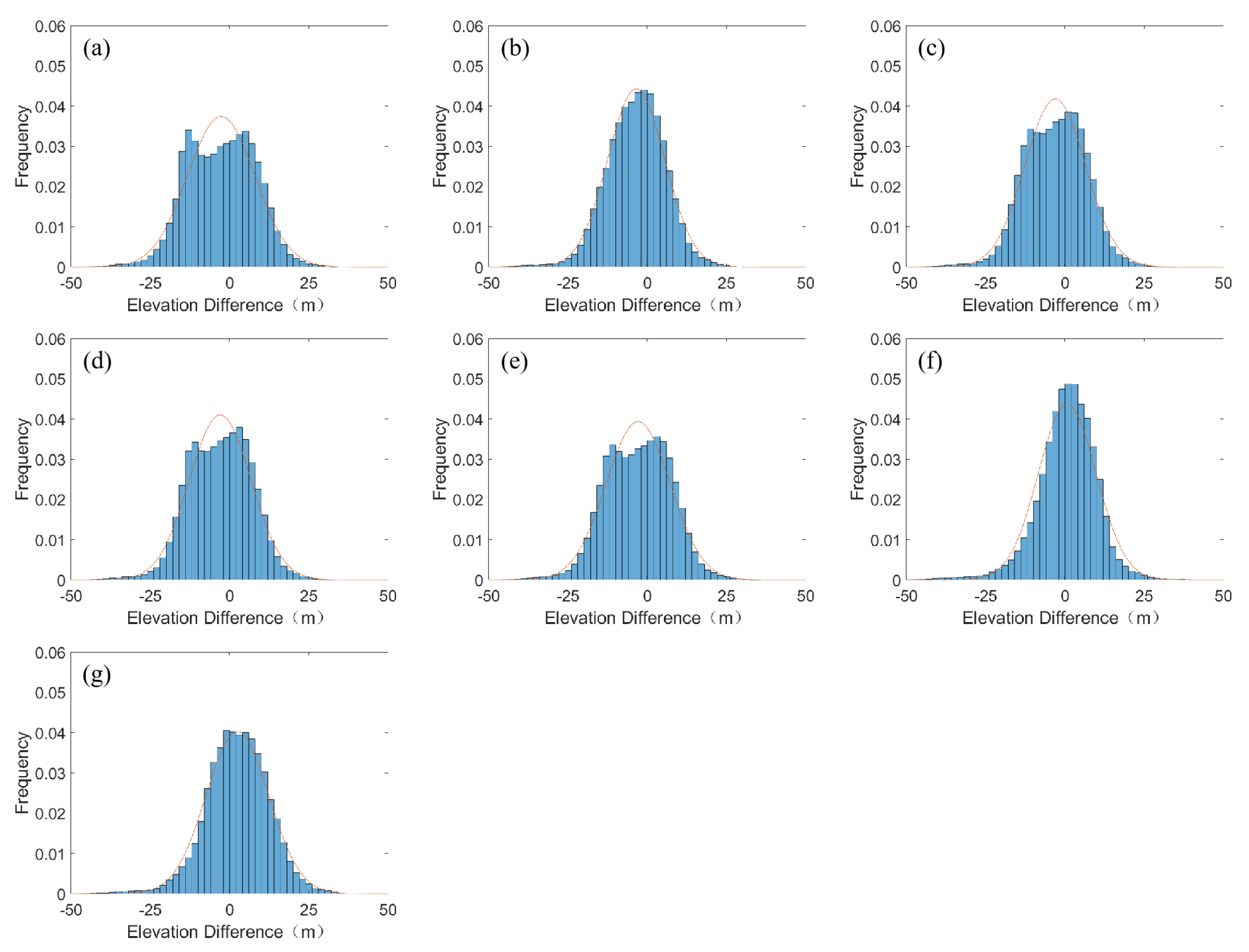
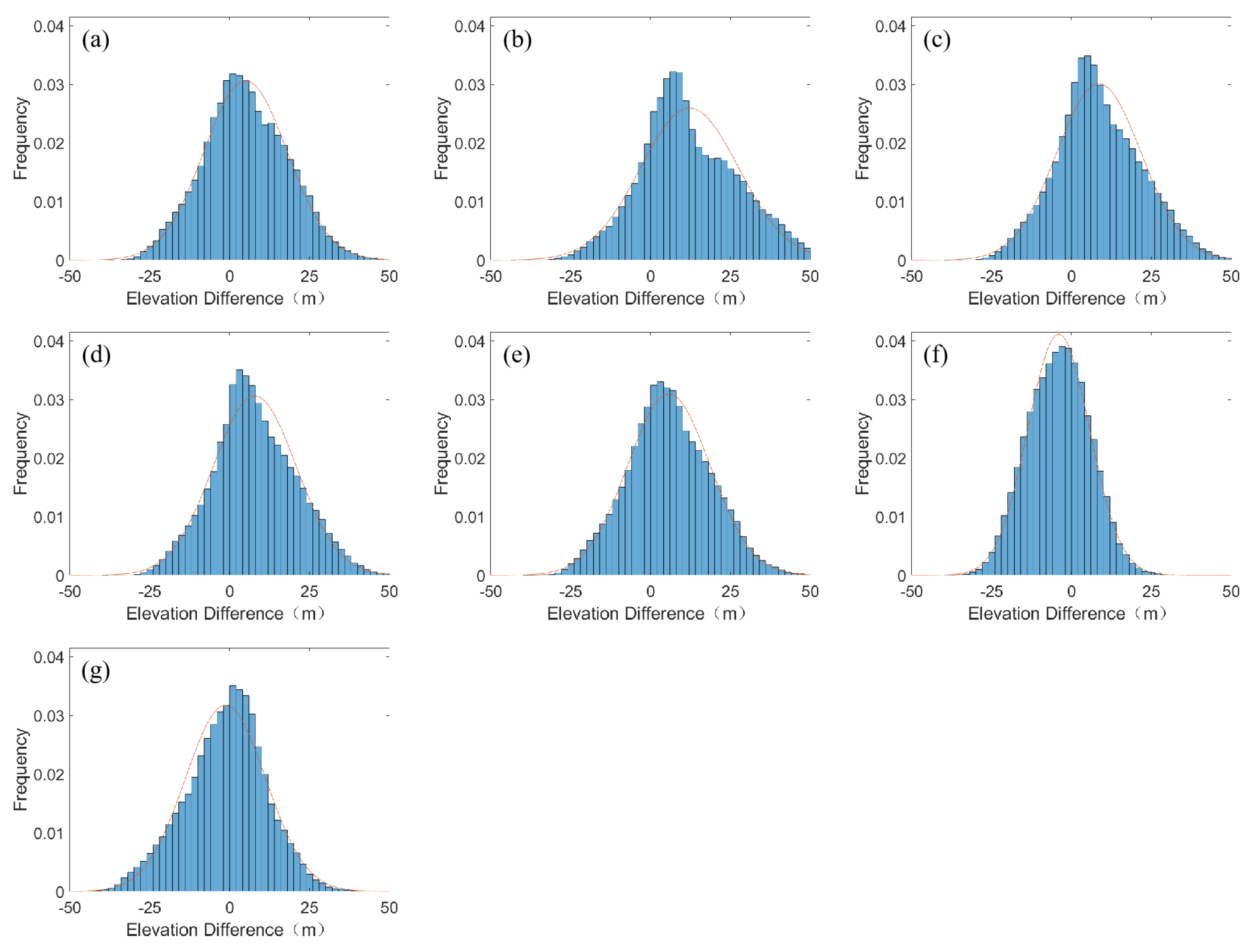
3.2. Elevation Difference Analysis

To analyze the DEMs, we calculate the difference between the DEMs under study and the reference DEM to obtain error distribution maps. These difference maps are then categorized to visually represent the characteristics of the error variations. Errors of different magnitudes are represented with varying color intensities, with deeper colors indicating larger errors. Figure 10, Figure 11 and Figure 12 illustrate the error spatial distribution maps for the InSAR−DEM, AW3D30 DEM, and the DEMs obtained through five different fusion methods. These maps facilitate a further analysis of the quality of the DEM results before and after fusion, as well as among different fusion methods.
From the spatial distribution of the difference maps between InSAR and AW3D30 DEMs, most of the absolute errors are concentrated within 20 m. The DEM obtained by simple averaging fusion shows minimal change in error compared to the original DEM, with performance lying between that of InSAR and AW3D30 DEMs. The DEM fused using the adaptive regularization variational model shows a significant reduction in error levels, and the DEM fused using only terrain inputs from the neural network further reduces error levels. Various fusion methods can mitigate the impact of errors to some extent through information complementarity, improving the DEM accuracy. The neural network fusion DEM, considering terrain features, achieves the least dark color distribution in both low-mountain and high-mountain areas, indicating the smallest magnitude of error. Among all fusion methods, it is closest to the true terrain, with a more noticeable improvement in the high-mountain area compared to the low-mountain area, achieving the smallest error level. This is primarily due to two factors: firstly, the neural network-based fusion method can learn the relationship between the coarse input terrain and the desired precise terrain; secondly, the inclusion of terrain curvature and surrounding elevations in this paper provides a solid basis for this relationship, resulting in better high-precision DEM mapping. Experiments in both low-mountain and high-mountain areas show that in more complex terrain, the original InSAR and AW3D30 DEMs have lower accuracy, thus providing greater potential for accuracy improvement. A well-tuned neural network can demonstrate a higher capacity for accuracy enhancement.
Table 2 shows the statistical results of the DEM accuracy assessment based on InSAR and optical DEM fusion methods. The statistical metrics used are RMSE, reflecting overall error size, and NMAD, which is robust to outliers and thus reflects the error after removing gross errors; smaller values indicate higher DEM accuracy. The simple averaging fusion results in accuracy between InSAR and AW3D30 DEMs. The adaptive regularization variational model fusion DEM shows a slight increase in NMAD value in high-mountain areas, with RMSE slightly lower than InSAR−DEM. In low-mountain areas, the accuracy also lies between InSAR and AW3D30 DEMs. This may be because the original DEMs have a resolution difference of three times, limiting the model’s ability to extract complementary information. The neural network fusion with only terrain inputs shows improved accuracy in high-mountain areas but lower accuracy than AW3D30 DEM in low-mountain areas. This indicates that while the neural network can improve fusion DEM accuracy, the lower range of errors in the low-mountain area limits further improvement, suggesting a need for additional input information to learn deeper error relationships. Compared to the DEM with the highest accuracy among the input DEMs, the neural network fusion DEM considering local terrain shows an increase in RMSE by 18.3%, 3.7%, and 9.4% in high- and low-mountain areas, respectively, and an increase in NMAD by 20.6%, 10.3%, and 26.6% in high- and low-mountain areas and urban landscapes, respectively.
Figure 13, Figure 14 and Figure 15 show histograms of error distributions for the quantitative evaluation metrics, indicating the distribution of errors in terms of magnitude; the red curve represents the probability distribution curve of the error fitting. The DEMs obtained through the proposed fusion method exhibit errors that are more tightly clustered around zero, closely approximating a normal distribution. This demonstrates the stability of the predictions and the superiority of the proposed method compared to others. Combined with the error spatial distribution maps and quantitative statistical indicators, consistent conclusions can be drawn. The proposed method achieves the highest fusion accuracy in all types of terrain, indicating that the neural network fusion method, which considers terrain features, can fully utilize the existing InSAR and optical DEM data. It enhances the quality of DEM data without additional costs and effectively improves the quality of single-source DEM data in mountainous areas.

4. Discussion

4.1. Effects of Neural Network Hyperparameters and Window Size

To determine the impact of hyperparameter settings and the neighboring elevation window size on experimental results in artificial neural networks (ANNs), a series of comparative experiments were conducted. The inclusion of neighboring elevation inputs provides additional information without relying on external data, particularly reflecting the correlation of elevation values among adjacent pixels. The choice of neighboring window size also significantly affects the information acquisition process. Thus, four sets of comparative experiments were conducted with window sizes of 3 × 3, 5 × 5, 7 × 7, and 9 × 9 to investigate the impact of window size on the results. All other experimental conditions remained the same, and the accuracy assessment results are shown in Table 3. In high-mountain areas, low-mountain areas, and urban areas, the 3 × 3 window consistently demonstrated superior performance. Therefore, the 3 × 3 window was selected for obtaining neighboring elevation data for further experimentation.
Additionally, the number of hidden layers and neurons per layer are crucial parameters in the neural network structure. The impact of different network structures on the fusion effect was also explored. The results in Table 4 indicated that changes in the network structure do not necessarily lead to greater improvements in the DEM fusion process with increased network complexity. However, a more complex network results in longer training times. Considering both the impact of network structure on fusion effectiveness and training efficiency, a network with one hidden layer containing 10 neurons was chosen for the experiments.

4.2. Verification of Curvature Characteristics and Surrounding Elevations

In this section, the impact of curvature and surrounding elevation on our method is discussed. To reveal the influence of the local topography, four additional experiments, including different combinations of slope, aspect, curvature, and surrounding elevation, were conducted, where we controlled the input DEM and reference DEM, the number of network layers and neurons, and training hyperparameters, ensuring their uniformity across all configurations. The accuracy statistics RMSE (Root-Mean-Squared Error) and NMAD (Normalized Median Absolute Deviation) were used to reflect the fusion performance, and the results are listed in Table 3. The inclusion of slope and aspect improves the accuracy of DEM fusion, particularly reducing the NMAD metric significantly. This indicates that terrain features help to lower the overall noise level of the DEM. Furthermore, the curvature is the second derivative of the terrain, providing information distinct from first-order derivatives such as slope and aspect. The integration of curvature leads to a notable improvement in the fusion performance, which validates the effectiveness of curvature.
Additionally, an additional comparison experiment considering only surrounding elevation was incorporated into the study. The fusion results incorporating surrounding elevation show a significant enhancement over the results based solely on DEM, which established the imperative of incorporating surrounding elevation as crucial input data. Finally, training was performed using inputs that included slope, aspect, curvature, and surrounding elevation features, which yielded the best fusion results. Our proposed method exhibited the optimal performance in this series of experiments, proving to be the most suitable for InSAR DEM and optical satellite-derived DEM. However, it is worth noting that, compared to the results in Table 5, the improvement in fusion accuracy with different input features is relatively modest. The similarity between test data from different regions and the training data is not the same; in this section, the data similarity is notably lower compared to previous experiments, resulting in a much smaller improvement in accuracy. This limitation is one of the main constraints of this study. Figure 16 illustrates the regression relationship between training and prediction in the fifth experimental group. The vertical axis represents the fusion results output by the neural network, while the horizontal axis denotes the elevation data points used for training, specifically the Lidar DEM data. In the title, R indicates the correlation between the output results and the target. It is evident that there is a notably robust association between the input elevation and the predicted elevation.

4.3. Suitable Situations and Future Improvement Directions of the Proposed Method

Since the datasets used in our paper are sourced from the same geographical region, which exhibits rather uniform topographic structures and geomorphological features, the transferability of the proposed method is limited. Topographic data involve complex characteristics. Although we categorized the data into high-mountain areas and low-mountain areas for training and testing, achieving effective application in the diverse and intricate topographic configurations remains difficult. Therefore, future work should focus on constructing DEM fusion sample sets for different types of landforms. Furthermore, the neural network architecture employed in this paper is relatively simplistic, which constrains its feature extraction capabilities in complex terrain conditions. Deep learning possesses robust capabilities in feature representation, which mines potential spatial patterns from terrain data. The network model can establish elevation residual models for various landforms through extensive learning, thereby facilitating the fusion of InSAR DEM and optical satellite-derived DEM across a broader range of applications and scenarios.

5. Conclusions

The combined use of InSAR and optical DEMs is anticipated to significantly enhance DEM data quality with minimal additional cost. This paper builds on the analysis of existing InSAR and optical DEM fusion methods, revealing the crucial role of local elevation and curvature features in improving fusion outcomes. Consequently, an enhanced artificial neural network (ANN) framework for DEM fusion has been proposed, incorporating local elevation and curvature features as input variables. The discussion demonstrates that the additional accuracy improvements in DEMs are attributable to these two input features. Experiments conducted in an experimental area in Oregon, USA, show that the improved fusion framework significantly enhances DEM fusion accuracy. Compared to simple averaging and adaptive regularization variational models, the fused DEM generated by the proposed method exhibits the lowest Root-Mean-Squared Error (RMSE) and Normalized Median Absolute Deviation (NMAD) values. Error analysis indicates that this method effectively reduces errors due to terrain undulations, with the fused DEM approaching a normal distribution. Compared to the original DEM, RMSE values improve by 5.0% to 12.3%, and NMAD values improve by 10.3% to 20.6%, thereby demonstrating the reliability of the proposed framework.
However, it is important to note that the proposed framework has certain limitations in its application. The enhancement of fusion results depends on the similarity between training and test data, requiring good terrain distribution similarity between these datasets. This is due to the core of neural network learning being the mapping relationship between terrain and elevation. Improving the applicability of the DEM fusion framework is a significant challenge and an ongoing area of effort. In future work, we aim to extend the fusion framework from artificial neural networks to deep neural networks, with the goal of enhancing its ability to adapt to diverse terrains and landforms, thereby increasing its practical significance.

Author Contributions

Conceptualization, R.G., Q.S. and Z.H.; methodology, R.G. and J.H.; software, R.G. and Q.S.; validation, R.G., Y.Q. and J.H.; formal analysis, R.G., Z.H. and Y.Q.; investigation, Y.Y., J.D. and Z.M.; resources, R.G., J.H. and Q.S.; data curation, R.G., Q.S. and J.H.; writing—original draft preparation, R.G., Y.Q. and Z.M.; writing—review and editing, all authors; visualization, Q.S., Y.Y. and Y.Q.; supervision, R.G., Q.S. and J.H.; project administration, R.G. and J.H.; funding acquisition, R.G. and J.H. All authors have read and agreed to the published version of the manuscript.

Funding

This work was supported by the National Natural Science Foundation of China under grants 42201432, 42474054 and 42030112, the science and technology innovation program of Hunan Province (No. 2022RC3042), and the science and technology innovation program of Fujian Province (No. 2021Y3001).

Data Availability Statement

Data are contained within the article.

Acknowledgments

The authors would like to thank DLR for providing the TanDEM-X data and USGS for providing the LiDAR DEM (U.S. Geological Survey, 2023, 1/3rd arc-second Digital Elevation Models (DEMs)–USGS National Map 3DEP Downloadable Data Collection: U.S. Geological Survey). The authors would like to thank the editor, associate editor, and anonymous reviewers for their constructive and helpful comments that greatly improved this article.

Conflicts of Interest

The authors declare no conflicts of interest.

References

  1. Song, H.; Jung, J. An object-based ground filtering of airborne lidar data for large-area dtm generation. Remote Sens. 2023, 15, 4105. [Google Scholar] [CrossRef]
  2. Hoja, D.; Reinartz, P.; Schroeder, M. Comparison of DEM generation and combination methods using high resolution optical stereo imagery and interferometric SAR data. Rev. Française Photogrammétrie Télédétection 2007, 2006, 89–94. [Google Scholar]
  3. Schmitt, M.; Zhu, X.X. Data fusion and remote sensing: An ever-growing relationship. IEEE Geosci. Remote Sens. Mag. 2016, 4, 6–23. [Google Scholar] [CrossRef]
  4. Banu, R.S. Medical Image Fusion by the analysis of Pixel LevelMulti-sensor Using Discrete Wavelet Transform. In Proceedings of the National Conference on Emerging Trends in Computing Science, Shillong, India, 4–5 March 2011; pp. 291–297. [Google Scholar]
  5. Leitão, J.; De Sousa, L. Towards the optimal fusion of high-resolution Digital Elevation Models for detailed urban flood assessment. J. Hydrol. 2018, 561, 651–661. [Google Scholar] [CrossRef]
  6. Gruber, A.; Wessel, B.; Martone, M.; Roth, A. The TanDEM-X DEM mosaicking: Fusion of multiple acquisitions using InSAR quality parameters. IEEE J. Sel. Top. Appl. Earth Obs. Remote Sens. 2015, 9, 1047–1057. [Google Scholar] [CrossRef]
  7. Deo, R.; Rossi, C.; Eineder, M.; Fritz, T.; Rao, Y. Framework for fusion of ascending and descending pass TanDEM-X raw DEMs. IEEE J. Sel. Top. Appl. Earth Obs. Remote Sens. 2015, 8, 3347–3355. [Google Scholar] [CrossRef]
  8. Tran, T.; Raghavan, V.; Masumoto, S.; Vinayaraj, P.; Yonezawa, G. A geomorphology-based approach for digital elevation model fusion–case study in Danang city, Vietnam. Earth Surf. Dyn. 2014, 2, 403–417. [Google Scholar] [CrossRef]
  9. Schindler, K.; Papasaika-Hanusch, H.; Schütz, S.; Baltsavias, E. Improving wide-area DEMs through data fusion-chances and limits. In Proceedings of the Photogrammetric Week, Stuttgart, Germany, 1–4 April 2011; pp. 159–170. [Google Scholar]
  10. Bagheri, H.; Schmitt, M.; Zhu, X.X. Fusion of TanDEM-X and Cartosat-1 elevation data supported by neural network-predicted weight maps. ISPRS J. Photogramm. Remote Sens. 2018, 144, 285–297. [Google Scholar] [CrossRef]
  11. Wang, W.; Zhang, C.; Ng, M.K. Variational model for simultaneously image denoising and contrast enhancement. Opt. Express 2020, 28, 18751–18777. [Google Scholar] [CrossRef]
  12. Kuschk, G.; d’Angelo, P.; Gaudrie, D.; Reinartz, P.; Cremers, D. Spatially regularized fusion of multiresolution digital surface models. IEEE Trans. Geosci. Remote Sens. 2016, 55, 1477–1488. [Google Scholar] [CrossRef]
  13. Bagheri, H.; Schmitt, M.; Zhu, X.X. Fusion of TanDEM-X and Cartosat-1 DEMs using TV-norm regularization and ANN-predicted weights. In Proceedings of the 2017 IEEE International Geoscience and Remote Sensing Symposium (IGARSS), Fort Worth, TX, USA, 23–28 July 2017; pp. 3369–3372. [Google Scholar]
  14. Guan, L.; Hu, J.; Pan, H.; Wu, W.; Sun, Q.; Chen, S.; Fan, H. Fusion of public DEMs based on sparse representation and adaptive regularization variation model. ISPRS J. Photogramm. Remote Sens. 2020, 169, 125–134. [Google Scholar] [CrossRef]
  15. Slatton, K.C.; Crawford, M.; Teng, L. Multiscale fusion of INSAR data for improved topographic mapping. In Proceedings of the IEEE International Geoscience and Remote Sensing Symposium, Toronto, ON, Canada, 24–28 June 2002; pp. 69–71. [Google Scholar]
  16. Zhang, S.; Foerster, S.; Medeiros, P.; de Araújo, J.C.; Motagh, M.; Waske, B. Bathymetric survey of water reservoirs in north-eastern Brazil based on TanDEM-X satellite data. Sci. Total Environ. 2016, 571, 575–593. [Google Scholar] [CrossRef] [PubMed]
  17. Tang, Y.; Atkinson, P.M.; Zhang, J. Downscaling remotely sensed imagery using area-to-point cokriging and multiple-point geostatistical simulation. ISPRS J. Photogramm. Remote Sens. 2015, 101, 174–185. [Google Scholar] [CrossRef]
  18. Sadeq, H.; Drummond, J.; Li, Z. Merging digital surface models implementing Bayesian approaches. Int. Arch. Photogramm. Remote Sens. Spat. Inf. Sci. 2016, 41, 711–718. [Google Scholar] [CrossRef]
  19. Jiang, H.; Zhang, L.; Wang, Y.; Liao, M. Fusion of high-resolution DEMs derived from COSMO-SkyMed and TerraSAR-X InSAR datasets. J. Geod. 2014, 88, 587–599. [Google Scholar] [CrossRef]
  20. Fuss, C.E.; Berg, A.A.; Lindsay, J.B. DEM Fusion using a modified k-means clustering algorithm. Int. J. Digit. Earth 2016, 9, 1242–1255. [Google Scholar] [CrossRef]
  21. Girohi, P.; Bhardwaj, A. ANN-Based DEM Fusion and DEM Improvement Frameworks in Regions of Assam and Meghalaya using Remote Sensing Datasets. Eur. J. Environ. Earth Sci. 2022, 3, 79–89. [Google Scholar] [CrossRef]
  22. Girohi, P.; Bhardwaj, A. A Neural Network-Based Fusion Approach for Improvement of SAR Interferometry-Based Digital Elevation Models in Plain and Hilly Regions of India. AI 2022, 3, 820–843. [Google Scholar] [CrossRef]
  23. Valiante, M.; Di Benedetto, A.; Aloia, A. A Comparison of Landforms and Processes Detection Using Multisource Remote Sensing Data: The Case Study of the Palinuro Pine Grove (Cilento, Vallo di Diano and Alburni National Park, Southern Italy). Remote Sens. 2024, 16, 2771. [Google Scholar] [CrossRef]
  24. Carlisle, B.H. Modelling the spatial distribution of DEM error. Trans. GIS 2005, 9, 521–540. [Google Scholar] [CrossRef]
  25. Aguilar, F.J.; Agüera, F.; Aguilar, M.A.; Carvajal, F. Effects of terrain morphology, sampling density, and interpolation methods on grid DEM accuracy. Photogramm. Eng. Remote Sens. 2005, 71, 805–816. [Google Scholar] [CrossRef]
  26. Arun, P.V. A comparative analysis of different DEM interpolation methods. Egypt. J. Remote Sens. Space Sci. 2013, 16, 133–139. [Google Scholar]
  27. Heritage, G.L.; Milan, D.J.; Large, A.R.; Fuller, I.C. Influence of survey strategy and interpolation model on DEM quality. Geomorphology 2009, 112, 334–344. [Google Scholar] [CrossRef]
  28. Guth, P.; Kane, M. Slope, aspect, and hillshade algorithms for non-square digital elevation models. Trans. GIS 2021, 25, 2309–2332. [Google Scholar] [CrossRef]
  29. Wilson, J.P. Digital terrain modeling. Geomorphology 2012, 137, 107–121. [Google Scholar] [CrossRef]
  30. Höhle, J.; Höhle, M. Accuracy assessment of digital elevation models by means of robust statistical methods. ISPRS J. Photogramm. Remote Sens. 2009, 64, 398–406. [Google Scholar] [CrossRef]
  31. Cong, S.; Zhou, Y. A review of convolutional neural network architectures and their optimizations. Artif. Intell. Rev. 2023, 56, 1905–1969. [Google Scholar] [CrossRef]
  32. Kermani, B.G.; Schiffman, S.S.; Nagle, H.T. Performance of the Levenberg–Marquardt neural network training method in electronic nose applications. Sens. Actuators B Chem. 2005, 110, 13–22. [Google Scholar] [CrossRef]
  33. Hu, Z.; Gui, R.; Hu, J.; Fu, H.; Yuan, Y.; Jiang, K.; Liu, L. InSAR Digital Elevation Model Void-Filling Method Based on Incorporating Elevation Outlier Detection. Remote Sens. 2024, 16, 1452. [Google Scholar] [CrossRef]
  34. Altunel, A.O. Questioning the effects of raster-resampling and slope on the precision of TanDEM-X 90 m digital elevation model. Geocarto Int. 2021, 36, 2366–2382. [Google Scholar] [CrossRef]
Figure 1. Flowchart of the proposed method for neural network-based fusion of InSAR DEM and optical satellite-derived DEM considering local terrain.
Remotesensing 16 03567 g001
Figure 2. Terrain feature maps extracted from training data: (ac) represent the slope, aspect, and curvature extracted from the DEM of the low-mountain region; (df) represent the slope, aspect, and curvature extracted from the DEM of the high-mountain region.
Remotesensing 16 03567 g002
Figure 3. Schematic diagram of a 3 × 3 window. Z1Z9, respectively, represent the elevation values of pixels within the window.
Remotesensing 16 03567 g003
Figure 4. The neural network architecture determined through the experiments. The input layer has a dimension of 21, the hidden layer contains 10 neurons, and the output layer has a dimension of 1. w represents the weights and b represents the biases.
Remotesensing 16 03567 g004
Figure 5. Illustration of the spatial split between intra-scene training data (red rectangular boxes A1, B1, and C1) and test data (blue rectangular boxes A2, B2, and C2). (A,C) are the optical basemaps of study areaes that sourced from Google Earth. (B,D) are the TanDEM-X data of Oregon, USA, and Macao, China.
Remotesensing 16 03567 g005
Figure 6. Training data and test data details.
Remotesensing 16 03567 g006
Figure 7. DEM fusion results for low-mountain areas (test data A2). (a) InSAR−DEM; (b) AW3D30; (c) reference DEM; (d) result of simple average fusion; (e) result of Maximum Likelihood Estimation; (f) result of Adaptive Regularization Variation Model; (g) result of terrain-based neural network; and (h) result of the proposed method.
Remotesensing 16 03567 g007
Figure 8. DEM fusion results for high-mountain areas (test data B2). (a) InSAR−DEM; (b) AW3D30; (c) reference DEM; (d) result of simple average fusion; (e) result of Maximum Likelihood Estimation; (f) result of Adaptive Regularization Variation Model; (g) result of terrain-based neural network; and (h) result of the proposed method.
Remotesensing 16 03567 g008
Figure 9. DEM fusion results for urban areas (rest data C2). (a) InSAR−DEM; (b) AW3D30; (c) reference DEM; (d) result of simple average fusion; (e) result of Maximum Likelihood Estimation; (f) result of Adaptive Regularization Variation Model; (g) result of terrain-based neural network; and (h) result of the proposed method.
Remotesensing 16 03567 g009
Figure 10. Error distribution for low-mountain areas (test data A2). (a) InSAR−DEM; (b) AW3D30; (c) result of simple average fusion; (d) result of Maximum Likelihood Estimation; (e) result of Adaptive Regularization Variation Model; (f) result of terrain-based neural network; and (g) result of the proposed method.
Remotesensing 16 03567 g010
Figure 11. Error distribution for high-mountain areas (test data B2). (a) InSAR−DEM; (b) AW3D30; (c) result of simple average fusion; (d) result of Maximum Likelihood Estimation; (e) result of Adaptive Regularization Variation Model; (f) result of terrain-based neural network; and (g) result of the proposed method.
Remotesensing 16 03567 g011
Figure 12. Error distribution for urban areas (test data C2). (a) InSAR−DEM; (b) AW3D30; (c) result of simple average fusion; (d) result of Maximum Likelihood Estimation; (e) result of Adaptive Regularization Variation Model; (f) result of terrain-based neural network; and (g) result of the proposed method.
Remotesensing 16 03567 g012
Figure 13. Error histogram for high-mountain areas (test data A2). (a) InSAR−DEM; (b) AW3D30; (c) result of simple average fusion; (d) result of Maximum Likelihood Estimation; (e) result of Adaptive Regularization Variation Model; (f) result of terrain-based neural network; and (g) result of the proposed method.
Remotesensing 16 03567 g013
Figure 14. Error histogram for high-mountain areas (test data B2). (a) InSAR−DEM; (b) AW3D30; (c) result of simple average fusion; (d) result of Maximum Likelihood Estimation; (e) result of Adaptive Regularization Variation Model; (f) result of terrain-based neural network; and (g) result of the proposed method.
Remotesensing 16 03567 g014
Figure 15. Error histogram for urban areas (test data C2). (a) InSAR−DEM; (b) AW3D30; (c) result of simple average fusion; (d) result of Maximum Likelihood Estimation; (e) result of Adaptive Regularization Variation Model; (f) result of terrain-based neural network; and (g) result of the proposed method.
Remotesensing 16 03567 g015
Figure 16. The regression relationship between training and prediction in the experimental portion of proposed method.
Remotesensing 16 03567 g016
Table 1. Detailed information about the prepared datasets.
Horizontal
Datum
Vertical
Datum
Resolution
(m)
Image Size
(Pixels)
InSAR−DEMWGS-84EGM08106043 × 4986
AW3D30 DEMWGS-84EGM96302019 × 2001
LiDAR DEMNAD83NAVD88106043 × 4986
A1, A2, B1, B2, C1, C2WGS-84EGM0810500 × 500
Fused DEMWGS-84EGM0810500 × 500
Table 2. Evaluation results of different methods.
High-Mountain Areas (A2)Low-Mountain Areas (B2)Urban Areas (C2)
RMSENMADRMSENMADRMSENMAD
InSAR−DEM13.8112.9410.9012.369.603.94
AW3D30 DEM19.0214.749.519.127.554.11
Simple Average Fusion15.3812.669.8510.457.443.62
Maximum Likelihood Estimation14.8712.4810.0110.827.743.69
Adaptive Regularization Variation Model13.9312.5310.4511.437.642.95
Terrain-based Neural Network13.2412.4910.199.607.203.15
Proposed11.2910.289.168.186.842.89
Table 3. Effect of adjacent elevation window on fusion result.
High-Mountain Areas/A1Low-Mountain Areas/B1Urban Areas/C1
RMSENMADRMSENMADRMSENMAD
3 × 311.069.799.178.506.842.89
5 × 511.149.659.458.766.932.99
7 × 711.239.689.658.5111.272.95
9 × 911.149.659.318.637.113.15
Table 4. Effect of neural network hyperparameters on fusion result.
High-Mountain Areas/A1Low-Mountain Areas/B1Urban Areas/C1
RMSENMADRMSENMADRMSENMADTime(s)
511.6310.7310.098.907.023.1486
1011.1810.259.368.416.843.20158
1511.2310.279.888.887.042.9252
2011.1910.279.988.946.962.93351
10-511.0010.3410.028.806.843.01212
15-811.1010.2810.309.106.933.19366
10-8-511.239.9610.148.896.893.23287
20-15-512.3210.1510.149.457.033.16744
Table 5. Evaluation fusion results on the effectiveness of curvature and surrounding elevation.
Input FeatureAccuracy
DEMSlope, AspectCurvatureSurrounding ElevationHigh-Mountain AreasLow-Mountain Areas
13.059.34
11.139.55
12.269.29
11.639.32
11.069.17
Disclaimer/Publisher’s Note: The statements, opinions and data contained in all publications are solely those of the individual author(s) and contributor(s) and not of MDPI and/or the editor(s). MDPI and/or the editor(s) disclaim responsibility for any injury to people or property resulting from any ideas, methods, instructions or products referred to in the content.

