Abstract
This study simulated the spatiotemporal changes in coastal ecosystem services (ESs) in the Jiaodong Peninsula from 2000 to 2050 and analyzed the driving mechanisms of climate change and human activities with respect to ESs, aiming to provide policy recommendations that promote regional sustainable development. Future climate change and land use were forecast based on scenarios from the Coupled Model Intercomparison Project Phase 6 (CMIP6). The Integrated Valuation of Ecosystem Services and Tradeoffs (InVEST) model was used to assess ESs such as water yield (WY), carbon storage (CS), soil retention (SR), and habitat quality (HQ). Key drivers of ESs were identified using Structural Equation Modeling (SEM). Results demonstrate the following: (1) High WY services are concentrated in coastal built-up areas, while high CS, HQ, and SR services are mainly found in the mountainous and hilly regions with extensive forests and grasslands. (2) By 2050, CS and HQ will show a gradual degradation trend, while the annual variations in WY and SR are closely related to precipitation. Among the different scenarios, the most severe ES degradation occurs under the SSP5-8.5 scenario, while the SSP1-2.6 scenario shows relatively less degradation. (3) SEM analysis indicates that urbanization leads to continuous declines in CS and HQ, with human activities and topographic factors controlling the spatial distribution of the four ESs. Climate factors can directly influence WY and SR, and their impact on ESs is stronger in scenarios with higher human activity intensity than in those with lower human activity intensity. (4) Considering the combined effects of human activities and climate change on ESs, we recommend that future development decisions be made to rationally control the intensity of human activities and give greater consideration to the impact of climate factors on ESs in the context of climate change.
1. Introduction
Over the past few decades, ecosystem services (ESs) have rapidly declined due to increased climate variability and intensified human activities [1,2]. Global warming has altered vegetation distribution [3] and terrestrial carbon cycles [4], interacting with land use changes to trigger widespread species extinction and migration [5,6]. Unsustainable land use has led to excessive greenhouse gas emissions [7], environmental pollution [8], and the shrinkage of wetlands [9] and lakes [10], further exacerbating irreversible ecosystem damage. Additionally, the increasing frequency and intensity of extreme weather events (such as heat waves [11], droughts [12], floods [13], and wildfires [14]), along with global public health crises like COVID-19 [15,16], underscore the widespread and profound risks associated with ongoing ecosystem degradation.
The Jiaodong Peninsula, located along China’s northern coast, is a critical region for economic growth and rapid urbanization. However, its ecosystems are under significant pressure and exhibit marked ecological sensitivity. Research suggests that climate change may reduce the suitable habitat for seagrass meadows, such as Zostera marina, by over 50% in this area [17]. Based on data from 1986 to 2015, Xia et al. reported that the ecosystems of the Jiaodong Peninsula are highly vulnerable to extreme climate events [18]. For example, severe droughts have significantly impacted agriculture and ecosystems during specific periods [19,20]. While coastal development and land reclamation have fueled regional economic growth, these human activities have exacerbated marine ecosystem degradation [21,22], increasing carbon emissions and environmental pollution [23,24,25], thereby directly threatening the region’s sustainable development. In this context, assessing the current ES status of the Jiaodong Peninsula, simulating its future distribution, and analyzing the driving mechanisms of climate change and human activities have become increasingly critical and urgent.
The Integrated Valuation of ES and Tradeoffs (InVEST) model has been integrated with land use simulation tools such as the Future Land Use Simulation (FLUS) and Patch-generating Land Use Simulation (PLUS) models and widely applied to forecast the spatial distribution of specific ESs [26,27,28]. In recent years, by incorporating Shared Socio-economic Pathways (SSPs) and Representative Concentration Pathways (RCPs) [29], the Coupled Model Intercomparison Project Phase 6 (CMIP6) has provided a comprehensive framework for predicting environmental changes under various future scenarios [30]. For example, Li et al. utilized the FLUS-InVEST framework within SSP-RCP scenarios to assess future ES changes in Central Asia [31]. Ji et al. analyzed and predicted habitat quality changes in the Yellow River Basin until 2050, integrating CMIP6 SSP-RCP scenarios with the PLUS model [32]. Guo et al. developed the LUH2-PLUS-InVEST framework to project future land use and carbon storage in China [33]. These studies help us better understand and address the dynamic changes in ESs under different climate contexts. However, some of studies primarily focus on terrestrial ecosystems and have yet to fully account for the local biases in GCM outputs from CMIP6. Moreover, in complex and fragmented landscapes such as coastal areas, a more precise inversion and calibration of land use data would enhance the accuracy of ES simulations [34].
As an ecologically sensitive coastal region, how have the historical conditions and future trends of key ESs in the Jiaodong Peninsula evolved under climate change and intensifying human activities? What are the key drivers behind these changes? Will the key drivers of ES changes evolve as climate change progresses? To enhance the accuracy of ES assessment results, this study optimized land classification data for the region and adjusted CMIP6 climate model predictions using observational data. Utilizing climate model data from CMIP6 SSP-RCP scenarios and land use simulation results, we assessed historical trends and forecasted future changes in the following four key ESs: water yield (WY), soil retention (SR), carbon storage (CS), and habitat quality (HQ). Structural equation modeling (SEM) was applied to unravel the complex factors driving these changes, providing a scientific foundation for policymakers to develop adaptive management strategies that foster sustainable development in the Jiaodong Peninsula.
2. Materials and Methods
2.1. Study Area
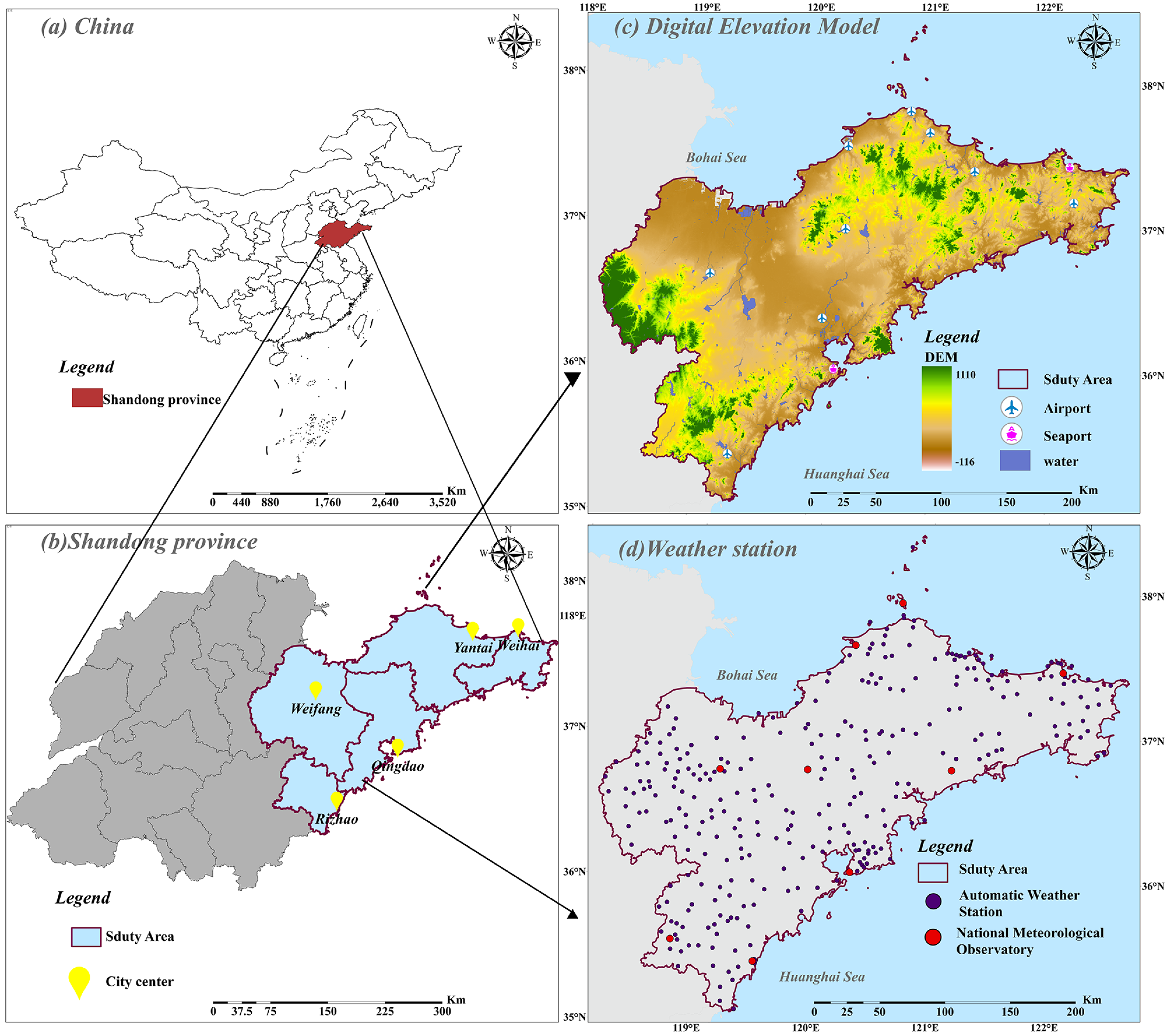
The Jiaodong Peninsula is located in Shandong Province in China’s eastern coastline region (118°10′–122°42′E, 35°04′–38°23′N), as shown in Figure 1. The peninsula is situated halfway between the Yellow and Bohai Seas and encompasses the coastal cities of Qingdao, Yantai, Weihai, Weifang, and Rizhao. The peninsula features low mountains and hills, predominantly in the northeastern and western parts; plains in the central and northern regions; and a typical mountainous bedrock bay-type coastline along the coastal areas. The Jiaodong Peninsula has a warm temperate monsoon climate with distinct maritime characteristics and is characterized by hot and rainy summers with concentrated precipitation that is difficult to retain, cold and dry winters, and frequent spring droughts. Between 2000 and 2020, the yearly average temperature varied from 12.1 to 13.7 °C, while the annual precipitation ranged from 489 to 947 mm.
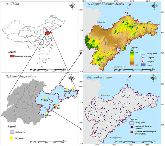
Figure 1.
Location of Jiaodong Peninsula.
The Jiaodong Peninsula spans roughly 52,000 square kilometers and has a population of approximately 32.43 million and a 67% urbanization rate. Qingdao, one of the cities in the Jiaodong Peninsula, is classified as a megacity, and Qingdao Port is the fourth largest port in China. The region’s agriculture and coastal economies are highly developed. Intense human activities and limited natural resources have led to fragile ecosystems, impacting the region’s long-term growth.
2.2. Sources of Data
The dataset employed in this study is composed of four categories: Satellite Imagery, Land Use Data, Climate Data, and Natural and Socio-economic Data. The detailed sources of each category are provided in Table 1.

Table 1.
List of the data used in this study.
2.3. Method
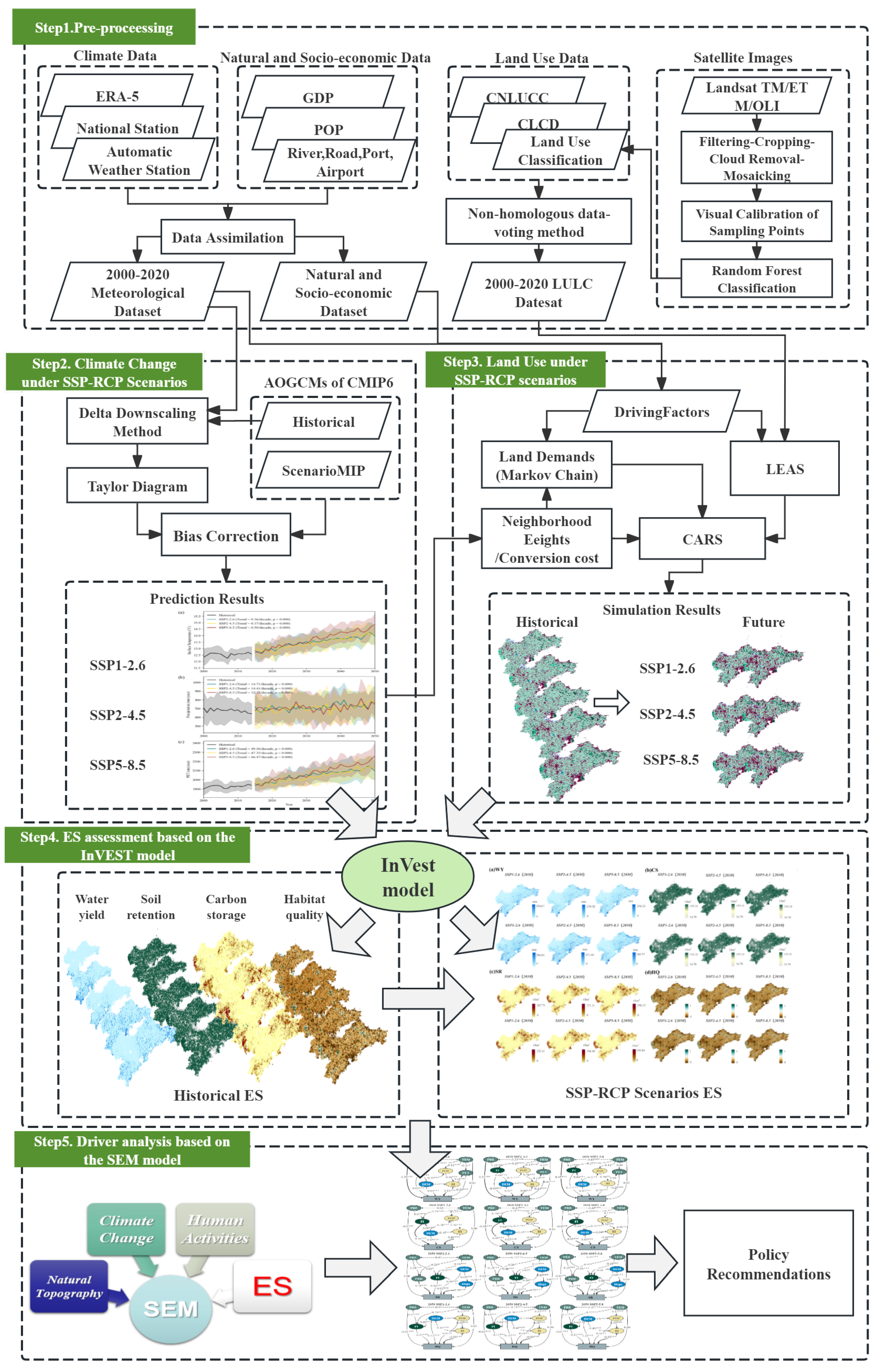
Figure 2 illustrates the research framework. It includes five modules: data preprocessing, climate change under SSP-RCP scenarios, land use under SSP-RCP scenarios, ES assessment based on the InVEST model, and driver analysis based on the SEM model.
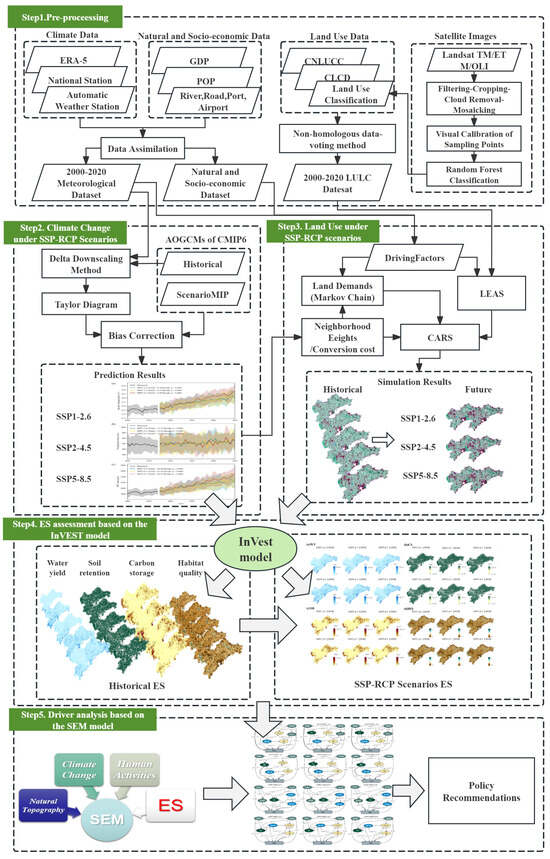
Figure 2.
CMIP6-PLUS-InVEST integrated ES assessment framework.
2.3.1. Data Preprocessing
Assimilation of Meteorological, Natural, and Socio-Economic Data
This study integrates data from various sources. To facilitate analysis and model calculations, meteorological data were assimilated into 1 km × 1 km grid data, while natural and socio-economic data were assimilated into 30 m × 30 m grid data to align with high-resolution satellite images. Bilinear interpolation was applied for gridded data, while kriging interpolation was applied for station data. OpenStreetMap data (transportation and rivers) were used to calculate distance metrics for the PLUS model’s driver analysis using the Raster Calculator in ArcGIS 10.8.
Land Use Reclassification Based on Non-Homogeneous Data Voting
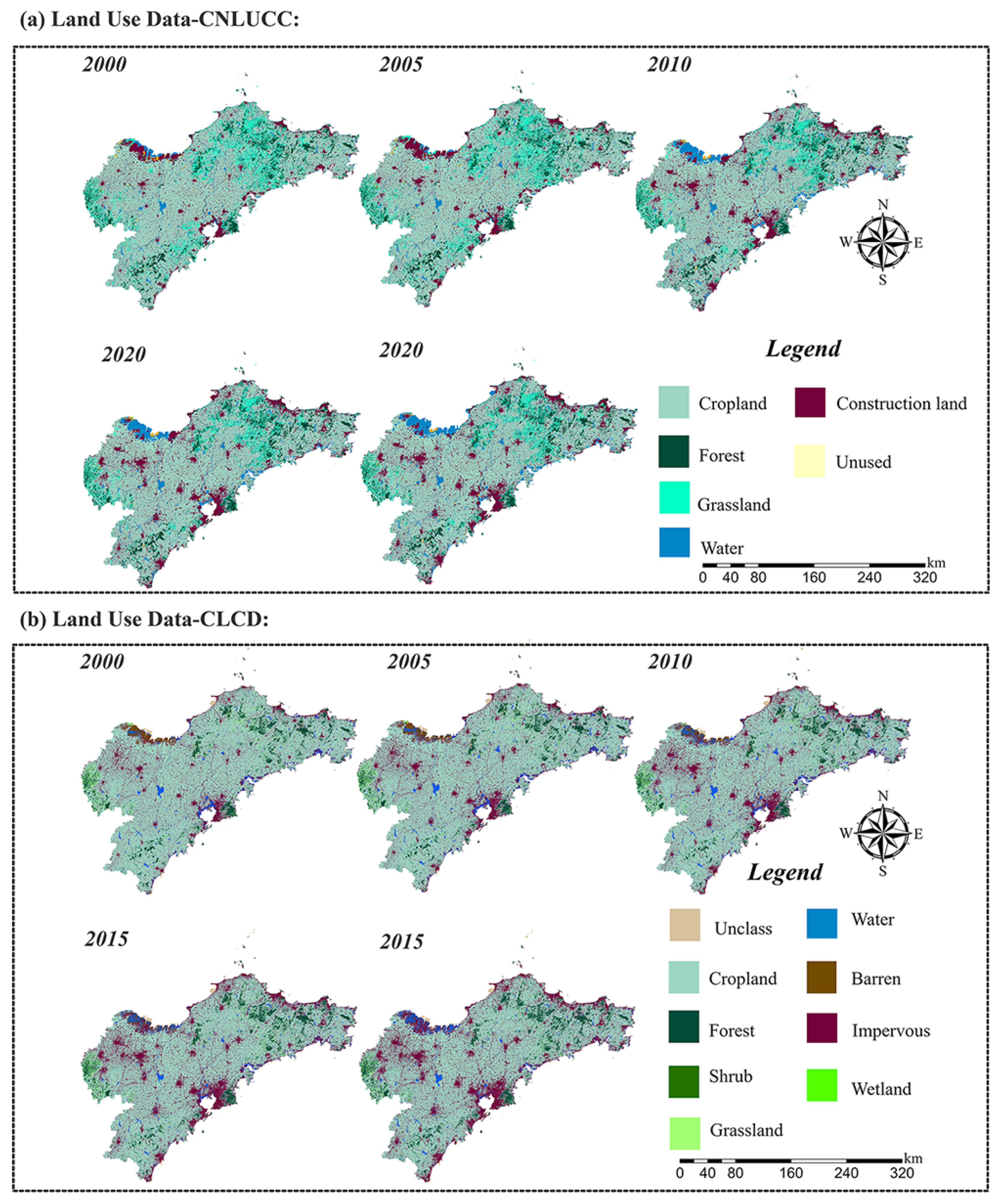
This study compared land use datasets and found mixed classifications of salt fields, seawater aquaculture areas, and coastal wetlands in the Jiaodong Peninsula. Coastal saline water and inland reservoirs were uniformly classified as water bodies (Figure A1). To better reflect LULC changes in coastal regions, we adopted a classification system for China’s coastal zones, distinguishing between inland water and saline water while merging shrubland and forest categories. As a result, the land use information for the Jiaodong Peninsula was reclassified (Table 2).
Table 2.
Land use hierarchy based on remote sensing techniques.
Landsat TM/ETM/OLI images were selected, processed for de-clouding, and mosaicked using the Google Earth Engine platform. Land types were visually calibrated with historical Google Earth images, setting 1406 sampling points. Land cover data for each period were generated using the Random Forest (RF) classification method. The dataset was split, with 70% for training the prediction model and 30% for validating accuracy. The classification accuracy was assessed using the Kappa coefficient as follows:
where represents the observed accuracy and represents the expected accuracy under random chance. In this study, was 92%, and the Kappa coefficient was 0.87, signifying reliable classification.
To further enhance representativeness and accuracy, the RF classification results were integrated with the CNLUCC and CLCD datasets using a non-homogeneous data voting approach. This method assesses consistency across multiple datasets via spatial overlay analysis based on a standardized classification system. For pixels with high consistency, the original classification was retained, while those with low consistency were refined using field survey data. Using this method, the classification accuracy improved to 94%, with a Kappa coefficient of 0.88. The final confusion matrix is shown in Table A1.
2.3.2. Climate Change Prediction
Description of Climate Scenarios
CMIP6 has been a key tool for global climate forecasting and modeling, providing precise climate models by integrating the RCP and SSP frameworks (ScenarioMIP Project). RCP scenarios, introduced in CMIP5, predict the impact of varying greenhouse gas concentrations on radiative forcing and global warming. The RCP framework includes RCP2.6, RCP4.5, RCP6.0, and RCP8.5, corresponding to global temperature increases of approximately 1.5 °C, 2.4 °C, 3–3.5 °C, and 4–5 °C by 2100, respectively. In CMIP6, the SSP1-5 framework describes how different social and economic development pathways influence emissions and land use. SSP1 represents a sustainable, low-emission society, while SSP5 envisions a high-emission, fossil-fuel-dependent economy.
Three representative scenarios, namely SSP1-2.6, SSP2-4.5, and SSP5-8.5, were selected to simulate climate changes on the Jiaodong Peninsula. SSP1-2.6 envisions sustainable development through the implementation of strict emission reduction policies, while SSP2-4.5 represents moderate climate action with gradual socio-economic progress. SSP5-8.5, a high-emission scenario, reflects rapid industrial growth with limited climate action, potentially leading to severe climate impacts.
Potential Evapotranspiration (PET) Inversion
Due to the absence of PET data output from the CMIP6 climate models, the Thornthwaite method was applied to calculate PET. The formula is outlined in Appendix A.2.
Bias Correction Method
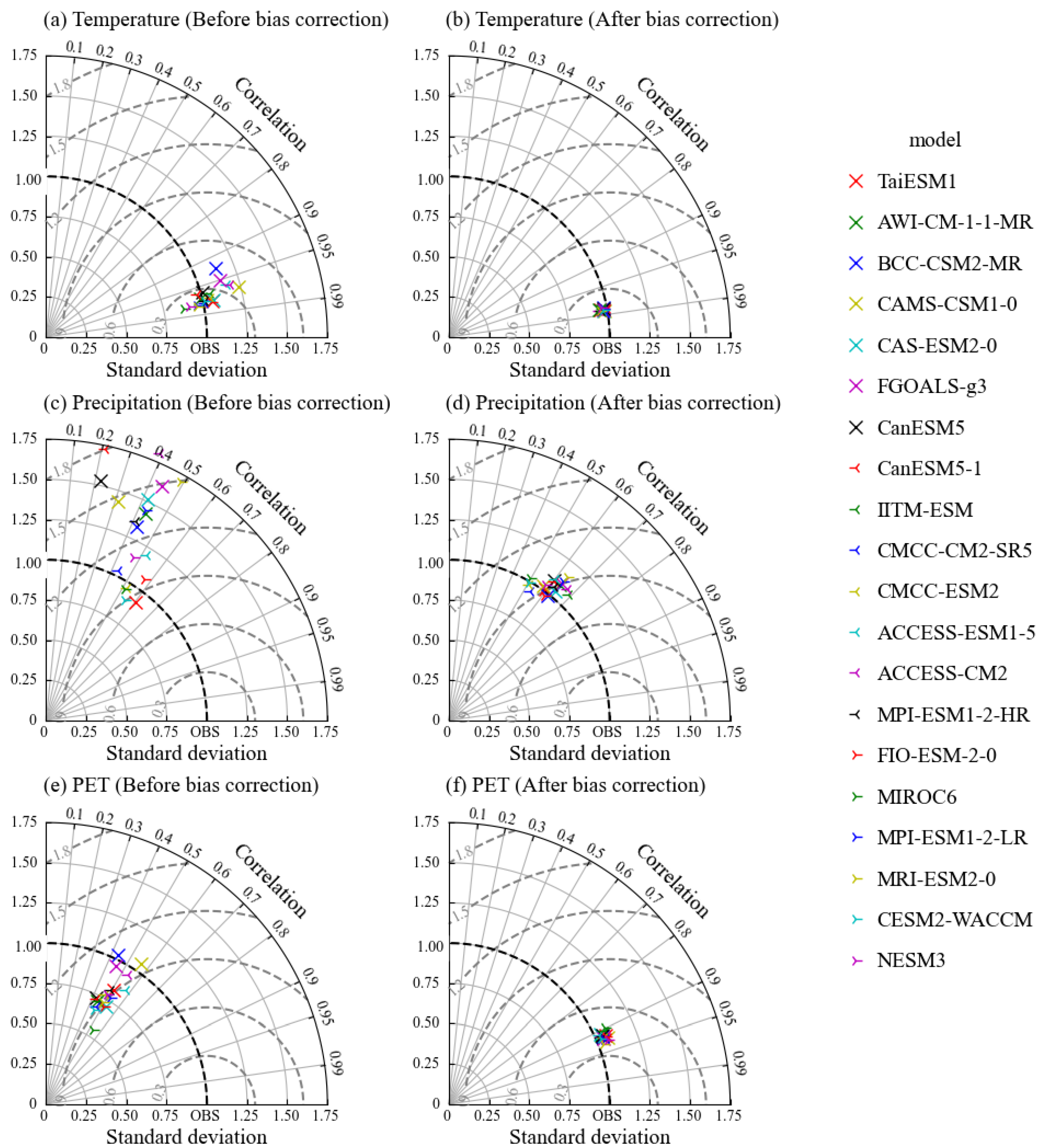
We selected 20 Atmosphere–Ocean Coupled Models (AOGCMs) from the CMIP6 dataset (Figure 3). Given that AOGCMs are global climate models with relatively coarse resolution and, thus, unable to capture small-scale spatial heterogeneity, bias correction is necessary when simulating local climate baselines. Referring to studies in the same region [35,36], the delta downscaling method was used for bias correction. The calculation formulas are expressed as follows:
where represents the corrected variable at grid i for month m and time t, is the value predicted by the model for the corresponding time and grid, represents the multi-year average observed value for the reference period at grid i for month m, and is the multi-year average value predicted by the model for the reference period at grid i for month m.
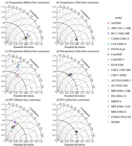
Figure 3.
Taylor diagram: (a,c,e) raw models’ outputs of monthly average temperature, monthly precipitation, and monthly PET; (b,d,f) outputs after delta downscaling; the radial lines represent the correlation coefficient, the horizontal and vertical axes indicate the standard deviation, and the dashed lines denote the root mean square error.
The reference period for this study is from 2009 to 2014. Temperature and precipitation grid observational data were derived from automatic weather station data using kriging interpolation, while PET data were sourced from ERA5-Land data.
Taylor diagrams comprehensively evaluate the performance of bias correction results [37,38]. By comparing the models’ simulation accuracy before and after delta downscaling with observation data from nine national stations in the Jiaodong Peninsula from 2000 to 2015 (with PET data interpolated from ERA5-Land data), it is evident that downscaling significantly improves the models’ predictive accuracy (Figure 3).
2.3.3. LULC Simulation under SSP-RCP Scenarios
The PLUS model has demonstrated high accuracy in simulating land use changes across diverse future scenarios [39,40]. By integrating CMIP6 SSP-RCP scenarios, it effectively forecasts LULC changes, particularly in complex coastal regions such as the Jiaodong Peninsula. The model consists of the following two core modules: the Land Expansion and Analysis Strategy (LEAS), which identifies LULC change regions and assesses their development potential, and Cellular Automata based on Multiple Random Seeds (CARS), which predicts LULC transitions by incorporating neighborhood effects and transition probabilities [41,42].
Estimation of RF-based Development Potential
After identifying and extracting the areas where LULC changes have occurred between two periods, the LEAS module converts these land use changes into a binary classification task. By applying the random forest (RF) classification algorithm, the PLUS model assesses the relationship between land use type growth and multiple influencing factors.
We selected 12 influencing factors from a diverse range of categories (Figure A2), including natural factors (aspect, DEM, and slope), climatic factors (PET, temperature, and precipitation), socio-economic factors (GDP, population density, and road density), and accessibility-related factors (distance to rivers, distance to railways, and distance to main transportation). This comprehensive parameterization captures key drivers of land use transformation, thereby improving the predictive accuracy and robustness of the model simulations.
CA-Markov Model Prediction
In the CARS module, the cellular automata (CA) model is a core component, providing dynamic simulation capabilities across both time and space. This allows the model to capture intricate spatial dependencies between land use types, which is critical in regions with complex features like the coastal and hilly terrain of the Jiaodong Peninsula. The Markov model complements this by offering long-term forecasts of land use transitions, enhancing predictive accuracy. Collectively, the CA-Markov model reduces simulation errors and improves LULC predictions for the region.
Optimizing the land transition matrices and neighborhood weights in the CARS module involves iterative trial-and-error adjustments (detailed in Table A2). This process integrates historical land use change data, climate scenario projections, anticipated socio-economic developments, and model validation results to refine key parameters incrementally. Through these iterations, the model improves its accuracy, making it more reliable and adaptable for long-term land use forecasts, especially in areas with complex geographical and climatic conditions.
Scenario Settings
CMIP6 SSP-RCP scenarios have been effectively applied in land use simulations, as they combine climate projections with socio-economic factors, enabling precise predictions of land use changes under varying policy and development conditions. We estimated the land use demands in 2030 and 2050 with the Markov model. Based on the future socio-economic development expectations under the three CMIP6 climate scenarios and referencing relevant studies [32,43], we established three future land use scenarios through the use of quantity constraints (Table 3).
Table 3.
Settings of scenarios in the PLUS model.
Model Validation and Accuracy
The PLUS model’s accuracy must be validated by testing its ability to replicate real data. We applied the built-in Kappa coefficient of the PLUS model to evaluate its suitability. Using land expansion samples and driving factor data from 2010–2015, the predicted results were compared with the actual LULC of 2020. This comparison allowed for the assessment of accuracy, and the optimal parameter settings were determined accordingly. The final model prediction achieved a Kappa coefficient of 0.85 and a value of 93%, reflecting reliable results that meet research requirements [44].
2.3.4. Assessment of Key ESs
Stanford University’s InVEST model is a widely applied tool for ES simulation [45]. By integrating climate simulation data from CMIP6 and land use prediction results from PLUS, the InVEST model can forecast future key ESs under SSP-RCP scenarios [31,32,33]. The WY module can reflect the water storage capacity of different landscapes [46]. The CS module calculates the total carbon stored in the landscape based on LULC data [4]. The SR module estimates the difference between potential soil loss, calculated using the Universal Soil Loss Equation (USLE) without vegetation cover, and actual soil loss (RKLS) with vegetation, as described by Ureta et al., (2020) [47]. The HQ module assesses the condition and quality of habitats with respect to biodiversity by evaluating the suitability of different habitat patches for wildlife and the intensity of threats surrounding those patches. According to the (InVEST User Guide (Project, 2024) (https://storage.googleapis.com/releases.naturalcapitalproject.org/invest-userguide/latest/en/index.html (accessed on 12 March 2024)) and related studies [34], we consider non-built-up areas as habitats, while built-up areas, cropland, saltwater, roads, railways, and other human-modified landscapes are regarded as threat sources. The calculation methods of WY, CS, SR, and HQ and the references for specific parameters can be found in Appendix A.4.
2.3.5. Analysis of Drivers of Future ESs
Structural equation modeling (SEM) is an analytical approach used to explore the connections between variables by assessing their covariance structure [48]. SEM allows for the assessment of the influence of individual indicators on the entire system, as well as the interconnections between these indicators. Unlike traditional analysis methods, SEM not only explores the covariance relationships but also accounts for the maximum variance among variables within the model, providing a more comprehensive understanding of the underlying relationships.
In ecological assessments, SEM allows for the use of multidimensional latent variables to construct a theoretical path relationship framework with a multi-level structure [49]. By modifying and adjusting the model based on quantitative indicators of overall goodness of fit, the reliability and stability of the model can be effectively enhanced. These characteristics of SEM contribute to the identification of the impacts of latent variables on complex ecosystems [50].The analysis was conducted using Python 3.11, with the fit indices of the SEM models provided in Table A6.
To find the driving mechanisms of the effects of future climate change and human activities on WY, CS, SR, and HQ, we constructed an SEM model using representative climate and human activity indicators informed by the ecological conditions of the Jiaodong Peninsula and previous research on its stress factors. The selected variables include annual average temperature (TEM), annual precipitation (PRE), annual PET, and the rainfall–runoff erosivity factor (PRR), corresponding to the input data R in the SR module of InVEST (Appendix A.4). The forest index (FI) reflects the proportion of forested area, while the urbanization index (BI) indicates the proportion of built-up area. Additional variables include population density (POP), elevation (DEM), and slope (Slope). These variables were utilized to construct the final SEM for the four key ecosystem services.
3. Results
3.1. Climate Changes from 2000 to 2050
The ensemble mean forecast results of 20 models are displayed in Figure 4. As indicated by the shaded areas, the differences between models increase over time, increasing the uncertainty of the model results. By 2050, the temperature, precipitation, and PET exhibit a significant upward trend, although the magnitude of change varies across all scenarios.
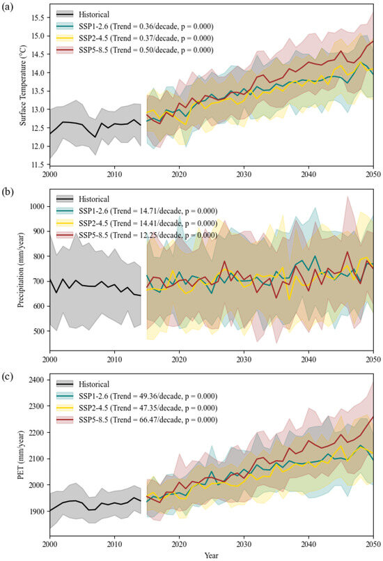
Figure 4.
Climate change projections: (a) Mean surface temperature, (b) Precipitation, (c) PET, with ensemble mean represented by solid lines and confidence intervals by shaded areas.
In the SSP1-2.6 scenario, the temperature shows the slowest increase trend, with a decadal increment of 0.36 °C. The precipitation increase is the largest, at 13.71 mm, and the PET increase is moderate, at 49.36 mm. The predicted values for 2050 under this scenario are 13.95 °C (temperature), 768.21 mm/year (precipitation), and 2094.41 mm/year (PET).
In the SSP2-4.5 scenario, which is comparable to SSP1-2.6, there is a larger increase in temperature. There are smaller increases in PET and precipitation. The predicted values for 2050 under this scenario are 14.10 °C (temperature), 752.14 mm/year (precipitation), and 2119.66 mm/year (PET).
The SSP5-8.5 scenario has the greatest increase trends in temperature and PET, with decadal increments of 0.50 °C and 66.47 mm, respectively. The precipitation increase is the smallest, at 12.25 mm. The predicted values for 2050 under this scenario are 14.85 °C (temperature), 749.33 mm/year (precipitation), and 2258.22 mm/year (PET).
3.2. The Spatiotemporal Changes of LULC from 2000 to 2050
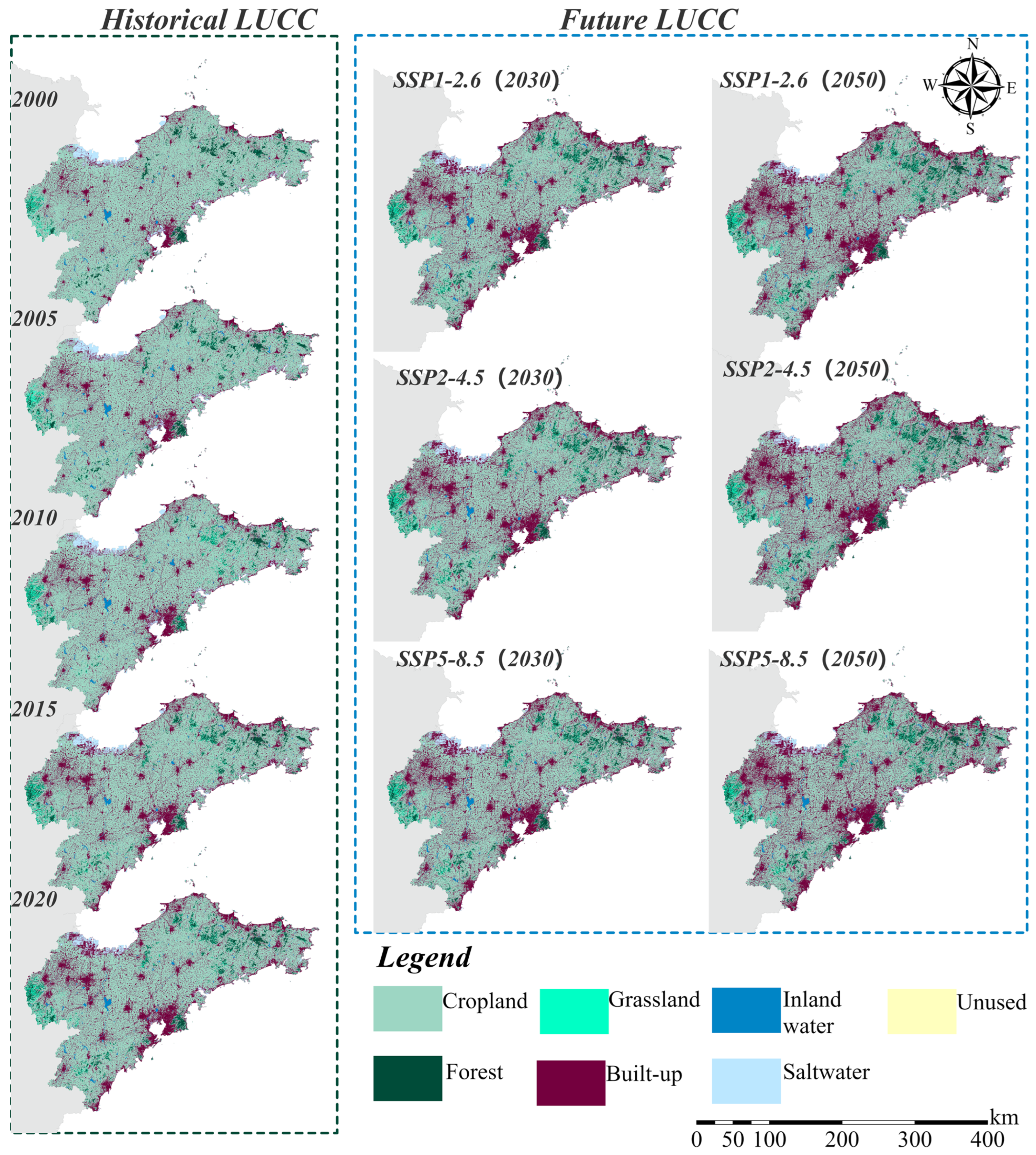
From 2000 to 2020, the main LULC types on the Jiaodong Peninsula were cropland and built-up land (Table 4). Cropland area declined from 77% in 2000 to 68% in 2020, whereas built-up area expanded from 15% to 25%. Due to the region’s rich coastal resources and significant trade ports like Qingdao Port, built-up areas primarily expanded along the coast (Figure 5). Forest land, mainly in high-altitude mountainous and hilly areas, was the third largest land type. Forest area decreased slowly before 2010, then increased to 5% after 2010. Saltwater areas declined consistently, making them the fourth largest land type. Grassland showed an overall increasing trend. Inland water bodies exhibited significant interannual fluctuations, reaching their lowest point in 2015 due to extreme drought. Unused land accounted for less than 1%, mainly in coastal areas.
Table 4.
Areas of LULC from 2000 to 2050.
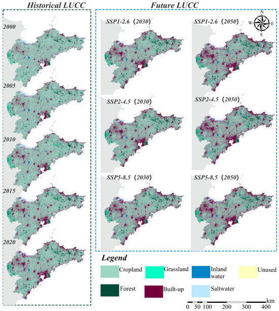
Figure 5.
Spatial distribution of LULC from 2000 to 2050.
From 2000 to 2020, the most major LULC change was the conversion of cropland to built-up area. This conversion peaked from 2010 to 2015 and was lowest from 2015 to 2020. The second most significant change from 2000 to 2010 was the conversion of forest land to cropland. From 2010 to 2015, the conversion of grassland to forest land was significant.There was a noticeable shift in coastal areas from seawater to developed land between 2015 and 2020.
Based on future climate trends and historical LULC trends, the PLUS model predicted future LULC changes under three scenarios (Figure 5). The spatial distribution of LULC in 2030 and 2050 generally mirrors the historical distribution. The main changes across all scenarios are characterized by a continued expansion of built-up areas and a corresponding decrease in cropland. Built-up areas are anticipated to grow particularly in historically dense and coastal regions. In the SSP5-8.5 scenario, built-up areas expand more than in the SSP2-4.5 and SSP1-2.6 scenarios.
In 2030 and 2050, forest and grassland areas are predicted to grow, mostly in mountainous and hilly regions, with the highest increase under SSP1-2.6. The proportion of inland water bodies remains stable around the 2020 level. Coastal saltwater areas generally decrease, except under SSP1-2.6 in 2030. Changes in unused land are not significant.
3.3. The Spatiotemporal Changes of Historical ESs
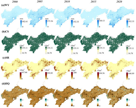
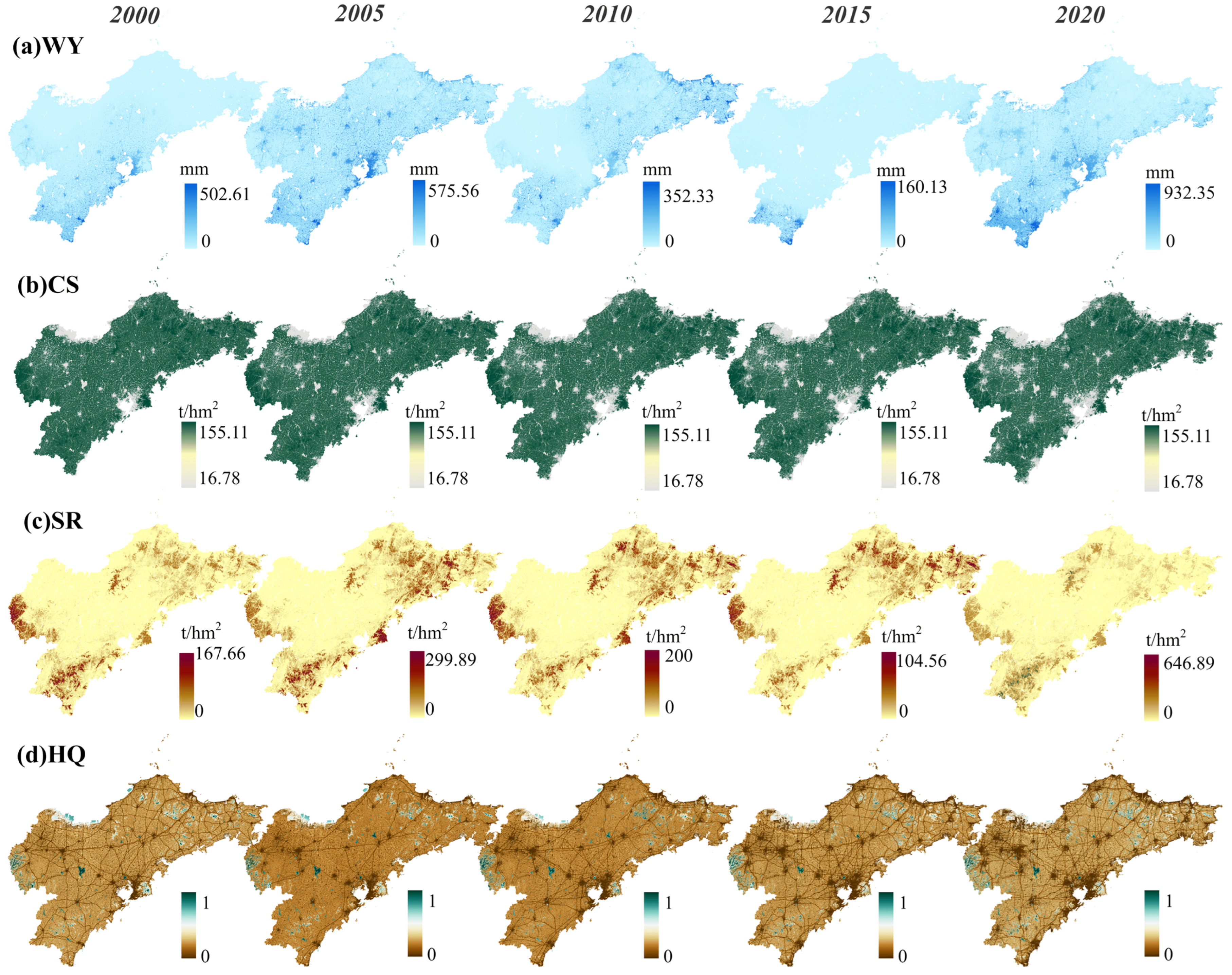
Figure 6.
Historical spatial distribution of key ESs from 2000 to 2020.
Table 5.
Changes of key ESs from 2000 to 2050.
- (1)
- Water yield (WY)The spatial distribution of WY is mainly influenced by LULC. High WY values are primarily concentrated in built-up areas, while low values are observed in inland water bodies, coastal saltwater areas, and forests. The interannual variation in WY is consistent with changes in precipitation, with the highest WY observed in 2020.
- (2)
- Carbon storage (CS)High CS is concentrated in mountainous and hilly areas, where forests and grasslands act as major carbon sinks. Inland water bodies exhibit the lowest carbon sequestration. CS shows a gradual decline, with an annual variation rate of −0.32 t/hm2. By 2020, CS had decreased by 6.69%.
- (3)
- Soil retention (SR)High SR is primarily located in mountainous and hilly areas. The steep terrain in these regions increases the susceptibility of soil to erosion. However, these areas are typically covered by woods and grasslands, which offer effective vegetation cover that intercepts and retains soil, thereby contributing to high SR. The interannual variation in soil retention is similar to that of WY and is consistent with changes in precipitation.
- (4)
- Habitat quality (HQ)High HQ is mainly located in hilly and mountainous places due to the existence of vast woods and grasslands, which provide suitable habitats for various species. Low HQ is found in inland built-up areas, transportation regions, and coastal saltwater zones. From 2000 to 2020, HQ on the Jiaodong Peninsula showed a declining trend, with an overall decrease of 9.13% by 2020.
3.4. Future ESs under SSP-RCP Scenarios
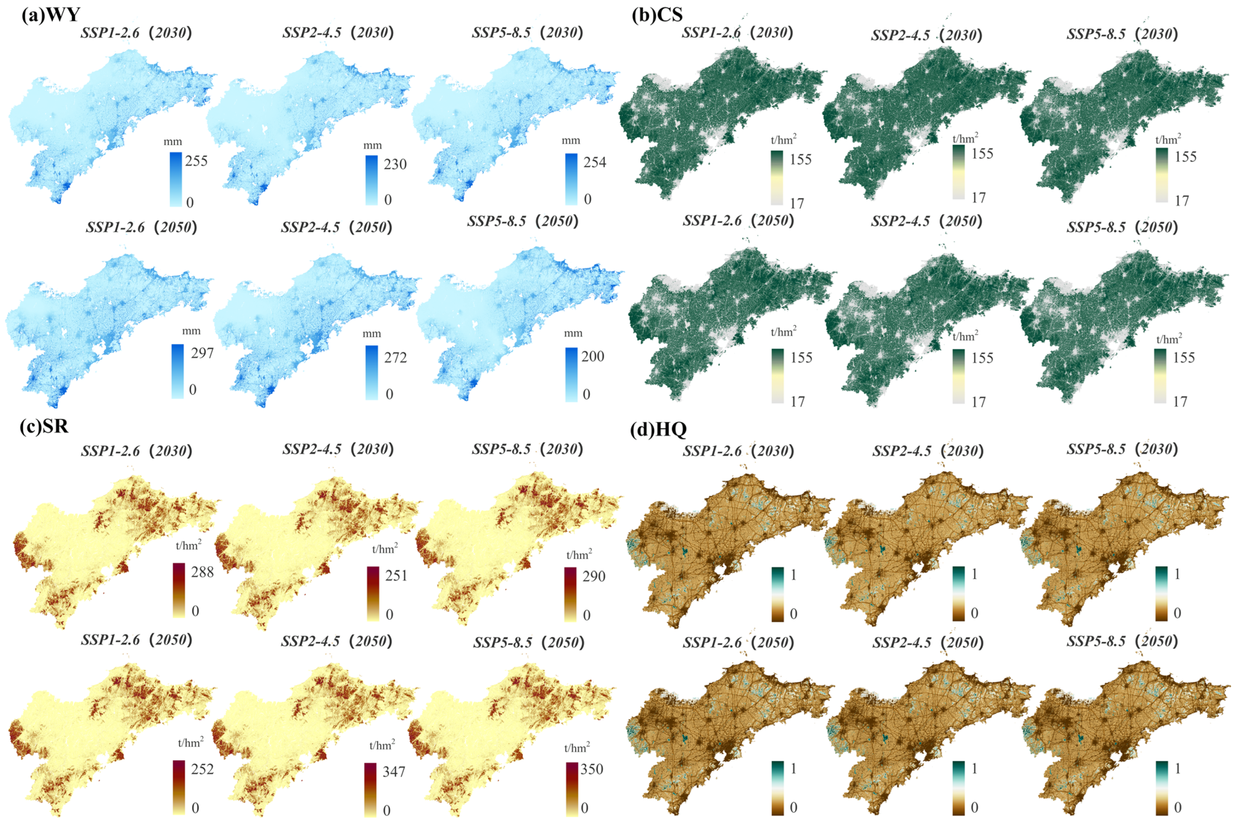
Figure 7 shows the future spatial distribution of WY, CS, SR, and HQ under SSP-RCP scenarios.
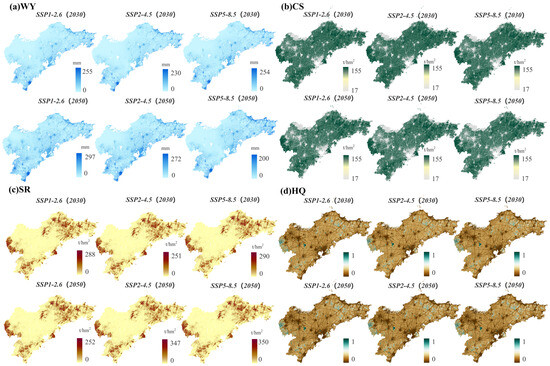
Figure 7.
Spatial Distribution of key ES under Different Scenarios.
- (1)
- WY under SSP-RCP ScenariosUnder the SSP1-2.6 and SSP2-4.5 scenarios, WY in 2050 is expected to be higher than in 2030 but lower than in 2020. The lowest WY in 2050 occurs under the SSP5-8.5 scenario, at only 56.79% of the SSP1-2.6 value. The spatial distribution of WY remains consistent with historical trends.
- (2)
- CS under SSP-RCP ScenariosFuture CS shows a declining trend across all scenarios, and the differences in CS between scenarios are small. by 2050, CS capacity follows the following order: SSP1-2.6 > SSP2-4.5 > SSP5-8.5, with CS under the SSP5-8.5 scenario being 8.59% lower than in 2020. The spatial distribution of CS remains consistent with historical trends.
- (3)
- SR under SSP-RCP ScenariosIn future scenarios, SR shows a decrease compared to 2020 but an increase relative to the 2000–2020 average (9.1 t/hm2). By 2050, SR is highest under the SSP5-8.5 scenario. The spatial distribution of SR remains consistent with historical trends.
- (4)
- HQ under SSP-RCP ScenariosHQ is projected to show a continuous decline in 2030 and 2050 across all scenarios. The greatest decline in HQ by 2050 is under SSP5-8.5, with a decrease of 9.13% compared to 2020, posing a significant threat to local biodiversity. HQ’s spatial distribution follows historical patterns, with higher concentrations in hilly regions.
3.5. Analysis of Drivers of ESs under Future SSP-RCP Scenarios
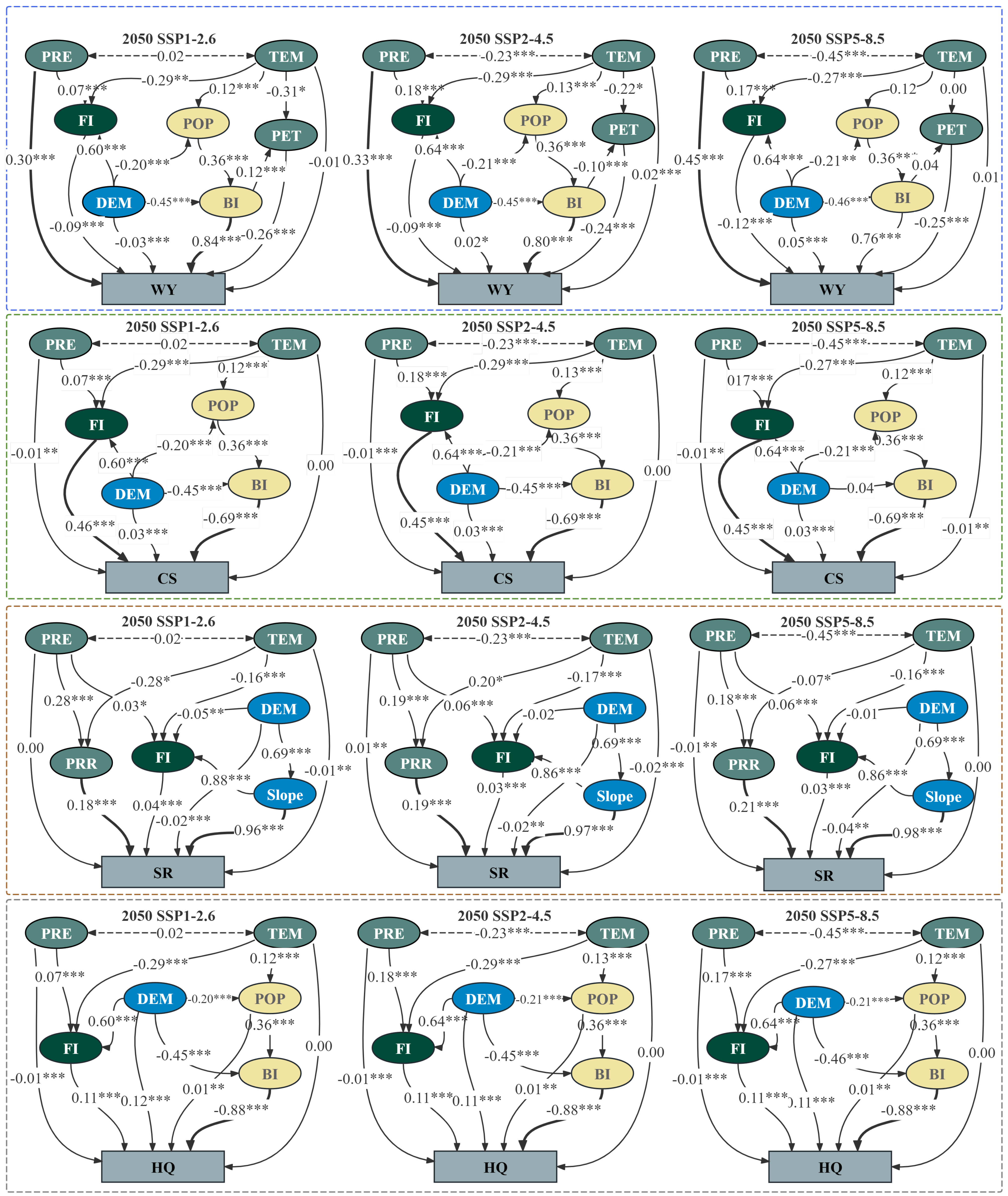
Figure 8 illustrates the effective application of SEM in identifying the key driving relationships for the four key ES in 2050. Detailed model metrics, including the comparative fit index (CFI), root mean square error of approximation (RMSEA), and AIC index, are provided in Table A6.
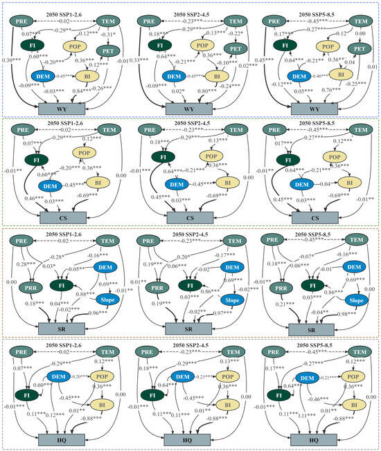
Figure 8.
SEM of factors influencing future WS, CS, SR, and HQ services ( * indicates significance at the 5% level; ** at the 1% level; *** at the 0.1% level).
3.5.1. Drivers of Future WY
Urbanization (BI) has a very strong positive correlation with WY, with path coefficients of 0.84, 0.80, and 0.76. This is due to the limited capacity of impermeable surfaces to retain precipitation, resulting in reduced available water content in these areas. Consequently, actual evapotranspiration (AET) is significantly lower than precipitation in these regions. In contrast, areas with high forest and vegetation cover (FI) capture precipitation and both surface and subsurface runoff through soil and vegetation. Due to continuous transpiration, these regions have experience higher levels of evapotranspiration than precipitation. The strong correlation between BI and WY suggests that human activities shape the spatial distribution of WY by altering land use patterns. PRE shows a strong positive correlation with WY, with path coefficients of 0.30, 0.33, and 0.45 across the three scenarios. The consistency between the interannual variations in WY and precipitation reflects this relationship. In contrast, PET is negatively correlated with WY, although the path coefficients is weaker than that of PRE. TEM has a limited direct impact on WY, but it can indirectly affect WY by influencing PET.
The correlation between BI and WY weakens across the three scenarios, while the correlation between PRE and WY strengthens. Additionally, PRE and TEM indirectly affect WY by influencing FI. This indicates that as climate change intensifies, climate factors may play a greater role in influencing WY functions.
3.5.2. Drivers of Future CS
CS is primarily influenced by BI and FI. Although forest areas increase to some extent in all three scenarios, the expansion of urban areas is much larger, leading to a declining trend in CS across all scenarios. The direct impact of climate on CS is minimal, and it only indirectly affects CS through FI. The differences in the correlation of various factors across the three scenarios are relatively small, indicating that human activities are the primary drivers impacting CS functionality.
3.5.3. Drivers of Future SR
Slope is the most significant factor influencing SR, with path coefficients exceeding 0.96 across all three scenarios. PPR is the most important meteorological factor affecting SR. The path coefficient of the effect of FI on SR is relatively small, primarily due to the strong collinearity between FI and slope, as forests in the Jiaodong Peninsula are mostly distributed in hilly and mountainous areas with steep slopes.
The influence of PPR on SR gradually increases across the three scenarios, with path coefficients of 0.18, 0.19, and 0.21. This indicates that as climate change intensifies, the impact of climatic factors on SR functions becomes more pronounced.
3.5.4. Drivers of Future HQ
In all three scenarios, BI is the decisive factor affecting HQ, showing a significant negative correlation, with a path coefficient of −0.88. PRE is negatively correlated with HQ, but the path coefficient is only −0.01, while HQ shows no correlation with TEM. PRE and TEM can only indirectly affect HQ through FI. The small differences in the path coefficients of various factors across the three scenarios indicate that the impact of climate change on HQ is minimal.
4. Discussion
4.1. Climate Changes and Future ES Protection
The SEM results (Figure 8) show a significant positive correlation between precipitation and both WY and SR, indicating that precipitation is the primary driver of the interannual variability and spatial distribution of WY and SR. Additionally, the spatial distribution of precipitation affects forest distribution, which indirectly influences CS and HQ functions. All scenarios predict an increase in precipitation (Figure 4), which directly and indirectly benefits these four key ecosystem functions. Compared to precipitation, the direct impact of annual mean temperature on key ESs is relatively minor, primarily affecting ESs indirectly by influencing FI. The increase in temperature across all scenarios is expected to hinder forest expansion, thereby weakening CS, SR, and HQ functions.
A horizontal comparison of the relationship between ESs and climate factors across the three scenarios reveals that the influence of PRE on WY and that of PRR on SR intensify with increasing human activity. Considering that all temperature and precipitation data used in this study are based on monthly averages, the differences in extreme climate events between the scenarios are not well captured. Using 2000–2010 as the baseline, the annual mean temperature on the Jiaodong Peninsula is projected to rise by 1.41 °C, 1.56 °C, and 2.31 °C by 2050 under the three scenarios (Figure 4). According to the Clausius–Clapeyron relationship, the probability of extreme precipitation events is expected to increase by 9.85%, 10.93%, and 16.18% [51,52], while rising temperatures will also lead to more extreme droughts [53,54]. These extreme climate events will enhance the erosive power of precipitation and increase surface PET. As a result, the impact of climate factors on WY and SR may be stronger than estimated in future scenarios.
Future climate change carries significant uncertainty, primarily stemming from the unpredictability of global greenhouse gas emissions, the complexity of natural climate systems, and region-specific responses to climate shifts [55]. In the Jiaodong Peninsula, climate models predict substantial changes in temperature and precipitation patterns, although the extent and precise impacts remain uncertain. Under this backdrop, the region’s ecosystem faces dual effects. On one hand, climate change may enhance ecosystem services, such as water supply and vegetation growth through increased precipitation; on the other hand, the heightened frequency and intensity of extreme events, like heavy rainfall and droughts, could pose serious threats to the ecosystem. Thus, the potential benefits and risks of climate change coexist, presenting considerable challenges for future ecosystem management in the Jiaodong Peninsula.
The government should prioritize strengthening water resource management in the region to address these challenges. Key measures include optimizing urban drainage systems to prevent flooding from extreme rainfall and enhancing agricultural irrigation infrastructure to mitigate the impact of droughts on crops and forest resources. Additionally, steep mountainous areas require improved forest protection to prevent soil erosion. Finally, meteorological agencies should enhance disaster prediction and early warning systems to help the public and authorities avoid risks and respond effectively to climate events. These actions are crucial for safeguarding the ecosystem and promoting sustainable social and economic development in the region.
4.2. Human Activities and Future ES Protection
Our study shows that human activities, particularly land use changes, and natural topography determine the spatial distribution of four key ESs in the Jiaodong Peninsula. As urbanization progresses, built-up areas continue to encroach on intensively cultivated cropland, leading to significant declines in CS and HQ. According to PLUS model simulations, under the SSP1-2.6 scenario, cropland will decrease by 8.5%, and CS and HQ will decline by 7% and 8.9%, respectively, by 2050. Under the SSP5-8.5 scenario, the cropland area will decrease by 9.2%, with further declines in CS and HQ of around 9% by 2050 (Table 4 and Table 5).
The northeastern and western regions of the Jiaodong Peninsula, characterized by high-altitude mountainous areas, are primarily covered by forest and grassland, providing high levels of CS, SR, and HQ (Figure 6 and Figure 7). By 2050, due to the government’s ongoing afforestation projects and the economic benefits of fruit cultivation, forest and grassland areas are expected to increase. However, even under SSP1-2.6, the total area of forest and grassland is projected to remain below 9%, which is insufficient to reverse the declines in CS and HQ (Table 4 and Table 5). In contrast, the coastal plains exhibit the lowest HQ values, with saltwater areas gradually being converted into unused and built-up areas, resulting in the loss of coastal habitats (Figure 6 and Figure 7). Overdevelopment has reduced natural coastal wetlands, affecting ecosystem stability and biodiversity [17]. Eutrophication from aquaculture has led to large-scale algal blooms [56], threatening marine species, and oil pollution from ships and ports has worsened coastal degradation [57]. PLUS simulations suggest that by 2050, suitable coastal habitats will shrink further, posing serious challenges for ecosystem protection.
Despite uncertainties in future socio-economic conditions and land use policies, our findings indicate that, without stricter land use restrictions, the degradation of key ESs will likely continue. However, extreme forest and grassland protection measures could negatively affect other ESs, such as WY. Limiting marine fisheries may also impact food supply services. Future studies should explore trade-offs and synergies between various ESs to achieve more sustainable management.
Balancing economic development and ecological protection remains a major challenge. We propose the following ecological protection measures: (1) Strictly limit urban expansion: Enforce stricter Cropland protection policies and increase green spaces in built-up areas to maintain habitat functions. (2) Optimize forest and grassland areas: Expand forest and grassland coverage to enhance CS and HQ and strengthen sand-fixation forests in mountainous areas to improve SR. (3) Strengthen coastal protection: Strictly limit development along natural coasts, control the scale of salt pans and aquaculture, establish eco-friendly marine farms, prevent nearshore pollution, restore natural beaches, protect wetlands, and enhance marine biodiversity.
4.3. Advantages and Limitations
To improve the accuracy of ES assessments and forecasts, we adopted a higher-resolution research scale. The examination and downscaling methods of the CMIP6 model outputs effectively corrected biases in future climate predictions. Additionally, we used random forest algorithms for land use classification of Landsat images, and the classification results were validated using data voting from multiple LULC datasets, significantly enhancing the accuracy of land use classification.
Our integrated research framework combines the CMIP6, PLUS, and InVEST models, providing a solid foundation for the assessment of future ESs under various climate and socio-economic scenarios. The SEM model was employed to analyze the internal driving mechanisms of ESs, revealing both direct and indirect effects of climate change and human activities while accounting for the interactions between these factors.
However, we acknowledge the uncertainties inherent in using complex models such as PLUS and InVEST. The results of the PLUS model are sensitive to assumptions and parameter settings regarding land use changes and socio-economic drivers, while the accuracy of the InVEST model depends heavily on the quality of input data such as climate and land use data. These uncertainties could introduce variability in ES projections. Although we attempted to mitigate some of these uncertainties by incorporating multiple LULC datasets and using downscaling techniques, a more comprehensive sensitivity analysis would better quantify the influence of different parameters on model outcomes. Future research should delve deeper into these uncertainties to improve the robustness of predictions.
There is still room for improvement in our study. As our research primarily focuses on assessing and predicting the impacts of future climate and land use changes on four key ESs and due to space limitations, we did not explore the potential synergies or trade-offs between these ESs in detail. Moreover, although we recognize that the impact of climate on ES may significantly increase under future scenarios, we lack in-depth research on the underlying mechanisms of these impacts.
5. Conclusions
We employed a CMIP6-PLUS-InVEST coupled prediction framework to explore the spatiotemporal changes of WY, CS, SR, and HQ under SSP-RCP scenarios from 2000 to 2050. Structural equation modeling (SEM) was used to reveal the complex effects of climate change and human activities on ESs.
The results indicate that the spatial distribution of ESs is primarily determined by human activities and natural topography, with WY being higher in built-up areas, while CS, SR, and HQ are mainly concentrated in mountainous regions. Under future scenarios, CS and HQ are projected to decline significantly due to urbanization, with the most severe declines observed under the SSP5-8.5 scenario. Precipitation is a key meteorological factor influencing WY and SR, with their interannual fluctuations aligning with precipitation levels. Temperature and precipitation also indirectly affect SR and HQ by influencing forest expansion. Compared to the SSP1-2.6 scenario, where human activity intensity is lower, the influence of climate factors on ES is stronger in the SSP5-8.5 scenario with higher human activity intensity. When considering the impact of temperature on extreme weather events, the effect of climate factors on ES is expected to further intensify under future warming scenarios.
This research offers a new perspective for future ES assessments under SSP-RCP scenarios. To address future ecosystem protection challenges and support sustainable development in the Jiaodong Peninsula, we provide several ecological and environmental management recommendations to policymakers with respect to climate change adaptation and human activity management. This study can be extended to other coastal regions.
Author Contributions
Conceptualization, W.G. and R.W.; methodology, W.G.; software, W.G.; validation, W.G. and R.W.; formal analysis, W.G.; investigation, W.G.; resources, W.G.; data curation, W.G. and F.M.; writing—original draft preparation, W.G. and F.M.; writing—review and editing, W.G. and R.W.; visualization, W.G.; supervision, R.W.; project administration, W.G.; funding acquisition, W.G. and F.M. All authors have read and agreed to the published version of the manuscript.
Funding
This research was supported by Research Projects of Qingdao Meteorological Bureau in 2023 (2023qdqxm03) and the Scientific Research Project of Shandong Meteorological Bureau in 2023 (2023SDBD12).
Institutional Review Board Statement
Not applicable.
Informed Consent Statement
Not applicable.
Data Availability Statement
The data presented in this study are available upon request from the corresponding author.
Conflicts of Interest
The authors declare no conflicts of interest.
Appendix A. Details of Materials and Methods
Appendix A.1. Data Preprocessing
Table A1.
Confusion matrix for land use reclassification.
Table A1.
Confusion matrix for land use reclassification.
| Visual Classification Results | Reclassification Results | ||||||
|---|---|---|---|---|---|---|---|
| Cropland | Forest | Grassland | Built-Up | Inland Water | Saltwater | Unused | |
| Cropland | 277 | 2 | 1 | 0 | 1 | 1 | 1 |
| Forest | 3 | 35 | 1 | 1 | 1 | 1 | 1 |
| Grassland | 1 | 1 | 12 | 1 | 0 | 0 | 0 |
| Built-up | 0 | 0 | 3 | 28 | 0 | 0 | 1 |
| Inland water | 1 | 0 | 0 | 0 | 16 | 1 | 0 |
| Saltwater | 1 | 0 | 0 | 0 | 2 | 19 | 0 |
| Unused | 1 | 0 | 0 | 0 | 0 | 0 | 8 |
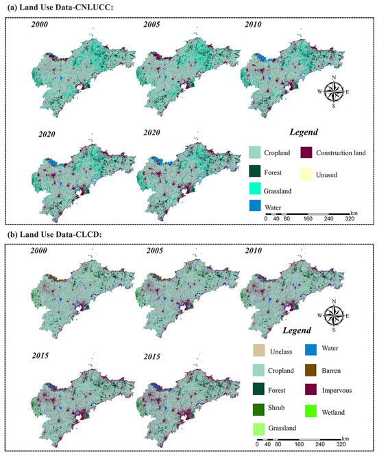
Figure A1.
Spatial distribution of LULC from the CNLUCC and CLCD datasets.
Figure A1.
Spatial distribution of LULC from the CNLUCC and CLCD datasets.
Appendix A.2. PET Inversion
The calculation formula of the Thornthwaite method is expressed as follows:
where is the PET for month i (mm/month), is the mean monthly temperature for month i (°C), and H is calculated using for the entire year. If is less than 0 °C, then is set to 0 and the PET for that month is 0 mm.
Appendix A.3. Inputs and Settings for the PLUS Model
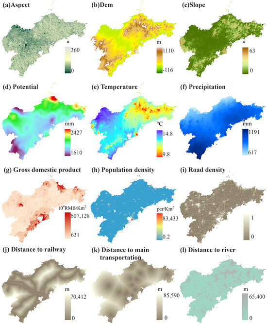
Figure A2.
Factors influencing LULC changes.
Figure A2.
Factors influencing LULC changes.

Table A2.
Neighborhood weights and land transition matrices.
Table A2.
Neighborhood weights and land transition matrices.
| Scenarios | Land Transition Matrices | Neighborhood Weight | |||||||
|---|---|---|---|---|---|---|---|---|---|
| Cropland | Forest | Grassland | Built-Up | Inland Water | Saltwater | Unused | |||
| SSP1-2.6 | Cropland | 1 | 1 | 1 | 1 | 0 | 1 | 0 | 0.9 |
| Forest | 1 | 1 | 1 | 1 | 0 | 1 | 0 | 0.16 | |
| Grassland | 1 | 1 | 1 | 1 | 0 | 1 | 0 | 0.07 | |
| Built-up | 1 | 1 | 1 | 1 | 0 | 1 | 0 | 0.76 | |
| Inland water | 0 | 0 | 0 | 0 | 1 | 0 | 0 | 0.2 | |
| Saltwater | 1 | 1 | 1 | 1 | 0 | 1 | 0 | 0.21 | |
| Unused | 0 | 0 | 0 | 0 | 0 | 0 | 1 | 0 | |
| SSP2-4.5 | Cropland | 1 | 1 | 1 | 1 | 0 | 1 | 1 | 0.9 |
| Forest | 1 | 1 | 1 | 1 | 0 | 1 | 1 | 0.16 | |
| Grassland | 1 | 1 | 1 | 1 | 0 | 1 | 1 | 0.07 | |
| Built-up | 1 | 1 | 1 | 1 | 0 | 1 | 1 | 0.76 | |
| Inland water | 0 | 0 | 0 | 0 | 1 | 0 | 1 | 0.2 | |
| Saltwater | 1 | 1 | 1 | 1 | 0 | 1 | 1 | 0.21 | |
| Unused | 1 | 1 | 1 | 1 | 1 | 1 | 1 | 0 | |
| SSP5-8.5 | Cropland | 1 | 1 | 1 | 0 | 0 | 0 | 0 | 0.9 |
| Forest | 1 | 1 | 1 | 1 | 0 | 0 | 0 | 0.16 | |
| Grassland | 1 | 1 | 1 | 1 | 0 | 0 | 0 | 0.07 | |
| Built-up | 1 | 1 | 1 | 1 | 0 | 0 | 0 | 0.76 | |
| Inland water | 0 | 0 | 0 | 0 | 1 | 0 | 0 | 0.2 | |
| Saltwater | 1 | 1 | 1 | 1 | 0 | 1 | 0 | 0.21 | |
| Unused | 1 | 1 | 1 | 1 | 1 | 1 | 1 | 0 | |
Appendix A.4. Inputs and Settings for the InVEST Model
Appendix A.4.1. Annual Water Yield (WY)
The annual water yield for grid x () is calculated as follows:
where is the actual annual evapotranspiration for grid x and is the annual precipitation.
The Budyko curve [58] is applied to calculate the for vegetated LULC types such as cropland, forest, and grassland, as follows:
For other LULCs,
where is the theoretical maximum evapotranspiration for grid x and is the Budyko parameter.
where is the PET for grid x and is the evapotranspiration coefficient associated with the LULC in grid x, which is set in Table A3. According to a study by Donohue [59], is defined as
where Z is set to and N is the number of rainy days in a year. is the volume of water content available for plants, which is defined as
The soil reference depth (), as used in this study, is derived from the China Soil Map-Based Harmonized World Soil Database (HWSD) [60]. The plant root depth () is specified according to relevant studies, with different root depths assigned for various land use types, as detailed in Table A3. The plant available water capacity () is calculated using the Hengl equation [61] as follows:
where – are seven available water capacity layers provided by SoilGrids 2017 data ranging in depth from 0 to 200 cm.
Appendix A.4.2. Carbon Storage (CS)
The carbon storage for a LULC type is calculated by summing four carbon pools, namely above-ground biomass (), below-ground biomass (), soil (), and dead organic matter (), as follows:
The CS module assumes that the carbon density of specific LULC types is constant. We synthesized multiple observational datasets from the study area [62] to obtain the carbon storage data for each LULC type (Table A3).
Appendix A.4.3. Soil Retention (SR)
In this study, ESs of erosion control provided by the landscape are quantified as avoided erosion () as follows:
The rainfall–runoff erosivity factor (R) is calculated using an empirical formula developed by Wischmeier [63] as follows:
where is the monthly precipitation for month i and is the annual precipitation.
The soil erodibility factor (K) is calculated by a corrected EPIC model formula [64,65] as follows:
where , , and represent the percentages of sand, silt, and clay content in the study area (%), respectively, and represents the percentage of organic carbon content (%), with all data provided by the China Soil Map-based HWSD dataset.
The slope-length gradient factor () is calculated based on DEM data using the 2D surface calculation method proposed by Desmet and Govers [66], which is an integral part of the InVEST model. For detailed calculation procedures, refer to the InVEST User Guide (Project, 2024) (https://storage.googleapis.com/releases.naturalcapitalproject.org/invest-userguide/latest/en/index.html (accessed on 12 March 2024)).
The values f the cover management factor (P) and support practice factor (C) are reported in Table A3.
Appendix A.4.4. Habitat Quality (HQ)
The habitat quality index for grid x in LULC j () is expressed as follows:
where is the habitat suitability of LULC type j; is habitat degradation; k is the half-saturation constant, typically set to 0.5; and z is fixed at 2.5 in the model by hard coding.
The value of habitat suitability () is reported in Table A5, and habitat degradation of LULC type j in grid x () is calculated as follows:
where is the number of grids of threat source r, is the weight of the threat, is the intensity of the threat source, and is the sensitivity of LULC type j to threat source r. is the impact of the threat source. Depending on the type of decay, the impact can be either linear or exponential. The calculation formulas are expressed as follows:
where represents the distance between grid x and grid y and denotes the maximum impact distance of threat source r in gird y.
Referencing the InVEST User Guide (Project, 2024) (https://storage.googleapis.com/releases.naturalcapitalproject.org/invest-userguide/latest/en/index.html (accessed on 1 March 2024)), and other related studies [34,67,68], the threat sources in this study were set as Built-up, cropland, saltwater, unused, road, and railway. Specific parameters are shown in Table A4 and Table A5.
Table A3.
InVEST parameter settings for LULC.
Table A3.
InVEST parameter settings for LULC.
| LULC Type | (mm) | (kg/hm2) | (kg/hm2) | (kg/hm2) | (kg/hm2) | P | C | |
|---|---|---|---|---|---|---|---|---|
| Cropland | 0.54 | 3500 | 7.74 | 5.26 | 95.4 | 1.32 | 0.22 | 0.4 |
| Forest | 0.83 | 5200 | 37.2 | 7.3 | 107.4 | 2.8 | 0.06 | 1 |
| Grassland | 0.54 | 2500 | 14.29 | 13.2 | 85.7 | 1.4 | 0.07 | 1 |
| Built-up | 0.25 | 100 | 1.81 | 1 | 14 | 0 | 0.2 | 0 |
| Inland water | 1.00 | 100 | 1.5 | 0.5 | 25.5 | 1.17 | 0 | 0 |
| Saltwater | 1.00 | 100 | 2 | 2.5 | 20 | 0.5 | 0 | 0 |
| Unused | 0.42 | 100 | 1.22 | 1.95 | 20.94 | 0.91 | 1 | 1 |
Table A4.
Threat source weight and maximum impact distances.
Table A4.
Threat source weight and maximum impact distances.
| Threat Source | Decay Type | ||
|---|---|---|---|
| Built-up | 1 | 9 | Exponential |
| Cropland | 0.4 | 3 | Linear |
| Saltwater | 0.1 | 1 | Linear |
| Unused | 0.8 | 1 | Exponential |
| Road | 0.6 | 0.5 | Linear |
| Railway | 0.6 | 0.5 | Linear |
Table A5.
Sensitivity of LULC.
Table A5.
Sensitivity of LULC.
| LULC Type | |||||||
|---|---|---|---|---|---|---|---|
| Built-Up | Cropland | Saltwater | Unused | Road | Railway | ||
| Cropland | 0.7 | 0.5 | 0 | 0.1 | 0.2 | 0.5 | 0.4 |
| Forest | 1 | 1 | 0.7 | 0 | 0.6 | 0.7 | 0.5 |
| Grassland | 1 | 0.7 | 0.6 | 0.1 | 0.4 | 0.4 | 0.3 |
| Built-up | 0 | 0 | 0 | 0 | 0 | 0 | 0 |
| Inland water | 0.9 | 0.6 | 0.4 | 0 | 0.2 | 0.4 | 0.2 |
| Saltwater | 0.8 | 0.6 | 0.4 | 0 | 0.3 | 0.3 | 0.2 |
| Unused | 0.1 | 0.6 | 0.2 | 0 | 0 | 0.3 | 0.1 |
Appendix A.5. Fit Indices of SEM Models
Table A6.
Fit indices of SEM models.
Table A6.
Fit indices of SEM models.
| Scenario | ES | CFI | GFI | AGFI | NFI | TLI | RMSEA | AIC | BIC |
|---|---|---|---|---|---|---|---|---|---|
| SSP1-2.6 | WY | 0.97 | 0.96 | 0.92 | 0.96 | 0.93 | 0.10 | 41.70 | 156.90 |
| CS | 0.98 | 0.97 | 0.95 | 0.97 | 0.95 | 0.11 | 33.74 | 126.99 | |
| SR | 0.92 | 0.92 | 0.80 | 0.92 | 0.81 | 0.22 | 35.03 | 133.77 | |
| HQ | 0.98 | 0.98 | 0.94 | 0.98 | 0.94 | 0.11 | 35.76 | 134.50 | |
| SSP2-4.5 | WY | 0.95 | 0.95 | 0.89 | 0.95 | 0.90 | 0.12 | 41.58 | 156.80 |
| CS | 0.98 | 0.97 | 0.94 | 0.97 | 0.95 | 0.11 | 33.72 | 127.00 | |
| SR | 0.92 | 0.92 | 0.80 | 0.92 | 0.80 | 0.22 | 35.02 | 133.78 | |
| HQ | 0.98 | 0.98 | 0.94 | 0.98 | 0.94 | 0.11 | 35.74 | 134.50 | |
| SSP5-8.5 | WY | 0.95 | 0.95 | 0.90 | 0.95 | 0.90 | 0.11 | 41.63 | 156.90 |
| CS | 0.98 | 0.97 | 0.94 | 0.97 | 0.95 | 0.11 | 33.72 | 127.03 | |
| SR | 0.90 | 0.90 | 0.75 | 0.90 | 0.75 | 0.25 | 34.71 | 133.51 | |
| HQ | 0.98 | 0.97 | 0.94 | 0.97 | 0.94 | 0.11 | 35.73 | 134.52 |
References
- Ross, S.R.J.; Arnoldi, J.F.; Loreau, M.; White, C.D.; Stout, J.C.; Jackson, A.L.; Donohue, I. Universal scaling of robustness of ecosystem services to species loss. Nat. Commun. 2021, 12, 5167. [Google Scholar] [CrossRef] [PubMed]
- Dobson, A.; Lodge, D.; Alder, J.; Cumming, G.S.; Keymer, J.; McGlade, J.; Mooney, H.; Rusak, J.A.; Sala, O.; Wolters, V.; et al. Habitat loss, trophic collapse, and the decline of ecosystem services. Ecology 2006, 87, 1915–1924. [Google Scholar] [CrossRef] [PubMed]
- McDowell, N.G.; Sapes, G.; Pivovaroff, A.; Adams, H.D.; Allen, C.D.; Anderegg, W.R.; Arend, M.; Breshears, D.D.; Brodribb, T.; Choat, B.; et al. Mechanisms of woody-plant mortality under rising drought, CO2 and vapour pressure deficit. Nat. Rev. Earth Environ. 2022, 3, 294–308. [Google Scholar] [CrossRef]
- Chen, X.; Yu, L.; Hou, S.; Liu, T.; Li, X.; Li, Y.; Du, Z.; Li, C.; Wu, H.; Gao, G.; et al. Unraveling carbon stock dynamics and their determinants in China’s Loess Plateau over the past 40 years. Ecol. Indic. 2024, 159, 111760. [Google Scholar] [CrossRef]
- Pecl, G.T.; Araújo, M.B.; Bell, J.D.; Blanchard, J.; Bonebrake, T.C.; Chen, I.C.; Clark, T.D.; Colwell, R.K.; Danielsen, F.; Evengård, B.; et al. Biodiversity redistribution under climate change: Impacts on ecosystems and human well-being. Science 2017, 355, eaai9214. [Google Scholar] [CrossRef]
- Fu, B.; Zhang, L.; Xu, Z.; Zhao, Y.; Wei, Y.; Skinner, D. Ecosystem services in changing land use. J. Soils Sediments 2015, 15, 833–843. [Google Scholar] [CrossRef]
- Yue, X.-L.; Gao, Q.-X. Contributions of natural systems and human activity to greenhouse gas emissions. Adv. Clim. Change Res. 2018, 9, 243–252. [Google Scholar] [CrossRef]
- Edo, G.I.; Itoje-akpokiniovo, L.O.; Obasohan, P.; Ikpekoro, V.O.; Samuel, P.O.; Jikah, A.N.; Nosu, L.C.; Ekokotu, H.A.; Ugbune, U.; Oghroro, E.E.A.; et al. Impact of environmental pollution from human activities on water, air quality and climate change. Ecol. Front. 2024, in press. [CrossRef]
- Yan, J.; Zhu, J.; Zhao, S.; Su, F. Coastal wetland degradation and ecosystem service value change in the Yellow River Delta, China. Glob. Ecol. Conserv. 2023, 44, e02501. [Google Scholar] [CrossRef]
- Watson, C.S.; Kargel, J.S.; Regmi, D.; Rupper, S.; Maurer, J.M.; Karki, A. Shrinkage of Nepal’s second largest lake (Phewa Tal) due to watershed degradation and increased sediment influx. Remote Sens. 2019, 11, 444. [Google Scholar] [CrossRef]
- Wu, X.; Wang, L.; Yao, R.; Luo, M.; Li, X. Identifying the dominant driving factors of heat waves in the North China Plain. Atmos. Res. 2021, 252, 105458. [Google Scholar] [CrossRef]
- Gampe, D.; Zscheischler, J.; Reichstein, M.; O’Sullivan, M.; Smith, W.K.; Sitch, S.; Buermann, W. Increasing impact of warm droughts on northern ecosystem productivity over recent decades. Nat. Clim. Change 2021, 11, 772–779. [Google Scholar] [CrossRef]
- Konapala, G.; Mishra, A.K.; Wada, Y.; Mann, M.E. Climate change will affect global water availability through compounding changes in seasonal precipitation and evaporation. Nat. Commun. 2020, 11, 3044. [Google Scholar] [CrossRef] [PubMed]
- Taboada, A.; García-Llamas, P.; Fernández-Guisuraga, J.M.; Calvo, L. Wildfires impact on ecosystem service delivery in fire-prone maritime pine-dominated forests. Ecosyst. Serv. 2021, 50, 101334. [Google Scholar] [CrossRef]
- Perkins, K.M.; Munguia, N.; Ellenbecker, M.; Moure-Eraso, R.; Velazquez, L. COVID-19 pandemic lessons to facilitate future engagement in the global climate crisis. J. Clean. Prod. 2021, 290, 125178. [Google Scholar] [CrossRef]
- Grima, N.; Corcoran, W.; Hill-James, C.; Langton, B.; Sommer, H.; Fisher, B. The importance of urban natural areas and urban ecosystem services during the COVID-19 pandemic. PLoS ONE 2020, 15, e0243344. [Google Scholar] [CrossRef]
- Dong, J.Y.; Guo, M.; Wang, X.; Yang, o.; Zhang, Y.H.; Zhang, P.D. Dramatic loss of seagrass Zostera marina L. suitable habitat under projected climate change in coastal areas of the Bohai Sea and Shandong peninsula, China. J. Exp. Mar. Biol. Ecol. 2023, 565, 151915. [Google Scholar] [CrossRef]
- Xu, X.; Qiao, S.; Jiang, H.; Zhang, T. Ecosystem vulnerability to extreme climate in coastal areas of China. Environ. Res. Lett. 2023, 18, 124028. [Google Scholar]
- Xia, J.; Yang, X.Y.; Liu, J.; Wang, M.; Li, J. Dominant change pattern of extreme precipitation and its potential causes in Shandong Province, China. Sci. Rep. 2022, 12, 858. [Google Scholar]
- Guo, W.; Wang, R. Spatiotemporal Evolution of Ecological Environment Quality and Driving Factors in Jiaodong Peninsula, China. Sustainability 2024, 16, 3676. [Google Scholar] [CrossRef]
- Yuan, Y.; Song, D.; Wu, W.; Liang, S.; Wang, Y.; Ren, Z. The impact of anthropogenic activities on marine environment in Jiaozhou Bay, Qingdao, China: A review and a case study. Reg. Stud. Mar. Sci. 2016, 8, 287–296. [Google Scholar] [CrossRef]
- Ai, B.; Tian, Y.; Wang, P.; Gan, Y.; Luo, F.; Shi, Q. Vulnerability analysis of coastal zone based on InVEST model in Jiaozhou Bay, China. Sustainability 2022, 14, 6913. [Google Scholar] [CrossRef]
- Mu, H.; Wang, Y.; Zhang, H.; Guo, F.; Li, A.; Zhang, S.; Liu, S.; Liu, T. High abundance of microplastics in groundwater in Jiaodong Peninsula, China. Sci. Total Environ. 2022, 839, 156318. [Google Scholar] [CrossRef] [PubMed]
- Liu, S.; Zhu, L.; Jiang, W.; Qin, J.; Lee, H.S. Research on the effects of soil petroleum pollution concentration on the diversity of natural plant communities along the coastline of Jiaozhou bay. Environ. Res. 2021, 197, 111127. [Google Scholar] [CrossRef] [PubMed]
- Zhao, L.; Yang, C.h.; Zhao, Y.c.; Wang, Q.; Zhang, Q.p. Spatial correlations of land use carbon emissions in Shandong peninsula urban agglomeration: A perspective from city level using remote sensing data. Remote Sens. 2023, 15, 1488. [Google Scholar] [CrossRef]
- Ouyang, K.; Huang, M.; Gong, D.; Zhu, D.; Lin, H.; Xiao, C.; Fan, Y.; Altan, O. A Novel Framework for Integrally Evaluating the Impacts of Climate Change and Human Activities on Water Yield Services from Both Local and Global Perspectives. Remote Sens. 2024, 16, 3008. [Google Scholar] [CrossRef]
- Qiao, X.; Li, Z.; Lin, J.; Wang, H.; Zheng, S.; Yang, S. Assessing current and future soil erosion under changing land use based on InVEST and FLUS models in the Yihe River Basin, North China. Int. Soil Water Conserv. Res. 2024, 12, 298–312. [Google Scholar] [CrossRef]
- He, Y.; Ma, J.; Zhang, C.; Yang, H. Spatio-temporal evolution and prediction of carbon storage in Guilin based on FLUS and InVEST models. Remote Sens. 2023, 15, 1445. [Google Scholar] [CrossRef]
- Tebaldi, C.; Debeire, K.; Eyring, V.; Fischer, E.; Fyfe, J.; Friedlingstein, P.; Knutti, R.; Lowe, J.; O’Neill, B.; Sanderson, B.; et al. Climate model projections from the scenario model intercomparison project (ScenarioMIP) of CMIP6. Earth Syst. Dyn. 2021, 12, 253–293. [Google Scholar] [CrossRef]
- You, Q.; Cai, Z.; Wu, F.; Jiang, Z.; Pepin, N.; Shen, S.S. Temperature dataset of CMIP6 models over China: Evaluation, trend and uncertainty. Clim. Dyn. 2021, 57, 17–35. [Google Scholar]
- Li, J.; Chen, X.; Kurban, A.; Van de Voorde, T.; De Maeyer, P.; Zhang, C. Coupled SSPs-RCPs scenarios to project the future dynamic variations of water-soil-carbon-biodiversity services in Central Asia. Ecol. Indic. 2021, 129, 107936. [Google Scholar] [CrossRef]
- Ji, X.; Sun, Y.; Guo, W.; Zhao, C.; Li, K. Land use and habitat quality change in the Yellow River Basin: A perspective with different CMIP6-based scenarios and multiple scales. J. Environ. Manag. 2023, 345, 118729. [Google Scholar] [CrossRef]
- Guo, W.; Teng, Y.; Li, J.; Yan, Y.; Zhao, C.; Li, Y.; Li, N. A new assessment framework to forecast land use and carbon storage under different SSP-RCP scenarios in China. Sci. Total Environ. 2024, 912, 169088. [Google Scholar] [CrossRef] [PubMed]
- Liao, J.; Zhang, D.; Su, S.; Liang, S.; Du, J.; Yu, W.; Ma, Z.; Chen, B.; Hu, W. Coastal habitat quality assessment and mapping in the terrestrial-marine continuum: Simulating effects of coastal management decisions. Ecol. Indic. 2023, 156, 111158. [Google Scholar] [CrossRef]
- Wilby, R.L.; Charles, S.P.; Zorita, E.; Timbal, B.; Whetton, P.; Mearns, L.O. Guidelines for Use of Climate Scenarios Developed from Statistical Downscaling Methods. Supporting Material of the Intergovernmental Panel on Climate Change, Available from the DDC of IPCC TGCIA. 2004, Volume 27. Available online: https://www.ipcc-data.org/guidelines/dgm_no2_v1_09_2004.pdf (accessed on 4 January 2020).
- Zhao, F.; Xu, Z. Comparative analysis on downscaled climate scenarios for headwater catchment of Yellow River using SDS and delta methods. Acta Meteorol. Sin. 2007, 65, 653–662. [Google Scholar]
- Yan, D.; Werners, S.E.; Ludwig, F.; Huang, H.Q. Hydrological response to climate change: The Pearl River, China under different RCP scenarios. J. Hydrol. Reg. Stud. 2015, 4, 228–245. [Google Scholar] [CrossRef]
- Rivera, J.A.; Arnould, G. Evaluation of the ability of CMIP6 models to simulate precipitation over Southwestern South America: Climatic features and long-term trends (1901–2014). Atmos. Res. 2020, 241, 104953. [Google Scholar] [CrossRef]
- Fang, Z.; Ding, T.; Chen, J.; Xue, S.; Zhou, Q.; Wang, Y.; Wang, Y.; Huang, Z.; Yang, S. Impacts of land use/land cover changes on ecosystem services in ecologically fragile regions. Sci. Total Environ. 2022, 831, 154967. [Google Scholar] [CrossRef] [PubMed]
- Yi, F.; Yang, Q.; Wang, Z.; Li, Y.; Cheng, L.; Yao, B.; Lu, Q. Changes in land use and ecosystem service values of Dunhuang Oasis from 1990 to 2030. Remote Sens. 2023, 15, 564. [Google Scholar] [CrossRef]
- Liu, X.; Liang, X.; Li, X.; Xu, o.; Ou, J.; Chen, Y.; Li, S.; Wang, S.; Pei, F. A future land use simulation model (FLUS) for simulating multiple land use scenarios by coupling human and natural effects. Landsc. Urban Plan. 2017, 168, 94–116. [Google Scholar] [CrossRef]
- Liang, X.; Liu, o.; Li, D.; Zhao, H.; Chen, G. Urban growth simulation by incorporating planning policies into a CA-based future land-use simulation model. Int. J. Geogr. Inf. Sci. 2018, 32, 2294–2316. [Google Scholar] [CrossRef]
- Liu, Q.; Yang, D.; Cao, L.; Anderson, B. Assessment and prediction of carbon storage based on land use/land cover dynamics in the tropics: A case study of hainan island, China. Land 2022, 11, 244. [Google Scholar] [CrossRef]
- Liang, Y.; Liu, L.; Huang, J. Integrating the SD-CLUE-S and InVEST models into assessment of oasis carbon storage in northwestern China. PLoS ONE 2017, 12, e0172494. [Google Scholar] [CrossRef] [PubMed]
- Ai, X.; Zheng, X.; Zhang, Y.; Liu, Y.; Ou, X.; Xia, C.; Liu, L. Climate and land use changes impact the trajectories of ecosystem service bundles in an urban agglomeration: Intricate interaction trends and driver identification under SSP-RCP scenarios. Sci. Total Environ. 2024, 944, 173828. [Google Scholar] [CrossRef] [PubMed]
- Li, Y.; Liu, W.; Feng, Q.; Zhu, M.; Yang, L.; Zhang, J.; Yin, X. The role of land use change in affecting ecosystem services and the ecological security pattern of the Hexi Regions, Northwest China. Sci. Total Environ. 2023, 855, 158940. [Google Scholar] [CrossRef]
- Ureta, J.C.; Clay, L.; Motallebi, M.; Ureta, J. Quantifying the landscape’s ecological benefits—An analysis of the effect of land cover change on ecosystem services. Land 2020, 10, 21. [Google Scholar] [CrossRef]
- Hair, J.F., Jr.; Hult, G.T.M.; Ringle, C.M.; Sarstedt, M.; Danks, N.P.; Ray, S. Partial least squares structural equation modeling (PLS-SEM) using R: A workbook; Springer: Berlin/Heidelberg, Germany, 2021; pp. 1–29. [Google Scholar]
- Fan, Y.; Chen, J.; Shirkey, G.; John, R.; Wu, S.R.; Park, H.; Shao, C. Applications of structural equation modeling (SEM) in ecological studies: An updated review. Ecol. Process. 2016, 5, 19. [Google Scholar] [CrossRef]
- Qiu, J.; Yu, D.; Huang, T. Influential paths of ecosystem services on human well-being in the context of the sustainable development goals. Sci. Total Environ. 2022, 852, 158443. [Google Scholar] [CrossRef] [PubMed]
- Koutsoyiannis, D. Clausius–Clapeyron equation and saturation vapour pressure: Simple theory reconciled with practice. Eur. J. Phys. 2012, 33, 295. [Google Scholar] [CrossRef]
- Neelin, J.D.; Martinez-Villalobos, C.; Stechmann, S.N.; Ahmed, F.; Chen, G.; Norris, J.M.; Kuo, Y.H.; Lenderink, G. Precipitation extremes and water vapor: Relationships in current climate and implications for climate change. Curr. Clim. Change Rep. 2022, 8, 17–33. [Google Scholar] [CrossRef]
- Masson-Delmotte, V.; Zhai, P.; Pörtner, H.O.; Roberts, D.; Skea, J.; Shukla, P.R. Global Warming of 1.5 C: IPCC Special Report on Impacts of Global Warming of 1.5 C above Pre-Industrial Levels in Context of Strengthening Response to Climate Change, Sustainable Development, and Efforts to Eradicate Poverty; Cambridge University Press: Cambridge, UK, 2022. [Google Scholar]
- Li, Z.; Fang, G.; Chen, Y.; Duan, W.; Mukanov, Y. Agricultural water demands in Central Asia under 1.5 C and 2.0 C global warming. Agric. Water Manag. 2020, 231, 106020. [Google Scholar] [CrossRef]
- Seidenfaden, I.K.; Jensen, K.H.; Sonnenborg, T.O. Climate change impacts and uncertainty on spatiotemporal variations of drought indices for an irrigated catchment. J. Hydrol. 2021, 601, 126814. [Google Scholar]
- Xu, Y.; Xu, T. An evolving marine environment and its driving forces of algal blooms in the Southern Yellow Sea of China. Mar. Environ. Res. 2022, 178, 105635. [Google Scholar] [CrossRef]
- Wang, Y.; Du, P.; Liu, B.; Sheng, S. Vulnerability of mariculture areas to oil-spill stress in waters north of the Shandong Peninsula, China. Ecol. Indic. 2023, 148, 110107. [Google Scholar] [CrossRef]
- Budyko, M.I.; Miller, D.H. Climate and Life; Academic Press: New York, NY, USA, 1974; p. 508. [Google Scholar]
- Donohue, R.J.; Roderick, M.L.; McVicar, T.R. Roots, storms and soil pores: Incorporating key ecohydrological processes into Budyko’s hydrological model. J. Hydrol. 2012, 436, 35–50. [Google Scholar] [CrossRef]
- Fischer, G.; Nachtergaele, F.; Prieler, S.; Van Velthuizen, H.; Verelst, L.; Wiberg, D. Global Agro-Ecological Zones Assessment for Agriculture (GAEZ 2008); IIASA: Laxenburg, Austria; FAO: Rome, Italy, 2008; Volume 10. [Google Scholar]
- Hengl, T.; Mendes de Jesus, J.; Heuvelink, G.B.; Ruiperez Gonzalez, M.; Kilibarda, M.; Blagotić, A.; Shangguan, W.; Wright, M.N.; Geng, O.; Bauer-Marschallinger, B.; et al. SoilGrids250m: Global gridded soil information based on machine learning. PLoS ONE 2017, 12, e0169748. [Google Scholar] [CrossRef]
- Xu, L.; He, N.; Yu, G. A dataset of carbon density in Chinese terrestrial ecosystems (2010s). China Sci. Data 2019, 4, 90–96. [Google Scholar]
- Wischmeier, W.H.; Smith, D.D. Predicting Rainfall Erosion Losses: A Guide to Conservation Planning; Number 537, Department of Agriculture, Science and Education Administration. 1978. Available online: https://www.ars.usda.gov/ARSUserFiles/60600505/RUSLE/AH_537%20Predicting%20Rainfall%20Soil%20Losses.pdf (accessed on 1 August 2024).
- Williams, J.; Renard, K.; Dyke, P. EPIC: A new method for assessing erosion’s effect on soil productivity. J. Soil Water Conserv. 1983, 38, 381–383. [Google Scholar]
- Zhang, K.; Peng, W.; Yang, H. Soil erodibility values and their estimation in China. Acta Pedofil. Sin 2007, 44, 7–13. [Google Scholar]
- Desmet, P.J.; Govers, G. A GIS procedure for automatically calculating the USLE LS factor on topographically complex landscape units. J. Soil Water Conserv. 1996, 51, 427–433. [Google Scholar]
- Yang, Y. Evolution of habitat quality and association with land-use changes in mountainous areas: A case study of the Taihang Mountains in Hebei Province, China. Ecol. Indic. 2021, 129, 107967. [Google Scholar] [CrossRef]
- Feng, Z.; Jin, X.; Chen, T.; Wu, J. Understanding trade-offs and synergies of ecosystem services to support the decision-making in the Beijing–Tianjin–Hebei region. Land Use Policy 2021, 106, 105446. [Google Scholar] [CrossRef]

Disclaimer/Publisher’s Note: The statements, opinions and data contained in all publications are solely those of the individual author(s) and contributor(s) and not of MDPI and/or the editor(s). MDPI and/or the editor(s) disclaim responsibility for any injury to people or property resulting from any ideas, methods, instructions or products referred to in the content. |
© 2024 by the authors. Licensee MDPI, Basel, Switzerland. This article is an open access article distributed under the terms and conditions of the Creative Commons Attribution (CC BY) license (https://creativecommons.org/licenses/by/4.0/).