Abstract
A fast and accurate radiative transfer model is the prerequisite in the field of atmospheric remote sensing for limb atmospheric inversion to tackle the drawback of slow calculation speed of traditional atmospheric radiative transfer models. This paper established a fast computing model (ANN-HASFCM) for high-spectral-resolution absorption spectra by using artificial neural networks and PCA (principal component analysis) spectral reconstruction technology. This paper chose the line-by-line radiative transfer model (LBLRTM) as the comparative model and simulated training spectral data in the oxygen A-band (12,900–13,200 cm−1). Subsequently, ANN-HASFCM was applied to the retrieval of the atmospheric density profile with the data of the Global Ozone Monitoring by an Occultation of Stars (GOMOS) instrument. The results show that the relative error between the optical depth spectra calculated by LBLRTM and ANN-HASFCM is within 0.03–0.65%. In the process of using the global-fitting algorithm to invert GOMOS-measured atmospheric samples, the inversion results using Fast-LBLRTM and ANN-HASFCM as forward models are consistent, and the retrieval speed of ANN-HASFCM is more than 200 times faster than that of Fast-LBLRTM (reduced from 226.7 s to 0.834 s). The analysis shows the brilliant application prospects of ANN-HASFCM in limb remote sensing.
1. Introduction
Oxygen is evenly distributed in the atmosphere with a constant mixing ratio, and in the A absorption band, there is basically no interference of other gas absorption, which belongs to a relatively pure absorption band. In addition, the oxygen A-band is an ideal inversion channel with advantages such as strong spectral line intensity and a wide dynamic range of transmittance. Limb occultation observation, as an atmospheric observation mode where the line of sight passes over the earth’s surface at a certain tangential height while the space detector is aimed at the star, has advantages such as superior coverage, high vertical resolution and no need for calibration. Consequently, a growing number of atmospheric scientists are paying attention to the method of using oxygen A-band to inverse limb atmospheric parameters [1,2,3,4,5]. The stellar occultation probe TIMED/SABER launched by NASA in 2001 and the occultation probe ACE-MAESTRO carried on the Canadian SCISAT satellite are both capable of performing limb scanning observation of the atmosphere in oxygen A-band at low spectral resolution. Afterwards, Nowlan et al. used spectral data from ACE-MAESTRO oxygen A and B bands for atmospheric profile inversion and analyzed the results and algorithms [6]. In 2002, the European Space Agency launched the environmental satellite Envisat, which was equipped with occultation detectors GOMOS and SCIAMACHY [7], and the spectral resolution in the oxygen A-band was significantly improved, the GOMOS having a spectral resolution of 0.1 nm [8].
In the physical algorithm of atmospheric inversion, the selection of a forward transfer model is crucial; LBLRTM as the most accurate atmospheric radiative transfer model has been largely abandoned in industrial applications due to its slow calculation speed. In recent years, artificial neural networks have been applied in the calculation of atmospheric radiative transfer: Chen Chuan et al. proposed a method for calculating atmospheric radiation using deep neural networks (DNNs) and, compared with the results calculated by MODTRAN, the relative errors between the two models are less than 2% in the range of 400–1000 nm [9]. Tianhao Le et al. considered hyperspectral radiances from both actual satellite observations and accurate line-by-line simulations. The ANN model can alleviate the computational burden by two to three orders of magnitude, and generate radiances with small relative errors (<0.5%) [10]. However, due to the particularity of the observation path, ANN is currently rarely used in the limb atmospheric radiative transfer model.
In order to remedy these deficiencies, as well as to maximize the calculation speed and shorten the retrieval process under the premise of ensuring a certain accuracy, this paper introduces artificial neural network (ANN) and PCA spectral reconstruction technology to establish a High-resolution Absorption Spectrum Fast Calculation Model (ANN-HASFCM). By comparing it with LBLRTM, this paper shows the relative error of the limb absorption spectra simulated by ANN-HASFCM and analyses the performance of ANN-HASFCM in limb atmospheric inversion.
2. The Principle of ANN-HASFCM
2.1. Back Propagation Neural Network
At present, there is little work using artificial neural networks (ANN) to simulate limb atmospheric forward radiation models [11], mainly because a single trained neural network can only simulate atmospheric radiation models under a given observation path and a fixed instrument function within a certain wavelength range; thus, the calculation results are not universal. In atmospheric profile inversion, the observation mode and spectral resolution of the instrument are fixed only the radiances at each wavelength need to be simulated. Therefore, using ANN to simulate atmospheric spectra has practical significance.
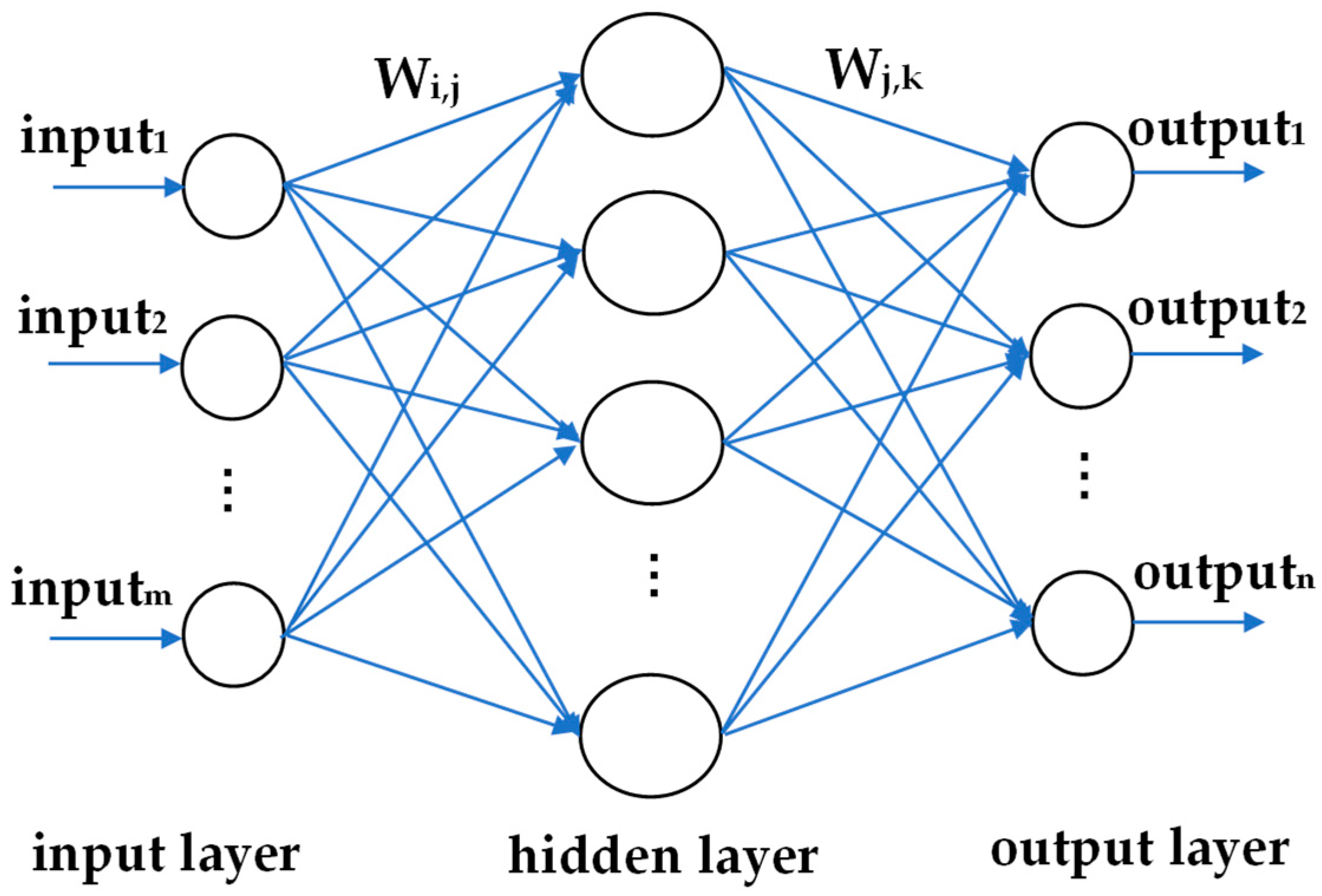
The back propagation neural network (BP neural network) is the most widely used neural network at present. Theoretically, a three-layer feedforward network can realize continuous function mapping with arbitrary accuracy, so a BP neural network can be effectively used to approximate a complex nonlinear function. As Figure 1 shows, a BP neural network consists of nodes at different levels, the output of nodes at each level is sent to the nodes at the next level. The output value is amplified or suppressed due to different connection weights. The excitation output value of each node is determined by the input excitation function and offset of the node [12].
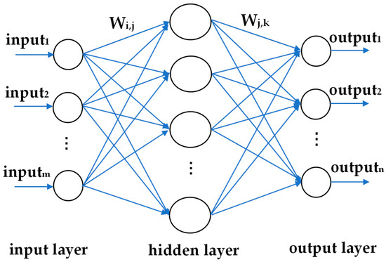
Figure 1.
Neural network structure diagram.
In Equation (1), , and are the number of nodes of the input layer, output layer and hidden layer, respectively.
2.2. PCA Spectral Reconstruction Technology
The difficulty in applying ANN technology to simulate spectra is that taking high-resolution absorption spectra as the output of ANN can lead to an excessive number of output nodes, which is a typical non-positive problem in fitting [13], and the training process may be drawn out simultaneously. Therefore, this paper introduces PCA spectral reconstruction technology. Principal component analysis (PCA) is a common method for feature extraction [14]. PCA projects the original data set into the feature space composed of the preferred feature vectors to achieve the purpose of representing the original high-dimensional data with low-dimensional data.
is a matrix composed of spectral data, and Equation (2) represents the singular value decomposition of R. In Equation (2), represents the number of samples, represents the fixed number of spectral channels (number of dimensions), and represents the number of principal components. is a diagonal matrix composed of singular values (SV) in descending order. Equation (3) represents the reconstruction of the matrix by the first NPC principal components, the matrix (loading matrix) is composed of the eigenvectors corresponding to the eigenvalues, and represents the low-dimensional matrix after dimension reduction. To quantitatively understand the numbers of PCs we need in PCA, we define a normalized cumulative SV (NCSV) as the ratio of the sum of the first NPC singular values to the sum of the total singular value. The value of NCSV represents the proportion of the information contained in the first NPC principal components to the information contained in the original matrix.
This paper adopted absolute relative error (ARE) to represent accuracy, and its expression is the following:
is usually the original or measured value, while is usually the new or calculated value, and is the absolute relative error between them.
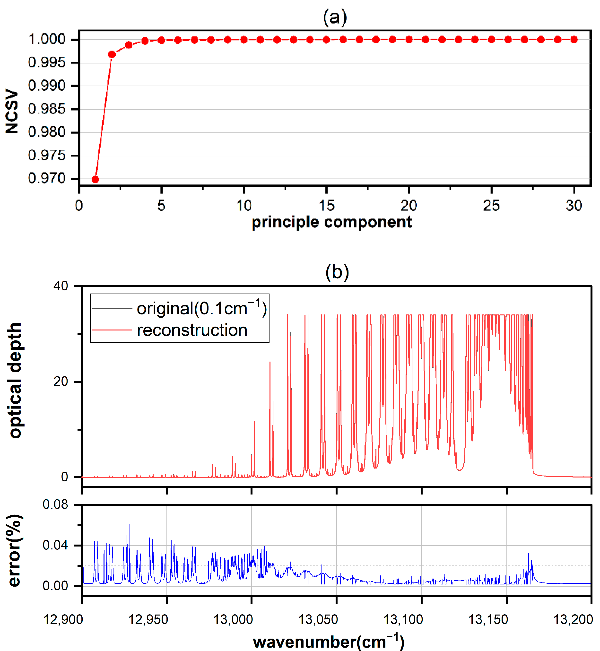
Figure 2a shows the relationship between NCSV and the number of PCs in the spectrum of oxygen A-band: under the spectral resolution of 0.1 cm−1, there are 3000 channels (3000 dimensions) in this band, the first 3 PCs have included more than 0.995 information of the original data and the first 10 PCs have included more than 0.99998 information of the original data.
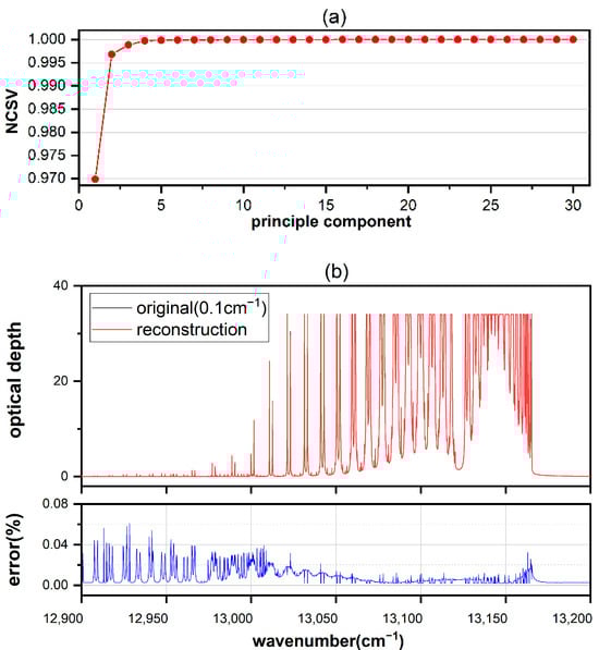
Figure 2.
Principal component analysis of oxygen A-band spectra. (a) Singular value for each principal component. (b) Normalized cumulative singular value as function of the selected number of PCs.
Figure 2b shows that in the case of taking the first 10 PCs, the absolute relative error between the spectrum reconstructed by Equation (3) and the original spectrum is between 0.002 and 0.08%.
3. Data Preprocessing and ANN Training Process
3.1. Applying ANN to Limb Observation Mode
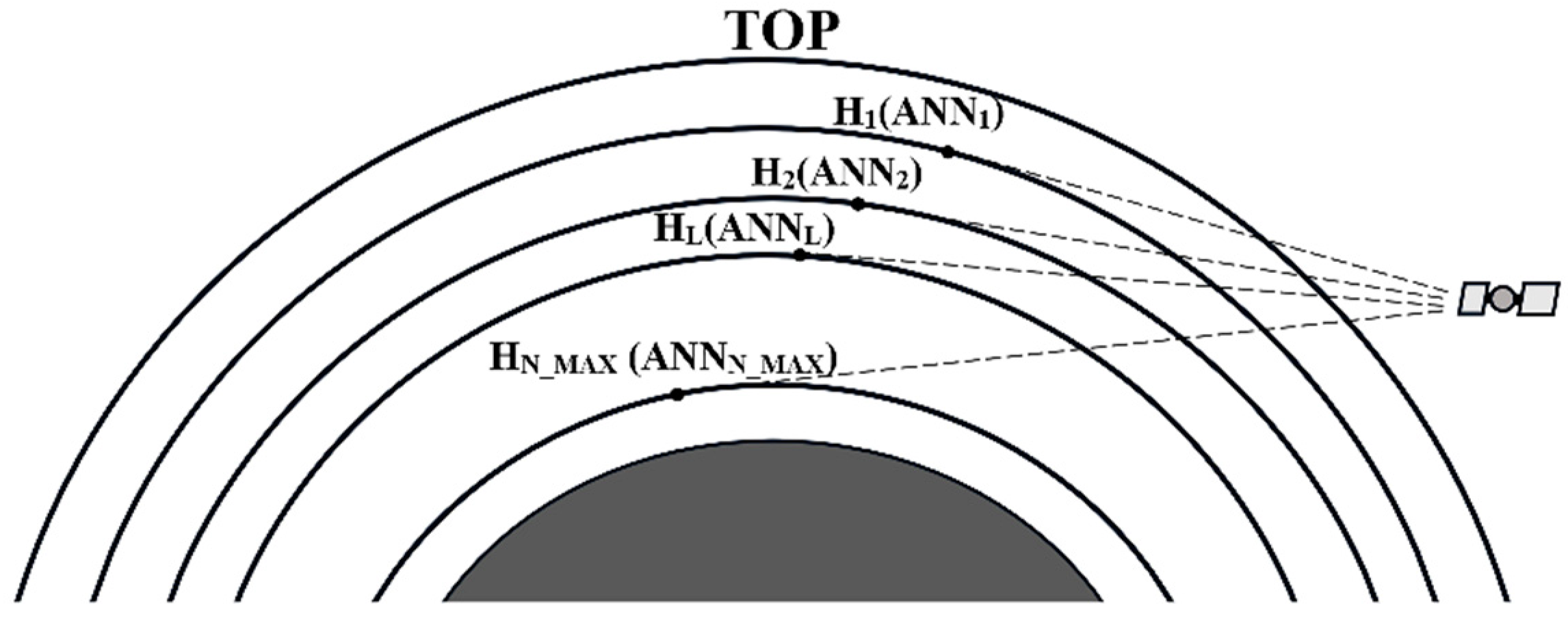
Figure 3 shows the limb observation mode. The height of the limb scanning tangent point from high to low is H1, H2… HL… HN_max and the subscript L represents the number of layers between the tangent point and the top of the atmosphere. The difficulty in using ANN to simulate limb atmospheric absorption spectra is that the number of parameters required for calculating limb spectra depends on the number of atmospheric layers above the tangent height. Therefore, it is not possible to use a single neural network to simulate limb spectra of different layers of the atmosphere; it is necessary to use a set of neural networks instead of one single neural network, namely ANN1, ANN2… ANNL… ANNN_max: ANNL is the neural network corresponding to the L-layer atmosphere below the atmospheric top. After training, when calculating the limb absorption spectrum at a certain tangent height, it is only necessary to know the number of atmospheres from the tangent height to the top of the atmosphere, and then select the ANN trained accordingly.
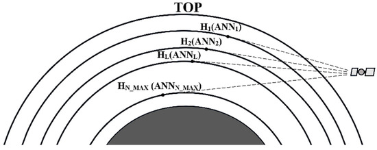
Figure 3.
Limb observation model.
N_max is the maximum sequence number of ANNs, representing the largest number of atmospheric layers that the ANNs can cover. The vertical resolution generally varies within a fixed range and the higher vertical resolution means more atmospheric layers, so the appropriate value of N_max is essential to meet the numerical simulation of most limb observation tasks.
3.2. Application to Simulations of GOMOS
GOMOS is a limb star occultation detector mounted on the ENVISAT satellite with an effective detection altitude of about 15–110 km. The detected wavelength spans from ultraviolet to visible rays, and the spectral resolution in the oxygen A-band (755–775 nm) is about 0.1 nm, which has a high spectral resolution compared to all other limb detectors in the same band. Its spectral data and atmospheric profile data are stored in GOMOS_Level1 and GOMOS_Level2 databases, respectively.
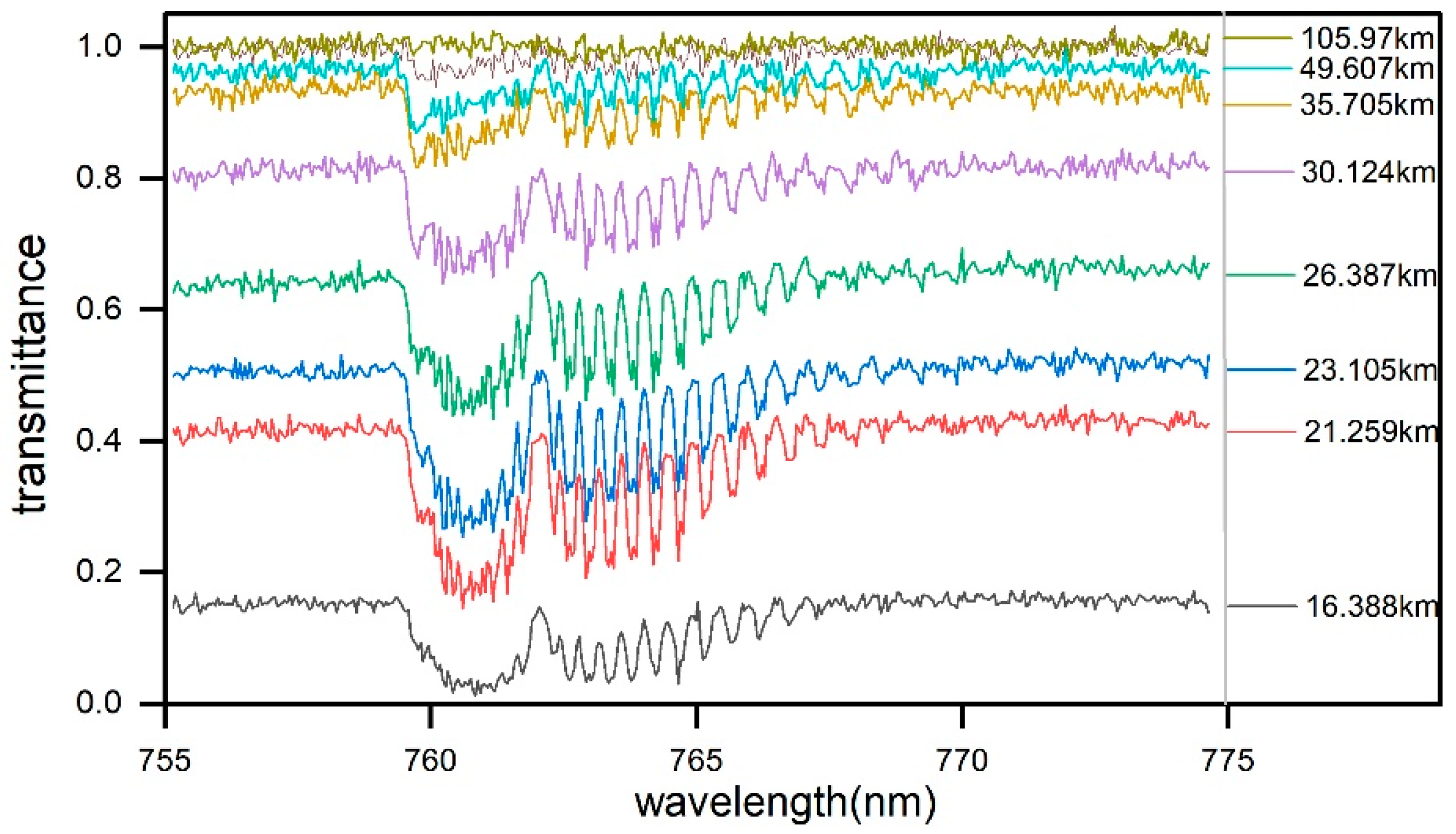
Figure 4 shows the limb absorption spectra detected by GOMOS within the oxygen A-band at different tangent heights. Compared to solar occultation, star occultation data have a lower signal-to-noise ratio, and noise has a major impact on detection data above the stratosphere (about 12~50 km), which can significantly affect the stability of inversion. Taking detection range and noise impact into consideration, this paper takes observing data in the stratosphere within the tangent altitude range of 15~50 km for training and inversion.

Figure 4.
GOMOS O2 A-band limb transmittance.
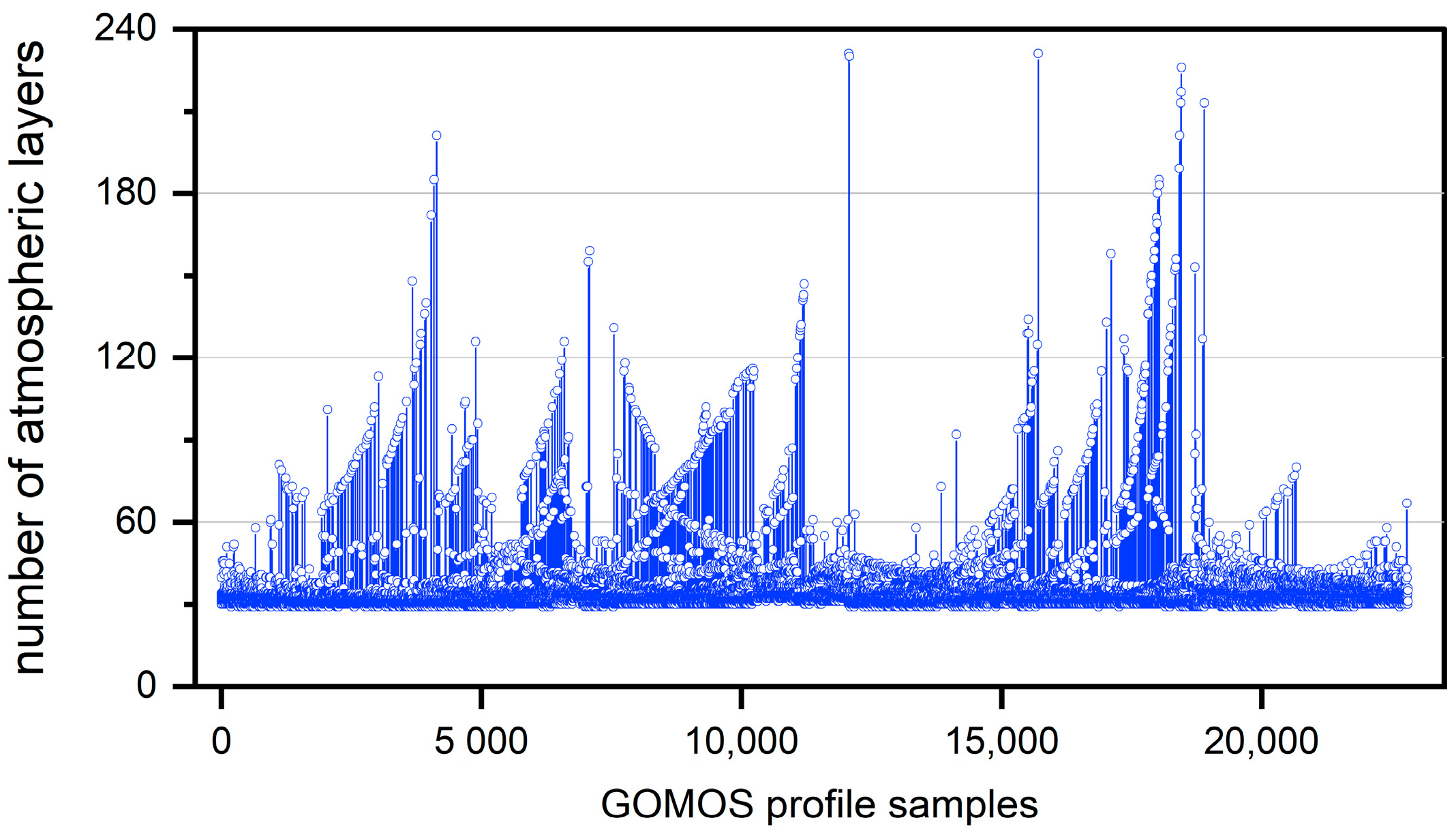
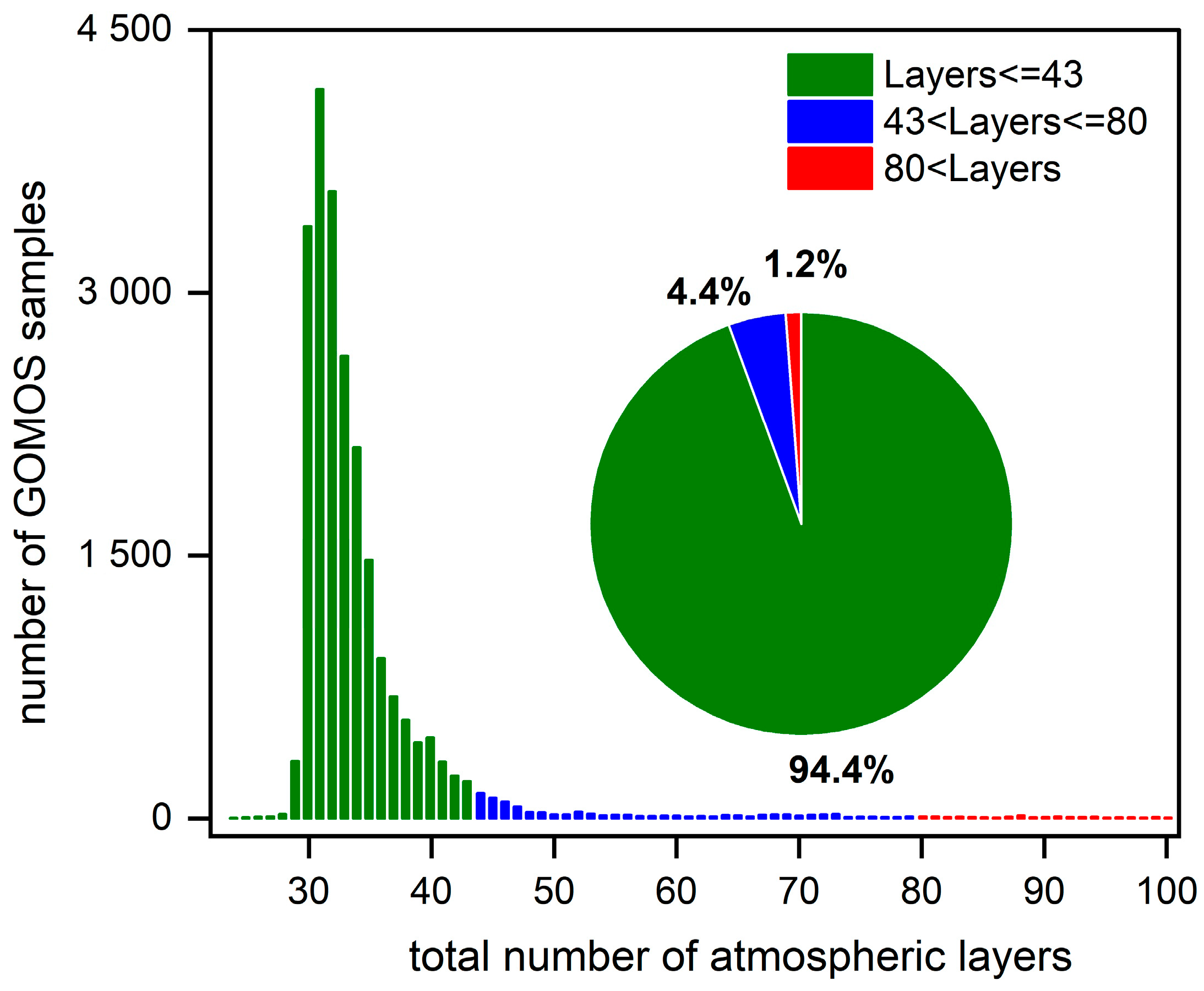
This paper conducted a random sampling on the data of GOMOS in 2003. Figure 5 shows the variation curve of the total atmospheric layers of limb scan samples in the range of 15~50 km. Figure 6 shows the sample distribution map of the total atmospheric layers. It can be seen that the sample distribution is mainly between 30~40 layers, with samples below 43 layers accounting for more than 94%. As the number of atmospheres increases, the increase in input terminals required for training neural networks leads to increased training difficulty. Simultaneously, noise also has an impact on high vertical resolution. Taking all factors into consideration, the maximum number N_max of atmospheres that the neural network can cover within the altitude range of 15–50 km is set to 43.

Figure 5.
Number of atmospheric layers in 2003.

Figure 6.
Statistics on the number of samples in different layers in 2003.
3.3. Establishing Training Databases
In order to train ANN1, ANN2, ANNL… ANNN_max, it is necessary to establish N_max corresponding databases (including input and output). The L layers below the top of the atmosphere have L + 1 boundaries. The input of the ANNL is the parameters on each boundary, including the corresponding density and the altitude of each boundary, with a total of 2 (L + 1) parameters. Using LBLRTM to compute atmospheric absorption spectrum at the corresponding tangent height, in order to better display the accuracy of the neural network calculation results, optical depth is used to replace transmittance to represent absorption spectra. The output of ANNs is the data obtained by PCA dimensionality reduction in the absorption spectra. Considering both accuracy requirements and training speed, the NPC (output node number) value is set to 10. In order to meet the accuracy requirements of this paper, each individual ANN requires a minimum of 5000 samples and is randomly assigned to the training set and testing set in a 9:1 ratio.
Table 1 shows the number of samples measured in 2003 corresponding to different L. It can be seen that when L > 30, the number of training and testing samples decreases sharply. Taking L = 43 as an example, it may take about a decade to obtain sufficient samples, and this obviously has no practical significance. In order to obtain sufficient training samples in a short period of time, it is necessary to re-layer the GOMOS profiles.

Table 1.
Number of GOMOS atmospheric samples corresponding to different atmospheric layers.
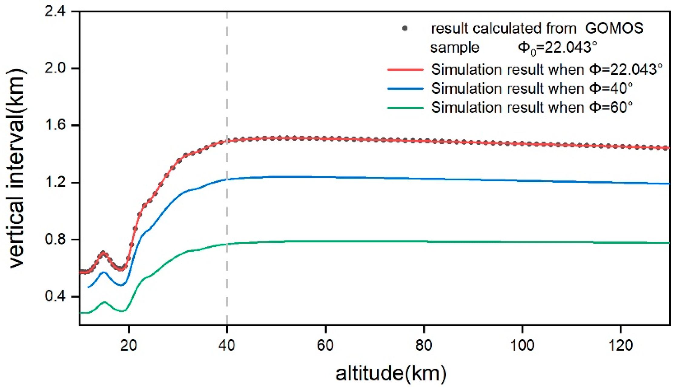
The observational time interval of GOMOS is fixed at 0.5 s, so the vertical resolution is just determined by the reference profile and the angle Φ between the incident ray and the orbit plane of the satellite [15], in which the reference profile mainly affects the vertical interval below 40 km through atmospheric refraction effects. To ensure the stability of the characteristics of GOMOS data, this paper uses variable Φ to re-layer atmospheric samples. As Figure 7 shows, black scatter plots represent the vertical interval directly calculated from GOMOS tangent height data and the official value of Φ is 22.043°, and the red curve represents the simulation results under the same reference profile and Φ condition. The two results are highly consistent, and the green and blue curves show the results after changing Φ to 40° and 60°. The results indicate that as Φ increases, the number of atmospheric layers and vertical resolution increase as the interval decreases.
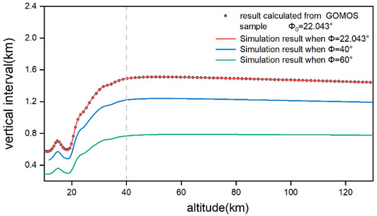
Figure 7.
Vertical interval of GOMOS.
3.4. ANN-HASFCM Modeling Process
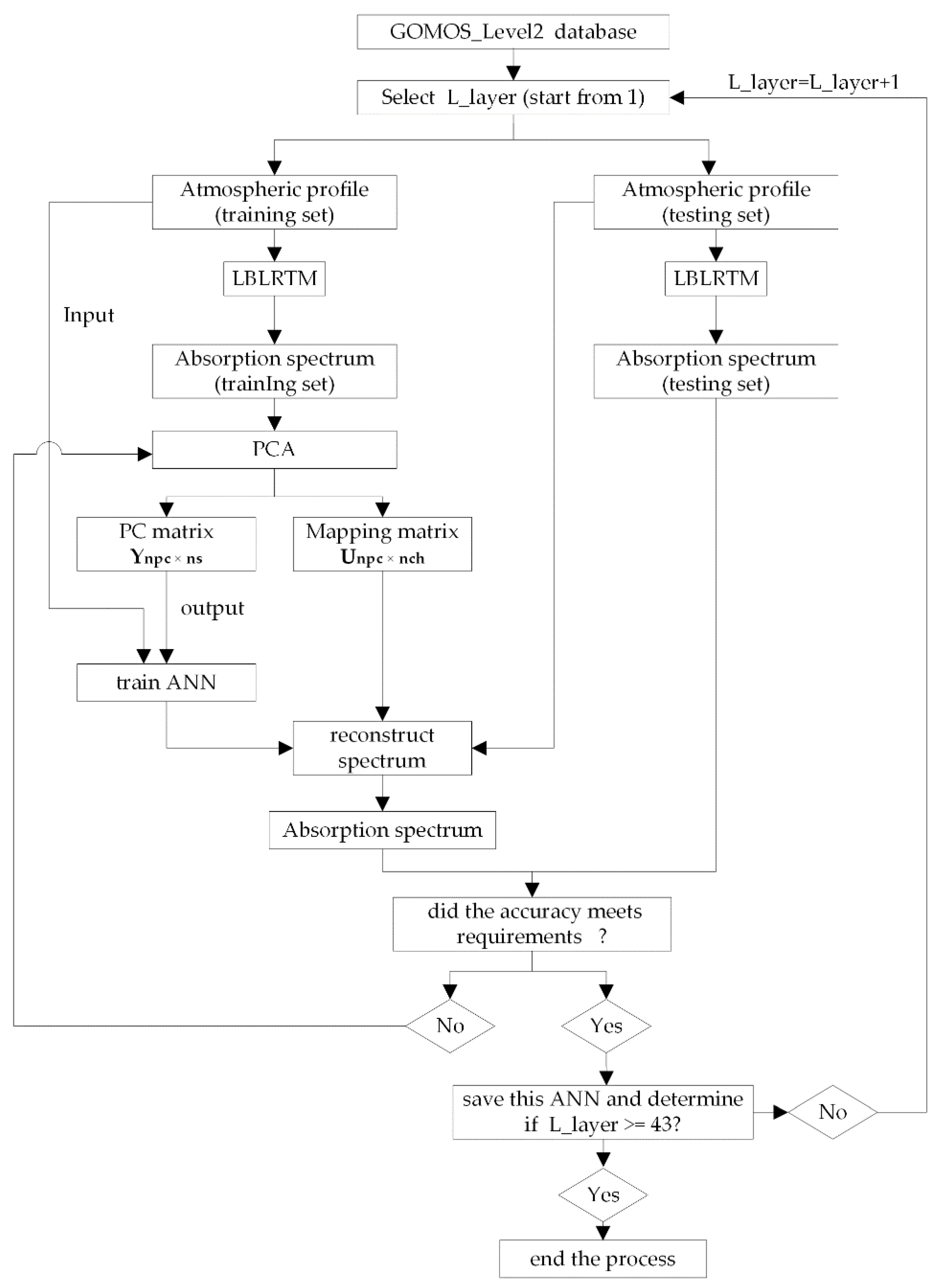
Figure 8 is the flow chart of the ANN-HASFCM modeling process; it describes all the details from selecting samples from the beginning to completing training at the end, which can be roughly divided into 5 steps.
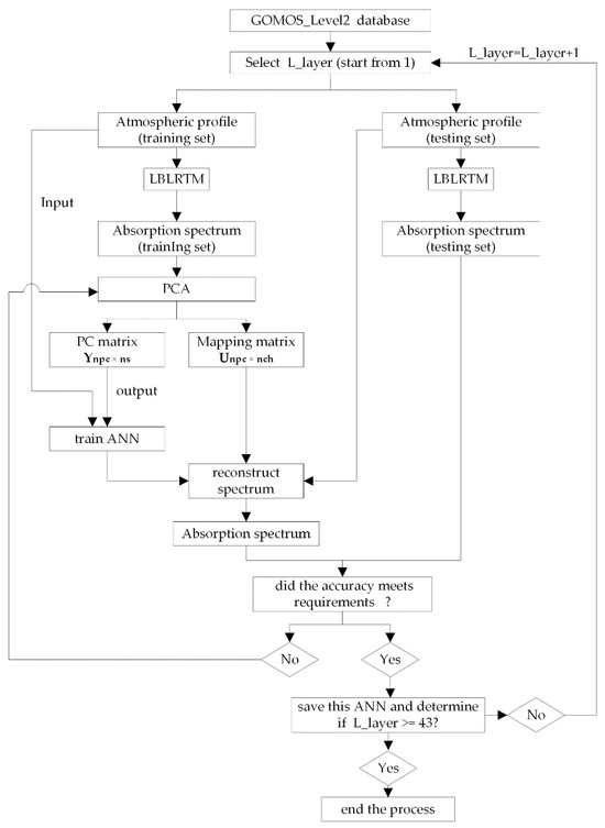
Figure 8.
Flow chart of ANN absorption spectrum fast computing model.
Step 1: Select atmospheric profile samples corresponding to the number of layers from the GOMOS_Level2 files to establish the ANN database, the number of layers starts from 1 and ends at 43. Then, use LBLRTM to generate the corresponding absorption spectra sample matrix R and establish the output database.
Step 2: The singular value decomposition is used to decompose the sample matrix R and sort the result in descending order of singular values:
Select the first NPC rows of the matrix as the mapping matrix and use the following equation to construct the principal component matrix .
Step 3: Use atmospheric parameters of the GOMOS level 2 database as the input data of ANNs and the principal component matrix as the output data, then randomly divide the data into training set and testing set, and start training.
Step 4: Use the trained neural network and the input data of the testing set to compute the output matrix and reconstruct the spectrum with the following equation:
Step 5: Verify the mean relative error between simulation values and test values; if the accuracy meets the requirements, save this ANN and the corresponding matrix U and perform the next ANN training until L_layer = 43. Otherwise, return to step 2 and reset the value of NPC and the related parameters of this ANN.
4. Computed Results
4.1. The Calculation Precision of ANN-HASFCM
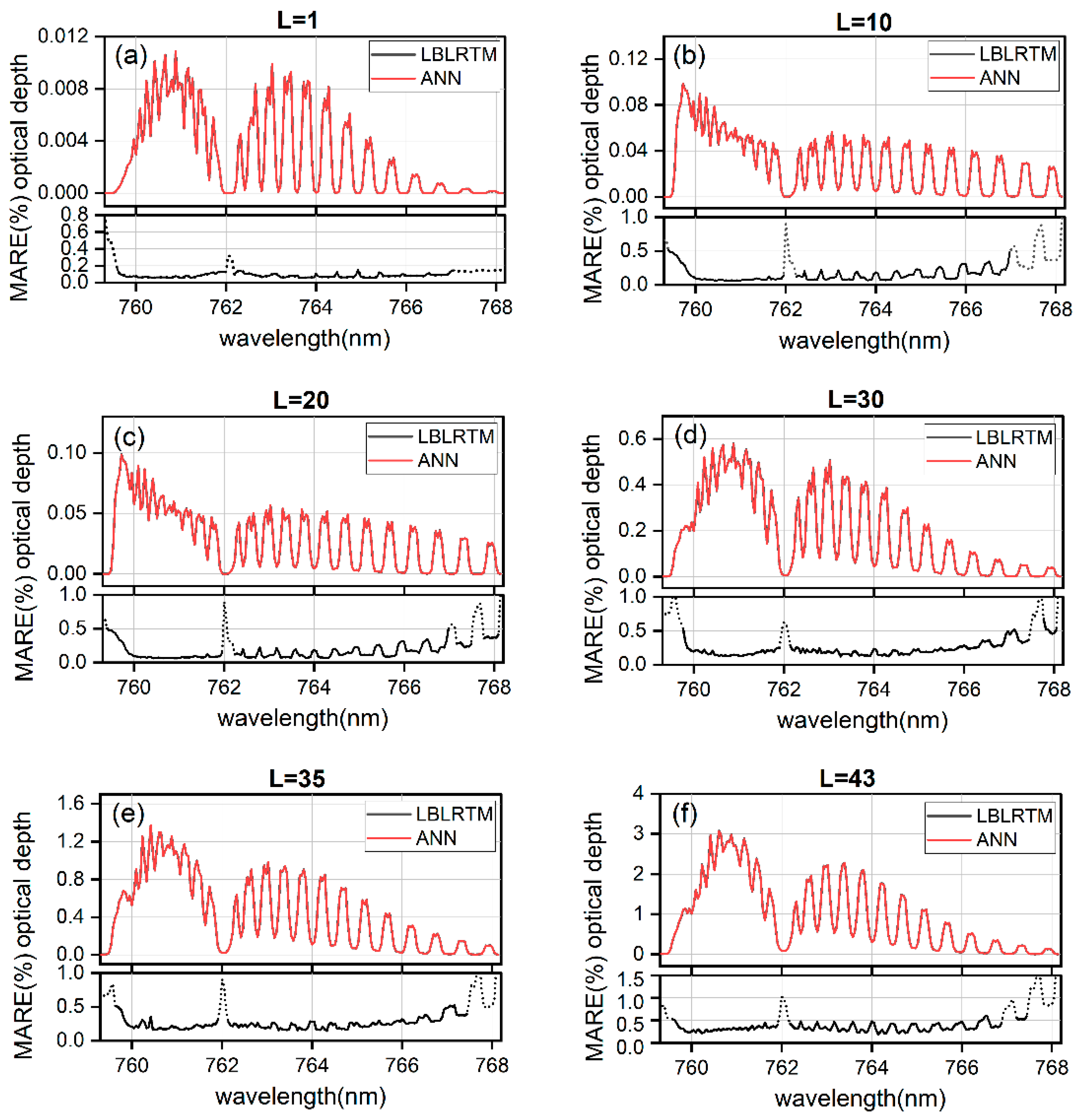
Figure 9 shows the computed results of limb optical depth spectra with ANN-HASFCM and LBLRTM for different atmospheric layers represented by L, and the calculation accuracy is represented by the mean absolute relative error (MARE) of the two models on the testing set calculation results.
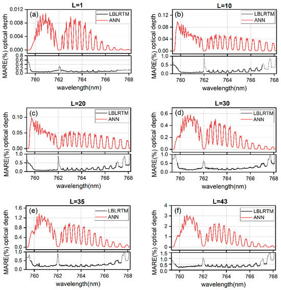
Figure 9.
ANN simulation results.
As shown in Figure 9, the calculation accuracy of ANN-HASFCM in the strong absorption band (black solid line) is between 0.03% and 0.65%, and the calculation accuracy of LBLRTM itself is about 0.5% [16], so the accuracy of ANN-HASFCM is equivalent to LBLRTM.
4.2. Inversion Accuracy of ANN-HASFCM
GOMOS officially uses a global-fitting algorithm to invert atmospheric profiles, which can effectively utilize all limb spectral information while avoiding the downward transmission of retrieval errors [17]. The general equation of its analytical solution is as follows [18]:
is the smoothing factor, which represents the strength of the smoothing constraint, is a regularization matrix and , as follows:
represents the number of iterations, is the calculated limb absorption spectra of all layers in the nth iteration, is the differential Jacobian matrix, is the error covariance matrix, which is a diagonal matrix calculated from the noise of each channel. is the pure oxygen molecular absorption spectra extracted by Differential Optical Absorption Spectroscopy (DOAS) [19]. We define n = 0 to represent the state before the iteration begins, so represents the priori atmospheric profile. , and can be obtained from the GOMOS_Level1 limb spectra database.
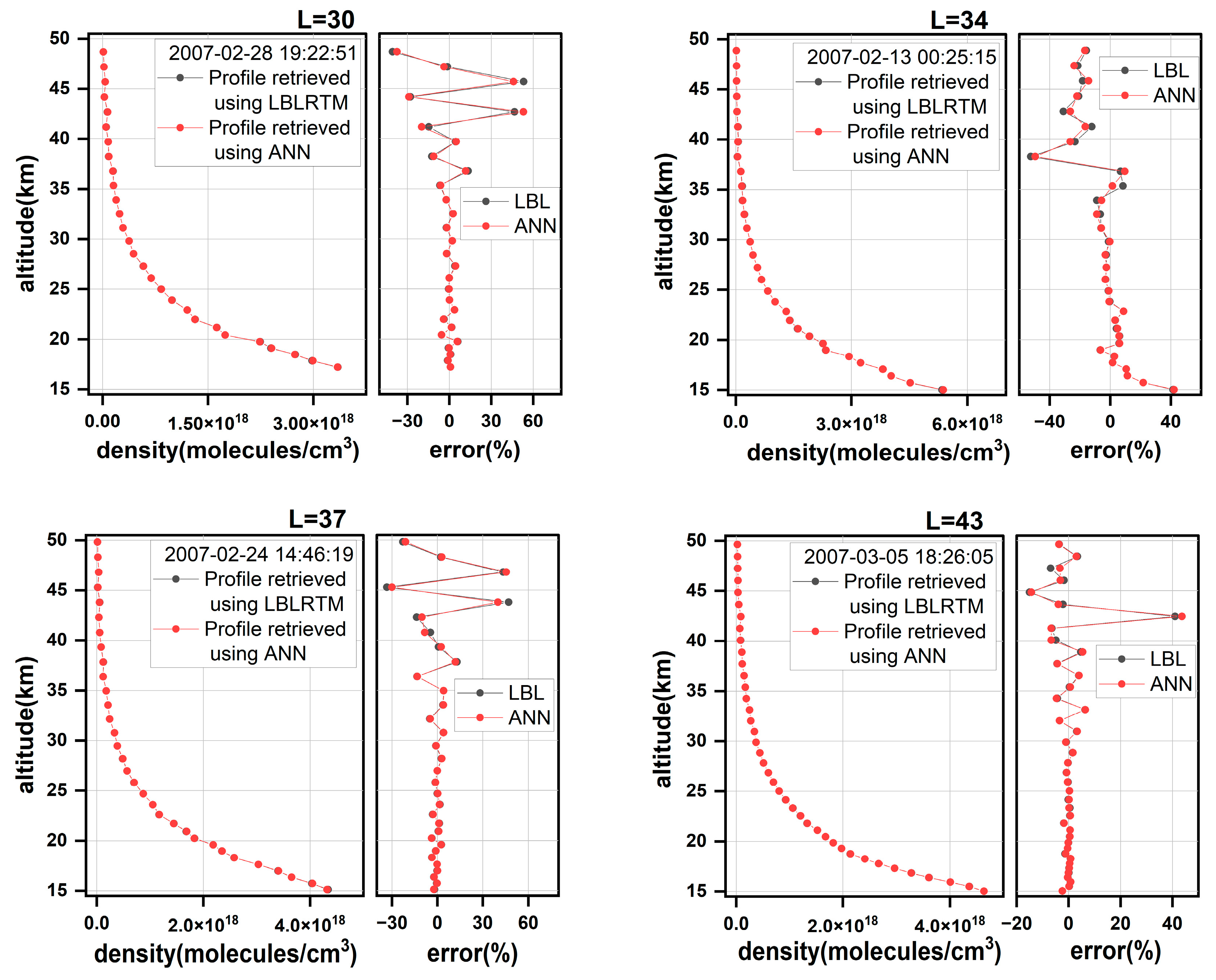
The measured samples of GOMOS in February 2007 are used as the target data to inverse, four atmospheric profiles with different vertical resolutions (represented by the total number of atmospheric layers L = 30, 34, 37 and 43, respectively) were randomly selected and the global-fitting algorithm was performed. As shown in Figure 10, LBLRTM and ANN-HASFCM were used as forward models, respectively, each graph presented the retrieval atmospheric density profiles within the range of 15–50 km, as well as the relative errors of posterior atmospheric density. It can be seen that the inversion results of LBLRTM and ANN-HASFCM are basically consistent.
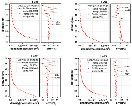
Figure 10.
Retrieval of atmospheric density profile.
4.3. Inversion Speed by Using the ANN-HASFCM in Global-Fitting Algorithm
Equation (6) is a general expression of inversion; its computation is mainly concentrated on and the Jacobian matrix , and the expression of in the global-fitting algorithm is determined by the following formula:
This paper calculates line by line, taking the jth row of the Jacobian matrix as an example:
In Equation (9), represents the derivative of the jth layer atmospheric absorption spectra to the ith layer atmospheric parameters. When using the traditional forward radiative transfer model for calculation, each layer of atmospheric density needs to be perturbed sequentially and then the perturbed atmospheric optical depth can be calculated. Considering when j > i, = 0, a total of L-j calculations are required. Even if the repeated calculation of some parameters is reduced, it is still time-consuming. When using ANN-HASFCM for calculation, due to the mapping relationship between the output and the input of ANNs, the perturbed atmospheric parameters of the L-j group can be used as inputs for simultaneous calculation. The total calculation time is equal to a single calculation, significantly reducing the inversion time.
In order to display the advantages of ANN-HASFCM in computation speed compared to traditional forward radiative transfer models, this paper uses Fast-LBLRTM as a reference to compare the computational speed of the two models. The following data are the average result of 20 repeated calculations. The main computer configuration of the computational environment is as follows:
- CPU: 2.10 GHz, AMD Ryzen 5 4600U with Radeon Graphics. The manufacturer is AMD(Advanced Micro Devices), an American fabless semiconductor company based in Santa Clara, California.
- OS: Windows 10, 64-bit operating system.
- Memory: 16 GB.
- Hard disk: SUMSUNG MZVLB5 12HBJQ-000L2. The manufacturer is Samsung Electronics, a Republic of Korean corporation headquartered in Yeongtong-gu, Suwon, Republic of Korea.
Table 2 shows the calculation time of for four different GOMOS atmospheric samples. The calculation time using Fast-LBLRTM as the forward model ranges from 8.443 s to 12.122 s, with an average calculation time of 0.273 s for each limb height. The calculation time using ANN-HASFCM as the forward model ranges from 0.295 s to 0.413 s, with an average calculation time of 0.00918 s for each limb height. The calculation speed is approximately 29.74 times faster.
Table 2.
Calculation time of .
Table 3 shows the calculation time of for four different GOMOS atmospheric samples. The calculation time of using Fast-LBLRTM as the forward model ranges from 121.361 s to 214.322 s. The calculation time of using ANN-HASFCM as the forward model ranges from 0.311 s to 0.42 s, and the calculation speed is approximately 382–508 times faster. It can be seen that due to the mapping characteristics of neural networks, their calculation time for and is basically the same. At the same time, the higher the vertical resolution of the atmosphere (with more layers), the more obvious the computational speed advantage of ANN-HASFCM.
Table 3.
Calculation time of .
5. Summary and Discussion
The ANN-HASFCM established in this paper simulates the absorption spectra of various limb paths in the altitude range of 15~50 km.
In terms of accuracy, compared with the accurate LBLRTM calculation results, the relative error in the oxygen A-band phase strong absorption channel does not exceed 0.65%, and some channels can be as small as 0.03%. As a forward transmission model, the inversion result with ANN-HASFCM has the same level of errors as with LBLRTM in the inversion of GOMOS limb spectra.
In terms of efficiency, the calculation speed of ANN-HASFCM is 20 times faster compared to traditional atmospheric radiative transfer models in calculating a single limb absorption spectrum, due to the characteristics of the global-fitting algorithm and the mapping characteristics of neural networks, the calculation speed of ANN-HASFCM in atmospheric inversion process is even faster. It can be predicted that ANN-HASFCM will have important applications in limb remote sensing.
With ANN-HASFCM as an application model, the training speed and stability should also be considered. From the analysis in Section 3.2, it can be seen that at present, ANN-HASFCM is able to complete 94.4% inversions of the data from the GOMOS detector, but to expand this proportion or for broader applications, it is necessary to increase the maximum number of atmospheric layers. As the number of input nodes increases, the training time and instability of ANN will also increase. The model can be further improved by optimizing the training procedure and parameters, and the machine learning technique itself. In the follow-up work, we plan to use a genetic algorithm to optimize the BP neural network for faster training speed and better stability. Genetic algorithms can realize the multipoint population search to avoid local optima and the optimization ability of genetic algorithms can also be utilized to obtain the optimal weights.
Author Contributions
J.Z. proposed and coded algorithms, processed all data and organized the manuscript. C.D. provided original suggestions and is the PI of the project. P.W. provided original purpose and funding support. H.W. reviewed and edited the manuscript and presented some suggestions. All authors have read and agreed to the published version of the manuscript.
Funding
National Key Research and Development Program of China, grant number 2019YFA0706004 and the Youth Innovation Promote Association CAS, grant number 2022450.
Data Availability Statement
Data underlying the results presented in this paper are not publicly available at this time but may be obtained from the authors upon reasonable request.
Acknowledgments
The authors would like to thank the (PI(s) and Co-I(s)) and their staff of the GOMOS project.
Conflicts of Interest
The authors declare no conflicts of interest.
References
- Wang, Y.; Sun, X.; Huang, H.; Ti, R.; Liu, X.; Fan, Y. Study on Influencing Factors of the Information Content of Satellite Remote-Sensing Aerosol Vertical Profiles Using Oxygen A-Band. Remote Sens. 2023, 15, 948. [Google Scholar] [CrossRef]
- Sugita, T.; Yokota, T.; Nakajima, T.; Nakajima, H.; Waragai, K.; Suzuki, M.; Matsuzaki, A.; Itou, Y.; Saeki, H.; Sasano, Y. Temperature and pressure retrievals from O2 A-band absorption measurements made by ILAS: Retrieval algorithm and error analyses. In Optical Remote Sensing of the Atmosphere and Clouds II; Society of Photo Optical: Bellingham, DC, USA, 2001; pp. 94–105. [Google Scholar]
- Stevens, M.H.; Englert, C.R.; Harlander, J.M.; England, S.L.; Marr, K.D.; Brown, C.M.; Immel, T.J. Retrieval of lower thermospheric temperatures from O 2 A band emission: The MIGHTI experiment on ICON. Space Sci. Rev. 2018, 214, 4. [Google Scholar] [CrossRef] [PubMed]
- Sheng, Z.; Huang, S.-X.; Fang, H.-X. Optimization the Inversion Model of Atmospheric Parameter Using Radio Occulation Data. J. Jishou Univ. (Nat. Sci. Ed.) 2004, 25, 10. [Google Scholar]
- Drouin, B.J.; Benner, D.C.; Brown, L.R.; Cich, M.J.; Crawford, T.J.; Devi, V.M.; Guillaume, A.; Hodges, J.T.; Mlawer, E.J.; Robichaud, D.J. Multispectrum analysis of the oxygen A-band. J. Quant. Spectrosc. Radiat. Transf. 2017, 186, 118–138. [Google Scholar] [CrossRef] [PubMed]
- Nowlan, C.R. Atmospheric Temperature and Pressure Measurements from the ACE-MAESTRO Space Instrument. Ph. D. Thesis, University of Toronto, Toronto, ON, Canada, 2006. [Google Scholar]
- Ovigneur, B.; Landgraf, J.; Snel, R.; Aben, I. Retrieval of stratospheric aerosol density profiles from SCIAMACHY limb radiance measurements in the O2 A-band. Atmos. Meas. Tech. 2011, 4, 2359–2373. [Google Scholar] [CrossRef]
- Bertaux, J.-L.; Kyrölä, E.; Fussen, D.; Hauchecorne, A.; Dalaudier, F.; Sofieva, V.; Tamminen, J.; Vanhellemont, F.; Fanton d’Andon, O.; Barrot, G. Global ozone monitoring by occultation of stars: An overview of GOMOS measurements on ENVISAT. Atmos. Chem. Phys. 2010, 10, 12091–12148. [Google Scholar] [CrossRef]
- Chuan, C.; Zheng, C.; Bo, L.; Ligang, L. Computation of atmospheric optical parameters based on deep neural network and PCA. IEEE Access 2020, 8, 102256–102262. [Google Scholar] [CrossRef]
- Le, T.; Liu, C.; Yao, B.; Natraj, V.; Yung, Y.L. Application of machine learning to hyperspectral radiative transfer simulations. J. Quant. Spectrosc. Radiat. Transf. 2020, 246, 106928. [Google Scholar] [CrossRef]
- Xiao, C.; Hu, X. Applying artificial neural networks to modeling the middle atmosphere. Adv. Atmos. Sci. 2010, 27, 883–890. [Google Scholar] [CrossRef]
- Gao, D.-Q. On structures of supervised linear basis function feedforward three-layered neural networks. Chin. J. Comput.-Chin. Ed. 1998, 21, 80–86. [Google Scholar]
- Tikhonov, A.N. On the solution of ill-posed problems and the method of regularization. Dokl. Akad. Nauk SSSR 1963, 151, 501–504. [Google Scholar]
- Liu, X.; Yang, Q.; Li, H.; Jin, Z.; Wu, W.; Kizer, S.; Zhou, D.K.; Yang, P. Development of a fast and accurate PCRTM radiative transfer model in the solar spectral region. Appl. Opt. 2016, 55, 8236–8247. [Google Scholar] [CrossRef] [PubMed]
- Kyrölä, E.; Tamminen, J.; Sofieva, V.; Bertaux, J.-L.; Hauchecorne, A.; Dalaudier, F.; Fussen, D.; Vanhellemont, F.; Fanton d’Andon, O.; Barrot, G. Retrieval of atmospheric parameters from GOMOS data. Atmos. Chem. Phys. 2010, 10, 11881–11903. [Google Scholar] [CrossRef]
- Feng, X.; Zhao, F.-S. Effect of changes of the HITRAN database on transmittance calculations in the near-infrared region. J. Quant. Spectrosc. Radiat. Transf. 2009, 110, 247–255. [Google Scholar] [CrossRef]
- Carlotti, M. Global-fit approach to the analysis of limb-scanning atmospheric measurements. Appl. Opt. 1988, 27, 3250–3254. [Google Scholar] [CrossRef] [PubMed]
- Nowlan, C.; McElroy, C.; Drummond, J. Measurements of the O2 A-and B-bands for determining temperature and pressure profiles from ACE–MAESTRO: Forward model and retrieval algorithm. J. Quant. Spectrosc. Radiat. Transf. 2007, 108, 371–388. [Google Scholar] [CrossRef]
- Stutz, J.; Platt, U. Numerical analysis and estimation of the statistical error of differential optical absorption spectroscopy measurements with least-squares methods. Appl. Opt. 1996, 35, 6041–6053. [Google Scholar] [CrossRef] [PubMed]
Disclaimer/Publisher’s Note: The statements, opinions and data contained in all publications are solely those of the individual author(s) and contributor(s) and not of MDPI and/or the editor(s). MDPI and/or the editor(s) disclaim responsibility for any injury to people or property resulting from any ideas, methods, instructions or products referred to in the content. |
© 2024 by the authors. Licensee MDPI, Basel, Switzerland. This article is an open access article distributed under the terms and conditions of the Creative Commons Attribution (CC BY) license (https://creativecommons.org/licenses/by/4.0/).