Retrieval and Comparison of Multi-Satellite Polar Ozone Data from the EMI Series Instruments

Abstract

The Environmental Trace Gases Monitoring Instrument (EMI) series are second-generation Chinese spectrometers on board the GaoFen-5 (GF-5) and DaQi-1 (DQ-1) satellites. In this study, a comparative analysis of EMI series data was conducted to determine the daily trend of ozone concentration changes owing to different transit times and to improve the overall quality and reliability of EMI series datasets. The daily EMI total ozone column (TOC) obtained using the Differential Optical Absorption Spectroscopy (DOAS) method were compared to vertical column density (VCD) gathered by the TROPOspheric Monitoring Instrument (TROPOMI). The results from October to November 2023 indicated a fine correlation (R = 0.98) between the daily EMI series data and a fine correlation (R ≥ 0.95) and spatial distribution closely resembling that of the TROPOMI TOCs. Furthermore, the EMI series data fusion results were highly correlated with TROPOMI TOCs (R = 0.99). Since the EMI series instruments had two different overpass times and the volume of available data at same pixel was increased by approximately three-fold, the temporal and spatial resolution was improved a lot. The results indicated that, compared to a single sensor, the EMI series DOAS TOCs generated more accurate and stable global TOC results and also enabled looking at the changes in the intraday TOCs. These outcomes highlight the potential of the EMI instruments for reliably monitoring the ozone variations in polar regions.

1. Introduction

As an important component of Earth’s atmosphere, ozone is a trace gas that can absorb the vast majority of shortwave ultraviolet (UV) radiation from the sun, thus protecting organisms from UV radiation damage [1,2]. In addition, ozone exhibits strong absorption in the infrared band centered on 9.6 μm; therefore, it is one of the greenhouse gases that produce a warming effect in the troposphere [3,4]. About 90% of ozone is distributed in the stratosphere at altitudes of 10–50 km and 10% is distributed in the troposphere below 10 km [5,6]; thus, ozone plays a crucial role in climate systems. Ever since Farman, Stolarsky, and their colleagues [7,8] identified the Antarctic ozone hole caused by significant ozone loss in spring in Antarctica, ozone has been the focus of the scientific community in the polar regions, which are relatively less affected by human activities and whose climate change better reflects global climate change trends [9]. The chlorinated fluorocarbons (CFCs) generated by anthropogenic emissions cause significant ozone loss in the Antarctic spring through the catalytic cycling of polar stratospheric clouds within polar vortices [10,11]. In 1987, the Montreal Protocol was signed to systematically eliminate CFCs [12,13,14,15]. As a result, the ozone levels over the Antarctic Pole are rebounding, signaling the beginning of ozone layer recovery [16,17].

Based on the long-term observation demand for the recovery of stratospheric ozone holes, satellite observations have the advantages of large-scale and continuous observation and can be used to estimate the global longwave radiation effects of ozone and quantify radiation forcing [18,19]. Satellite-based measurements of total ozone columns (TOCs) have promoted atmospheric research, such as exploring stratospheric dynamics, monitoring the ozone hole, and measuring the vertical profile on a global scale [20,21,22,23]. In addition, these measurements have played a crucial role in verifying the simulation results of the chemical models [24,25].

With improvements in instrument spectral resolution, radiometric performance, and spatiotemporal coverage, the payload of the same observation method needs to be continuously upgraded [26]. Satellite-based observation of ozone began with the Solar Back Ultraviolet (SBUV) and the Total Ozone Mapping Spectrometer (TOMS) in the 1970s [27,28]. The Global Ozone Monitoring Experiment-2 (GOME-2) series instruments on Metop-A, Metop-B, and Metop-C have a coarse spatial resolution of 80 × 40 km² and can provide global coverage within three days [29,30,31,32]. The Sentinel 5 precursor (S5P) satellite was launched in October 2017, facilitating research on atmospheric chemistry and regional pollutant monitoring [33,34]. The first-generation Environmental Trace Gases Monitoring Instrument (EMI) features a coarse spatial resolution of 13 × 48 km²; it was launched in May 2018 [35,36]. After that, with the launch of the second-generation EMI series instruments in 2021 and 2022 [37,38], multi-satellite comparison and fusion is meaningful for achieving the goal of the long-term stability of satellite global observations. The second-generation EMI series instruments feature a spatial resolution of 13 × 48 km².

As a crucial component of the EMI series instruments’ observations, precise TOC products are obtained using the Differential Optical Absorption Spectroscopy (DOAS) technique [38,39]. This classical technique, widely employed to retrieve the column density of trace gases, utilizes nadir-viewing satellite sensors [31,34]. The algorithm for retrieving the vertical columns of ozone mainly consists of three steps: derive the so-called slant column densities (SCDs), air mass factors (AMFs) calculations, and vertical column densities (VCDs) calculations [36,37]. The first-generation EMI ozone products and EMI-2 ozone products were retrieved and validated using the World Ozone and Ultraviolet Radiation Data Centre (WOUDC) dataset, with an average deviation of less than 10% [38,39]. However, the performances of EMI-DQ01 and EMI-GF5(01A) have not yet been verified, and the calibration of differences between the EMI series instruments is still required to obtain higher-quality TOC products.

In this study, the DOAS method was used to obtain TOC results from the EMI series instruments. Reliable ground-based observations were used for comparison and cross-verification between EMI ozone products. Next, weighted fusion correction was performed. In addition, we analyzed the changes in the TOCs in the morning and afternoon and improved the spatial resolution and precision of the EMI ozone products via weighted fusion. This approach is suitable for accurate long-term ground-based observations of the Antarctic atmosphere. The aim of this study was to evaluate the ozone retrieval performance of a new generation of EMI series instruments and to assess the consistency, accuracy, and stability of the different ozone data products generated using those EMI instruments. By doing that, we can use long-term stable EMI data to better monitor the diurnal change of ozone and analyze the mechanism of ozone change and the healing of ozone holes.

The rest of this article is organized as follows. Section 2 describes the EMI data used in this study. Section 3 explains the steps followed in the retrieval algorithm, which focuses on the parameter settings and the sources of different retrieval parameters for the EMI series sensors. Section 4 compares the inter-satellite consistency and stability of the EMI observations with those of the TROPOspheric Monitoring Instrument (TROPOMI). Based on the validation results of the ground-based data, the diurnal variation in the polar ozone TOC results was analyzed by comparing the retrieval results for different overpass times of the EMI instruments. Section 5 presents the conclusions of the study and discusses future work.

2. Data

The second-generation EMI series are Chinese imaging spectrometers on board the GaoFen-5 (GF-5) and DaQi-1 (DQ-1) satellites that are used to monitor atmospheric constituents such as O₃ and NO₂ and the properties of various other trace gases [35,36,37]. At present, a multi-satellite observation network of three satellites hosts the EMI series instruments: the Environmental Trace Gas Monitor EMI-GF5 (02) (launched in 2021), the Hyperspectral Integrated Observation Satellite Atmospheric Trace Gas Differential Absorption Spectrometer EMI-DQ01 (launched in 2022), and the Atmospheric Environment Satellite Ultraviolet Hyperspectral Atmospheric Composition Detector EMI-GF5 (01A) (launched in 2022).

The EMI series instruments orbit the earth 14–15 times per day, have a spatial resolution of currently 13 × 24 km² at nadir, and have a large swath of 2600 km [35,36,37,38]. The technical specifications for the spectral resolution, spectral range, overpass time, and other indicators of the three EMI instruments are listed in

Table 1. Technical specifications of the EMI-GF5(01A), EMI-GF5(02), and EMI-DQ01 instruments.

Parameters	EMI-GF5(01A)	EMI-GF5(02)	EMI-DQ01
Spectral range (nm)	UV1: 240–290	UV1: 240–290	UV1: 240–290
	UV2: 290–380	UV2: 290–380	UV2: 290–380
	VIS1: 390–530	VIS1: 390–530	VIS1: 390–530
	VIS2: 550–710	VIS2: 550–710	VIS2: 550–710
Spectral resolution	0.3–0.6 nm	0.3–0.6 nm	0.3–0.6 nm
Spatial resolution	13 × 24 km2	13 × 24 km2	13 × 24 km2
Field of view	114°	114°	114°
Reference spectrum	Monthly averaged solar spectrum	Monthly averaged solar spectrum	Monthly averaged solar spectrum
Overpass time	13:30 p.m.	10:30 a.m.	13:30 p.m.

.

TROPOMI is onboard the S5Psatellite, with an overpass time of 13:30 LST. TROPOMI TOC products have been extensively verified by satellite data and ground observation data, and the mean deviation and mean standard deviation between TROPOMI and ground TOC are within 2% and 5% [34]. The TROPOMI dataset, including the daily mean VCD product (source: https://s5phub.copernicus.eu/dhus/#/home; last accessed 10 May 2024), were compared to the EMI series retrieval results.

In addition, the WOUDC dataset (source: https://woudc.org; last accessed 10 May 2024) and the Reliable System data from the Systeme d’Analyse par Observations Zenithale (SAOZ) (source: http://saoz.obs.uvsq.fr/SAOZ-RT_2023.html; last accessed 12 June 2024) dataset were used to evaluate the performance of the EMI series TOCs.

3. Methods

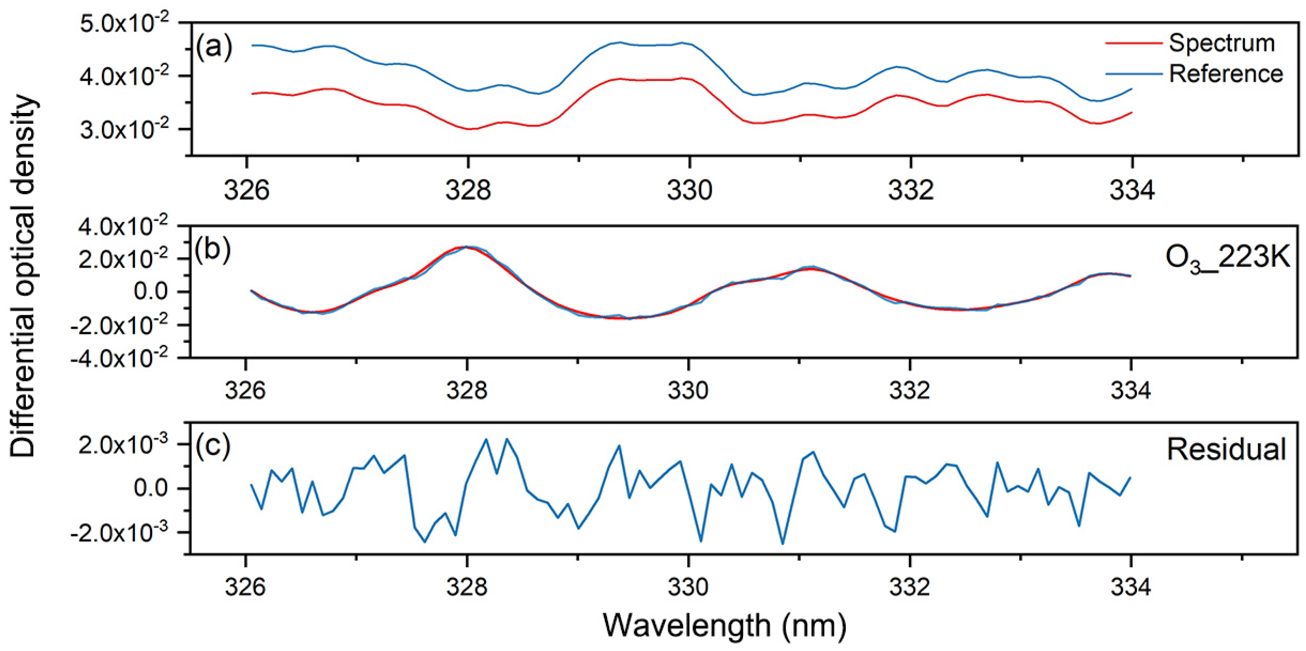
3.1. Deriving the Ozone Slant Column Density

The SCDs of atmospheric composition were retrieved using the DOAS technique, which is based on the Lambert–Beer law [40,41]. This method involves initially fitting the measured optical depths within a carefully selected spectral range to calculate the SCDs (integrated atmospheric concentrations along the effective light path) of the absorbers [42]. The basic equation describing the DOAS technique is [39]:

$$\ln {\displaystyle \frac{I\left(\lambda \right)}{I_o\left(\lambda \right)}}={\displaystyle \sum \left({\sigma }_i^{\ast }\left(\lambda \right)·c_i·L\right)={\displaystyle \sum \left({\sigma }_i^{\ast }\left(\lambda \right)·SC{D}_i\right)}}$$

(1)

where $I\left(\lambda \right)$ denotes the measured back-scattered earthshine intensity at wavelength $\lambda$, $I_o\left(\lambda \right)$ denotes the original solar intensity, $\ln {\displaystyle \frac{I\left(\lambda \right)}{I_o\left(\lambda \right)}}$ denotes the optical density, ${\sigma }_i^{\ast }$ denotes the cross section of trace gas $i$, $c_i$ denotes the concentration of trace gas $i$, $L$ denotes the optical path length, and the product of $c_i$ and $L$ defines the $SCD$.

In this study, we present the ozone SCD retrieval results of the EMI series, which were realized using version 3.2 of the QDOAS software program [43]. Through the DOAS retrieval residual fitting of the respective instruments, the wavelength intervals and polynomial fitting order with relatively low fitting root mean square (RMS) values are selected. Then, the retrieval parameters of the EMI series instruments were finally determined. The fitting intervals of the EMI-GF5 (01A), EMI-GF5 (02), and EMI-DQ01 were 320–340 nm, 326–334 nm, and 325–335 nm, respectively, and the polynomial fits were 4^th, 5^th, and 5^th order, respectively. The absorption cross sections were considered in the retrieval process.

Table 2. Detailed parameters of the ozone DOAS fitting for EMI-GF5(01A), EMI-GF5 (02), and EMI-DQ01.

Parameters	Source	EMI-GF5 (01A)	EMI-GF5 (02)	EMI-DQ01
Fitting interval		320–340 nm	326–334 nm	325–335 nm
Polynomial order		Order 4	Order 5	Order 5
${\mathrm{O}}_3$	223 K, 243 K (orthogonality) [44]	√	√	√
${\mathrm{N}\mathrm{O}}_2$	298 K [45]	√	√	√
${\mathrm{S}\mathrm{O}}_2$	298 K [46]	√	√	√
BrO	223 K [47]	√	√	√
HCHO	297 K [48]	√	√	√
Ring	Calculated using QDOAS	√	√	√

lists the parameter settings for the DOAS fit of the EMI series TOCs. A typical ozone DOAS fit for the EMI-DQ01 dataset is shown in Figure 1. The retrieved ozone SCDs and associated errors were approximately 7.157 × 10¹⁸ molecules/cm² and 2.841 × 10¹⁷ molecules/cm², respectively. The RMS values for the residuals of the spectral fit were 1.08 × 10⁻³.

3.2. AMF Calculation

The AMFs for the EMI series TOCs were determined using a look-up table (LUT) calculated with the SCIATRAN model [49]. The VCDs were derived from SCD/AMF values. These AMFs depend on observational geometry factors such as, relative azimuth angle (RAA), viewing zenith angle (VZA), surface albedo, solar zenith angle (SZA), cloud characteristics, and a priori ozone profile. TOMS V8 Climatology [50] provided the column-dependent ozone profile used as the a priori information.

In this study, the AMF was determined using multidimensional linear interpolation from a pre-calculated look-up table (LUT). For the EMI TOC, a two-step AMF calculation was employed. First, initial VCDs were derived from SCDs and rough AMFs, calculated using interpolation from a preliminary AMF LUT that excluded VCD as a parameter. The ozone profiles for this LUT were selected by month and latitude from the SCIATRAN database. Next, precise AMFs were calculated using interpolation from a detailed AMF LUT, which included the parameters listed in

Table 3. Parameters for node settings in the AMF LUT.

Parameters	Node	Values
Month	12	1, 2, 3, 4, 5, 6, 7, 8, 9, 10, 11, 12
Albedo	9	0, 0.05, 0.1, 0.20, 0.30, 0.40, 0.60, 0.80, 1.0
RAA (°)	5	0, 45, 90, 135, 180
Latitude (°)	18	−85, −75, −65, −55, −45, −35, −25, −15, −5, 5, 15, 25, 35, 45, 55, 65, 75, 85
SZA (°)	18	0, 10, 20, 30, 35, 40, 45, 50, 55, 60, 65, 70, 72, 74, 76, 78, 80, 82
VZA (°)	15	0, 5, 10, 15, 20, 25, 30, 35, 40, 45, 50, 55, 60, 65, 70
Cloud pressure (hPa)	9	1013, 795, 701, 616, 472, 356, 264, 164, 96
VCD (DU) for AMF correction	10	125, 175, 225, 275, 325, 375, 425, 475, 525, 575

[39].

4. Results and Discussions

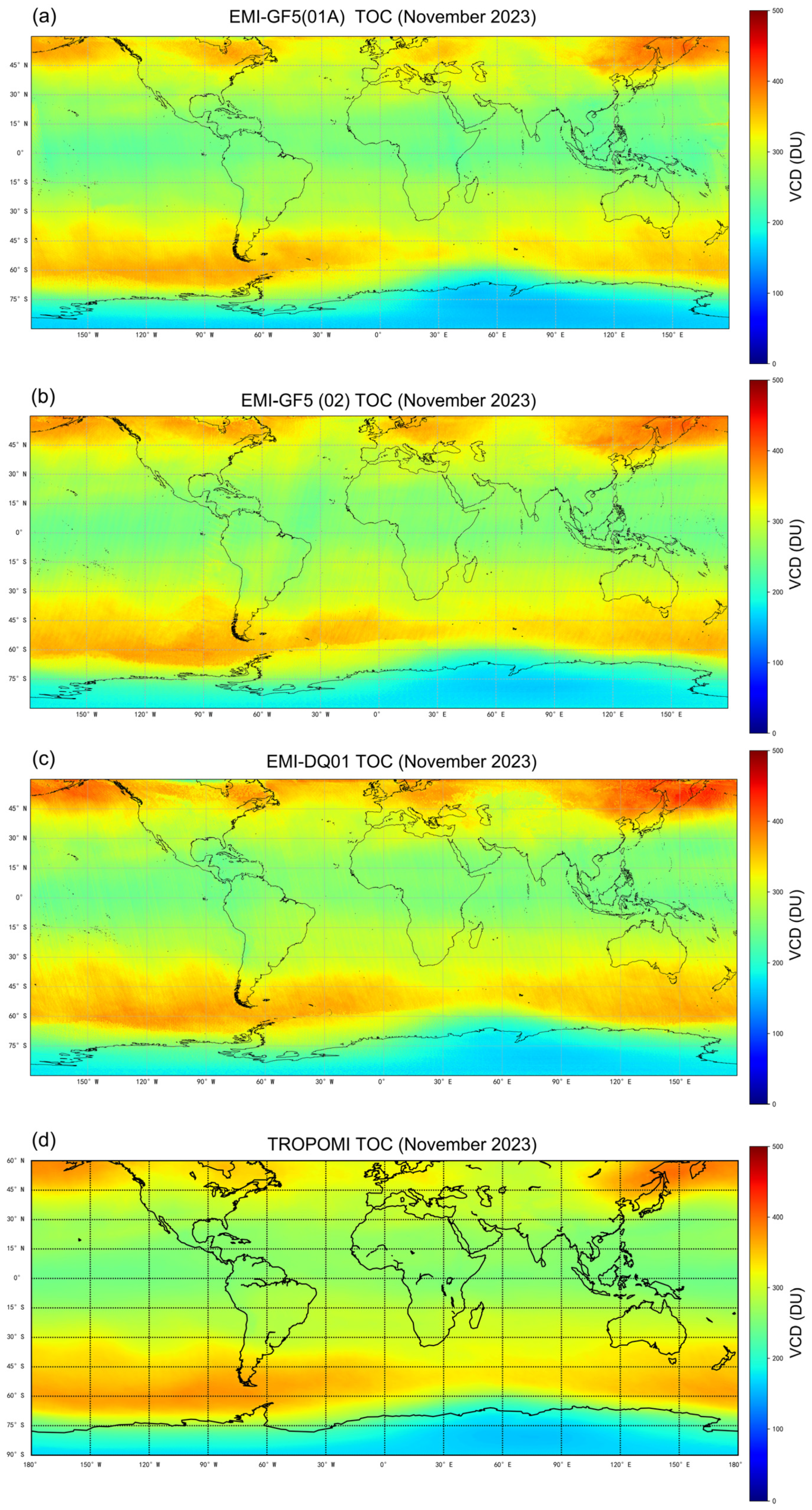
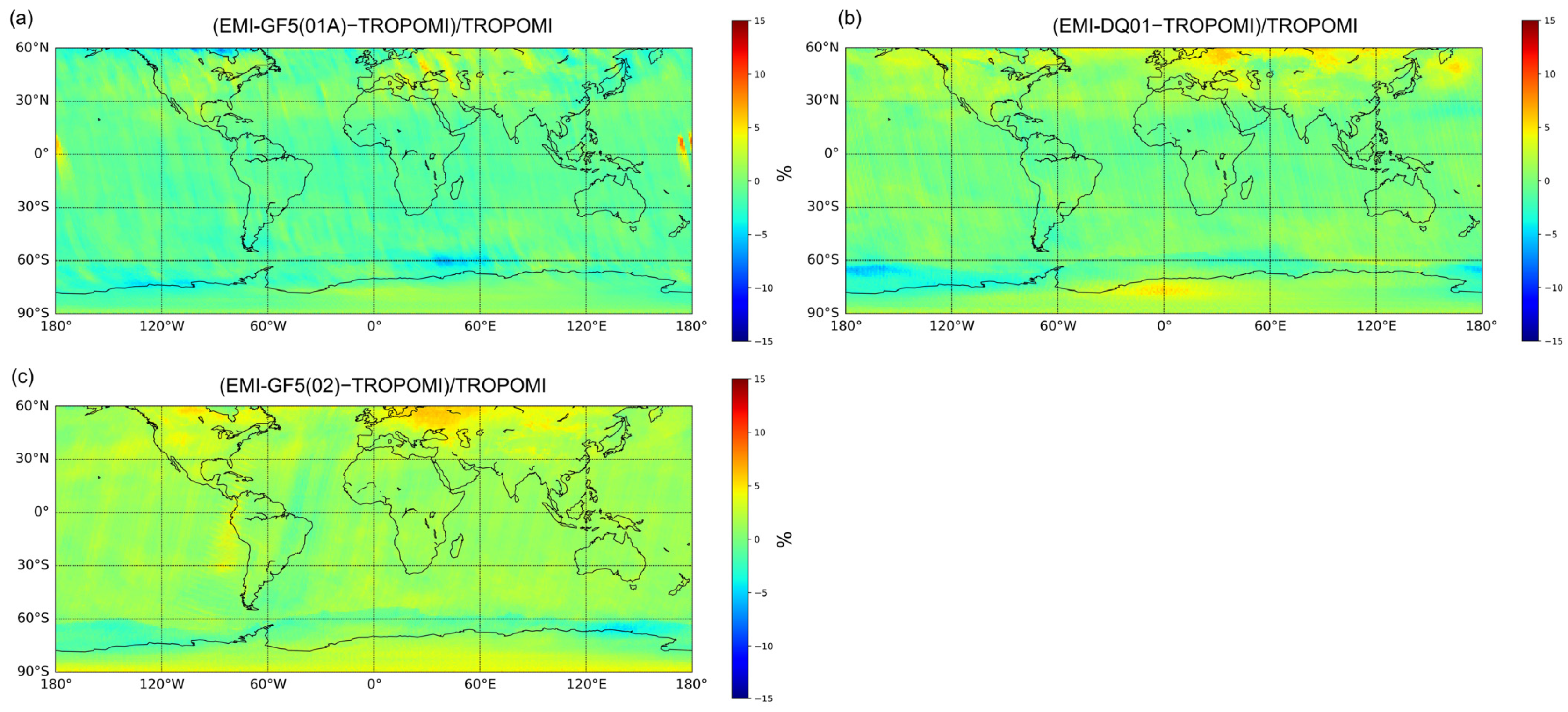
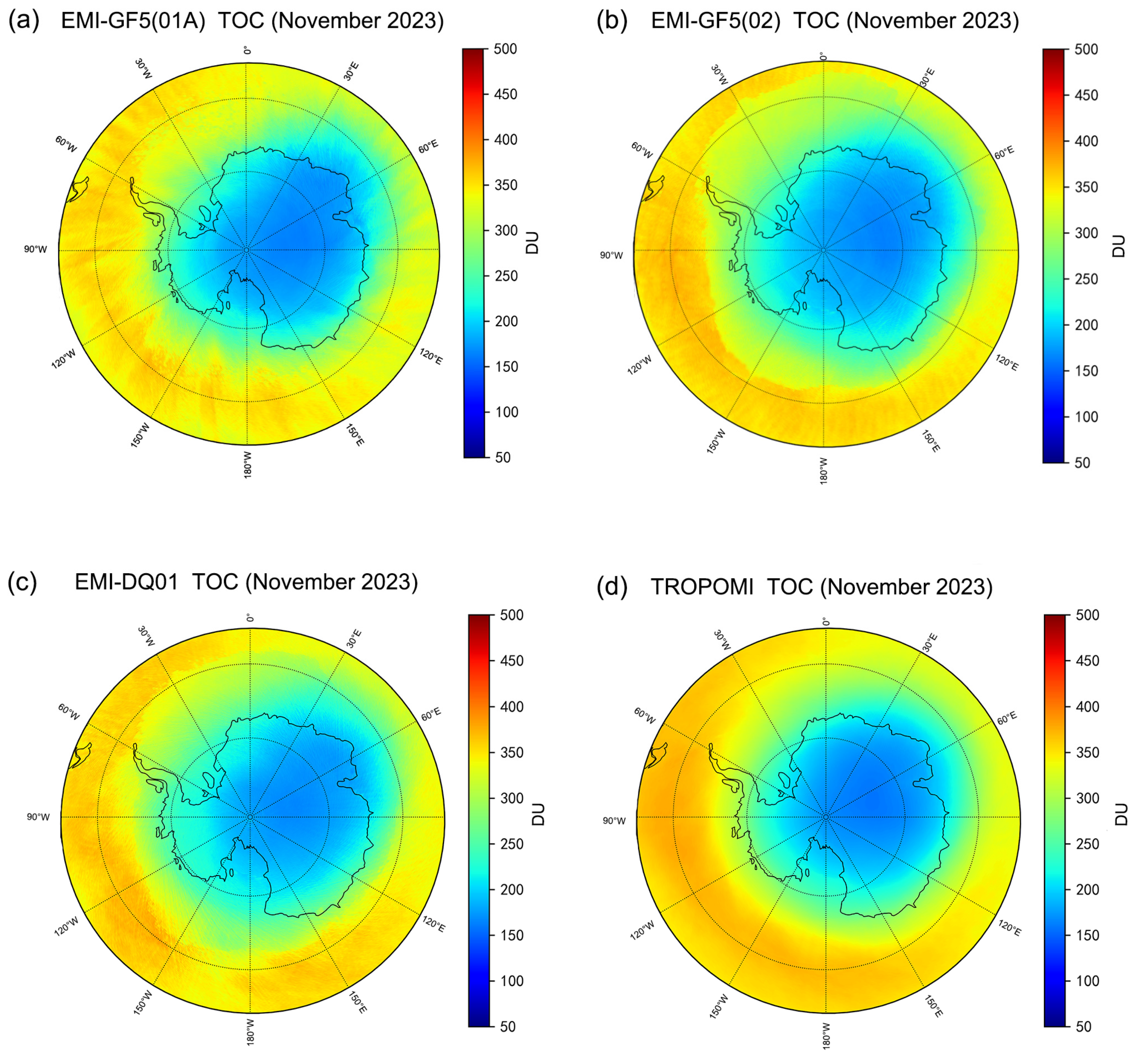
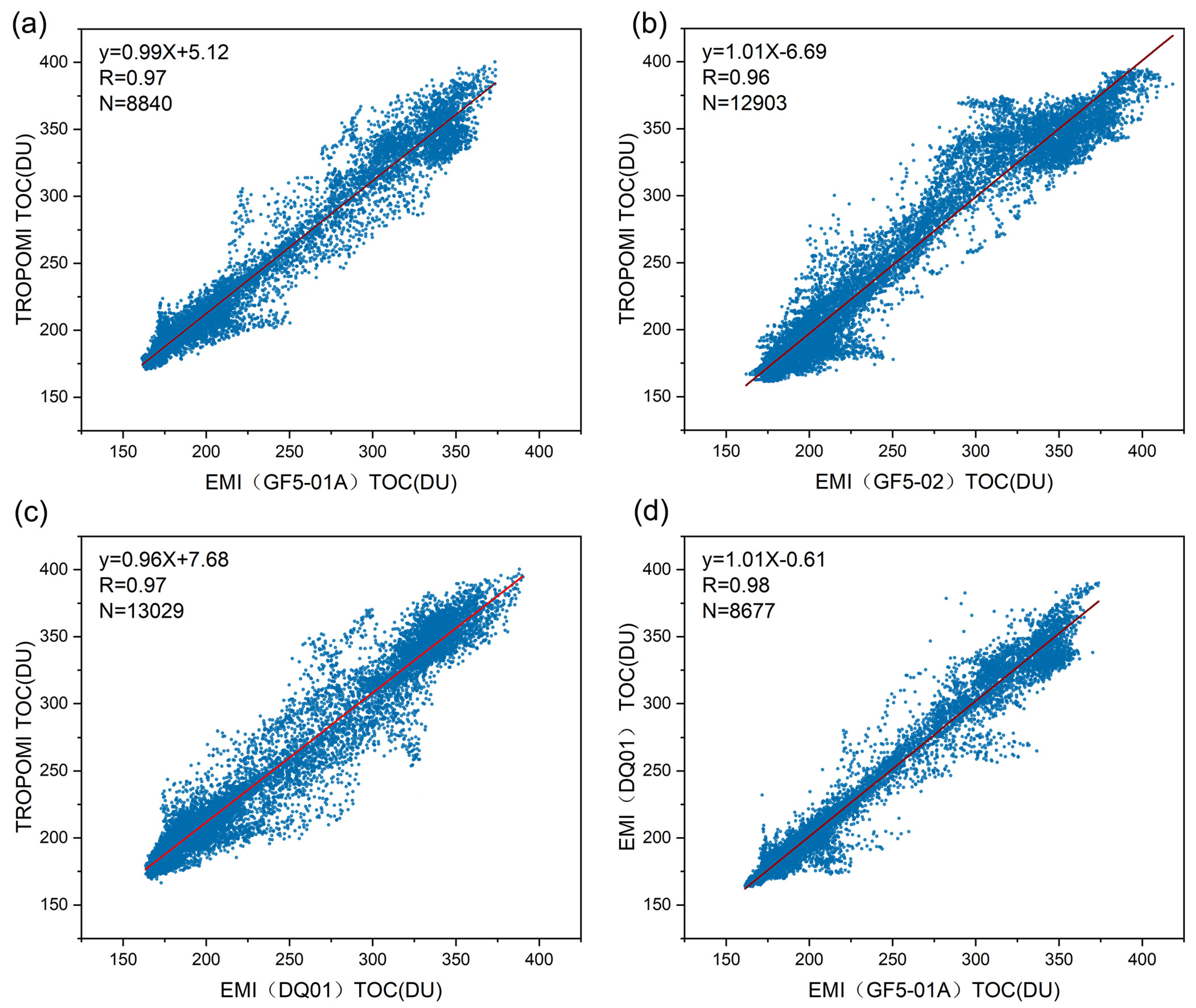
4.1. Comparison between Multi-Satellite Total Ozone Columns

Figure 2 shows the spatial distributions of the monthly mean global TOCs derived from the EMI-DQ01, EMI-GF5(01A), and EMI-GF5(02) instruments for November 2023. The capacity for monitoring changes in the global ozone distribution and the daily global coverage of the EMI series are shown in the figure. Figure A1 shows the daily spatial distributions of the EMI series and TROPOMI datasets for Antarctica (60°S–90°S latitude belts), which show an application example for analyzing the variation of the Antarctic ozone hole through EMI series measurements. Figure 3 shows the global maps of relative differences between EMI-GF5(01A), EMI-DQ01, and EMI-GF5(02) and TROPOMI TOC. Generally, the total ozone columns from the EMI and TROPOMI instruments show strong agreement, particularly in low- and mid-latitude regions. In comparison to the TROPOMI TOC, the EMI-GF5(01A) TOC exhibits a slight negative bias, with mean differences consistently below zero. However, these differences are generally less than −3% in both low- and mid-latitude regions. In addition, the Antarctic TOCs for the EMI series instruments had a resampled spatial resolution of 0.25° × 0.5° (latitude × longitude). As shown in Figure 2 and Figure 4, high ozone values were concentrated between 30 and 60°S, while low ozone values were evident in the regions of Antarctica.

The EMI series TOCs shown in Figure 2a–c are very similar to the overall spatial distribution of the TROPOMI TOCs shown in Figure 2d. This indicates that the EMI instruments have the capability of stably monitoring the Antarctic ozone hole on a daily basis. Figure 2 indicates that in the low and high latitudes of Antarctica, the ozone values were high and low, respectively, reflecting the daily variation of the ozone hole. In addition, the spatial distributions of TOCs in the EMI series datasets were highly consistent, which verified the stability of the EMI observations. This also provides a basis for mutual verification between EMI series instruments.

The monthly average Antarctic TOC results of the EMI-DQ01, EMI-GF5(01A), and EMI-GF5(02) datasets for November 2023 are shown in Figure 4. During this period, the overall spatial distributions of the EMI-DQ01, EMI-GF5 (01A), and EMI-GF5(02) TOCs were very similar, with an average relative deviation of approximately 0.18%, indicating that the EMI observations were stable and consistent. The monthly mean TOCs of the EMI instruments (Figure 3a–c) exhibited an overall spatial distribution similar to that of the TROPOMI data (Figure 3), with an average relative deviation of approximately 0.18%. The mean relative difference between EMI-DQ01 and EMI-GF5(01A) TOCs is defined as:${\Delta }_{\mathrm{rel}}=100\%\times {\displaystyle \frac{\text{EMI-DQ}01-\text{EMI-GF}5\left(01\mathrm{A}\right)}{\text{EMI-GF}5\left(01\mathrm{A}\right)}}$.

As shown in Figure 4, the monthly EMI series mean relative difference of the overall means were 0.16%, 2.38%, and 2.58%, respectively. As shown in Figure 3, the average relative deviations between the EMI series TOCs and TROPOMI TOCs for the latitudes of 60–90°S were −1.78%, 3.38%, and 3.42%, respectively, with average standard deviations of 1.98%, 2.98%, and 3.58%, respectively. The average relative difference in the Antarctic was negative, whereas it was positive in the tropical regions. This may have occurred because of the difference between the results generated by the linearized vector discrete ordinate radiation transfer (VLIDORT) code and the scientific radiation transfer model constructed using the EMI TOCs.

However, at high TOC values, the EMI-DQ01 TOCs appeared to be slightly higher than the TROPOMI TOC values. The difference between the EMI-GF5(02) and TROPOMI datasets was relatively large because the overpass time of EMI-GF5(02) was in the morning, while that of TROPOMI was in the afternoon. This demonstrates that polar ozone TOC values with different overpass times are beneficial for analyzing the intraday variation in ozone and improving the temporal resolution of satellite-based observations.

The linear fits between the daily global TOCs of the EMI-GF5(01A), EMI-GF5(02), and EMI-DQ01 datasets and those of the TROPOMI dataset for 20 November 2023 are shown in Figure 5. And Figure A1 shows the daily spatial distributions of the EMI series and TROPOMI datasets for Antarctica (60°S–90°S latitude belts). The regression analysis shown in Figure 5d demonstrates that the EMI-GF5(01A) and EMI-DQ01 TOCs were highly correlated, with a Pearson’s correlation coefficient (R) of 0.98.

4.2. Ozone TOCs Diurnal Variations Analysis

Because of the different overpass times of the EMI series, we investigated the differences in the datasets to characterize the diurnal variations in the ozone TOCs. Figure 6 shows the overpass TOC values of the EMI-DQ01, EMI-GF5 (01A), and EMI-GF5(02) datasets at four ground stations from 20 November 2023 to 24 December 2023. The figure indicates that the EMI-DQ01 and EMI-GF5 (01A) datasets were consistent, with an average deviation of 0.58%. The results also showed that morning and afternoon variations in the ozone TOC values varied in different latitude regions. In high-latitude regions, daylight hours were shorter and ozone generation activity was relatively low. The morning and afternoon changes in the ozone concentrations were relatively stable. The average difference between the EMI-DQ01, EMI-GF5(01A), and EMI-GF5(02) datasets at Dumont station was 0.8%. In mid-latitude regions, the morning and afternoon variations in the ozone concentration were slightly large, with the average difference between the morning and afternoon datasets being 1.4%. At the low-latitude Reunion station, sunlight was strong during the day and ozone generation was more active. The concentration of ozone changed significantly in the morning and afternoon, with the average difference between the morning and afternoon datasets being 2.49%, since daylight conditions were more favorable for ozone generation.

Based on the retrieval results for the EMI series, the diurnal variations in the TOCs for different regions were analyzed; this process improved the temporal resolution of the EMI observations and can provide a reference for more refined detection of diurnal variations in ozone holes.

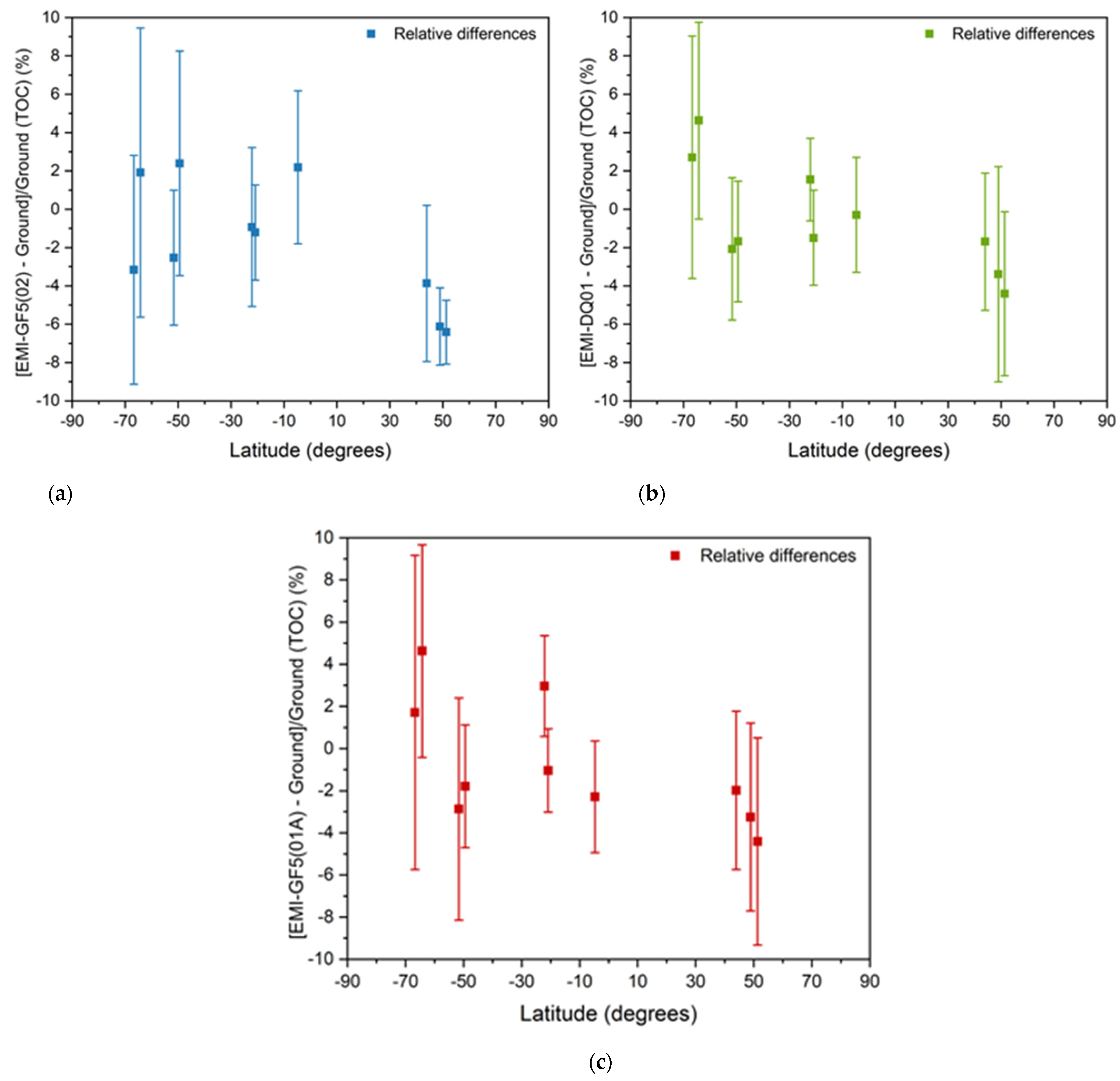
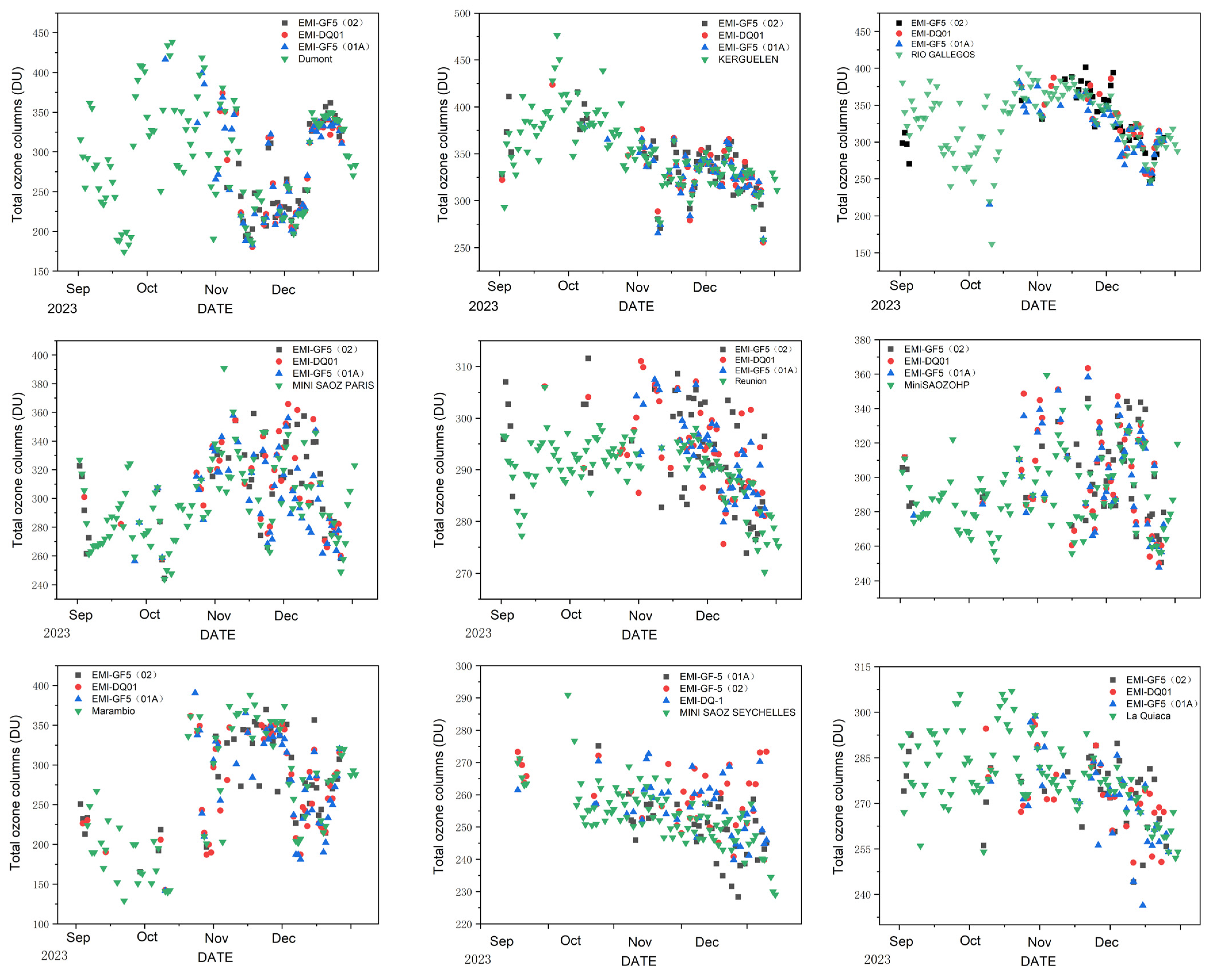
4.3. Validation with Ground-Based TOCs

The EMI DOAS TOCs were verified using reliable daily TOCs from several ground-based stations’ measurements in the WOUDC and SAOZ datasets. In this study, the TOC results for the daily average EMI data using the ground pixels (0.25° × 0.25°) of the corresponding ground-based stations were calculated. The relative differences between the EMI and ground-based TOC values are shown in Figure 7.

Table 4. Information on the stations and the mean relative differences between the EMI-GF5(01A), EMI-GF5(02), and EMI-DQ01 and ground-based TOCs.

Stations	Latitude, Longitude	Method	EMI-GF5 (02) Averaged Difference	EMI-GF5 (01A) Averaged Difference	EMI-DQ01 Averaged Difference
Reunion	20.9°S, 55.5°E	SAOZ	−1.21%	−1.05%	−1.49%
Rio Gallegos	51.6°S, 69.3°W	Dobson	−1.53%	−2.87%	−1.98%
Mini Saoz Paris	48.9°N, 2.3°E	SAOZ	−4.12%	−3.25%	−3.39%
Kerguelen	49.4°S, 70.3°E	Dobson	2.39%	−1.79%	−1.68%
Mini Saoz OHP	43.9°N, 5.7°E	SAOZ	−1.87%	−1.98%	−1.26%
TEH	51.32°N, 35.73°E	Dobson	−5.41%	−4.41%	−5.27%
Dumont	66.7°S, 140.0°E	SAOZ	−3.16%	2.71%	2.75%
Mini Saoz Seychelles	4.68°S, 55.53°E	SAOZ	2.19%	−2.99%	−4.54%
Marambio	64.23°S, 56.62°W	Dobson	2.79%	4.63%	2.72%
La Quiaca	22.11°S, 65.43°W	Dobson	0.93%	3.97%	1.55%

displays the average relative deviations observed between the EMI series and ground-based TOCs. Among them, EMI-DQ01 TOCs has the smallest deviation from the ground-based TOCs. The fluctuations between the EMI-GF5(02) and ground-based TOCs ranged from −5.41% to 4.12%, those between the EMI-DQ01 and ground-based TOC results ranged from −4.41% to 4.63%, and those between the EMI-GF5(01A) and ground-based TOC values ranged from −5.27% to 2.57%. The deviations were relatively large in high-latitude regions. The 2023 daily average standard deviations between the EMI-GF5(01A), EMI-GF5(02), and EMI-DQ01 and ground-based TOCs from September to December were 4.08%, 4.12%, and 3.94%, respectively. The above TOC results indicated the consistency and accuracy of the EMI TOC retrieval, with the maximum deviation being 4%.

Possible causes of biases could have been the different air masses probed by the space- and ground-based instruments. The a priori vertical profile information used in the retrieval algorithms may influence air masses. Information on the ten stations and the relative deviations are listed in Table 4, and the standard deviations are listed in

Table 5. Averaged standard deviation (std) between the EMI-GF5(01A), EMI-GF5(02), and EMI-DQ01 and ground-based TOCs.

Station	Emi-Gf5 (02) Averaged Std	EMI-GF5 (01A) Averaged Std	Emi-Dq01 Averaged Std
Reunion	2.48%	1.98%	2.48%
Rio Gallegos	3.52%	5.27%	3.71%
Mini Saoz Paris	2.01%	4.46%	5.61%
Kerguelen	5.86%	2.91%	3.15%
Mini Saoz OHP	4.07%	3.76%	3.58%
TEH	1.66%	4.91%	4.28%
Dumont	5.96%	7.45%	6.32%
Mini Saoz Seychelles	3.99%	2.65%	2.99%
Marambio	7.34%	5.04%	5.13%
La Quiaca	4.15%	2.39%	2.15%

. Figure 8 displays scatter plots comparing the time series of the EMI series and ground-based TOCs measured at several stations worldwide.

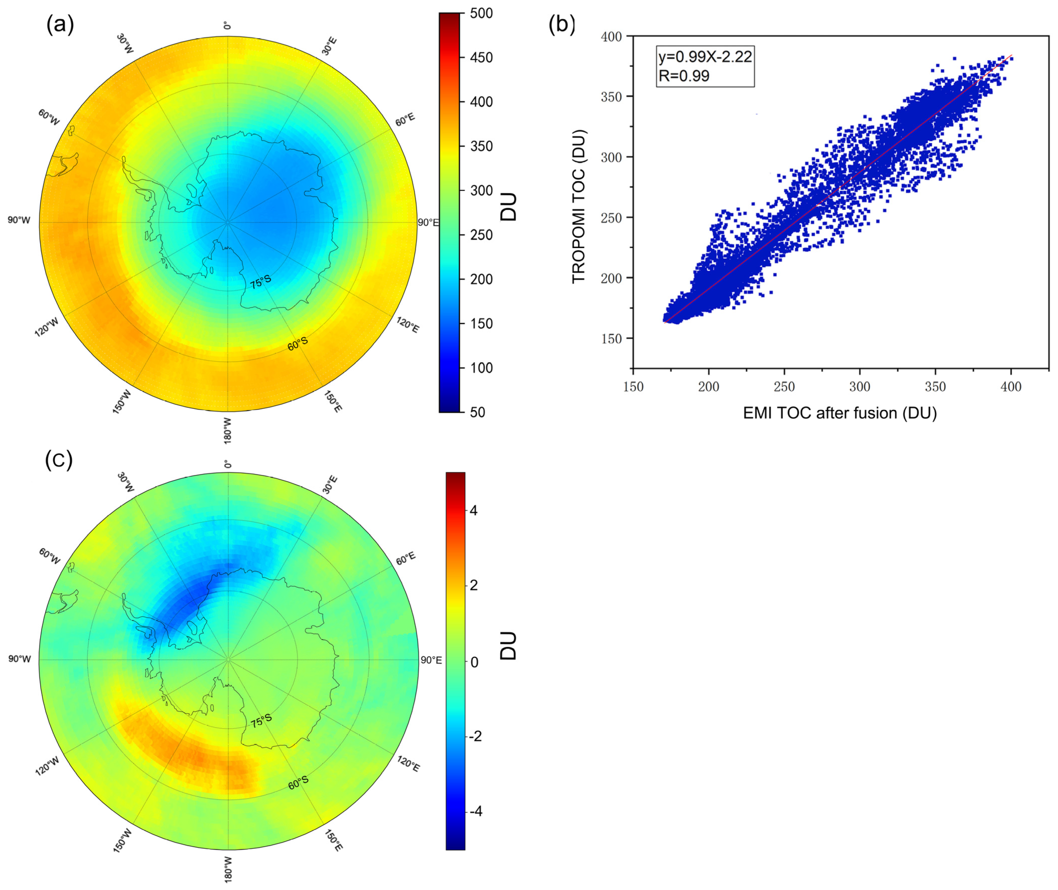
4.4. Weighted Fusion Correction

The results indicated that certain differences existed between the different EMI instruments, which could be attributed to many factors, including algorithms, data sources, and environmental conditions. In addition, the EMI instruments also occasionally have missing tracks. Therefore, it was necessary to explore suitable data fusion methods to reduce the random and systematic errors in the EMI instruments, improve the spatial coverage, and provide higher-quality TOC products. The weighted fusion of the spatiotemporal data provided the prospect of improving the spatial and temporal resolutions of the EMI series instruments. By assigning weighting factors to each instrument, weighted fusion could achieve an optimal data fusion [51]. Thus, we assigned weighting factors according to the RMS values of the different EMI instruments. RMS values are obtained by QDOAS retrieval for different EMI instruments, and EMI values with lower RMS values are assigned higher weights. The basic equation describing weighted fusion is expressed as:

$$\widehat{y}={\displaystyle \frac{{\displaystyle {\sum }_{i=1}^N}{w}_i·{\widehat{y}}_i}{{\displaystyle {\sum }_{i=1}^N}{w}_i}}$$

(2)

where $\widehat{y}$ is the final fusion result, ${\widehat{y}}_i$ is the retrieval result for the i-th instrument, and $w_i$ is the weight of the i-th instrument. This method determined the weight of a single sensor based on a variance matrix, which enabled the weight distribution of the EMI-DQ01, EMI-GF5(01A), and EMI-GF5(02) data to be obtained, thereby achieving weighted data fusion.

This study primarily used a weighted estimation method to achieve the optimal weighted fusion of the EMI series TOCs. Figure 9a shows the fusion results for the November 2023 EMI-DQ01, EMI-GF5(01A), and EMI-GF5(02) datasets. The spatial distribution was more similar to the spatial distribution of the TROPOMI data shown in Figure 4d, and it also has been gridded at the spatial resolution of 0.125° × 0.125° (latitude × longitude). Figure 9b shows the correlation between the weighted fusion of the EMI-GF5(01A) and EMI-DQ01 TOCs and the TROPOMI TOC results; the R value increased to 0.99 and the random and systematic errors decreased.

As shown in Figure 9c, the differences between the EMI fusion TOC results and the TROPOMI TOC results (EMI minus TROPOMI) were relatively significant in the Antarctic near the coastline; the differences were within 3 DU and mostly between 1 and 2 DU. Thus, weighted data fusion improved the spatial resolution and consistency of the EMI TOCs product. TROPOMI TOC results are generally considered high-quality satellite measurements and are often used as a reference standard in atmospheric studies [34]. And because of the ice and snow coverage, the changes in the surface albedo were more significant. The surface albedos of the EMI series instruments were determined using the Ozone Monitoring Lambert Equivalent Reflectance (OMLER) climatological albedo [52], whereas the original OFFL data utilized the effective scene albedo. In most cases, the disparity between climatological albedo and effective scene albedo was minimal (typically less than 0.1). However, during spring in the Antarctic [49], notable differences were observed near coastlines, correlating with substantial deviations. Therefore, we attributed the significant bias (up to ±3 DU) in Antarctic regions near coastlines to variations in the surface albedo algorithms.

5. Conclusions and Future Work

In this study, the daily and monthly retrieval results of the EMI series TOCs were obtained through the DOAS method and compared with the TROPOMI TOCs on both global and regional scales. The DOAS TOCs of the EMI-GF5 (01A), EMI-GF5 (02), and EMI-DQ01 datasets show good agreement with the TROPOMI TOCs, with high correlation coefficients (R) of 0.97, 0.96, and 0.97, respectively. The EMI-GF5 (01A) results were consistent with the EMI-DQ01 datasets (R = 0.98), illustrating the stability and consistency between the EMI instruments’ observations. In addition, the November 2023 global maps of monthly TOCs exhibited a spatial distribution similar to that of the TROPOMI TOCs, with the EMI-DQ01 dataset showing the highest consistency.

Moreover, we compared the daily mean EMI series DOAS TOCs with the corresponding ground-based TOCs. The relative variations in the EMI series TOCs agreed well with the corresponding ground-based TOC results. In the mid-latitude regions, the errors between the TOCs of the ground-based stations and those of the EMI-GF5 (01A), EMI-GF5 (02), and EMI-DQ01 datasets were within 5%, indicating that the target accuracy of ±5% had been reached. In the polar regions examined in this study, the errors were relatively large. The high-latitude areas of the northern and southern hemispheres exhibited a significant negative difference of up to −5% and a positive difference of up to 6%, respectively. The average standard deviations between the selected polar ground-based stations’ data and the EMI-GF5 (01A), EMI-GF5 (02), and EMI-DQ01 datasets were 5.96–7.34%, 5.04–7.45%, and 5.13–6.32%, respectively, which were primarily caused by weak light absorption.

Furthermore, we analyzed the diurnal variations in the TOCs by combining the EMI-GF5(01A) and EMI-DQ01 observations (morning overpass) with the EMI-GF5(02) (afternoon overpass) observations. The combined satellite observations systematically reflected the trend of low TOC results in the morning and afternoon in different latitude regions and demonstrated the capability of the EMI instruments to monitor the diurnal ozone variations in the global area. In addition, through the observation of the total ozone column by the long-term stable EMI series, the seasonal changes and long-term trends of ozone can be tracked, helping to study the impact of climate change on ozone distribution.

Finally, the TOC values resulting from the EMI series data fusion are significant for accurate and continuous polar ozone research. Through the weighted fusion of the EMI TOC values, the accuracy of the data was improved (the R value increased to 0.99), which provides a basis for more refined polar ozone monitoring. Compared to a single sensor, the result has differences within 3 DU, which is smaller than from each individual EMI instrument. The experimental results show that this fusion method can effectively fuse multi-satellite TOC results and improve the spatial resolution and coverage of the EMI series instruments.

In future work, the following directions will be pursued: (1) further elimination of the spatial differences and random error between the other trace gases so that they can be compared and analyzed according to the same spatial framework and (2) exploring machine learning to integrate the TOC values from EMI series datasets, aiming to facilitate weight adjustment and address diverse uncertainties.

References

1. Lippmann, M. Health effects of tropospheric ozone. Environ. Sci. Technol. 1991, 25, 1954–1962. [Google Scholar] [CrossRef]
2. Solomon, S. Stratospheric ozone depletion: A review of concepts and history. Rev. Geophys. 1999, 37, 275–316. [Google Scholar] [CrossRef]
3. Manney, G.L.; Santee, M.L.; Rex, M.; Livesey, N.J.; Pitts, M.C.; Veefkind, P.; Nash, E.R.; Wohltmann, I.; Lehmann, R.; Froidevaux, L.; et al. Unprecedented Arctic ozone loss in 2011. Nature 2011, 478, 469–475. [Google Scholar] [CrossRef]
4. McKenzie, R.L.; Aucamp, P.J.; Bais, A.F.; Björn, L.O.; Ilyas, M.; Madronich, S. Ozone depletion and climate change: Impacts on UV radiation. Photochem. Photobiol. Sci. 2011, 10, 182–198. [Google Scholar] [CrossRef] [PubMed]
5. Seinfeld, J.; Pandis, S. From air pollution to climate change. Atmos. Chem. Phys. 2006, 51, 88–90. [Google Scholar] [CrossRef]
6. Akimoto, H. Atmospheric Reaction Chemistry; Springer Atmospheric Sciences; Springer: Tokyo, Japan, 2016. [Google Scholar]
7. Farman, J.C.; Gardiner, B.G.; Shanklin, J.D. Large losses of total ozone in Antarctica reveal seasonal CIOx/NOx interaction. Nature 1985, 315, 207–210. [Google Scholar] [CrossRef]
8. Stolarski, R.S.; Krueger, A.J.; Schoeberl, M.R.; McPeters, R.D.; Newman, P.A.; Alpert, J.C. Nimbus 7 satellite measurements of the springtime Antarctic ozone decrease. Nature 1986, 322, 808–811. [Google Scholar] [CrossRef]
9. Prather, M.; Jaffe, A.H. Global impact of the Antarctic ozone hole: Chemical propagation. J. Geophys. Res. Atmos. 1990, 95, 3473–3492. [Google Scholar] [CrossRef]
10. Grooβ, J.U.; Brautzsch, K.; Pommrich, R.; Solomon, S.; Müller, R. Stratospheric ozone chemistry in the Antarctic: What determines the lowest ozone values reached and their recovery? Atmos. Chem. Phys. 2011, 11, 12217–12226. [Google Scholar] [CrossRef]
11. Wohltmann, I.; Lehmann, R.; Rex, M. A quantitative analysis of the reactions involved in stratospheric ozone depletion in the polar vortex core. Atmos. Chem. Phys. 2017, 17, 10535–10563. [Google Scholar] [CrossRef]
12. Velders, G.J.M.; Ravishankara, A.R.; Miller, M.K.; Molina, M.J.; Alcamo, J.; Daniel, J.S.; Fahey, D.W.; Montzka, S.A.; Reimann, S. Preserving Montreal Protocol climate benefits by limiting HFCs. Science 2012, 335, 922–923. [Google Scholar] [CrossRef] [PubMed]
13. Chipperfield, M.P.; Dhomse, S.S.; Feng, W.; McKenzie, R.; Velders, G.J.; Pyle, J.A. Quantifying the ozone and ultraviolet benefits already achieved by the Montreal Protocol. Nat. Commun. 2015, 6, 7233. [Google Scholar] [CrossRef]
14. Goyal, R.; England, M.H.; Gupta, A.S.; Jucker, M. Reduction in surface climate change achieved by the 1987 Montreal Protocol. Environ. Res. Lett. 2019, 14, 124021. [Google Scholar] [CrossRef]
15. Banerjee, A.; Fyfe, J.C.; Polvani, L.M.; Waugh, D.; Chang, K.L. A pause in southern hemisphere circulation trends due to the Montreal Protocol. Nature 2020, 579, 544–548. [Google Scholar] [CrossRef]
16. Kerr, R.A. First detection of ozone hole recovery claimed. Science 2011, 332, 160. [Google Scholar] [CrossRef] [PubMed]
17. Solomon, S.; Lvy, D.J.; Kinnison, D.; Mills, M.J.; Neel, R.R.; Schmidt, A. Emergence of healing in the Antarctic ozone layer. Science 2016, 353, 269–274. [Google Scholar] [CrossRef]
18. Heath, D.F.; Krueger, A.J.; Roeder, H.A.; Henderson, B.D. The solar backscatter ultraviolet and total ozone mapping spectrometer (SBUV/TOMS) for Nimbus G. Opt. Eng. 1975, 14, 323–331. [Google Scholar] [CrossRef]
19. Bhartia, P.K.; McPeters, R.D.; Flynn, L.E.; Taylor, S.; Kramarova, N.A.; Frith, S.; Fisher, B.; DeLand, M. Solar Backscatter UV (SBUV) total ozone and profile algorithm. Atmos. Meas. Tech. 2013, 6, 2533–2548. [Google Scholar] [CrossRef]
20. Kuttippurath, J.; Nair, P.J. The signs of Antarctic ozone hole recovery. Sci. Rep. 2017, 7, 585. [Google Scholar] [CrossRef]
21. Weber, M.; Arosio, C.; Feng, W.H.; Dhomse, S.S.; Chipperfield, M.P.; Meier, A.; Burrows, J.P.; Eichmann, K.U.; Richter, A.; Rozanov, A. The unusual stratospheric Arctic winter 2019/20: Chemical ozone loss from satellite observations and TOMCAT chemical transport model. J. Geophys. Res. 2021, 126, e2020JD034386. [Google Scholar] [CrossRef]
22. Verstraeten, W.W.; Neu, J.L.; Williams, J.E.; Bowman, K.W.; Worden, J.R.; Boersma, K.F. Rapid increases in tropospheric ozone production and export from China. Nat. Geosci. 2015, 8, 690–695. [Google Scholar] [CrossRef]
23. Kuttippurath, J.; Godin-Beekmann, S.; Lefèvre, F.; Nikulin, G.; Santee, M.L.; Froidevaux, L. Record-breaking ozone loss in the Arctic winter 2010/2011: Comparison with 1996/1997. Atmos. Chem. Phys. 2012, 12, 7073–7085. [Google Scholar] [CrossRef]
24. Solomon, S.; Kinnison, D.; Bandoro, J.; Garcia, R. Simulation of polar ozone depletion: An update. J. Geophys. Res. Atnos. 2015, 120, 7958–7974. [Google Scholar] [CrossRef]
25. Grooß, J.U.; Müller, R. Simulation of record Arctic stratospheric ozone depletion in 2020. J. Geophys. Res. Atmos. 2021, 126, e2020JD033339. [Google Scholar] [CrossRef]
26. Loyola, D.G.; Coldewey-Egbers, R.M.; Dameris, M.; Garny, H.; Stenke, A.; van Roozendael, M.; Lerot, C.; Balis, D.; Koukouli, M. Global long-term monitoring of the ozone layer—A prerequisite for predictions. Int. J. Remote Sens. 2009, 30, 4295–4318. [Google Scholar] [CrossRef]
27. Hilsenrath, E.; Bhartia, P.K.; Cebula, R.P.; Wellemeyer, C.G. Calibration and intercalibration of backscatter ultraviolet (BUV) satellite ozone data. Adv. Space Res. 1997, 19, 1345–1353. [Google Scholar] [CrossRef]
28. Massie, S.T.; Torres, O.; Smith, S.J. Total Ozone Mapping Spectrometer (TOMS) observations of increases in Asian aerosol in winter from 1979 to 2000. J. Geophys. Res. 2004, 109, D22202. [Google Scholar] [CrossRef]
29. Burrows, J.P.; Weber, M.; Buchwitz, M.; Rozanov, V.; Ladstätter-Weißenmayer, A.; Richter, A.; DeBeek, R.; Hoogen, R.; Bramstedt, K.; Eichmann, K.U.; et al. The global ozone monitoring experiment (GOME): Mission concept and first scientific results. J. Atmos. Sci. 1999, 56, 151–175. [Google Scholar] [CrossRef]
30. Thomas, W.; Hegels, E.; Slijkhuis, S.; Spurr, R.; Chance, K. Detection of biomass burning combustion products in Southeast Asia from backscatter data taken by the GOME spectrometer. Geophys. Res. Lett. 1998, 25, 1317–1320. [Google Scholar] [CrossRef]
31. Loyola, D.G.; Koukouli, M.E.; Valks, P.; Bails, D.S.; Hao, N.; Van Roozendael, M.; Spurr, R.J.D.; Zimmer, W.; Kiemle, S.; Lerot, C.; et al. The GOME-2 total column ozone product: Retrieval algorithm and ground-based validation. J. Geophys. Res. 2011, 116, D07302. [Google Scholar] [CrossRef]
32. Hao, N.; Koukouli, M.; Inness, A.; Valks, P.; Loyola, D.; Zimmer, W.; Balis, D.; Zyrichidou, I.; Van Roozendael, M.; Lerot, C. GOME-2 total ozone columns from MetOp-A/MetOp-B and assimilation in the MACC system. Atmos. Meas. Tech. 2014, 7, 2937–2951. [Google Scholar] [CrossRef]
33. Veefkind, J.P.; Aben, I.; McMullan, K.; Förster, H.; de Vries, J.; Otter, G.; Claas, J.; Eskes, H.J.; de Haan, J.F.; Kleipool, Q.; et al. TROPOMI on the ESA Sentinel-5 Precursor: A GMES mission for global observations of the atmospheric composition for climate, air quality and ozone layer applications. Remote Sens. Environ. 2012, 120, 70–83. [Google Scholar] [CrossRef]
34. Garane, K.; Koukouli, M.E.; Verhoelst, T.; Lerot, C.; Heue, K.P.; Fioletov, V.; Balis, D.; Bais, A.; Bazureau, A.; Dehn, A.; et al. TROPOMI/S5P total ozone column data: Global ground-based validation and consistency with other satellite missions. Atmos. Meas. Tech. 2019, 12, 5263–5287. [Google Scholar] [CrossRef]
35. Cheng, L.X.; Tao, J.H.; Valks, P.; Yu, C.; Liu, S.; Wang, Y.P.; Xiong, X.Z.; Wang, Z.F.; Chen, L.F. NO2 retrieval from the environmental trace gases monitoring instrument (EMI): Preliminary results and intercomparison with OMI and TROPOMI. Remote Sens. 2019; 11, 3017. [Google Scholar] [CrossRef]
36. Zhang, C.X.; Liu, C.; Chan, K.L.; Hu, Q.H.; Liu, H.R.; Li, B.; Xing, C.Z.; Tan, W.; Zhou, H.J.; Si, F.Q.; et al. First observation of tropospheric nitrogen dioxide from the environmental trace gases monitoring instrument onboard the Gaofen-5 satellite. Light Sci. Appl. 2020, 9, 66. [Google Scholar] [CrossRef]
37. Zhao, M.J.; Si, F.Q.; Wang, Y.; Zhou, H.J.; Wang, S.M.; Jiang, Y.; Liu, W.Q. First year on-orbit calibration of the Chineses environmental trace gases monitoring instrument onboard the gaofen-5. IEEE. Trans. Geosci. Remote Sens. 2020, 58, 8531–8540. [Google Scholar] [CrossRef]
38. Qian, Y.Y.; Luo, Y.H.; Si, F.Q.; Zhou, H.J.; Yang, T.P.; Yang, D.S.; Xi, L. Total ozone columns from the environmental trace gases monitoring instrument (EMI) using the DOAS method. Remote Sens. 2021, 13, 2098. [Google Scholar] [CrossRef]
39. Puķīte, J.; Wagner, T. Quantification and parametrization of non-linearity effects by higher-order sensitivity terms in scattered light differential optical absorption spectroscopy. Atmos. Meas. Tech. 2016, 9, 2147–2177. [Google Scholar] [CrossRef]
40. Zhao, M.J.; Si, F.Q.; Zhou, H.J.; Jiang, Y.; Ji, C.Y.; Wang, S.M.; Zhan, K.; Liu, W.Q. Pre-launch radiometric characterization of EMI-2 on the gaofen-5 series of satellites. Remote Sens. 2021, 13, 2843. [Google Scholar] [CrossRef]
41. Platt, U.; Stutz, J. Differential Optical Absorption Spectroscopy: Principles and Applications; Springer: Berlin/Heidelberg, Germany, 2008. [Google Scholar]
42. Lerot, C.; Hendrick, F.; Van Roozendael, M.; Alvarado, L.M.; Richter, A.; De Smedt, I.; Theys, N.; Vlietinck, J.; Yu, Y.; Van Gent, J.; et al. Glyoxal tropospheric column retrievals from TROPOMI–multi-satellite intercomparison and ground-based validation. Atmos. Meas. Tech. 2021, 14, 7775–7807. [Google Scholar] [CrossRef]
43. Danckaert, T.; Fayt, C.; van Roozendael, M.; Smedt, I.D.; Letocart, V.; Merlaud, A.; Pinardi, G. QDOAS Software User Manual. Available online: https://uv-vis.aeronomie.be/software/QDOAS/QDOAS_manual.pdf (accessed on 20 October 2020).
44. Bogumil, K.; Orphal, J.; Homann, T.; Voigt, S.; Spietz, P.; Fleischmann, O.C.; Vogel, A.; Hartmann, M.; Kromming, H.; Bovensman, H.; et al. Measurements of molecular absorption spectra with the SCIAMACHY preflight model: Instrument characterization and reference data for atmospheric remote-sensing in the 230–2380 nm region. J. Photochem. Photobiol. A-Chem. 2003, 157, 167–184. [Google Scholar] [CrossRef]
45. Vandaele, A.C.; Hermans, C.; Simon, P.C.; Roozendael, M.V.; Guilmot, J.M.; Carleer, M.; Colin, R. Fourier transform measurement of NO2 absorption cross-section in the visible range at room temperature. J. Atmos. Chem. 1996, 25, 289–305. [Google Scholar] [CrossRef]
46. Vandaele, A.C.; Hermans, C.; Fally, S. Fourier transform measurements of SO2 absorption cross sections: II.: Temperature dependence in the 29,000–44,000 cm−1 (227–345 nm) region. J. Quant. Spectrosc. Ra. 2009, 110, 2115–2126. [Google Scholar] [CrossRef]
47. Fleischmann, O.C.; Hartmann, M. New ultraviolet absorption cross-sections of BrO at atmospheric temperatures measured by time-windowing Fourier transform spectroscopy. J. Photochem. Photobiol. A Chem. 2004, 168, 117–132. [Google Scholar] [CrossRef]
48. Meller, R.; Moortgat, G.K. Temperature dependence of the absorption cross sections of formaldehyde between 223 and 323 K in the wavelength range 225–375 nm. J. Geophys. Res. 2000, 105, 7089–7101. [Google Scholar] [CrossRef]
49. Rozanov, V.V.; Rozanov, A.V.; Kokhanovsky, A.A.; Burrows, J.P. Radiative transfer through terrestrial atmosphere and ocean: Software package SCIATRAN. J. Quant. Spectrosc. Radiat. Transf. 2014, 133, 13–71. [Google Scholar] [CrossRef]
50. Wellemeyer, C.G.; Bhartia, P.K.; Taylor, S.L.; Qin, W.; Ahn, C. Version 8 total ozone mapping spectrometer (TOMS) algorithm. Quadrenn. Ozone Symp. 2004, 1, 635–636. [Google Scholar]
51. Vardhan, H.; Wielicki, B.A.; Ginger, K.M. The interpretation of remotely sensed cloud properties from a model parameterization perspective. J. Clim. 1994, 7, 1987–1998. [Google Scholar] [CrossRef]
52. Kleipool, Q.L.; Dobber, M.R.; de Haan, J.F.; Levelt, P.E. Earth surface reflectance climatology from 3 years of OMI data. J. Geophys. Res. Atmos. 2008, 113, D18308. [Google Scholar] [CrossRef]
Figure 1. A selected example of ozone DOAS fitting from EMI-DQ01 data on 10 December 2023. (a) Measured (red) and reference (blue) spectra; (b) measured and fitted ozone optical densities; and (c) EMI-DQ01 RMS values of the DOAS fitting.
Remotesensing 16 03619 g001
Figure 2. (a) Spatial distribution of the monthly mean global TOCs for the November 2023 EMI-GF5(01A) data; (b) spatial distribution of the monthly mean global TOCs for the November 2023 EMI-GF5(02) data; (c) spatial distribution of the monthly mean global TOCs for the November 2023 EMI-DQ01 data; (d) spatial distribution of the monthly mean global TOCs for the November 2023 TROPOMI data.
Remotesensing 16 03619 g002
Figure 3. (ac) Global maps of relative differences between EMI-GF5(01A), EMI-DQ01, and EMI-GF5(02) with TROPOMI TOC.
Remotesensing 16 03619 g003
Figure 4. (a) Spatial distribution of the monthly mean Antarctic TOCs for the November 2023 EMI-GF5(01A) data; (b) spatial distribution of the monthly mean Antarctic TOCs for the November 2023 EMI-GF5(02) data; (c) spatial distribution of the monthly mean Antarctic TOC values for the November 2023 EMI-DQ01 data; (d) spatial distribution of the monthly mean Antarctic TOC values for the November 2023 TROPOMI data.
Remotesensing 16 03619 g004
Figure 5. (a) Linear fit between global EMI-GF5(01A) and TROPOMI TOCs for 30 November 2023; (b) linear fit between global EMI-GF5(02) and TROPOMI TOCs for 30 November 2023; (c) linear fit between global EMI-DQ01 and TROPOMI TOCs for 30 November 2023; (d) fit between global EMI-GF5(01A) and EMI-DQ01 TOCs for 30 November 2023.
Remotesensing 16 03619 g005
Figure 6. Analysis of the changes in the TOCs at several ground-based stations in the morning and afternoon from 20 November 2023 to 24 December 2023.
Remotesensing 16 03619 g006
Figure 7. Relative differences between the ground-based TOCs and those of the (a) EMI-GF5(02), (b) EMI-DQ01, and (c) EMI-GF5(01A) datasets.
Remotesensing 16 03619 g007
Figure 8. Comparison of time series of EMI-GF5 (01A), EMI-GF5 (02), and EMI-DQ01 and ground-based TOCs for several selected stations worldwide.
Remotesensing 16 03619 g008
Figure 9. (a) Spatial distributions of monthly average TOC fusion results for the EMI series datasets for November 2023; (b) linear fit between TOC fusion results for the EMI datasets and TROPOMI TOCs for November 2023; (c) differences between the TOC fusion results for the EMI datasets and TROPOMI TOCs for November 2023.
Remotesensing 16 03619 g009