Supervised Learning-Based Prediction of Lightning Probability in the Warm Season

Abstract

The accurate prediction of lightning is crucial for forecasters to respond effectively to its related hazards. The rapid development and confined spatial extent of convective storms, in which lightning frequently occurs, pose considerable challenges for accurately predicting their locations using numerical weather prediction (NWP) models. Lightning occurrence is often prognosed using thermodynamic parameters, convective available potential energy (CAPE), the severe weather threat index (SWEAT), the lifted index (LI), etc. A high-resolution NWP model provides a prediction of these thermodynamic parameters at high spatiotemporal resolution with high accuracy for a few hours. However, a complicated algorithm is required to handle all the useful high-resolution variables from the NWP model. The recently emerging machine learning technique can solve this issue by properly handling these “big data” without any model distributional assumption. In this study, we developed a random forest algorithm for nowcasting and very short-range forecasting (useful for ~6 h), named LightningRF. LightningRF was trained by using lightning occurrence as a response variable and characteristic parameters from the NWP as predictors. It was also applied to analysis and forecast fields, showing a high probability of lightning within the observed lightning regions. This highlights the potential of helping forecasters improve their lightning forecasting skills using real-time probabilistic forecasts from a trained model.

1. Introduction

Lightning poses significant risks to society as it causes harm through direct strikes on individuals, damage to electrical infrastructure, forest fires, and disruption to transportation systems. Lightning generally occurs alongside severe weather events, such as hail and flash flooding, leading to significant economic losses [1,2]. Therefore, accurate and on-time lightning prediction is necessary to prevent injury and minimize damage to infrastructure and property.

To predict lightning, numerous studies have made significant efforts to identify meteorological indices related to lightning activity. For instance, convective available potential energy (CAPE) and the lifted index (LI) have been found to be associated with lightning [3]. Other lightning-related indices include the Showalter index (SHO; [4]) and the severe weather threat index (SWEAT; [5]), which are defined with combined variables. Attempts have also been made to parameterize lightning frequency utilizing cloud top height (CTH) or maximum vertical velocity [6,7] within numerical weather prediction (NWP) models. By employing these indices, prediction can be conducted by examining whether the index value from the NWP forecast field is greater or less than a certain threshold, where the threshold is determined through statistical analysis. The thresholds vary and depend on the climatic conditions, which has led to considerable efforts to statistically find the region-specific thresholds [8].

Like other complex meteorological challenges, the application of machine learning (ML) has recently been recognized as a beneficial approach to predict lightning prediction. This is because ML is a non-parametric method that does not need any assumptions about the underlying distribution of the data. This property gives the model high flexibility to perform effectively on diverse data types and distributions. Its capacity to accommodate various data enables it to process massive amounts of information efficiently. The approach to utilizing ML algorithms in lightning prediction can be generally categorized into two primary categories. The pixel-based model, the first category, considers the data at each pixel as a separate feature and produces the corresponding output value. On the other hand, the image-based model interprets the data as a series of images and extracts features from convolutional and pooling layers.

The image-based models have been predominantly developed by deep learning networks (DL), including convolutional neural networks (CNNs, [9]), U-Net [10], and convolutional long short-term memory (ConvLSTM, [11]). One of the successful DL-based lightning prediction models, called LightningNet, was developed by Zhou et al. [12]. They used satellite brightness temperatures, radar reflectivity, and lightning densities to predict lightning and showed their model achieved good performance of 0–1 h lightning nowcasts. With similar independent variables, Li et al. [13] utilized the U-Net model and generated 90 min forecasting. These models have shown that DL is efficient in handling huge numbers of different variables with distinct physical meanings. However, these DL-based nowcasting attempts are primarily useful for predicting very short periods of time, typically ~1 h or less. To provide enough time for forecasters to make decisions and for the public to receive the forecast, it is required to develop longer-term prediction models that can produce valid predictions for a longer period.

To construct a successful prediction model, it is important to note that lightning typically occurs in areas experiencing rapid precipitation growth. This is because rapid growth usually accompanies strong updrafts, which increase the rebounding collision probability between ice crystals and graupels in the mixed-phase cloud and thus aid the electric charge separation [14]. However, the predictable time and spatial correlation length of precipitation growth are 10 and 5 times smaller, respectively, than that of the rainfall field [15]. In addition, the rapid growth of precipitation does not always guarantee the occurrence of lightning, making the forecasting of lightning challenging. The growth can be predictable for only up to 2 h, even for large-scale precipitation systems (>250 km), where the predictability increases with scale [15]. Given that the prediction of rainfall fields is already a challenging task, any lightning forecasting models relying solely on present and past information may not yield satisfactory results for long-term forecasting regardless of the methods (extrapolation, machine learning) since they do not consider the underlying physics of precipitation evolution.

A more beneficial approach would be to employ an ML model that utilizes the predicted atmospheric field from the NWP model, taking advantage of our current knowledge of atmospheric physics to predict future fields. This approach also enables the use of meteorological indices that have been identified as being related to lightning occurrence. The pixel-based model, which trains on the NWP analysis field and predicts on the forecast field, is particularly useful and well suited for this approach. Burrows et al. [16] developed a tree-structured regression model for predicting lightning probability up to 45–48 h at 3-h intervals. This model was able to include NWP-derived dynamic and thermodynamic parameters as predictors, such as CAPE, CIN, relative helicity, and the Showalter index (SHO), and LI. Moon and Kim [17] used the random forest (RF; [18]) and support vector machine (SVM; [19]) based on the parameters of the European Center for Medium-Range Weather Forecasting (ECMWF) short-range forecast to predict from 9 to 30 h. For shorter-term forecasting, a 1-h forecast was produced by the RF model that was trained with NWP-derived predictors (temperature, vorticity, wind, and rain rate) for nowcasting purposes [20].

Recent studies with the image-based approach also suggested that lightning and the associated growth can be predicted through the use of NWP forecasting fields for both longer-term (~6 h) [21] and shorter-term (~1 h) prediction [22]. While there have been notable advancements in lightning prediction through the image-based approach, the pixel-based approach still offers forecasters the advantages of faster training/prediction times and greater interpretability [23]. The RF model, widely considered effective among the pixel-based models, has frequently outperformed others in specific applications, such as high wind prediction [24], tornadic circulation detection [25], downburst detection [26], quantitative precipitation estimation [27], and precipitation type classification [28]. The RF generally has greater robustness against overfitting and does not require data scaling compared to deep learning algorithms. Although previous studies have attempted to utilize the RF model based on the variables from NWP [17,20], they have used only basic meteorological variables and have been limited in taking into account lightning-related dynamical and thermodynamical indices.

Our goal is to develop an RF algorithm for nowcasting and very short-range forecasting (useful for ~6 h), named LightningRF, that can assist in providing enough time for forecaster decision-making and to convey forecasts to the public. To this end, we established and evaluated the RF model with lightning observations as the response variable and variables derived from a high-resolution NWP model designed for very short-range forecasting as predictors. A feature importance analysis was conducted, and the hyperparameters of the RF model were tuned. The validation was performed using stratified 10-fold cross-validation, and the RF model was applied to the forecast field.

2. Data and Methodology

2.1. LightningRF Design

2.1.1. Model: Random Forest

LightningRF is built on the RF algorithm, an ensemble model that combines multiple decision trees. It constructs several single trees from training data, and then, the final prediction is made from a majority vote across these trees. Each tree is trained on a randomly selected subset of training data and features, which helps reduce overfitting and enhances the generalization performance. We implemented the RF algorithm using the open-source Python package ‘scikit-learn’ [29]. The RF algorithm is known for its robustness, making it suitable for handling noisy or missing data. By aggregating predictions through majority voting, the impact of noisy or outlying data points is minimized.

The RF provides a measure of feature importance to interpret the model. It can help identify the most relevant features to the prediction, which can help us better understand the underlying physical meaning driving results. Before the model was validated, we first conducted a feature importance analysis to identify which variables had a significant impact. We constructed training dataset spatiotemporal matching between lightning observation and the NWP data. The lightning occurrence was set as the response variable (i.e., the target variable being predicted), and the characteristic parameters based on the NWP model were set as predictors, as described in detail below.

2.1.2. Response Variable: Lightning Occurrence

The lightning occurrence reported by the Korea Meteorological Administration (KMA) was used as a response variable. The KMA started with the first-generation lightning location and protection (LLP) system in 1987 and currently operates the third-generation lightning network (LINET) to observe lightning near the Korean Peninsula. The LINET system integrates the detection of cloud–ground flashes (CGs) and cloud–cloud flashes (CCs) into a single sensor and observes them through time-of-arrival analysis (TOA).

There are 21 lightning observation stations in Korea (Figure 1), denoted by a closed red circle. We consider both CG and CC to be lightning to be predicted. Thus, we include CG and CC into the lightning category and set the binary response (i.e., lightning to be 1 and non-lightning to be 0).

2.1.3. Predictors: Characteristic Thermodynamic and Dynamic Parameters

Characteristic thermodynamic and dynamic parameters were retrieved from hourly Korea Local Analysis and Prediction System (KLAPS) analysis data. The KLAPS, developed by the KMA, has been providing very short-range forecasts in Korea since 2009 [30]. This system is based on the Weather Research and Forecasting (WRF) model [31] and generates 12-h predictions at 1-h intervals, with a grid spacing of 5 km across the Korean Peninsula. The model assimilates various observation data, including surface weather station data (e.g., ceilometer and visibility) as well as remote sensing data such as weather radar, communication, ocean, and meteorological satellite-1 (COMS-1) satellite data, and Global Navigation Satellite System (GNSS) data.

The input data of our model include fundamental meteorological parameters from the KLAPS analysis field (pressure, temperature, wind components, and humidity). We also include retrieved useful characteristic thermodynamic and dynamic parameters which help to predict lightning. The parameters include atmospheric instability indices such as SHO, CAPE, LI, SWEAT, and the total totals index (TTI), which have been found to be correlated with lightning. Specifically, SHO had a high correlation coefficient [32] with lightning.

In addition, we added the parameters associated with cloud top, which will contribute to improving prediction performance due to their strong correlation with lightning. These parameters also have high reliability through the assimilation of recent satellite data. The Price and Rind lightning function (PRI) was introduced for parameterization by utilizing CTH (see Appendix A), as CTH was found to be statistically correlated with the lightning frequency [6]. Representing the vertically integrated water vapor amount, precipitable water was also added to our model due to its correlation with lightning, as shown in previous research [33]. Overall, a total of 35 characteristic parameters were used as predictors and are listed in

Table A1. A short description and acronym of each parameter.

No.	Acronym	Description	No.	Acronym	Description
1	CAPE	Convective available potential energy	19	SHO	Showalter index
2	CIN	Convective inhibition	20	SHR	Mean vertical wind shear (surface~12,000 ft)
3	CTH	Cloud top height	21	SI	Storm severity index
4	CTP	Cloud top pressure	22	SWEAT	Severe weather threat index
5	CTT	Cloud top temperature	23	TD700	Dewpoint temperature at 700 hPa
6	DZ0CT	The thickness of layer (0 °C level to CTH)	24	TD850	Dewpoint temperature at 850 hPa
7	DZ0TRO	The thickness of layer (0 °C level to tropopause)	25	TDsfc	Dewpoint temperature at surface
8	DZ1	The thickness of layers: 500–1000 hPa	26	THW	Maximum wet bulb temperature
9	DZ2	The thickness of layers: 850–1000 hPa	27	TROP	Tropopause pressure
10	DZ3	The thickness of layers: 700–850 hPa	28	TROT	Tropopause temperature
11	DZ4	The thickness of layers: 700–1000 hPa	29	TROZ	Tropopause height
12	GZ1000	Geopotential height at 1000 hPa	30	TSRH	Total storm relative helicity
13	GZ500	Geopotential height at 500 hPa	31	TT500	The temperature at 500 hPa
14	LI	Lifted index	32	TT700	The temperature at 700 hPa
15	MSLP	Mean sea level pressure	33	TT850	The temperature at 850 hPa
16	PRI	Price and Rind lightning function	34	TTI	Total totals index
17	PW	Precipitable water in the troposphere	35	W700	Vertical motion at 700 hPa
18	PWU	Precipitable water in the upper troposphere (700–400 hPa)	-	-	-

.

2.1.4. Training Data

The training data consisted of observed lightning positions and the nearest gridded NWP-derived parameters to the lightning. Since lightning occurs most frequently during the summer in the vicinity of the Korean Peninsula [34], we focused on lightning occurrences during the summer season (June to August) for 3 years (2019–2021). The number of grids with lightning was 15,816, about 4100 times smaller than those without lightning, which was 64,894,121.

A highly imbalanced two-class classification may degrade ML performance [35]. To mitigate the category imbalance, an undersampling technique was applied to equalize the number of grids with and without lightning occurrences. This was achieved by randomly sampling grids to balance the dataset.

2.2. Hyperparameter Tuning

ML can be optimized by tuning hyperparameters. Optimal values for the two primary hyperparameters of the RF algorithm, namely the number of trees (N_tree) and the number of predictors (N_predictor), are determined through a grid search during the tuning process. Typical choices for these parameters are 100 trees and $\sqrt{\mathrm{n}}$ predictors, where n represents the total number of features. We selected the parameter combination with the highest accuracy through a stratified 10-fold cross-validation.

The N_tree was tested from 10 to 1000 at values of 10, 50, 100, 200, 400, 600, 800, and 1000, and N_predictor ranged from 2 to 7 in intervals of 1. Accuracy ranged between 0.8255 and 0.8425, with the lowest accuracy occurring at N_tree of 10 and N_predictor of 2. The highest accuracy (0.8425) was achieved at N_tree of 200 and N_predictor of 4, which we used for training the model.

2.3. Evaluation

To assess the accuracy of the model, the stratified 10-fold cross-validation approach was employed. The dataset was segmented into 10 folds of equal size, with each fold maintaining the same class proportions as the entire dataset. The model was trained on 9 folds and evaluated on the remaining fold. This process was repeated for all 10 folds, with each fold being used once as the validation set.

The accuracy of binary classification was evaluated by utilizing a confusion matrix. We calculated precision, probability of detection (POD), false alarm rate (FAR), and critical success index (CSI) using the confusion matrix. The perfect score for precision, POD, and CSI is 1.0, indicating perfect agreement between the prediction and observation. On the other hand, the FAR would reach 0.0 for a perfect model. The equations are detailed below:

Precision = TP/(TP + FP)

(1)

POD = TP/(TP + FN)

(2)

FAR = FP/(TP + FP)

(3)

CSI = TP/(TP + FP + FN)

(4)

where TP denotes true positive, FP represents false positive, FN indicates false negative, and TN corresponds to true negative.

3. Results

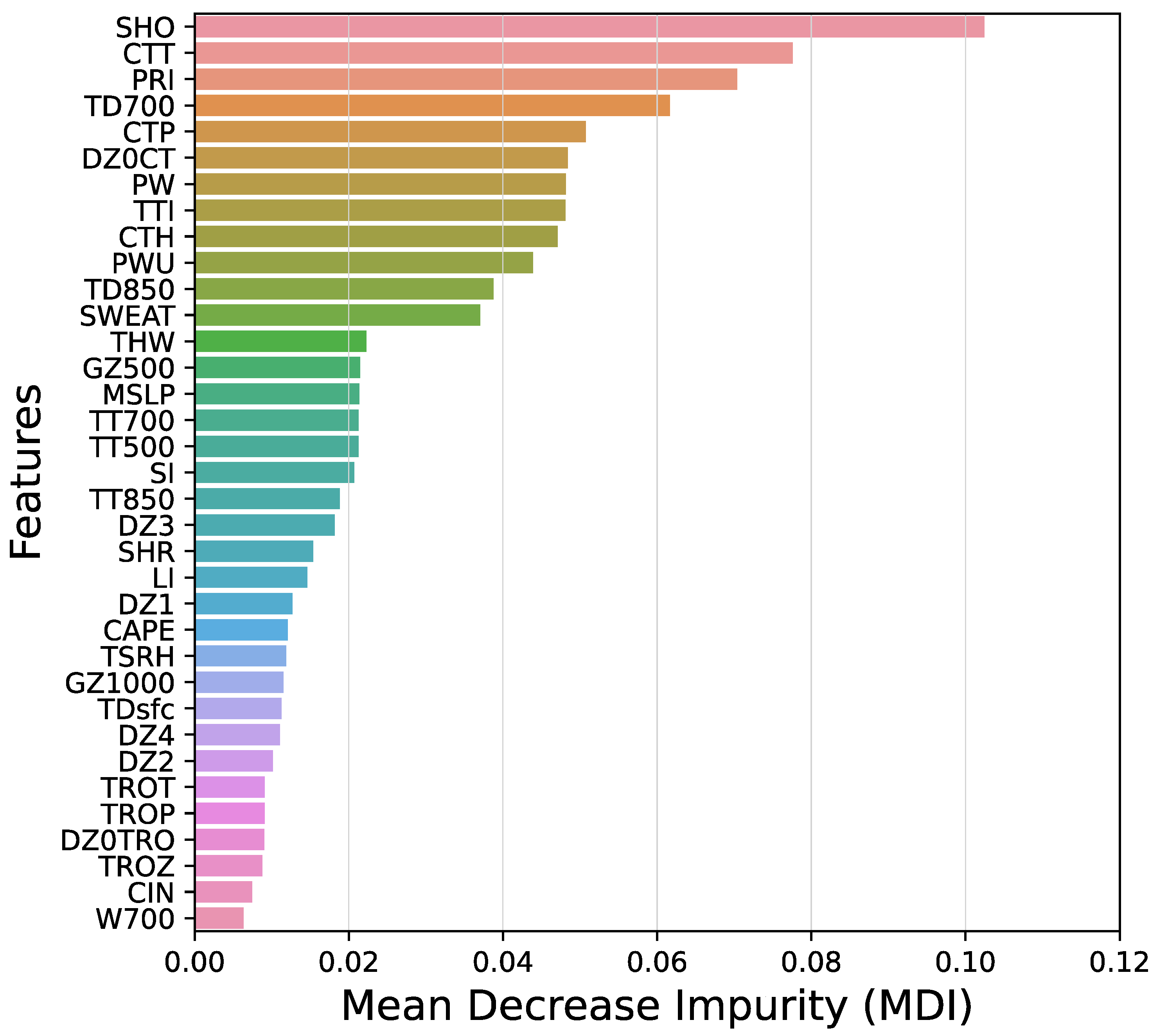
3.1. Feature Importance

The feature importance is measured by mean decrease impurity (MDI). MDI is one of the typical metrics used to assess the feature importance in tree-based methods. It is calculated by taking the mean and standard deviation of the impurity decrease within each tree. In other words, it measures how much each feature contributes to decreasing the impurity. If a particular feature significantly reduces impurity, it means that the feature plays a crucial role in classification. The feature importance in the trained model is shown in Figure 2.

The Showalter index (SHO) had the highest feature importance with a significantly high MDI (0.102). This suggested that SHO is the most important predictor for lightning occurrence prediction. This is consistent with a prior study that showed SHO had the highest importance for all trees [16]. Since lightning is typically accompanied by deep convection, it is believed that SHO, an instability index used for diagnosing atmospheric instability, had the highest importance.

The cloud-top-related variables (e.g., CTT (cloud top temperature), PRI, CTP, and CTH) exhibited high feature importance following SHO and were all ranked within the top 10. This can be attributed to the heightened utility of cloud-top-related variables in the KLAPS, which results from the assimilation of satellite data. However, the instability indices, including CAPE and LI, were ranked low, with CAPE at 22nd and LI at 24th. They are thought to have lower rankings compared to other instability indices, as they are not directly related to convection but rather associated with the possibility of convection.

3.2. Validation

The probabilistic prediction, given a value between 0 and 1, indicates the probability of the pixel belonging to lightning. The results of the deterministic prediction varied depending on the probability threshold. The default threshold was set at 50%, with probabilities above 50% predicting lightning (1) and those below 50% predicting non-lightning (0). We conducted deterministic predictions based on the threshold of probabilistic prediction and investigated the variations in skill scores.

Figure 3 illustrates the variations in skill scores for lightning with respect to the probability threshold for the stratified 10-fold cross-validation. The skill scores were derived by varying the threshold from 0 to 100 in increments of 0.01. As the threshold increased, the predicted lightning area diminished, leading to reductions in both POD and FAR, while precision increased. The CSI, which accounted for both POD and FAR, reached its peak value of 0.896 at a threshold of 46%. At this threshold, the precision was 0.940, the POD was 0.950, and the FAR was 0.060, demonstrating good performance.

These analyses enable users to choose a threshold for their purpose. If the aim is to reduce false alarms, a threshold with a low FAR should be used, whereas if the focus is on increasing hits, a threshold representing high POD or precision can be set for deterministic prediction.

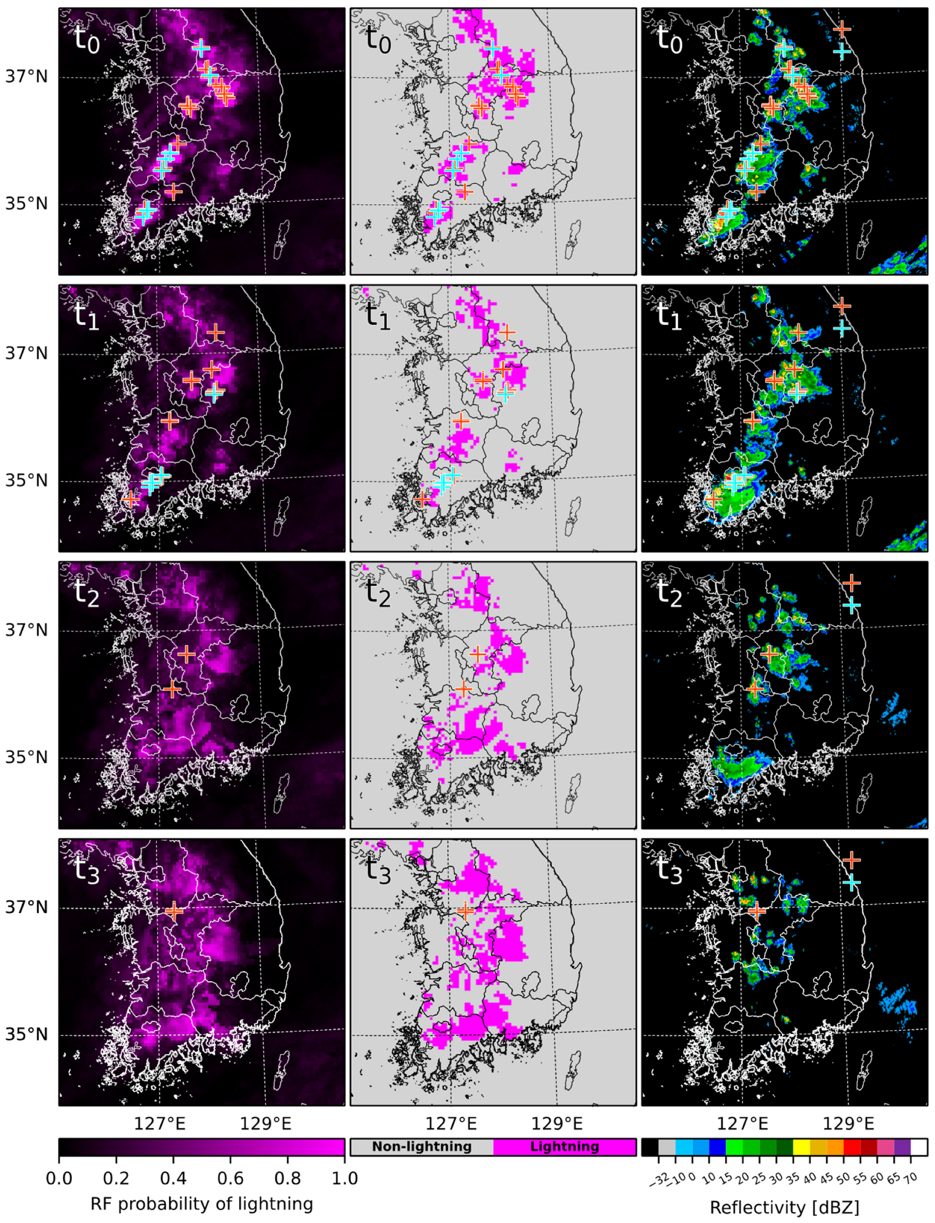
3.3. Application: Analysis and Forecast Field

We applied LightningRF to the entire grid of the KLAPS dataset to analyze the spatial distribution and investigate the potential of utilizing it for forecasting. LightningRF was trained using data from 2019 to 2021 and applied to the events in 2022.

The results of the probabilistic and deterministic prediction from LightningRF are displayed with the maximum radar reflectivity product (CMAX; column maximum radar reflectivity) (Figure 4, Figure 5 and Figure 6). The observed lightning is marked with a plus sign (orange: CG, cyan: CC), with the number of observations indicated in parentheses. In the deterministic prediction, lightning was predicted when the probability was equal to or greater than 0.46, which was the probability threshold with the highest CSI in the stratified 10-fold cross-validation. The lightning observation data consist of lightning events recorded within 10 min before the predicted time.

We manually selected three cases including squall line, convective systems, and widespread systems. LightningRF was utilized for the analysis field (${\mathrm{t}}_0$) and subsequently to forecast fields at 1-h intervals up to 3 h (${\mathrm{t}}_1$–${\mathrm{t}}_3$).

The first case shown in Figure 4 was a long north–south squall line that dissipated rapidly after 2 h of lead time. Comparing prediction and CMAX, LightningRF precisely predicted the movement of the precipitation system up to 1-h lead prediction. In particular, even in the 1-h lead forecast field, the model successfully captured the shape of the squall line with a high probability. With an increase in lead time, the probabilistic prediction area widened despite the structure of the squall line being broken.

In the late afternoon (1600 LST), small-scale convective cells were initiated on the windward side of the mountain (Figure 5). These cells were initially scattered but merged in the later time as they were developed. The LightningRF-predicted area of lightning occurrence generally agreed with the observations. Notably, the areas where lightning occurred were predicted with high probability. Specifically, for cloud-to-ground lightning, the average probabilities were 0.727, 0.523, 0.669, and 0.591 for ${\mathrm{t}}_0$, ${\mathrm{t}}_1$, ${\mathrm{t}}_2$, and ${\mathrm{t}}_3$, respectively. Additionally, the maximum probabilities for these times were 0.99, 0.945, 0.955, and 0.865, respectively. Despite being a convective cell in a small region where it is difficult to make predictions, it demonstrated the ability of the model to predict the lightning activity of convective cells.

Lastly, the third case was a widespread precipitation system extending across the Korean Peninsula (Figure 6). The region with a possibility of lightning occurrence was widely distributed, but the area with a high probability decreased over time. Contrary to convective cases, stratiform cases demonstrated a wider extent of forecast area for lightning. Furthermore, the implementation of a 46% probability threshold in deterministic predictions highlighted regions of lightning, even when the associated probabilities were relatively low.

Changes in the predicted probability at the location of lightning occurrence according to forecast lead time were investigated (Figure 7). We compared the results of LightningRF with a total of 41 h of forecast data from June to August 2022. To compare the observed lightning data, which consisted of point data, with the gridded predicted probabilities of lightning, the predicted probabilities were averaged over a 3 × 3 grid (i.e., 15 × 15 km²) centered on the observed lightning grid points. As anticipated, the probability of the event decreased as the prediction time increased. The probabilities for CG and CC exhibited a rapid decline during the first 2 h. However, after 3 h, the probabilities increased again, maintaining values above 0.5 for up to 7 h. Throughout the first 8 h, the probability of CC was predicted to be greater than that of CG, but this trend reversed sharply thereafter, resulting in a higher probability for CG. Consequently, it can be seen that RF-based lightning prediction can be effectively performed up to a lead time of 7 h.

4. Discussion

In this study, we developed the LightningRF model, which tends to overestimate the spatial extent of forecasted regions, resulting in increased false positive occurrences. Although we attempted to mitigate this issue by addressing data imbalance through undersampling, exploring more advanced methods for handling data imbalance could further alleviate overestimation. Additionally, while we selected a threshold of 46% for deterministic lightning prediction to maximize the CSI, increasing this threshold (e.g., to 70% or 80%) may reduce false alarms. This trade-off between the probability of detection and the false alarm ratio should be fine-tuned according to the specific application.

Our approach is largely dependent on the performance of the NWP model. If the NWP model inaccurately simulates the atmospheric conditions conducive to lightning, our model is likely to predict a high probability of lightning occurrence inaccurately. For this reason, it is crucial to continue improving NWP model performance while also enhancing observational studies to deepen our understanding of the relationship between lightning and other meteorological factors. In addition, future studies may benefit from incorporating high-resolution remote sensing data to enhance short-term predictions within the initial minutes to 1–2 h of forecast lead time. Potential data sources include radar reflectivity, vertically integrated liquid from radar, and satellite-obtained brightness temperatures [13].

An additional topic of interest is how lightning occurrence is defined. Defining the time interval for considering a lightning event is challenging given the instantaneous, point-based nature of lightning. Based on prior research and international standards [22,36,37,38], we defined a lightning event as any occurrence within 10 min before the predicted time. The selected temporal window might impact model performance: a longer window could compromise data representativeness, while a shorter window may result in overfitting. This presents an interesting opportunity for future exploration.

5. Conclusions

Lightning prediction is quite challenging as it develops rapidly and is confined to the spatial extent of convective storms. To provide accurate lightning prediction for forecasters and researchers, we proposed an RF model named LightningRF, based on high-resolution NWP analysis data (i.e., KLAPS). LightningRF was trained on thermodynamic and dynamic parameters derived from the KLAPS as predictors, with lightning observations provided by the KMA set as the response variable.

To address the issue of imbalanced data, we applied undersampling to construct the training dataset. The hyperparameters of the LightningRF model were optimized using a grid search approach combined with the stratified 10-fold cross-validation. The model was configured to use 200 trees, with four predictors randomly selected for each tree during the building process.

We conducted a feature importance analysis and found that the Showalter index acts as an important factor in lightning prediction. Following SHO, cloud top-related variables had high variable importance scores. On the other hand, instability indices such as CAPE, CIN, and LI were assigned comparatively lower rankings.

LightningRF was validated using the stratified 10-fold cross-validation. The skill scores for lightning prediction were investigated across various probability thresholds. When using the typical threshold of 50% or higher to predict lightning, both precision and POD exhibited good performance, exceeding 0.9. For deterministic prediction, we adopted a threshold of 46%, where CSI reached its peak.

We further applied LightningRF to both the KLAPS analysis field and the forecast fields. Probabilistic and deterministic predictions were conducted at each KLAPS grid point with high spatial resolution (grid spacing of 5 km). In convective cases, there was good agreement in predicting lightning occurrence areas, particularly up to a 1-h lead time. However, in stratiform cases, the predicted lightning areas were more broadly distributed. Analysis of the predicted probabilities for lightning occurrence areas with respect to forecast lead time revealed that LightningRF is applicable for forecasting up to a 7-h lead time.

References

1. Holle, R.L. A Summary of Recent National-Scale Lightning Fatality Studies. Weather Clim. Soc. 2016, 8, 35–42. [Google Scholar] [CrossRef]
2. Yair, Y. Lightning Hazards to Human Societies in a Changing Climate. Environ. Res. Lett. 2018, 13, 123002. [Google Scholar] [CrossRef]
3. Bright, D.R.; Wandishin, M.S.; Ryan, E.J.; Steven, J.W. A Physically Based Parameter for Lightning Prediction and Its Calibration in Ensemble Forecasts. In Proceedings of the 22nd Conference on Severe Local Storms, Hyannis, MA, USA, 3–8 October 2004; Available online: http://ams.confex.com/ams/pdfpapers/84173.pdf (accessed on 18 August 2024).
4. Showalter, A.K. A Stability Index for Thunderstorm Forecasting. Bull. Amer. Meteor. Soc. 1953, 34, 250–252. [Google Scholar] [CrossRef]
5. Bidner, A. The Air Force Global Weather Central Severe Weather Threat (SWEAT) Index—A Preliminary Report. In Air Weather Service Sciences Review; AWS: Seattle, WA, USA, 1970; pp. 2–5. [Google Scholar]
6. Price, C.; Rind, D. A Simple Lightning Parameterization for Calculating Global Lightning Distributions. J. Geophys. Res. 1992, 97, 9919–9933. [Google Scholar] [CrossRef]
7. Karagiannidis, A.; Lagouvardos, K.; Lykoudis, S.; Kotroni, V.; Giannaros, T.; Betz, H.-D. Modeling Lightning Density Using Cloud Top Parameters. Atmos. Res. 2019, 222, 163–171. [Google Scholar] [CrossRef]
8. Eom, H.-S.; Suh, M.-S. Analysis of Stability Indexes for Lightning by Using Upper Air Observation Data over South Korea. Atmosphere 2010, 20, 467–482. [Google Scholar]
9. Lecun, Y.; Bottou, L.; Bengio, Y.; Haffner, P. Gradient-Based Learning Applied to Document Recognition. Proc. IEEE 1998, 86, 2278–2324. [Google Scholar] [CrossRef]
10. Ronneberger, O.; Fischer, P.; Brox, T. U-Net: Convolutional Networks for Biomedical Image Segmentation. In Proceedings of the International Conference on Medical Image Computing and Computer-Assisted Intervention (MICCAI), Munich, Germany, 5–9 October 2015; pp. 234–241. [Google Scholar] [CrossRef]
11. Shi, X.; Chen, Z.; Wang, H.; Yeung, D.Y.; Wong, W.K.; Woo, W.C. Convolutional LSTM Network: A Machine Learning Approach for Precipitation Nowcasting. Adva. Neural Inf. Process. Syst. 2015, 28, 802–810. [Google Scholar] [CrossRef]
12. Zhou, K.; Zheng, Y.; Dong, W.; Wang, T. A Deep Learning Network for Cloud-to-Ground Lightning Nowcasting with Multisource Data. J. Atmos. Ocean. Technol. 2020, 37, 927–942. [Google Scholar] [CrossRef]
13. Li, Y.; Liu, Y.; Sun, R.; Guo, F.; Xu, X.; Xu, H. Convective Storm VIL and Lightning Nowcasting Using Satellite and Weather Radar Measurements Based on Multi-Task Learning Models. Adv. Atmos. Sci. 2023, 40, 887–899. [Google Scholar] [CrossRef]
14. Reynolds, S.E.; Brook, M.; Gourley, M.F. Thunderstorm Charge Separation. J. Meteor. 1957, 14, 426–436. [Google Scholar] [CrossRef]
15. Radhakrishna, B.; Zawadzki, I.; Fabry, F. Predictability of Precipitation from Continental Radar Images. Part V: Growth and Decay. J. Atmos. Sci. 2012, 69, 3336–3349. [Google Scholar] [CrossRef]
16. Burrows, W.R.; Price, C.; Wilson, L.J. Warm Season Lightning Probability Prediction for Canada and the Northern United States. Weather Forecast. 2005, 20, 971–988. [Google Scholar] [CrossRef]
17. Moon, S.-H.; Kim, Y.-H. Forecasting Lightning around the Korean Peninsula by Postprocessing ECMWF Data Using SVMs and Undersampling. Atmos. Res. 2020, 243, 105026. [Google Scholar] [CrossRef]
18. Breiman, L. Random Forests. Mach. Learn. 2001, 45, 5–32. [Google Scholar] [CrossRef]
19. Cortes, C.; Vapnik, V. Support Vector Networks. Mach. Learn. 1995, 20, 273–297. [Google Scholar] [CrossRef]
20. La Fata, A.; Amato, F.; Bernardi, M.; D’Andrea, M.; Procopio, R.; Fiori, E. Cloud-to-Ground Lightning Nowcasting Using Machine Learning. In Proceedings of the 2021 35th International Conference on Lightning Protection (ICLP) and XVI International Symposium on Lightning Protection (SIPDA), Colombo, Sri Lanka, 20 September 2021; pp. 1–6. [Google Scholar]
21. Geng, Y.; Li, Q.; Lin, T.; Yao, W.; Xu, L.; Zheng, D.; Zhou, X.; Zheng, L.; Lyu, W.; Zhang, Y. A Deep Learning Framework for Lightning Forecasting with Multi-source Spatiotemporal Data. Q. J. R. Meteorol. Soc. 2021, 147, 4048–4062. [Google Scholar] [CrossRef]
22. Leinonen, J.; Hamann, U.; Germann, U. Seamless Lightning Nowcasting with Recurrent-Convolutional Deep Learning. Artif. Intell. Earth Syst. 2022, 1, e220043. [Google Scholar] [CrossRef]
23. McGovern, A.; Lagerquist, R.; John Gagne, D.; Jergensen, G.E.; Elmore, K.L.; Homeyer, C.R.; Smith, T. Making the Black Box More Transparent: Understanding the Physical Implications of Machine Learning. Bull. Amer. Meteor. Soc. 2019, 100, 2175–2199. [Google Scholar] [CrossRef]
24. Brothers, M.D.; Hammer, C.L. Random Forest Approach for Improving Nonconvective High Wind Forecasting across Southeast Wyoming. Weather Forecast. 2023, 38, 47–67. [Google Scholar] [CrossRef]
25. Sandmæl, T.N.; Smith, B.R.; Reinhart, A.E.; Schick, I.M.; Ake, M.C.; Madden, J.G.; Steeves, R.B.; Williams, S.S.; Elmore, K.L.; Meyer, T.C. The Tornado Probability Algorithm: A Probabilistic Machine Learning Tornadic Circulation Detection Algorithm. Weather Forecast. 2023, 38, 445–466. [Google Scholar] [CrossRef]
26. Medina, B.L.; Carey, L.D.; Amiot, C.G.; Mecikalski, R.M.; Roeder, W.P.; McNamara, T.M.; Blakeslee, R.J. A Random Forest Method to Forecast Downbursts Based on Dual-Polarization Radar Signatures. Remote Sens. 2019, 11, 826. [Google Scholar] [CrossRef]
27. Shin, K.; Song, J.J.; Bang, W.; Lee, G. Quantitative Precipitation Estimates Using Machine Learning Approaches with Operational Dual-Polarization Radar Data. Remote Sens. 2021, 13, 694. [Google Scholar] [CrossRef]
28. Shin, K.; Kim, K.; Song, J.J.; Lee, G. Classification of Precipitation Types Based on Machine Learning Using Dual-Polarization Radar Measurements and Thermodynamic Fields. Remote Sens. 2022, 14, 3820. [Google Scholar] [CrossRef]
29. Pedregosa, F.; Varoquaux, G.; Gramfort, A.; Michel, V.; Thirion, B.; Grisel, O.; Blondel, M.; Prettenhofer, P.; Weiss, R.; Dubourg, V.; et al. Scikit-Learn: Machine Learning in Python. J. Mach. Learn. Res. 2011, 12, 2825–2830. [Google Scholar]
30. Lee, J.-C.; Lee, J.-S.; Lee, Y.H.; Lee, H.-C.; Chang, D.-E.; Lee, Y.H.; Lee, H.-C.; Chang, D.-E. Production of the high-resolution reanalysis data using KLAPS. In Proceedings of the Spring Meeting of KMS, Geryong, Republic of Korea, 29 April 2010; pp. 227–228. [Google Scholar]
31. Skamarock, W.C.; Klemp, J.B.; Dudhia, J.; Gill, D.O.; Barker, D.M.; Duda, M.G.; Huang, X.Y.; Wang, W.; Powers, J.G. NCAR Technical Note: A Description of the Advanced Research WRF Version 3; Mesoscale & Microscale Meteorology Division, National Center for Atmospheric Research: Boulder, CO, USA, 2008. [Google Scholar]
32. Livingston, E.S.; Nielsen-Gammon, J.W.; Orville, R.E. A Climatology, Synoptic Assessment, and Thermodynamic Evaluation for Cloud-to-Ground Lightning in Georgia: A Study for the 1996 Summer Olympics. Bull. Amer. Meteor. Soc. 1996, 77, 1483–1495. [Google Scholar] [CrossRef]
33. Kehrer, K.; Graf, B.; Roeder, W.P. Global Positioning System (GPS) Precipitable Water in Forecasting Lightning at Spaceport Canaveral. Weather Forecast. 2008, 23, 219–232. [Google Scholar] [CrossRef]
34. Kuk, B.-J.; Ha, J.-S.; Kim, H.-I.; Lee, H.-K. Statistical Characteristics of Ground Lightning Flashes over the Korean Peninsula Using Cloud-to-Ground Lightning Data from 2004–2008. Atmos. Res. 2010, 95, 123–135. [Google Scholar] [CrossRef]
35. Ukkonen, P.; Mäkelä, A. Evaluation of Machine Learning Classifiers for Predicting Deep Convection. J. Adv. Model. Earth Syst. 2019, 11, 1784–1802. [Google Scholar] [CrossRef]
36. European Union. Commission implementing regulation (EU) 2017/373 of 1 March 2017 laying down common requirements for providers of air traffic management/air navigation services and other air traffic management network functions and their oversight. Off. J. Eur. Union 2017, 60, L62. Available online: https://eur-lex.europa.eu/legal-content/EN/TXT/PDF/?uri=CELEX:32017R0373&from=EN (accessed on 23 September 2024).
37. International Civil Aviation Organization (ICAO). Annex 3 to the Convention on International Civil Aviation: Meteorological Service for International Air Navigation, 20th ed.; International Civil Aviation Organization: Montréal, QC, Canada, 2018; p. 250. [Google Scholar]
38. Mostajabi, A.; Finney, D.L.; Rubinstein, M.; Rachidi, F. Nowcasting Lightning Occurrence from Commonly Available Meteorological Parameters Using Machine Learning Techniques. NPJ Clim. Atmos. Sci. 2019, 2, 41. [Google Scholar] [CrossRef]
39. Turcotte, V.; Vigneux, D. Severe Thunderstorms and Hail Forecasting Using Derived Parameters from Standard RAOBS Data. In Proceedings of the Second Workshop on Operational Meteorology, Halifax, NS, Canada, 14–16 October 1987; pp. 142–153. [Google Scholar]
Figure 1. Locations of lightning sensors (red dot) over the Korean peninsula.
Remotesensing 16 03621 g001
Figure 2. The importance of the features (mean decrease impurity), ranked in descending order from top to bottom. Greater mean decrease impurity reflects higher variable importance.
Remotesensing 16 03621 g002
Figure 3. Skill scores from stratified 10-fold cross-validation for lightning as a function of a probability threshold. The colors indicate each skill score: precision (red), POD (green), FAR (blue), and CSI (black). The black dot represents the maximum value of CSI.
Remotesensing 16 03621 g003
Figure 4. Probabilistic prediction (left) and deterministic prediction (i.e., probability ≥ 0.46) of lightning from the RF (center), and CMAX (right) at 0700 UTC on 11 June 2022 from the current time ( t 0 ) to 3-h lead prediction ( t 3 ) at a 1-h interval. Lightning observations are indicated by a plus sign at each timestep, with orange denoting cloud-to-ground lightning and cyan denoting cloud-to-cloud.
Remotesensing 16 03621 g004
Figure 5. Same as Figure 4, but at 0700 UTC on 3 July 2022.
Remotesensing 16 03621 g005
Figure 6. Same as Figure 4, but at 0500 UTC on 13 August 2022.
Remotesensing 16 03621 g006
Figure 7. The predicted probability at the location of observed lightning as a function of forecast lead time.
Remotesensing 16 03621 g007
Disclaimer/Publisher’s Note: The statements, opinions and data contained in all publications are solely those of the individual author(s) and contributor(s) and not of MDPI and/or the editor(s). MDPI and/or the editor(s) disclaim responsibility for any injury to people or property resulting from any ideas, methods, instructions or products referred to in the content.