Abstract
Hyperspectral small target detection (HSTD) is a promising pixel-level detection task. However, due to the low contrast and imbalanced number between the target and the background spatially and the high dimensions spectrally, it is a challenging one. To address these issues, this work proposes a representation-learning-based graph and generative network for hyperspectral small target detection. The model builds a fusion network through frequency representation for HSTD, where the novel architecture incorporates irregular topological data and spatial–spectral features to improve its representation ability. Firstly, a Graph Convolutional Network (GCN) module better models the non-local topological relationship between samples to represent the hyperspectral scene’s underlying data structure. The mini-batch-training pattern of the GCN decreases the high computational cost of building an adjacency matrix for high-dimensional data sets. In parallel, the generative model enhances the differentiation reconstruction and the deep feature representation ability with respect to the target spectral signature. Finally, a fusion module compensates for the extracted different types of HS features and integrates their complementary merits for hyperspectral data interpretation while increasing the detection and background suppression capabilities. The performance of the proposed approach is evaluated using the average scores of , , , and . The corresponding values are 0.99660, 0.00078, 0.99587, and 333.629, respectively. These results demonstrate the accuracy of the model in different evaluation metrics, with achieving the highest score, indicating strong detection performance across varying thresholds. Experiments on different hyperspectral data sets demonstrate the advantages of the proposed architecture.
1. Introduction
Hyperspectral images (HSIs) are widely applied in land cover mapping, agriculture, urban planning, and other applications [1]. The high spectral resolution of HSIs enables the detection of a wide range of small and specific targets through spatial analysis or visual inspection [2]. Hyperspectral imaging offers numerous advantages for target detection, especially in high-precision and sensitive applications. By capturing detailed spectral information through hundreds or thousands of narrow bands, it distinguishes subtle differences between materials like minerals, vegetation, and chemicals. Even with mixed pixels, spectral unmixing can identify small or blended targets. Compared to traditional imaging methods, hyperspectral imaging provides greater accuracy and robustness, especially in complex backgrounds, while reducing false detections. It is highly useful for applications like environmental monitoring, military surveillance, agriculture, and food quality control. The technology allows for remote, real-time data collection, making it versatile and valuable across multiple fields.
In HSIs, the definition of small targets typically depends on the specific application scenario and task requirements. For instance, if the task is to detect traffic signs in HSIs, small targets may be defined as objects with traffic sign characteristics, with their size determined by the actual dimensions of traffic signs. These small targets usually have dimensions ranging from the pixel level to a few dozen pixels. Although their size may be minuscule compared to the entire image, they hold significant importance in specific contexts. Additionally, the semantic content of small targets may carry particular significance; for example, HSIs may include various objects such as vehicles, buildings, and people.
In this topical area, the most challenging targets in HSIs have the following characteristics. (1) Weak contrast: HSIs with their high spectral resolution but lower spatial resolution depict spatially and spectrally complex scenes, affected by sensor noise and material mixing; the targets are immersed in this context, leading to usually weak contrast and low signal-to-noise ratio (SNR) values. (2) Limited numbers: Due to the coarse spatial resolution, a target often occupies only one or a few pixels in a scene, which provides limited training samples. (3) Spectral complexity: HSI contains abundant spectral information. This leads to a very large dimension of the feature space, strong data correlation in different bands, extensive data redundancy, and eventually long computational times. In HSTD, the background typically refers to the parts of the image that do not contain the target. Compared to the target, the background usually has a higher similarity in color, texture, or spectral characteristics with the surrounding area, resulting in lower contrast within the image. This means it does not display distinct characteristics or significant differences from the surrounding regions. Background areas generally exhibit a certain level of consistency, with neighboring pixels having high similarity in their attributes. For example, a green grass field, a blue sky, or a gray building wall. This consistency means that the background may show relatively uniform spectral characteristics. Additionally, the background usually occupies a larger portion of the image and may have characteristics related to the environment, such as terrain, vegetation types, and building structures. These characteristics help distinguish the background from the target area. Accurately defining and modeling the background is crucial for improving the accuracy and robustness of target detection.
Based on these characteristics, the algorithms for HSI target extraction may be roughly subdivided into two big families: more traditional signal detection methods and more recent data-driven pattern recognition and machine learning methods.
Traditionally, detection involves transforming the spectral characteristics of target and background pixels into a specific feature space based on predefined criteria [3]. Targets and backgrounds occupy distinct positions within this space, allowing targets to be extracted using threshold or clustering techniques. In this research domain, diverse descriptions of background models have led to the development of various mathematical models [4,5,6,7] for characterizing spectral pixel changes.
The first category of algorithms in this family are the spectral-information-based models when the target and background spectral signatures are supposed to be generated by a linear combination of end member spectra. The Orthogonal Subspace Projection (OSP) [8] and the Adaptive Subspace Detector (ASD) [9] are two representative subspace-based target detection algorithms. OSP employs a signal detection method to remove background features by projecting each pixel’s spectral vector onto a subspace. However, the fact that the same object may have distinct spectra and the same spectra may appear in different objects because of spectral variation caused by the atmosphere, sensor noise, and the mixing of multiple spectra makes the identification of a target more challenging in reality due to imaging technology limitations [10]. To tackle this issue, Chen et al. proposed an adaptive target pixel selection approach based on spectral similarity and spatial relationship characteristics [11], which addresses the pixel selection problem.
A second category consists of statistical methods. These approaches assume that the background follows a specified distribution and then establish whether or not the target exists by looking for outliers with respect to this distribution. The Adaptive Cosine consistency Estimator (ACE) [12] and the Adaptive Matched Filter (AMF) [13] are among the techniques in this group, both of which are based on the Generalized Likelihood Ratio-based detection Test (GLRT) method [14].
Both ACE and AMF are spectral detectors that measure the distance between target features and data samples. ACE can be considered as a special case of a spectral angle-based detector. AMF was designed based on the hypothesis testing method for Gaussian distributions. The third category comprises representation-based methods that do not assume any data distribution, e.g., Constrained Energy Minimization (CEM) [15,16], hierarchical CEM (hCEM) [17], ensemble-based CEM (eCEM) [18], sCEM [19], target-constrained inference-minimized filter (TCIMF), and sparse representation (ST)-based methods [20]. Among these approaches, the classic and foundational CEM method constrains targets while minimizing the variance of data samples, and the TCIMF method combines CEM and OSP.
The most recent deep learning methods for target detection are mainly based on data representations involving kernels, sparse representations, manifold learning, and unsupervised learning. Specifically, methods based on sparse representation take into account the connections between samples in the sparse representation space. The Combined Sparse and Collaborative Representation (CSCR) [21] and the Dual Sparsity Constrained (DSC) [22] methods are examples of sparse representation. However, the requirement for exact pixel-wise labeling makes the task of achieving good performance an expensive one. To address the challenge of obtaining pixel-level accurate labels, Jiao et al. proposed a semantic multiple-instance neural network with contrastive and sparse attention fusion [23]. Kernel-based transformations [24] are employed to address the linear inseparability issue between targets and background in the original feature space. Gaussian radial basic kernel functions are commonly used, but there is still a lack of rules for choosing the best-performing kernel. Furthermore, in [25], manifold learning is employed to learn a subspace that encodes discriminative information. Finally, for unsupervised learning methods, an effective feature extraction method based on unsupervised networks is proposed to mine intrinsic properties underlying HSIs. The spectral regularization is imposed on autoencoder (AE) and variational AE (VAE) to emphasize spectral consistency [26]. Another novel network block with the region-of-interest feature transformation and the multi-scale spectral-attention module is also proposed to reduce the spatial and spectral redundancies simultaneously and provide strong discrimination [27].
While recent advancements have shown increased effectiveness, challenges remain in efficiently tuning a large number of hyperparameters and obtaining accurate labels [28,29]. Moreover, the statistical features extracted by GAN-based methods often overlook the potential topological structure information. Such a phenomenon greatly limits the ability to capture non-local topological relationships to better represent the underlying data structure of HSI. Thus, the representative features are not fully exploited and utilized to preserve the most valuable information across different networks. Detecting the location and shape of small targets with weak contrast against the background remains a significant challenge. Therefore, this paper proposes a deep representative model of the graph and generative learning fusion network with frequency representation. The goal is to develop a stable and robust model based on an effective feature representation. The primary contributions of this study are summarized as follows:
- We explore a collaboration framework for HSTD with less computation cost and high accuracy. Under the framework, the feature extraction from the graph and generative learning compensate for each other. To our knowledge, it is the first work to explore the collaborative relationship between the graph and generative learning in HSTD.
- The graph learning module is established for HSTD. The GCN module aims to compensate for the information loss of details caused by the encoder and decoder via aggregating features from multiple adjacent levels. As a result, the detailed features of small targets can be propagated to the deeper layers of the network.
- The primary mini batch GCN branch for HSTD is designed by following an explicit design principle derived from the graph method to reduce high computational costs. It enables the graph to enhance the feature and suppress noise, effectively dealing with background interference and retaining the target details.
- A spectral-constrained filter is used to retain the different frequency components. Frequency learning is introduced into data preparation for coarse candidate sample selection, favoring strong relevance among pixels of the same object.
2. Graph Learning
A graph describes one-to-many relations in a non-Euclidean space [30], and includes directed and un-directed patterns. It can be combined with a neural network to design Graph Convolution Networks (GCNs), Graph Attention Networks (GATs), Graph Autoencoders (GAEs), Graph Generative Networks (GGNs), and Graph Spatial-Temporal Networks (GSTNs) [31].
Among the graph-based networks mentioned above, this work focuses on GCNs, a set of neural networks that infer convolution from traditional data to graph data. Specifically, the convolution operation can be applied within a graph structure, where the key operation involves learning a mapping function. In this work, an undirected graph models the relationship between spectral features and performs feature extraction [32]. In matrix form, the layer-wise propagation rule of the multi-layer GCN is defined as
where denotes the output at the -th layer. is the activation function with respect to the weights to be learned and the biases of all layers. Drepresents a diagonal matrix of node degrees. represents the adjacency matrix of undirected graph G added to the identity matrix of proper size throughout this article.
Deep-learning-based approaches to HSIs based on graph learning are increasingly common, especially for detection and classification. For instance, Weighted Feature fusion of Convolutional neural network and Graph attention network (WFCG) exploits the complementary characteristics of superpixel-based GAT and pixel-based CNN [33,34]. Additionally, a Robust Self-Ensembling Network (RSEN) has been proposed, comprising a base and ensemble network, which achieves satisfactory results even with limited sample sizes [35].
3. Proposed Methodology
3.1. Overall Framework
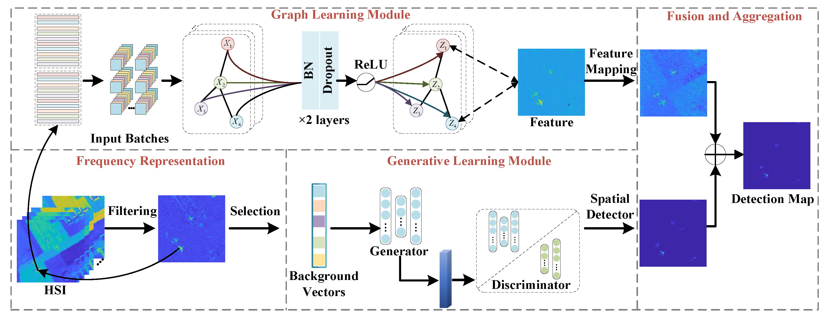
This section proposes a graph and generative learning network with frequency representation. The architecture of this method is shown in Figure 1 and consists of the GCN and GAN modules, to represent different types of features, with frequency learning assisting in selecting the initial pseudo labels. The graph learning module’s structure defines topological interactions in small batches to minimize computational resource requirements and refine the spatial features from HSI. The goal is to obtain spatially and spectrally representative information from both latent and reconstructed domains. This information is based on components extracted in the generative learning module to leverage the discriminative capacity of GAN models. A fusion module then exploits the association between these two complementary modules.

Figure 1.
Graphical representation of the flowchart of the proposed method, comprising four major modules: (1) a graph learning module, (2) a generative learning module, (3) a frequency representation module, and (4) a fusion module. The first module extracts the underlying data properties from the original HSI, while the second provides complementary spectral and spatial characteristics. The frequency learning module is added before training to achieve the frequency representation of the component by analyzing the spectral properties of HSIs to extract relevant features. Finally, the fusion module integrates the two modules to achieve more comprehensive feature extraction and information aggregation.
The description of the problem formulation is as follows. Let us denote the HSI by , where M, N, C are the three dimensions of the image. The input HSI consists of the background set and target set , i.e., , and , . According to these definitions, the establishment of the overall model is given by
where is the output of the GCN function . is the Laplacian matrix. is the output of GAN. and are the input to the testing and the training phase, respectively. is the coefficient setting the percentage of the training samples .
3.2. Data Preparation Based on Frequency Learning
Prior to any detection step, the first step of the processing chain is a subdivision of the original HSI into frequency representation components. For images, frequency learning can be used to enhance features, reduce noise, and compress data by focusing on the significant frequency components. We analyze the spectral properties of images to extract relevant features. The filter output is the input to the upper and lower branches of the architecture in Figure 1. The idea is that the high-frequency component plays a significant role in depicting smaller targets. Some specific information in high-frequency components, such as object boundaries, can more effectively distinguish different objects. Unlike natural images, HSI contains rich spectral and spatial information. The low-frequency component refers to its continuous smooth part in the spatial domain, which indicates the similarity of spectral features between adjacent pixels. Additionally, in the case of original labels, low-frequency components are more generalizable than high-frequency components, which may play an essential role in detecting particular smaller objects. Therefore, detecting objects in the frequency domain may be more suitable for small and sparse hyperspectral targets [36,37].
Based on the above ideas, this work passes the original HSI through a designed linear FIR filter to obtain a pseudo-label map through CEM-inspired algorithm. The filtered signal includes high-frequency components from the image with significant gradients, representing edges. Also, it includes low-frequency components in the image with relatively slow frequency changes. Combining high- and low-frequency components, each representing distinct physical characteristics, as inputs to the network, enhances the accuracy of target detection. The filter output serves as input to both the upper and lower branches of the architecture in Figure 1. For the GCN module, graph structure convolution is analogous to a Fourier transform that defines the original frequency signal. The combination of frequency components obtained by filtering is subjected to Fourier transform in the frequency domain to realize spectral-domain graph convolution. The input of GCN includes pixel-level samples and an adjacency matrix that models the relationship between samples.
Specifically, the filter’s design is about the hCEM-inspired function. The traditional CEM algorithm designs a filter such that the energy of the target signal remains constant after passing through it, thereby minimizing total output energy under these conditions. However, the detection effect of this filter may not be achieved through one single layer. Therefore, the hCEM algorithm [17] connects multiple layers of CEM detectors in series and uses a nonlinear function to suppress the background spectrum. Each CEM layer processes the spectrum as input for the subsequent layer, progressively enhancing the detector’s effectiveness. The filter designed in this way helps in identifying the target. With a similar idea, frequency filtering in this work is
where represents the filter function. The latent variable, denoted as , is obtained by the following steps. First, the HSI and prior target spectral signature are put in as input to the initial network. Then, white Gaussian noise is added to each spectral vector, and the latent variable is computed. Calculation stops once the output converges to a constant , where the initial value of is the spectral vector of the , and represents the number of spectral vectors.
The filter coefficient is designed to suppress the background spectrum as
where d represents a prior spectral vector.
The output of the m-th layer is
and the stopping condition is defined as
In each iteration, the previous output is utilized in the training phase. Iterations conclude when the stopping condition is met, yielding a final output .
Values in sort the pixels based on filtering results: values closer to 0 indicate higher probability of background, while values closer to 1 suggest a higher likelihood of being a target. Solely relying on low frequencies limits discriminative ability in frequency learning [38]. This is because node representations become similar by only aggregating low-frequency signals from neighbors, regardless of whether the nodes belong to the same class. Therefore, for GAN, the pseudo-target, and the pseudo-background vectors are input into the network simultaneously; the network learns high-frequency and low-frequency parts. The proposed network integrates the benefits from both low-frequency and high-frequency signal representations. The output from this frequency learning module serves as input for training and testing phases, with detailed process and network structure descriptions as follows.
3.3. The Graph Learning Module
This section introduces the graph learning module. The output from the frequency learning module serves as input for both the training and testing phases, accompanied by a detailed process and network structure description.
Due to the ability to represent the relations between samples, effectively handle graph structure data, and be compatible with HSIs, a GCN is the perfect fit as the basic structure [33]. The traditional discrete convolution of CNN cannot maintain translation invariance on the data of a non-Euclidean structure. Due to varying adjacency in the topology graph, convolution operations cannot use kernels of uniform size for each vertex’s adjacent vertices. CNN cannot handle the data of non-Euclidean structures, but it is expected to effectively extract spatial features on such a topological structure [39]. And GCN is employed as an undirected graph to represent the relations between spectral signatures in the proposed method. When building the model, the network is supposed to effectively characterize the non-structural feature information between different spectral samples and complement the representation ability of the traditional spatial–spectral joint features obtained by CNNs. Therefore, it aims to build the GCN to achieve multiple updates in each epoch. In traditional GCNs, pixel-level samples are fed into the network through an adjacency matrix that models the relationship among samples and that must be computed before the training begins. However, the huge computational cost caused by the high dimensionality of HSIs limits graph learning performances for these data. This is why this work’s local optimum training in a mini-batch pattern (similar to CNN) was adopted. The mini-batch decreases the high computational cost of constructing an adjacency matrix on high-dimensional data sets and improves binary detection training and model convergence speed. In [40], it is theoretically applicable in using mini-batch training strategies.
Figure 1 illustrates the GCN structure within the proposed target detection framework. Here, denotes an undirected graph with vertex set V and edge set E. HS pixels define vertex sets, with similarities establishing the edge set. Adjacency matrix construction and spectral domain convolution proceed as follows.
The adjacency matrix defines the relationship between vertexes. Each element in can generally be computed by , where is a parameter to control the width of the Radial Basis Function (RBF) included in the formula. The vectors and denote the spectral signatures associated with the vertexes and . Given , the corresponding graph Laplacian matrix may be computed as , in which is a diagonal matrix representing the degrees of , i.e., . Describing graph convolution involves initially extracting a set of basis functions by computing eigenvectors of . Then, the spectral decomposition of is performed according to
The convolution between f and g on a graph with coefficient can thus be expressed as
Accordingly, the propagation rule for GCN can be represented as
where and are the re-normalization terms of and , respectively, used to enhance the stability in the process of the network training. Additionally, represents the layer’s output, with serving as the activation function in the final layer (e.g., ReLU).
The unbiased estimator of the node in the full batch GCN layer, denoted as
where s is not only the s-th sub-graph but also the s-th batch in the network training.
Dropout is applied to the first GCN layer to prevent overfitting, thereby preventing all pixels from being misdetected as background during training.
3.4. Generative Learning Module
The GCN focuses on global feature smoothing by aggregating intra-class information and making intra-class features similar. Complementarily, a generative learning module was introduced into the model to enhance the distinction between the two classes. During the training phase, the generator is pre-trained on pseudo samples. Consequently, it could be regarded as a function that transforms noise vector samples from the d-dimensional latent space to pixel-space-generated images.
The generator G minimizes and generates output samples of the encoder to match the distribution of , deceiving discriminator D. The network’s output can be described as follows:
where is the extracted feature of the encoder. are the weights and biases of the encoder and decoder.
When training converges, the discriminator fails to distinguish between generated and target data. serves as the testing and detection network in the generative module, obtaining maps from trained parameters.
3.5. Fusion and Aggregation Module
Extracting statistical features from data often overlooks the potential topological structure information between different land cover categories. GAN-based methods typically only model the local spatial relationships of samples, which greatly limits the ability to capture non-local topological relationships, better representing the underlying data structure of HSIs. To alleviate this issue, in this work, the deep representative model fuses different modules and enhances the feature discrimination ability by combining the advantages of the graph and generative learning. Specifically, the proposed GCNs can be combined with standard GAN models as follows:
where is the detection map of the whole network. and are the output of generative and graph learning modules, respectively. represents the nonlinear aggregation module. The feature mapping function transforms extracted features through GCN into detection maps, effectively suppressing background.
The outputs from the graph convolution module and generative training module can be considered as features. Since the generative model is able to extract spatial–spectral features and graph learning represents topological relations between samples, combining both models should provide better results exploiting feature diversity. The nonlinear processing after two modules provides a more robust nonlinear representation ability of the features; aggregates the small targets, which are hard to detect; and suppresses the complex background similar to the targets.
4. Experimental Results and Analysis
4.1. Data Sets
The performance of the proposed approach and state-of-the-art techniques were evaluated on five data sets, including the HYDICE, San Diego, ABU−1 (Texas Coast-1), ABU−2 (Texas Coast-2), and ABU−3 (Los Angeles) data sets. The details of the data sets are shown in Table 1.

Table 1.
Descriptions of the data sets.
4.1.1. HYDICE Data Set
The first data set was recorded by the hyperspectral digital imagery collection experiment (HYDICE) sensor (http://www.erdc.usace.army.mil/Media/FactSheets/FactSheetsArticleView/tabid/9254/Article/476681/hypercube, accessed on 23 September 2024). It contains 162 bands after removing the noisy bands in a total of 210 bands with a sub-image of 80 × 100 for each band. Figure 2a shows the pseudo-color image and ground truth.
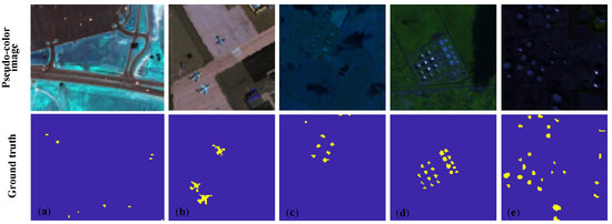
Figure 2.
The pseudo-color image and ground-truth for (a) HYDICE, (b) San Diego, (c) ABU−1, (d) ABU−2, (e) ABU−3.
4.1.2. San Diego Data Set
The second data set was captured by the Airborne Visible/Infrared Imaging Spectrometer (AVIRIS) sensor (http://aviris.jpl.nasa.gov/, accessed on 16 November 2011). It is accessed on 16 November 2011. After the water vapor absorption and low SNR bands are removed, the sub-image is sliced from the original scene at the center of the original scene. The background contains hangars, parking aprons, and exposed soil. Figure 2b shows the pseudo-color image and ground truth.
4.1.3. Texas Coast Data Set
The third and fourth data sets were acquired by the AVIRIS sensor. They were obtained from Airport–Beach–Urban (ABU) data sets with a series of scenes of the Texas Coast (http://xudongkang.weebly.com/, accessed on 29 August 2010). Noisy bands in the original images have been removed. The first scene contains 100 × 100 pixels in the spatial domain with 204 bands. The second scene contains 100 × 100 pixels in the spatial domain with 207 bands. Figure 2c,d show the pseudo-color image and ground truth.
4.1.4. Los Angeles Data Set
The fifth data set was also from ABU data sets and was captured by the AVIRIS sensor covering the Los Angeles city area with noisy bands in the original images (http://xudongkang.weebly.com/, accessed on 11 September 2011). It contains 100 × 100 pixels in the spatial domain with 205 bands. Figure 2e shows the pseudo-color image and ground truth.
Bold indicates the best value under the metric, and underline indicates the second-best value under the metric.
4.2. Evaluation Indexes
Several metrics, i.e., the receiver operating characteristic (ROC) and the area under the curve (AUC), were leveraged for performance evaluation. Specifically, the 3D ROC curve of , , and was used to evaluate the detector effectiveness and the background suppression ability [2,41]. The is a measure that is obtained by subtracting from to describe the background suppression ability. The is a measure that is obtained by dividing by . It describes the signal-to-noise rate of the methods, where the false alarm probability can be assumed to be caused by noise. When the value is higher, the performance of the detector is better.
4.3. Implementation Details
Prior spectra in HSTD can be obtained by laboratory measurements or simulations. In this experiment, we obtain it by calculating the mean of the target spectra according to the ground truth. Compared to the commonly used optimization methods, such as Adagrad and Momentum optimization, the Adam algorithm is chosen for optimization with a better performance. The learning rate is set to 0.0001 and updated every 50 epochs. The normalization adopts batch normalization, and the momentum is set to 0.9. The mini-batch is a set amount of training samples that are less than the total training samples in the data set. In each iteration, the batch size of the network on a different set of samples is set to 32 until all of the samples are used in the data set. As the number of layers increases, the model does not show a noticeable accuracy increase because an over-deep network leads to over-smoothing, thus leading to poor training accuracy. Accordingly, this work sets the depth to two layers: a balance of complexity and performance. For graph learning, the module converges when the interaction is 200. For the generative module, the training model parameters and checkpoint are saved every 200 iterations, and the number of cycles is adaptively determined in the test phase according to the detection accuracy.
4.4. Comparison Methods
For comparison, eight state-of-the-art methods were selected, i.e., CEM [6], ACE [12], hCEM [17], eCEM [18], CSCR [21], DSC [22], BLTSC [28], and WHTD [29]. All these methods were re-implemented according to the papers and open-source code. The AUC scores are listed in Table 2, Table 3, Table 4, Table 5 and Table 6. According to them, the performance of the proposed model is superior to the compared methods in the and . The target detection and background suppression ability outperform other methods on most data sets.

Table 2.
The quantitative results of the compared and proposed methods on the San Diego Data Set.

Table 3.
The quantitative results of the compared and proposed methods on the ABU−2 Data Set.

Table 4.
The quantitative results of the compared and proposed methods on the ABU−3 Data Set.

Table 5.
The quantitative results of the compared and proposed methods on the ABU−1 Data Set.

Table 6.
The quantitative results of the compared and proposed methods on the HYDICE Data Set.
4.5. Analysis of the Results
This section presents quantitative and qualitative experiments to validate the effectiveness of the proposed method. Performance evaluation includes 2D detection maps, 3D detection maps, 3D ROC analysis, and box-plot analysis, detailed as follows.
4.5.1. Quantitative Analysis
Table 2, Table 3, Table 4, Table 5, Table 6 and Table 7 show the assessment of different methods for different data sets through six different evaluation indexes.

Table 7.
Average scores of , , , and for the compared methods on different data sets.
For the HYDICE Data Set, although the proposed method has slightly lower detection accuracy than hCEM, its false alarm rate is one order of magnitude better than the other methods, resulting in better and . So as on ABU-2 data set, the performance of the proposed method is comparable in , , and , which is mainly due to the different compensatory representation of the fusion network. For the San Diego Data Set, the of the proposed method reaches 0.99362, and the of the proposed is 0.993, which is better than the others. For ABU-2 and ABU-3 Data Sets, the proposed method performs well on most indexes, proving the effectiveness of graph and generative learning modules with frequency representation.
The proposed method gives better results for some metrics and not others due to trade-offs in detecting targets. For example, improving precision might reduce recall, or handling noise better could lower sensitivity in detecting smaller or mixed targets. Different metrics measure various aspects like accuracy, robustness, and false positives, so excelling in one may lead to compromises in others depending on the method’s strengths and focus.
The selection of datasets is critical for hyperspectral target detection algorithms, as it affects accuracy, generalization, and adaptability. Higher spectral resolution improves material distinction but may introduce noise and data redundancy, while higher spatial resolution allows more precise target identification but can cause mixed pixel issues. Diverse datasets help algorithms generalize better to new environments, while high-quality and precise annotations improve detection accuracy, especially in complex scenarios. Hyperspectral data often contain noise, and algorithms must be robust enough to handle it. A well-chosen dataset with strong resolution, diversity, and representativeness significantly enhances algorithm performance, making it a key factor in development and testing.
To provide a comprehensive performance comparison of the proposed algorithm, Table 7 calculates the average scores for five real scene hyperspectral datasets, evaluating each method’s performance.
The measurement indicates the false alarm rate of the proposed method. However, when accuracy reaches a high level, the false alarm rate will increase to some extent. Thus, it is difficult to achieve good results for both for all the indexes. For certain application scenes, the high accuracy rather than low false alarm rate is required; therefore, designing an algorithm with high accuracy is important. The proposed algorithm reaches the optimum on the average of , , , and , which demonstrates better detection and background suppression ability.
4.5.2. Visual Analysis
Figure 3 depicts the detection results of several approaches on diverse data sets. The targets and certain partial regions around the targets are highlighted.
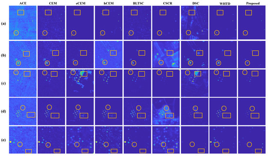
Figure 3.
The visual detection results of different detectors for the (a) HYDICE. (b) San Diego. (c) ABU−1. (d) ABU−2. (e) ABU−3. The targets and certain partial regions around the targets are highlighted through circle and box, respectively.
For HYDICE Data Sets, as shown in Figure 3a, the hCEM effectively decreases uniform background interference. However, there is blatant background noise interference around the target. Although there is some misdetection without background suppression and unstable performance in the CEM and CSCR methods, the recognition of structure and location is better. Despite some noise points in the background leading to occasional misidentifications in DSC, the method precisely locates targets. BLTSC rarely mistakes background for targets due to its background learning and spectral constraints. The WHTD method, employing weakly supervised background estimation with target-based constraints and channel-wise attention, achieves clear and accurate target detection. The proposed method effectively detects targets and suppresses background, leveraging non-local and spectral-spatial information representation through the commentary architecture.
For the San Diego Data Set, depicted in Figure 3b, eCEM and hCEM methods struggle with spectral variations in real scenes. The proposed detection map exhibits more precise and accurate target shapes, closely resembling ground truth as seen in BLTSC.
In the ABU−1 Data Set in Figure 3c, the proposed method achieves greater precision in target shape, with results closer to ground truth, featuring improved edge detection and smaller target recognition.
For the ABU−2 Data Set in Figure 3d, the proposed method focuses on accurate target detection while suppressing background interference. ACE and CEM methods identify fewer target pixels but demonstrate superior performance.
In Figure 3e, hCEM and DSC efficiently detect small targets in the ABU−3 Data Set. The proposed method shows slightly blurred edges in the detected targets but effectively suppresses the background. The q uantitative results align with findings from the 2D detection map.
The corresponding 3D views of the detection results are depicted in Figure 4, demonstrating the background and target values and the discrimination visualization. The 2D and 3D results show that the proposed method performs better with more precise targets and lower background values in background suppression. This is mainly due to the compensation of both the GAN and GCN in feature extraction and representation ability to the detection. The hCEM, CSCR, and proposed method for the LA data set could maintain target morphology while attaining high detection values at target pixels.
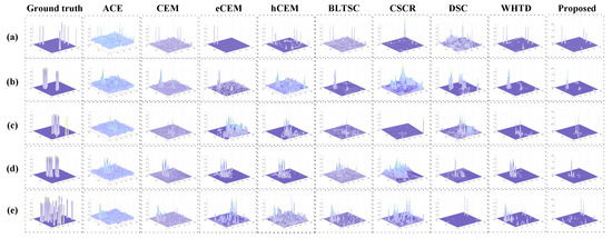
Figure 4.
The 3D detection maps of different detectors for the (a) HYDICE (b) San Diego (c) ABU−1 (d) ABU−2 and (e) ABU−3.
4.5.3. Three-Dimensional ROC Analysis
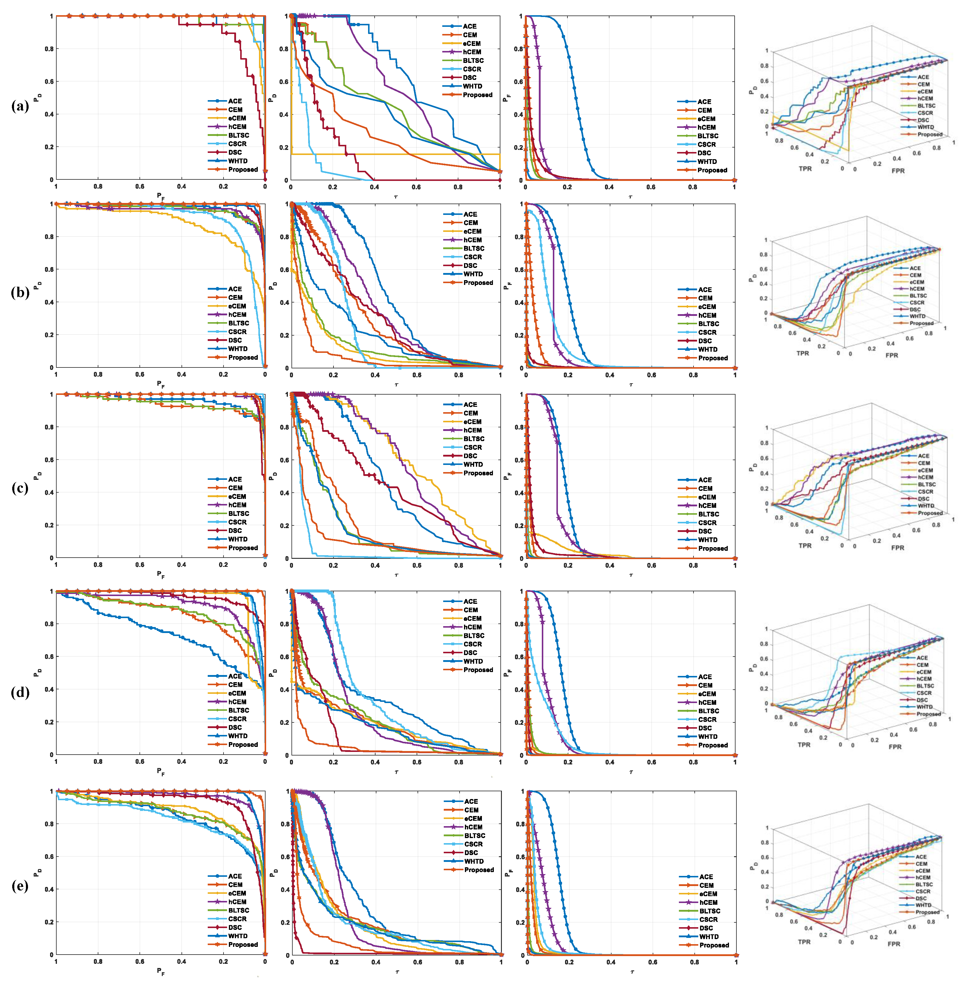
Figure 5 and Figure 6 present the 3D ROC of different methods on five data sets. When the ROC curves reach the upper range of the figure, the detector’s performance improves. The ROC curves of the proposed method surpass others for the San Diego Data Set. For HYDICE, the proposed method is above others in the low region. It is superior to others for the ABU-1, ABU-2, and ABU-3 Data Sets. The hCEM is preferable to others in the high- area, which is usually significant in practical applications. As ROC curves reach the upper limits, detector performance improves significantly. For the San Diego Data Set, the ROC curves of the proposed method outperform others. Higher values in these metrics indicate better detection performance. The AUC of directly correlates with background suppression, with smaller values indicating superior performance. Similarly, assesses detector effectiveness under the joint hypotheses and , while and characterize target detectability and background suppression under single hypotheses, respectively.
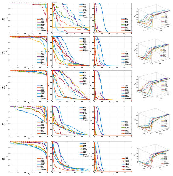
Figure 5.
The 3D ROC curves of different detectors on (a) HYDICE, (b) San Diego, (c) ABU−1, (d) ABU−2, and (e) ABU−3.
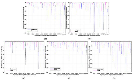
Figure 6.
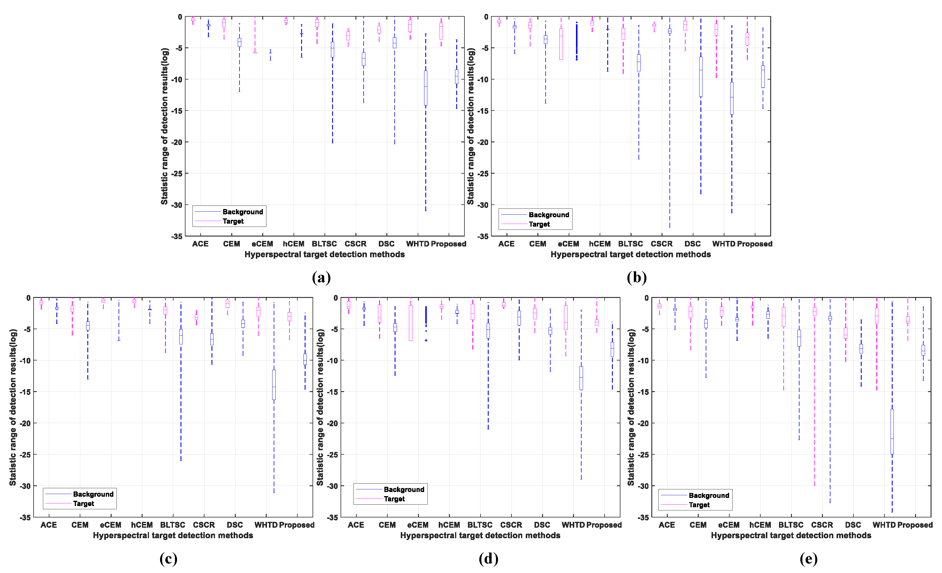
The separability analysis of different detectors on (a) HYDICE, (b) San Diego, (c) ABU−1, (d) ABU−2, and (e) ABU−3.
The AUC of and positively correlates with the detection performance. The higher the value of these two metrics, the better the detection performance. While the AUC of is directly related to background suppression performance, the smaller the value, the better the background suppression performance. So it can also represent good detection performance. The index negatively correlates with the detection performance. characterizes the effectiveness of the detector under the joint hypothesis and . is used to characterize target detectability under the single hypothesis . was used to characterize the background suppression under the single hypothesis .
Taking the ABU-1 data set as an example, in Figure 5 and Figure 6, those different methods have different 3D ROC values. For the 2D ROC curve of , as the abscissa increases, the ordinate decreases accordingly. For the same , the proposed algorithm has a smaller value of than other algorithms. For the 2D ROC curve of , for the same , the proposed algorithm has a higher value of than other algorithms, which reflects the fact that the detection accuracy is higher under the same threshold. For the 2D ROC curve of , the proposed algorithm has a smaller value of than other algorithms for the same , which reflects the fact that the proposed algorithm has fewer misdetections of targets with the same threshold. For the 3D ROC curve, the proposed algorithm achieves a higher curve value in the spatial dimension, meaning better detection performance.
4.5.4. Analysis of Contrast
Figure 6 illustrates the proposed method’s separability abilities with a box plot figure. It can be observed from Figure 6 that the sparse contrast between the tiny target and the intricate background makes it challenging to gather accurate edge and shape information. In the proposed method, the target and background have a more aggregated concentration and a clear differentiation, respectively.
4.5.5. McNemar Test
We performed the McNemar test on the detection results of the HYDICE dataset. The McNemar test is a non-parametric statistical test for paired samples, commonly used to compare categorical variables (such as ’yes/no’ or ’success/failure’) under two different conditions for the same group of subjects.
The McNemar test statistic follows a chi-square distribution with one degree of freedom. To determine whether to reject the null hypothesis, the calculated chi-square statistic is compared to the critical value from the chi-square distribution. If the p-value is less than the significance level (e.g., 0.05), the null hypothesis is rejected, indicating a significant difference in success rates under the two conditions. The test statistic, which is the chi-square value from the McNemar test, indicates the degree of difference between the success rates. A larger statistic suggests a more pronounced difference between the two conditions.
We can observe from Table 8 that the investigated algorithms are statistically significant according to the p-value and statistic.

Table 8.
Statistical analysis on the HYDICE Data Set.
4.6. Ablation Study
Ablation studies evaluate GCN, GAN, fusion strategy, input frequency components, and small batch training patterns to assess their contributions to detection performance.
4.6.1. Analysis of Graph and Generative Learning
Using graph and generative learning modules compared to traditional detection has better performance. Table 9 shows the ablation study results of the two modules quantitatively. If we solely use GAN to locate targets, although possessing attractive detection precision, there is a higher false alarm rate. Moreover, visually, some targets get lost in a cluttered background, which can be seen in Figure 7. Additionally, the incorporation of GCN enhances the precision of detection despite slight misdetection, as seen in Table 9.

Table 9.
Ablation comparison of each module on five data sets.
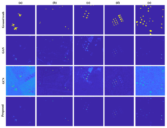
Figure 7.
Component analysis for the (a) HYDICE, (b) San Diego, (c) ABU-1, (d) ABU-2, and (e) ABU-3.
For the ABU-2 dataset, the generative learning module enhances GCN performance significantly, while the fusion module marginally improves accuracy due to noise interference. Similar trends are observed in AUC indicators, reflecting the dataset’s susceptibility to surrounding noise. The generative network can better represent the spatial and spectral information, and the supplementary role of GCN to model the topological information is relatively tiny.
The false alarm rate for detecting discrete targets in the ABU-3 Data Set is relatively high, and GCN’s spectral distortion is severe. Therefore, the fused result improves the detection performance of GCN, but the generative network module performs better. Meanwhile, the separation effect of GAN on the target and the background is also not significant, and the improvement of the fusion effect is limited. However, the generative learning module can also better model the spatial–spectral relationship, and the graph convolution module can detect the target’s spatial position.
For the HYDICE, San Diego, and ABU-1 Data Sets, the fusion improves the results of using only the graph or the generative modules. To summarize, each module impacts detection performance, and most combinations provide beneficial outcomes, indicating how they supplement each other.
4.6.2. Analysis of Number of Training Samples
Across the HYDICE, San Diego, and ABU-1 Data Sets, fusion improves results compared to using individual graph or generative modules. Exploration into sample size impact reveals optimal performance at 30% input, balancing indicator values and computational efficiency. Increasing sample size escalates computation time proportionally, underscoring the efficiency of small batch processing. To explore the impact of the input sample number, we input the training samples of different proportions into the GCN module. Table 10 shows that the input sample ratio has an impact on detection accuracy, false alarm rate, and calculation time. When the input percentage is 30%, the indicator value reaches a reasonable level, while the calculation time is not very high.

Table 10.
Ablation study of the impact of Input samples percentage on the ABU-3 Data Set.
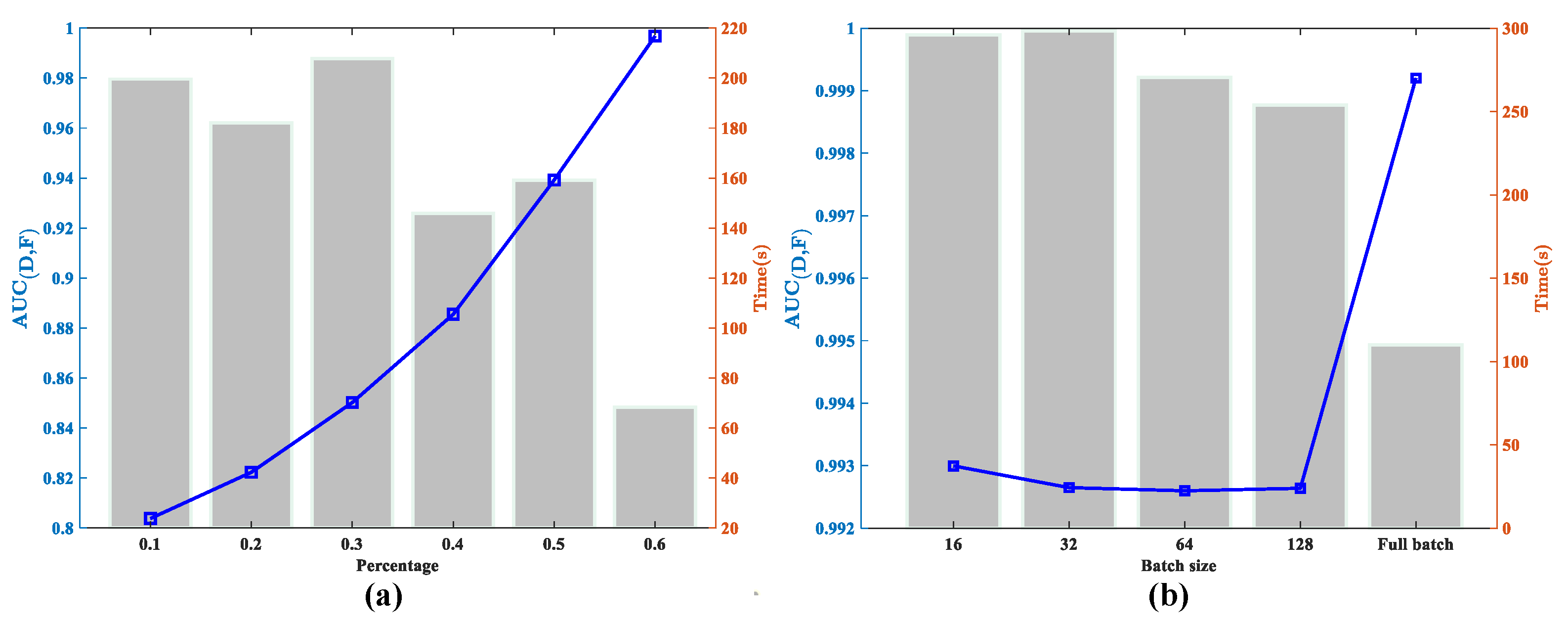
Figure 8a shows the relationship between the percentage of input data with and the relative running time. It can be observed that when the input sample ratio is changed, the accuracy varies between 0.8 and 1, and the accuracy reaches its best when it is 30%. The running time is proportional to the sample size, and as the number of samples increases, the running time shows a more noticeable increase trend. Therefore, we choose an appropriate proportion of input samples to balance the accuracy and the computational cost.
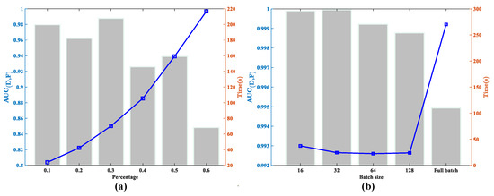
Figure 8.
Effects of (a) percentage of input samples and (b) batch size with and computational cost. The and time are indicated with line and bar charts, respectively.
Simple traditional algorithms, such as the RX detector and CEM, are relatively straightforward with lower computational demands, allowing for faster data processing. They can often achieve near real-time performance. In contrast, complex machine learning or deep learning algorithms, such as neural-network-based target detection methods like models based on GANs, have higher computational complexity and longer processing times, especially in the absence of hardware acceleration. For aerial monitoring systems, such as drones or satellites, the processing time is typically required to be at the second level to quickly identify targets. In ground-based remote sensing applications, the processing time may be relaxed to the minute level, as these scenarios generally have lower real-time requirements compared to aerial platforms.
4.6.3. Effectiveness of Various Aggregations
In Table 11, different fusion strategies are compared to evaluate the effectiveness of the proposed fusion strategy.

Table 11.
Ablation study of the impact of the fusion strategy on the ABU-3 Data Set.
As can be seen from Table 11, although the index of the proposed algorithm on and is slightly worse than the other two methods, it is better than additive fusion and dot production on and . The dot product is used for element-wise multiplication operations, which can preserve the dimensional characteristics of matrices or vectors while introducing fine-grained, element-level control. The addition operation directly adds corresponding elements and is suitable for processing linear combination problems, superimposing information, or performing simple data fusion. The proposed method employs a fusion technique similar to the activation function (exponential function) to merge features extracted through the graph neural network and the generative network. This can be regarded as a combination of a dot product and a nonlinear activation function. After feature extraction, a nonlinear suppression function processes the data, which enhances the model’s nonlinear capabilities and provides a certain aggregation ability for difficult-to-detect targets. In the output results, target information will be improved, the background will be suppressed, and more attention will be given to target pixels, thereby yielding better detection results. Therefore, the proposed fusion method proves to be more effective than additive and dot production fusion.
4.6.4. Analysis of Small Batch Training Strategy
Figure 8b shows the visualization of the relationship between and batch size.
It can be seen from Figure 8b that when the number of batches increases, the does not vary a lot, but the consumption of computing resources is very different. When putting the whole batch into the network, the calculation time is several times that of the small batch. When the batch is set to 32, a balance is achieved between the accuracy and the running time. Table 12 shows that using a small batch pattern of GCN significantly improves computational time compared to the full batch.

Table 12.
Ablation study of the impact of batch size on the HYDICE Data Set.
5. Conclusions
In this article, we focus on the problem of low contrast and imbalance between the target and background, as well as the high computation cost caused by spatial redundancy with high spectral dimensions in target detection on HSIs. To solve the problems, we propose and investigate a deep representative learning model, a two-stream learning pattern consisting of the GCN and the GAN with feature compensation. In particular, the GCN and GAN modules capture and combine the irregular topological and spatial–spectral data to detect small targets in HSIs. Moreover, the designed filter aggregates targets, suppresses the background, and generates pseudo labels for better results, as it enhances the targets. The experimental results on five different HSI data sets show that the proposed method performs better than other state-of-the-art methods, especially in background suppression ability. In the future, we will explore the joint optimization of generative models, and discuss the generalization ability on different data sets.
Author Contributions
Methodology, Y.L., J.Z. and W.X.; software, J.Z., W.X. and P.G.; formal analysis, Y.L., W.X. and P.G.; writing—original draft preparation, J.Z.; supervision, Y.L., W.X. and P.G. All authors have read and agreed to the published version of the manuscript.
Funding
This work was supported in part by the National Natural Science Foundation of China under Grant No. 62121001 and Grant No. U22B2014, in part by Young Elite Scientist Sponsorship Program by the China Association for Science and Technology under Grant 2020QNRC001, and in part by China Scholarship Council No. 202206960021.
Data Availability Statement
The original data presented in the study are included in the article and are also available from the corresponding author.
Acknowledgments
We thank the researchers who provided the experimental data and comparison methods.
Conflicts of Interest
The authors declare no conflicts of interest.
References
- Chang, C.; Ren, H.; Chiang, S. Real-Time Processing Algorithms for Target Detection and Classification in Hyperspectral Imagery. IEEE Trans. Geosci. Remote Sens. 2001, 39, 760–768. [Google Scholar] [CrossRef]
- Chang, C. Hyperspectral Target Detection: Hypothesis Testing, Signal-to-Noise Ratio, and Spectral Angle Theories. IEEE Trans. Geosci. Remote Sens. 2021, 60, 1–23. [Google Scholar] [CrossRef]
- Manolakis, D. Taxonomy of Detection Algorithms for Hyperspectral Imaging Applications. Opt. Eng. 2005, 44, 066403. [Google Scholar] [CrossRef]
- Li, Y.; Shi, Y.; Wang, K.; Xi, B.; Li, J.; Gamba, P. Target Detection with Unconstrained Linear Mixture Model and Hierarchical Denoising Autoencoder in Hyperspectral Imagery. IEEE Trans. Image Process. 2022, 31, 1418–1432. [Google Scholar] [CrossRef]
- Yao, C.; Yuan, Y.; Jiang, Z. Self-Supervised Spectral Matching Network for Hyperspectral Target Detection. In Proceedings of the IEEE International Geoscience and Remote Sensing Symposium (IGARSS2021), Brussels, Belgium, 11–16 July 2021; pp. 2524–2527. [Google Scholar] [CrossRef]
- Chang, C. Hyperspectral Data Processing: Algorithm Design and Analysis; John Wiley & Sons: Hoboken, NJ, USA, 2013. [Google Scholar]
- Rao, W.; Gao, L.; Qu, Y.; Sun, X.; Zhang, B.; Chanussot, J. Siamese Transformer Network for Hyperspectral Image Target Detection. IEEE Trans. Geosci. Remote Sens. 2022, 60, 1–19. [Google Scholar] [CrossRef]
- Harsanyi, J.; Chang, C. Hyperspectral Image Classification and Dimensionality Reduction: An Orthogonal Subspace Projection Approach. IEEE Trans. Geosci. Remote Sens. 1994, 32, 779–785. [Google Scholar] [CrossRef]
- Kraut, S.; Louis, L.; Ronald, W. Adaptive subspace detectors. IEEE Trans. Signal Process. 2001, 49, 3005–3014. [Google Scholar] [CrossRef]
- Yang, S.; Shi, Z. SparseCEM and SparseACE for Hyperspectral Image Target Detection. IEEE Geosci. Remote Sens. Lett. 2014, 11, 2135–2139. [Google Scholar] [CrossRef]
- Chen, L.; Liu, J.; Sun, S.; Chen, W.; Du, B.; Liu, R. An Iterative GLRT for Hyperspectral Target Detection Based on Spectral Similarity and Spatial Connectivity Characteristics. IEEE Trans. Geosci. Remote Sens. 2023, 61, 1–11. [Google Scholar] [CrossRef]
- Kraut, S.; Louis, L.; Ronald, W. The Adaptive Coherence Estimator: A Uniformly Most-Powerful-Invariant Adaptive Detection Statistic. IEEE Trans. Signal Process. 2005, 53, 427–438. [Google Scholar] [CrossRef]
- Robey, F.; Fuhrmann, D.; Kelly, E.; Nitzberg, R. A CFAR Adaptive Matched Filter Detector. IEEE Trans. Aerosp. Electron. Syst. 1992, 28, 208–216. [Google Scholar] [CrossRef]
- Kraut, S.; Scharf, L. The CFAR Adaptive Subspace Detector is a Scale-Invariant GLRT. IEEE Trans. Signal Process. 1999, 47, 2538–2541. [Google Scholar] [CrossRef]
- Harsanyi, J.C. Detection and Classification of Subpixel Spectral Signatures in Hyperspectral Image Sequences. Ph.D. Dissertation, University of Maryland, College Park, MD, USA, 1993. [Google Scholar]
- Farrand, W. Mapping the distribution of mine tailings in the Coeurd’Alene River Valley, Idaho, through the use of a constrained energy minimization technique. Remote Sens. Environ. 1997, 59, 64–76. [Google Scholar] [CrossRef]
- Zou, Z.; Shi, Z. Hierarchical Suppression Method for Hyperspectral Target Detection. IEEE Trans. Geosci. Remote Sens. 2015, 54, 330–342. [Google Scholar] [CrossRef]
- Zhao, R.; Shi, Z.; Zou, Z.; Zhang, Z. Ensemble-based Cascaded Constrained Energy Minimization for Hyperspectral Target Detection. Remote Sens. 2019, 11, 1310. [Google Scholar] [CrossRef]
- Yang, X.; Jie, C.; Zhe, H. Sparse-Spatial CEM for Hyperspectral Target Detection. IEEE J. Sel. Top Appl. Earth. Obs. Remote Sens. 2019, 12, 2184–2195. [Google Scholar] [CrossRef]
- Zhu, D.; Du, B.; Zhang, L. Single-Spectrum-Driven Binary-Class Sparse Representation Target Detector for Hyperspectral Imagery. IEEE Trans. Geosci. Remote Sens. 2020, 59, 1487–1500. [Google Scholar] [CrossRef]
- Li, W.; Du, Q.; Zhang, B. Combined Sparse and Collaborative Representation for Hyperspectral Target Detection. Pattern Recognit. 2015, 48, 3904–3916. [Google Scholar] [CrossRef]
- Shen, D.; Ma, X.; Wang, H.; Liu, J. A Dual Sparsity Constrained Approach for Hyperspectral Target Detection. In Proceedings of the The International Geoscience and Remote Sensing Symposium 2022 (IGARSS2022), Kuala Lumpur, Malaysia, 17–22 July 2022; pp. 1963–1966. [Google Scholar]
- Jiao, C.; Yang, B.; Liu, L.; Chen, C.; Chen, X.; Yang, W.; Jiao, L. Semantic Modeling of Hyperspectral Target Detection with Weak Labels. Signal Process. 2023, 209, 109016. [Google Scholar] [CrossRef]
- Kwon, H.; Nasrabadi, N. Kernel Spectral Matched Filter for Hyperspectral Imagery. Int. J. Comput. Vis. 2007, 71, 127–141. [Google Scholar] [CrossRef]
- Wang, Y.; Chen, X.; Wang, F.; Song, M.; Yu, C. Meta-Learning Based Hyperspectral Target Detection Using Siamese Network. IEEE Trans. Geosci. Remote Sens. 2022, 60, 1–13. [Google Scholar] [CrossRef]
- Xie, W.; Yang, J.; Lei, J.; Li, Y.; Du, Q.; He, G. SRUN: Spectral Regularized Unsupervised Networks for Hyperspectral Target Detection. IEEE Trans. Geosci. Remote Sens. 2020, 58, 1463–1474. [Google Scholar] [CrossRef]
- Shi, Y.; Li, J.; Zheng, Y.; Xi, B.; Li, Y. Hyperspectral Target Detection with RoI Feature Transformation and Multiscale Spectral Attention. IEEE Trans. Geosci. Remote Sens. 2021, 59, 5071–5084. [Google Scholar] [CrossRef]
- Xie, W.; Zhang, X.; Li, Y.; Wang, K.; Du, Q. Background Learning Based on Target Suppression Constraint for Hyperspectral Target Detection. IEEE J. Sel. Top Appl. Earth. Obs. Remote Sens. 2020, 13, 5887–5897. [Google Scholar] [CrossRef]
- Qin, H.; Xie, W.; Li, Y.; Jiang, K.; Lei, J.; Du, Q. Weakly Supervised Adversarial Learning via Latent Space for Hyperspectral Target Detection. Pattern Recognit. 2023, 135, 109125. [Google Scholar] [CrossRef]
- Kipf, T.; Welling, M. Semi-Supervised Classification with Graph Convolutional Networks. arXiv 2016, arXiv:1609.02907. [Google Scholar]
- Wu, Z.; Pan, S.; Chen, F.; Long, G.; Zhang, C.; Philip, S. A Comprehensive Survey on Graph Neural Networks. IEEE Trans. Neural Netw. Learn. Syst. 2020, 32, 4–24. [Google Scholar] [CrossRef]
- Hong, D.; Gao, L.; Yao, J.; Zhang, B.; Plaza, A.; Chanussot, J. Graph Convolutional Networks for Hyperspectral Image Classification. IEEE Trans. Geosci. Remote Sens. 2020, 59, 5966–5978. [Google Scholar] [CrossRef]
- Dong, Y.; Liu, Q.; Du, B.; Zhang, L. Weighted Feature Fusion of Convolutional Neural Network and Graph Attention Network for Hyperspectral Image Classification. IEEE Trans. Image Process. 2022, 31, 1559–1572. [Google Scholar] [CrossRef] [PubMed]
- Dong, Y.; Shi, W.; Du, B.; Hu, X.; Zhang, L. Asymmetric Weighted Logistic Metric Learning for Hyperspectral Target Detection. IEEE Trans. Cybern. 2021, 52, 11093–11106. [Google Scholar] [CrossRef]
- Xu, Y.; Du, B.; Zhang, L. Robust Self-Ensembling Network for Hyperspectral Image Classification. IEEE Trans. Neural Netw. Learn. Syst. 2022, 35, 3780–3793. [Google Scholar] [CrossRef]
- Xu, K.; Qin, M.; Sun, F.; Wang, Y.; Chen, Y.; Ren, F. Learning in the Frequency Domain. In Proceedings of the IEEE/CVF Conference on Computer Vision and Pattern Recognition (CVPR2022), Seattle, WA, USA, 13–19 June 2020. [Google Scholar]
- Takikawa, T.; Acuna, D.; Jampani, V.; Fidler, S. Gated-scnn: Gated Shape CNNs for Semantic Segmentation. In Proceedings of the IEEE/CVF International Conference on Computer Vision (ICCV), Seoul, Republic of Korea, 27 October–2 November 2019; pp. 5229–5238. [Google Scholar]
- Bo, D.; Wang, X.; Shi, C.; Shen, H. Beyond Low-Frequency Information in Graph Convolutional Networks. In Proceedings of the AAAI Conference on Artificial Intelligence (AAAI-21), virtually, 2–9 February 2021; pp. 3950–3957. [Google Scholar]
- Niepert, M.; Ahmed, M.; Kutzkov, K. Learning Convolutional Neural Networks for Graphs. In Proceedings of the 33nd International Conference on Machine Learning (ICML), New York City, NY, USA, 19–24 June 2016; pp. 2014–2023. [Google Scholar]
- Zeng, H.; Zhou, H.; Srivastava, A.; Kannan, R.; Prasanna, V. Graphsaint: Graph Sampling Based Inductive Learning Method. arXiv 2019, arXiv:1907.04931. [Google Scholar]
- Chang, C. An Effective Evaluation Tool for Hyperspectral Target Detection: 3D Receiver Operating Characteristic Curve Analysis. IEEE Trans. Geosci. Remote Sens. 2020, 59, 5131–5153. [Google Scholar] [CrossRef]
Disclaimer/Publisher’s Note: The statements, opinions and data contained in all publications are solely those of the individual author(s) and contributor(s) and not of MDPI and/or the editor(s). MDPI and/or the editor(s) disclaim responsibility for any injury to people or property resulting from any ideas, methods, instructions or products referred to in the content. |
© 2024 by the authors. Licensee MDPI, Basel, Switzerland. This article is an open access article distributed under the terms and conditions of the Creative Commons Attribution (CC BY) license (https://creativecommons.org/licenses/by/4.0/).

