Article

Examining the Impact of Topography and Vegetation on Existing Forest Canopy Height Products from ICESat-2 ATLAS/GEDI Data

1
Key Laboratory for Humid Subtropical Eco-Geographical Processes of the Ministry of Education, Fujian Normal University, Fuzhou 350117, China
2
Institute of Geography, Fujian Normal University, Fuzhou 350117, China
3
Institute of East China Inventory and Planning, National Forestry and Grassland Administration, Hangzhou 310019, China
*
Author to whom correspondence should be addressed.
Remote Sens. 2024, 16(19), 3650; https://doi.org/10.3390/rs16193650
Submission received: 21 August 2024 / Revised: 27 September 2024 / Accepted: 27 September 2024 / Published: 30 September 2024
(This article belongs to the Special Issue Lidar for Forest Parameters Retrieval)

Abstract

:
Forest canopy height (FCH) is an important variable for estimating forest biomass and ecosystem carbon sequestration. Spaceborne LiDAR data have been used to create wall-to-wall FCH maps, such as the forest tree height map of China (FCHChina), Global Forest Canopy Height 2020 (GFCH2020), and Global Forest Canopy Height 2019 (GFCH2019). However, these products lack comprehensive assessment. This study used airborne LiDAR data from various topographies (e.g., plain, hill, and mountain) to assess the impacts of different topographical and vegetation characteristics on spaceborne LiDAR-derived FCH products. The results show that GEDI–FCH demonstrates better accuracy in plain and hill regions, while ICESat-2 ATLAS–FCH shows superior accuracy in the mountainous region. The difficulty in accurately capturing photons from sparse tree canopies by ATLAS and the geolocation errors of GEDI has led to partial underestimations of FCH products in plain areas. Spaceborne LiDAR FCH retrievals are more accurate in hilly regions, with a root mean square error (RMSE) of 4.99 m for ATLAS and 3.85 m for GEDI. GEDI–FCH is significantly affected by slope in mountainous regions, with an RMSE of 13.26 m. For wall-to-wall FCH products, the availability of FCH data is limited in plain areas. Optimal accuracy is achieved in hilly regions by FCHChina, GFCH2020, and GFCH2019, with RMSEs of 5.52 m, 5.07 m, and 4.85 m, respectively. In mountainous regions, the accuracy of wall-to-wall FCH products is influenced by factors such as tree canopy coverage, forest cover types, and slope. However, some of these errors may stem from directly using current ATL08 and GEDI L2A FCH products for mountainous FCH estimation. Introducing accurate digital elevation model (DEM) data can improve FCH retrieval from spaceborne LiDAR to some extent. This research improves our understanding of the existing FCH products and provides valuable insights into methods for more effectively extracting accurate FCH from spaceborne LiDAR data. Further research should focus on developing suitable approaches to enhance the FCH retrieval accuracy from spaceborne LiDAR data and integrating multi-source data and modeling algorithms to produce accurate wall-to-wall FCH distribution in a large area.

1. Introduction

Forest canopy height (FCH) is an important variable for use in modeling forest carbon stocks or growing stock volume, which are crucial indicators for evaluating the productivity of forest ecosystems [1,2,3]. Traditionally, tree height is measured using telescopic poles or laser rangefinders, but it is often difficult to accurately measure tree heights in densely forested areas [4]. Light detection and ranging (LiDAR) technology makes it possible to estimate tree height [5]. In particular, spaceborne LiDAR has become an important data source to map FCH at national and global scales [6,7,8].
The ice, cloud, and land elevation satellite-2 (ICESat-2) is equipped with a photon-counting LiDAR (PCL) instrument called the advanced terrain laser altimeter system (ATLAS) [9]. ATLAS uses a high pulse repetition rate and multi-beam detection (including three strong beams and three weak beams), able to obtain a footprint with a diameter about 11–12 m on the ground and high-density photon point cloud data with 0.7 m sampling interval between footprints along ground tracks [9]. The Global Ecosystem Dynamics Investigation (GEDI) is a full-waveform LiDAR instrument that collects observations of vertical structures over earth’s surface between 51.6° north and south latitude [10]. The GEDI LiDAR system instrument consists of three lasers: two full power beams and one split into two coverage beams. Each laser emits 242 times per second, resulting in 25 m average diameter footprints that are separated by 60 m along the track [10]. Both ATLAS and GEDI play an important role in mapping vegetation and forest height globally, as well as estimating forest carbon stocks [11,12]. One shortcoming of spaceborne LiDAR data is that they cannot provide a spatially continuous FCH product without incorporating other remotely sensed data [13,14]. The previous research has explored the combined use of spaceborne LiDAR and optical or synthetic aperture radar (SAR) data for modeling FCH or aboveground biomass distribution [6,15,16,17]. However, the accuracies of these products varied considerably, depending on forest coverage and terrain conditions.
The airborne LiDAR (ALS) canopy height model (CHM), digital surface model (DSM), and digital elevation model (DEM) are often considered to provide accurate measurements and have become the primary validation data for evaluating the spaceborne LiDAR products. Some studies have also used the GEDI simulator [18] and ICESat-2 simulator [19] to simulate the waveform from ALS/TLS (terrestrial laser scanner) as validation data. Terrain height is another important parameter for spaceborne LiDAR products. Terrain height data are available in both ATLAS and GEDI [20,21], and the root-mean square error (RMSE) of terrain heights from ATLAS can be less than 1 m in the best-case scenario [20,22]. However, the evaluation of ATLAS and GEDI results shows that the accuracy of terrain height varies depending on region, time, and beam of data acquisition [23,24,25]. For ATLAS, strong beam nighttime data are more accurate than daytime data because night acquisition does not suffer from the impact of solar background noise [26]. Excessive cloud cover, snow cover, and canopy cover can also decrease terrain height accuracy [22,26,27], and terrain slope considerably affects terrain height retrieval accuracy, especially for GEDI [28].
Factors such as terrain slope, canopy coverage, forest type, and the way of data collection (e.g., strong and weak beams, nighttime and daytime data) may affect spaceborne LiDAR FCH products [20,25]. The previous research has shown that the FCH retrieval accuracy from ATLAS is lower than that of terrain height [26], and GEDI performs better than ATLAS [25]. They are considered capable of providing consistent forest height data to support global forest height mapping [29]. The FCH product from nighttime data exhibits better accuracy than that from daytime data, with RMSE for ATLAS decreasing from 7.21 m to 5.02 m and for GEDI reducing from 3.93 m to 3.56 m [25]. For ATLAS, strong beams receive significantly more photon signals than weak beams; thus, strong beams can better characterize the forest structure [30]. For GEDI, the full-power beams have slightly better data accuracy than the coverage beams [31,32]. Vegetation characteristics (e.g., canopy cover, forest type, and canopy height) also affect FCH products from spaceborne LiDAR [30,33]. Data accuracy tends to diminish under dense canopy cover due to inaccurate terrain height [25]. Terrain slope and snow cover can significantly affect canopy height retrieval accuracy [23,27,34].
Spaceborne LiDAR data alone cannot provide a wall-to-wall FCH product without the incorporation of optical or radar data [6,11,17,35]. Since terrain and vegetation cover vary greatly among plain, hill, and mountain regions, these differences can affect the accuracy of vegetation structure retrieval by the LiDAR system to varying degrees, and they may considerably influence the quality of FCH products from spaceborne LiDAR data. However, it is unclear how different topographic and vegetation conditions affect these data products. Plain regions have flat terrain but often have sparse and discrete vegetation spatial patterns. Mountainous regions show wide variation in topographic and vegetation conditions, while hilly regions have relatively undulating terrain with various patch sizes of vegetation cover. Several global or national wall-to-wall FCH products were generated using different methods based on the integration of ATLAS and/or GEDI with other datasets [6,8,11,17].
This research aims to improve our understanding of the existing FCH product accuracy in different landforms. Thus, three different topographic regions (i.e., plain, hill, and mountain) with various slopes, forest types, and coverages were selected to examine the FCH products from ATLAS and GEDI data alone, as well as the wall-to-wall FCH products.

2. Study Areas and Materials
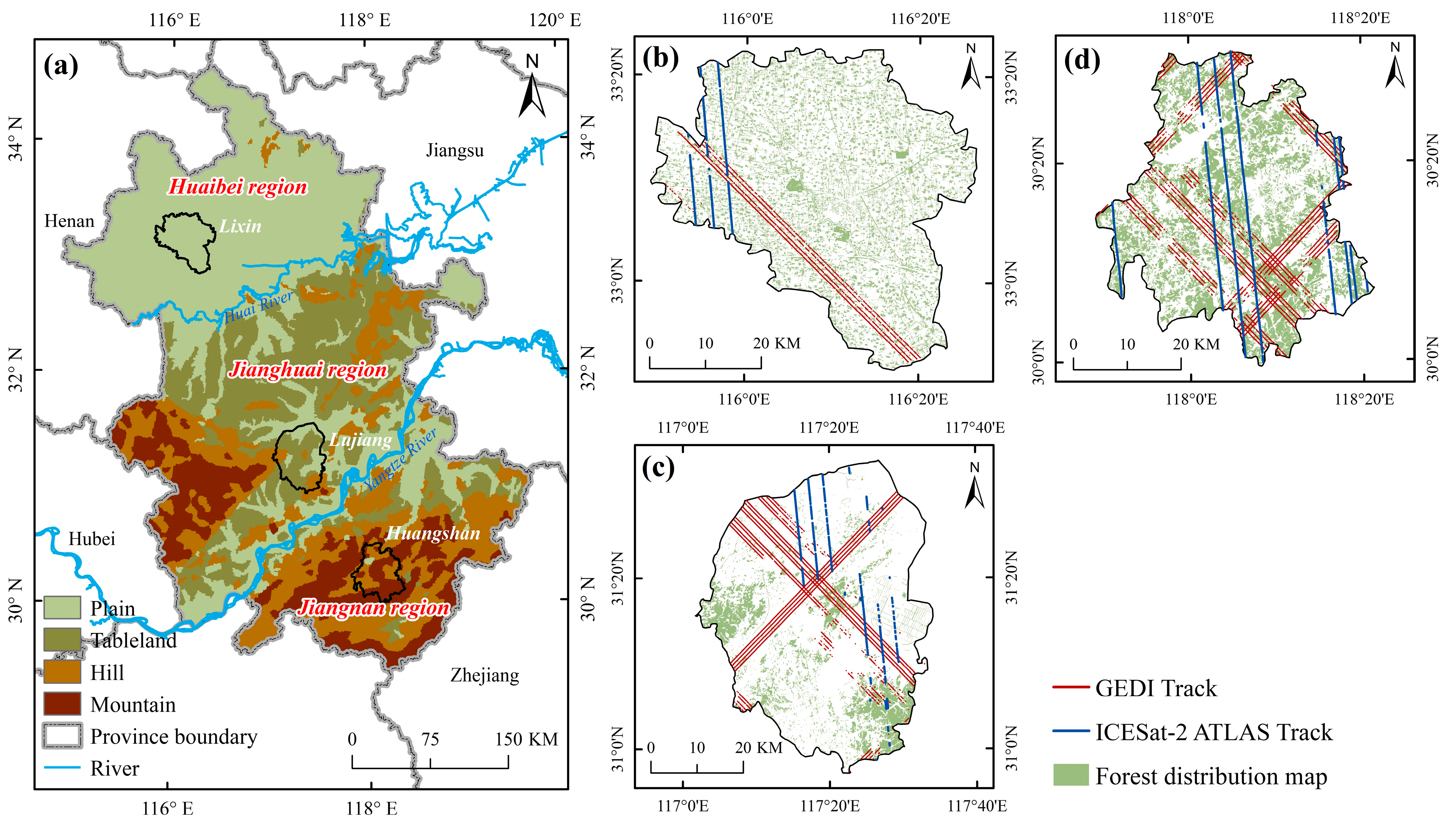
2.1. Study Areas

Three typical regions—Lixin County, Lujiang County, and Huangshan District in Anhui Province—were selected, representing plain, hill, and mountain topographies (See Figure 1). Anhui Province is located at the transition zone between the warm temperate and subtropical regions. The Yangtze and Hui Rivers traverse the province from west to east, dividing it into three distinct topographic regions: Huaibei (north of the Huai River), Jianghuai (between the Yangtze River and the Huai River), and Jiangnan (south of the Yangtze River) (Figure 1a). Huaibei consists of a vast plain with loamy soil, while the Jianghuai and Jiangnan regions are primarily characterized by undulating hills (including tablelands and hills) and mountains. Several mountain ranges run west to east, with Dabie, Huangshan, and Jiuhua being the most geographically renowned mountains for their natural beauty.
Lixin County is situated in the south of Huaibei Region and characterized by a flat topography, the elevation range is 9~57 m. In 2019, Forestlands occupied 4521 ha with poplar being the dominant tree species, and their canopy heights were less than 30 m. Lujiang County in Jianghuai Region has high terrain in the southwest and low in the northeast with an elevation range of −35 to 568 m. Hills account for 72.3% of the county’s area and are mainly distributed in the southeastern, western, and central areas. The forest coverage is 16.68% with dominant tree species including Moso bamboo, Chinese fir, Masson pine, and poplar. Their canopy heights were mainly less than 30 m. Huangshan District in Jiangnan Region is in the middle of the southern Anhui mountainous area with high terrain in the south and low in the north. The general elevation range is between 71 and 1819 m. Due to its unique topography, the vegetation in this region shows obvious vertical distribution characteristics with forest coverage of 80.0%. The dominant forest types include Masson pine, Moso bamboo, Chinese fir, and broadleaf forests, and their canopy heights were mainly less than 35 m.

2.2. Data Collection

The datasets used in this research included FCH products from ATLAS and GEDI, wall-to-wall FCH products, ALS, and other ancillary data. They are summarized in Table 1.

2.2.1. The FCH Products from ICESat-2 ATLAS and GEDI

Among the various types and levels of ATLAS products, ATL03 and ATL08 are most often used in forestry applications. ATL03, known as the global geolocated photon data product, serves as a bridge between lower and higher-level of ATLAS products. It contains the precise time, latitude, longitude, and elevation of every received photon. These photons are classified as either likely signal or background with a confidence assessment, as well as by surface types such as land ice, sea ice, land, ocean, and inland water. ATL08 is a level 3 land/vegetation height product, which includes heights for both terrain and canopy, as well as other descriptive parameters at a fixed step-size of 100 m (a segment) along the track direction. Starting from version 5, 20 m sub-segments with the metric of the 98th percentile height were added to the ATL08 product [30,36]. The 98th percentile height was used to represent the top of the canopy, as it ignored noise data that could cause errors in tree height, and was considered more reliable than the 100th percentile height. ATL08 is derived from ATL03 after a series of complex processing steps, including noising filtering by the differential, regressive, and Gaussian adaptive nearest neighbor (DRAGANN) algorithm, ground and canopy surface finding, top of canopy finding filter, photon classification (four types of photons: noise, ground photons, canopy photons, and top-of-canopy photons), and canopy height determination [19]. In addition, the labeled photons used to determine the data parameters in ATL08 can be indexed back to the ATL03 products. In this study, we obtained ICESat-2 ATL03 and ATL08 products (version 6) that transected Anhui Province during April–October 2019 from the NSIDC ICESat-2 Data Sets website. The previous research has demonstrated that ATLAS nighttime strong beams provided superior data accuracy [20,30]; therefore, only ATLAS nighttime strong beam data were retained for FCH evaluation.
The GEDI L1B product provided raw waveform data from the LiDAR system, capturing the signals returned from the earth’s surface and vegetation, while the GEDI L2A product was a geolocated elevation and height metrics product derived from GEDI L1B received waveform. This product contained 156 attributes for each of the eight beams, including ground elevation, canopy top height, relative height (RH) metrics, and other interpreted products from the return waveforms at a spatial resolution (average footprint) of 25 m. The beam sensitivity parameter reflected the maximum canopy cover that can be penetrated considering the signal-to-noise ratio of the waveform. In this study, only high-quality footprints (i.e., “quality_flag = 1”, “degrade_flag = 0”, and “sensitivity > 0.9”) of the full-power beams were chosen for further analysis, considering their expected accuracy and reliability. Among the various attributes of the L2A product, two variables were selected for GEDI product evaluation: the elev_lowestmode and RH98. The elev_lowestmode contains the elevation of the center of the lowest mode of the footprint waveform relative to the reference ellipsoid (WGS-84). It is generally considered a representation of ground elevation [37]. RH98 represents the height of the 98th percentile of the cumulative waveform energy relative to the ground, used as a proxy for the canopy top height.

2.2.2. Wall-to-Wall FCH Products Generated from Integration of ICESat-2 ATLAS and/or GEDI with Other Datasets

In this study, we assessed three publicly available FCH products (Table 1) in the selected typical regions: (1) Forest Tree Height Map of China (FCHChina) in 2019 [6]; (2) Global Forest Canopy Height Map in 2020 (GFCH2020) [35]; and (3) Global Forest Canopy Height Map in 2019 (GFCH2019) [17]. FCHChina was generated by fusing ATLAS, GEDI, and Sentinel-2 images for the year 2019 using a neural-network-guided interpolation (NNGI) method at a spatial resolution of 30 m. The accuracy was reported as R2 of 0.58 and RMSE of 4.93 m compared to the drone-LiDAR data. GFCH2020 was produced by integrating ATLAS, GEDI, Sentinel-1/2, and other ancillary data using a random forest algorithm. However, accuracy was not reported. GFCH2019 was produced through the integration of GEDI and Landsat analysis-ready data time-series using a regression tree ensemble algorithm, with RMSE of 9.07 m.

2.2.3. Airborne LiDAR (ALS) and Ancillary Data

ALS data for the three study areas were acquired in June 2019 using the RIEGL VQ-1560i-DW LiDAR scanning system mounted on an aircraft. This LiDAR system utilized a near-infrared spectral channel, achieving an average point density of 4 points/m2.
Ancillary datasets used in this study include vegetation- and terrain-related data. They are forest distribution map (2019) and NASADEM. The 2019 forest map is a vector dataset containing attributes such as tree species/forest types and terrain types. The forest map was converted into a raster format with a pixel size of 30 m × 30 m, aligning with the wall-to-wall FCH products. The NASADEM with a spatial resolution of 30 m is considered to have better data quality than others (e.g., ASTER GDEM, SRTM DEM) [38], thus, NASADEM covering Anhui Province was used after alignment with the other raster products. The terrain slope was generated from NASADEM and grouped into six levels (0°–10°, 10°–20°, 20°–30°, 30°–40°, 40°–50°, 50°–60°).

3. Methods

In this research, the spaceborne LiDAR FCH products and wall-to-wall FCH products were assessed under different terrain and vegetation conditions. The terrain conditions encompass various topographies (plain, hill, and mountain) and slope categories, while vegetation conditions include different forest and canopy types. According to the slope range (0–60°) in the study areas, the slopes were divided into six levels with equal intervals. The canopy cover was grouped into three categories: low (0–40%), medium (40–80%), and high (80–100%).

3.1. Data Processing

3.1.1. Airborne LiDAR Processing

Prior to utilizing the ALS data (Section 2.2.3), they should be preprocessed accordingly. After noise removal, the LiDAR point cloud data were classified into ground points and non-ground points using the triangular irregular network (TIN) densification algorithm. The digital elevation model (DEM) and digital surface model (DSM) were generated from the ground points and non-ground points, respectively, using the TIN interpolation method. The DEM and DSM data for Lixin and Lujiang were produced at a pixel size of 1 m × 1 m, while for Huangshan, they were produced at a resolution of 2 m × 2 m. Canopy height models (CHM) were calculated by subtracting the DEM from the DSM. A median filter was applied to the CHM to refine it and remove outliers. The 98th percentile canopy heights derived from ALS CHM data were aggregated to match specified sizes corresponding to ICESat-2 segments, GEDI footprints, or the resolution of wall-to-wall FCH products to serve as reference for FCH evaluation.
ALS CHM and DEM data were used to calculate reference values for evaluating spaceborne LiDAR products and the existing wall-to-wall FCH products. For ATLAS and GEDI, approximate footprint extents (20 m × 14 m polygons and 12.5 m-radius circles) were considered as extraction extents, while for wall-to-wall FCH products, a cell size of 30 m × 30 m was used. The 98th percentile height (refers to as ALS FCH hereafter) and the mean of DEM within the corresponding extraction extents were computed. The sum of the ALS FCH and the mean DEM was then used as a reference value for ALS DSM.
To analyze the impact of vegetation cover conditions on the accuracy of FCH products, canopy cover was calculated, considering that different canopy covers may affect the ability of laser beams to reach the ground or capture forest structures. Canopy cover is typically defined as the ratio of the vegetation-covered area to the total area of a specified size. In this study, we defined canopy cover (Formula (1)) as the ratio of the number of ALS CHM cells with height greater than 2 m to the total number of grids within certain extents (footprints and 30 m × 30 m pixels). Based on these calculations, canopy cover was classified into three levels: low (0–40%), medium (40–80%), and high (80–100%).
C a n o p y   C o v e r = N C H M > 2 m N t o t a l
where N C H M > 2 m represents the number of ALS CHM cells with height greater than 2 m in the certain extents, and N t o t a l represents the total number of ALS CHM cells in the certain extents [25,26].

3.1.2. ICESat-2 ATLAS and GEDI Data Processing

The ICESat-2 ATL08 metrics, derived from the aggregation of photons over the segments, and GEDI L2A data, derived from return waveforms, were assigned to the central locations (longitude and latitude) as attributes. It is necessary to determine the actual geographical extents corresponding to these metrics based on their central locations. This process is known as data spatialization.
For ATLAS data, the spatializing segments of 20 m in length involves the following steps:
  • Linking ATL08 to ATL03: The ATL08 product stores photon classifications used in the calculated height metrics for a 20-m segment but lacks geolocation information, while the ATL03 product contains the absolute height and geolocation information of each photon. Geographical coordinates and absolute height of each photon presented in the ATL08 products can be extracted from ATL03 using the group number (“ph_segment_id = segment_id”). In this process, we extracted the longitude and latitude from ATL03 for each photon within ATL08 segments of the selected nighttime strong beams;
  • Connecting the first and last observation for each 20-m segment to form the centerline of the segment;
  • Creating 20 m × 14 m ATLAS footprints along the centerlines of segments: If the centerline length is 20 m, a 7-m buffer was created on both sides; if a centerline was less than 20 m, it was extended to 20 m (10 m on each side from its midpoint), and then a buffer of 7 m was created on both sides;
  • The FCH of 20 m-segment (i.e., the 98th percentile) in ATL08 was linked to the corresponding 20 m × 14 m footprint as an attribute. Additionally, the sum of the canopy height and ground height (“h_te_best_fit_20m”) was regarded as the elevation at canopy top of the segment, which is equivalent to the DSM. Both the canopy height and DSM were the evaluation subjects of ATLAS products.
For GEDI data, high-quality footprints extracted from GEDI L2A (including coordinates of central points, terrain elevation, and RH98) were spatialized by creating circular buffers with a radius of 12.5 m around the center coordinates (longitude and latitude) of each footprint, with relative height (“RH98”) and ground elevation (“elev_lowestmode”) as attributes. In addition, the sum of RH98 and ground elevation was calculated and used as DSM of the GEDI footprint. RH98 and DSM were the evaluation subjects of the GEDI products. Additionally, this size of ATLAS segment and GEDI footprint are more consistent with the grid size of wall-to-wall FCH maps.
For spaceborne LiDAR products, forest footprints were screened by canopy cover obtained from ALS CHM, and only the forest footprints were retained for analysis. After filtering, the ATLAS dataset contained 610, 1135, and 2848 segments for plain, hill, and mountain regions, respectively, and the GEDI dataset contained 898, 5220, and 9666 footprints, respectively.

3.2. Evaluation Method

3.2.1. Evaluation of Spaceborne LiDAR Data

The impacts of DSM and DEM accuracies on FCH were examined by evaluating profiles of spaceborne LiDAR data. The portions of ATLAS and GEDI tracks with dense vegetation cover were selected, and profile graphs were created to show the elevation of ATL03 photons of different types (canopy photon, top canopy photon, and ground photon), as well as the ground and canopy elevation of GEDI footprints against the ALS DSM and DEM. The agreements between spaceborne LiDAR and ALS data in terms of DSM and DEM were then assessed. The effects of different combinations of canopy cover and terrain conditions (high canopy cover and high slope, high canopy cover and low slope, low canopy cover and high slope, and low canopy cover and low slope) on the accuracy of DSM and DEM of footprints in plain, hill, and mountain regions were explored.
In addition to analyzing the impact of ATLAS photons and GEDI ground or canopy elevation on FCH retrieval, this research also directly evaluates spaceborne LiDAR FCH products in mountainous regions. The accuracy of ATLAS and GEDI FCH products under different canopy covers (low, medium, and high) and terrain slope levels (six slope intervals) were examined using counterparts calculated from ALS data. To eliminate the interference of slope on the analysis of canopy cover, only footprints with a slope below 20° were selected for canopy cover analysis.

3.2.2. Evaluation of Wall-to-Wall FCH Products

For wall-to-wall FCH products, pixels classified as forest were extracted from the forest map, and 8000 points within each study area (Lixin, Lujiang, and Huangshan) were then randomly selected. For each point, the FCH values from different products, as well as the ALS FCH value, slope, canopy cover, and forest type from their respective maps were extracted. The overall accuracies of FCH products in each region were evaluated. For the mountain region (Huangshan District), FCH retrieval accuracies were further examined under different canopy cover levels (high, medium, and low), slope levels (total of 6 levels), and forest types (Masson pine, Chinese fir, Moso bamboo, and broadleaf forests).

3.2.3. Incorporation of Precise DTM and Spaceborne LiDAR DSM for FCH Retrieval

We conducted an experiment in a mountainous region by selecting ATLAS segments and nearby GEDI footprints. The original ATL08 ATBD algorithm still has flaws in filtering noise and classifying non-ground photons [26], leading to some noisy photons being misclassified as canopy photons. Attempting to remove these noisy photons, we used the maximum value of the ALS DSM corresponding to a 20 m segment as a threshold. ATLAS photons with elevation more than 1 m higher than this threshold were eliminated. The percentile statistics, particularly the 98th percentile, were then extracted from the remaining canopy photons based on their elevation differences. Finally, we incorporated the precise DTM and spaceborne LiDAR DSM to extract FCH.

3.2.4. Accuracy Assessments

For each of the evaluation subjects, including DEM, DSM, ATLAS-FCH, GEDI-FCH, and wall-to-wall FCH products, four evaluation measures—root mean square error (RMSE), relative RMSE (rRMSE), mean bias, and R-square (R2)—were calculated using the following equations based on ALS reference data. These metrics were used to estimate accuracy.
R M S E = 1 n i = 1 n ( a i b i ) 2
r R M S E = R M S E b ¯ × 100 %
b i a s = 1 n i = 1 n ( a i b i )
R 2 = 1 i = 1 n a i b i 2 i = 1 n a i b ¯ 2
where a i and b i denote the evaluation subjects and corresponding ALS references, b ¯ is the average of ALS reference values, and n is the number of values involved in calculation.

4. Results

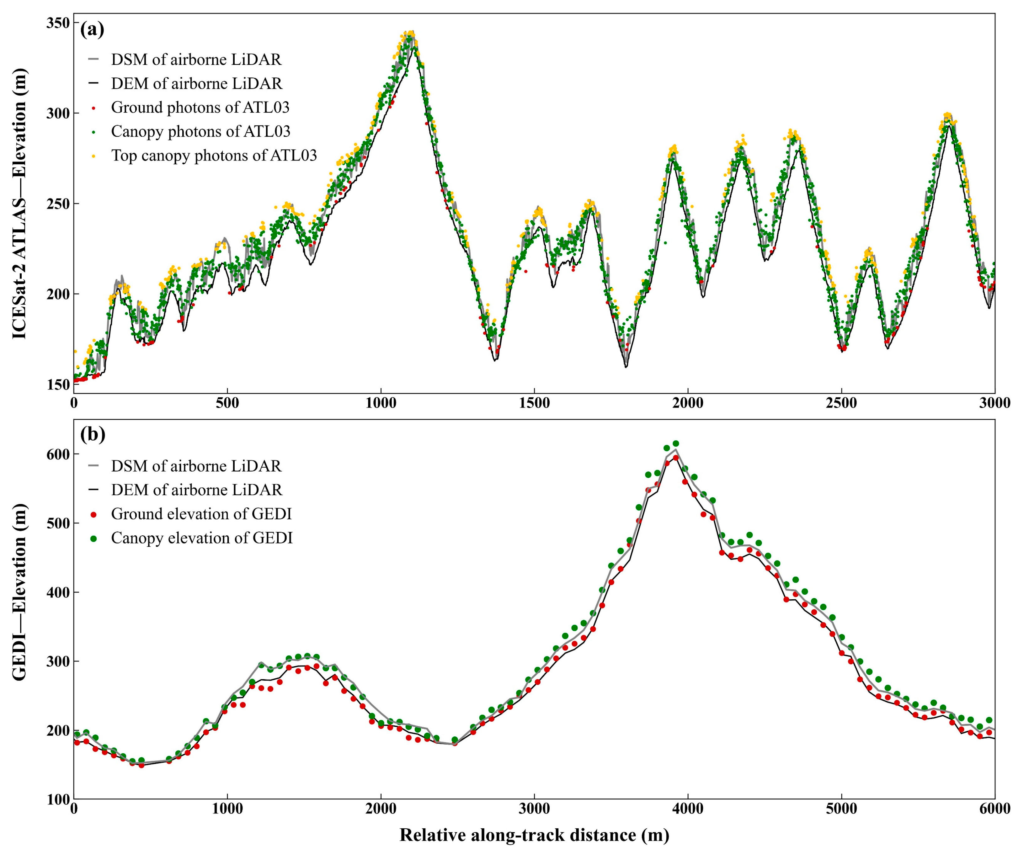
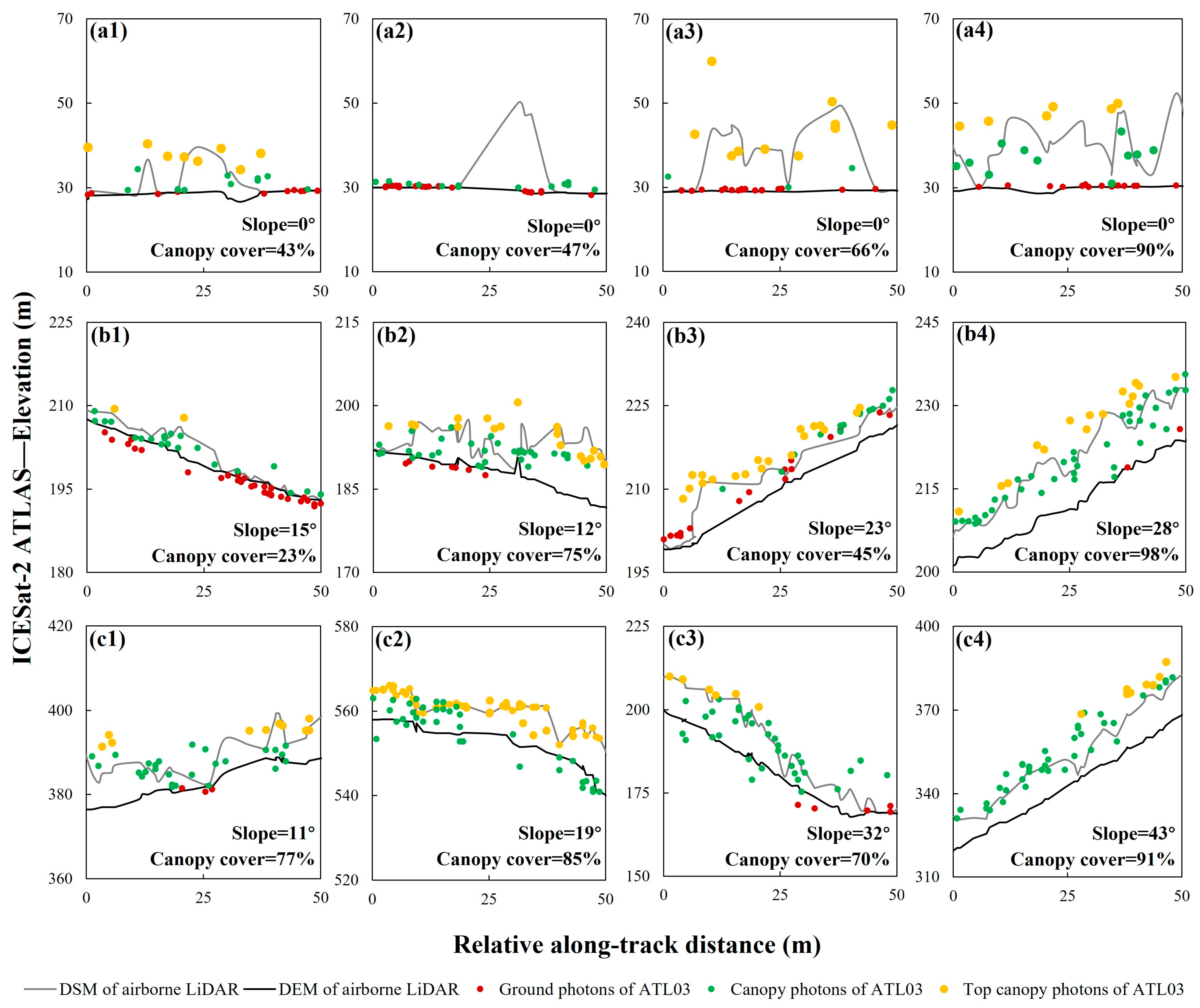
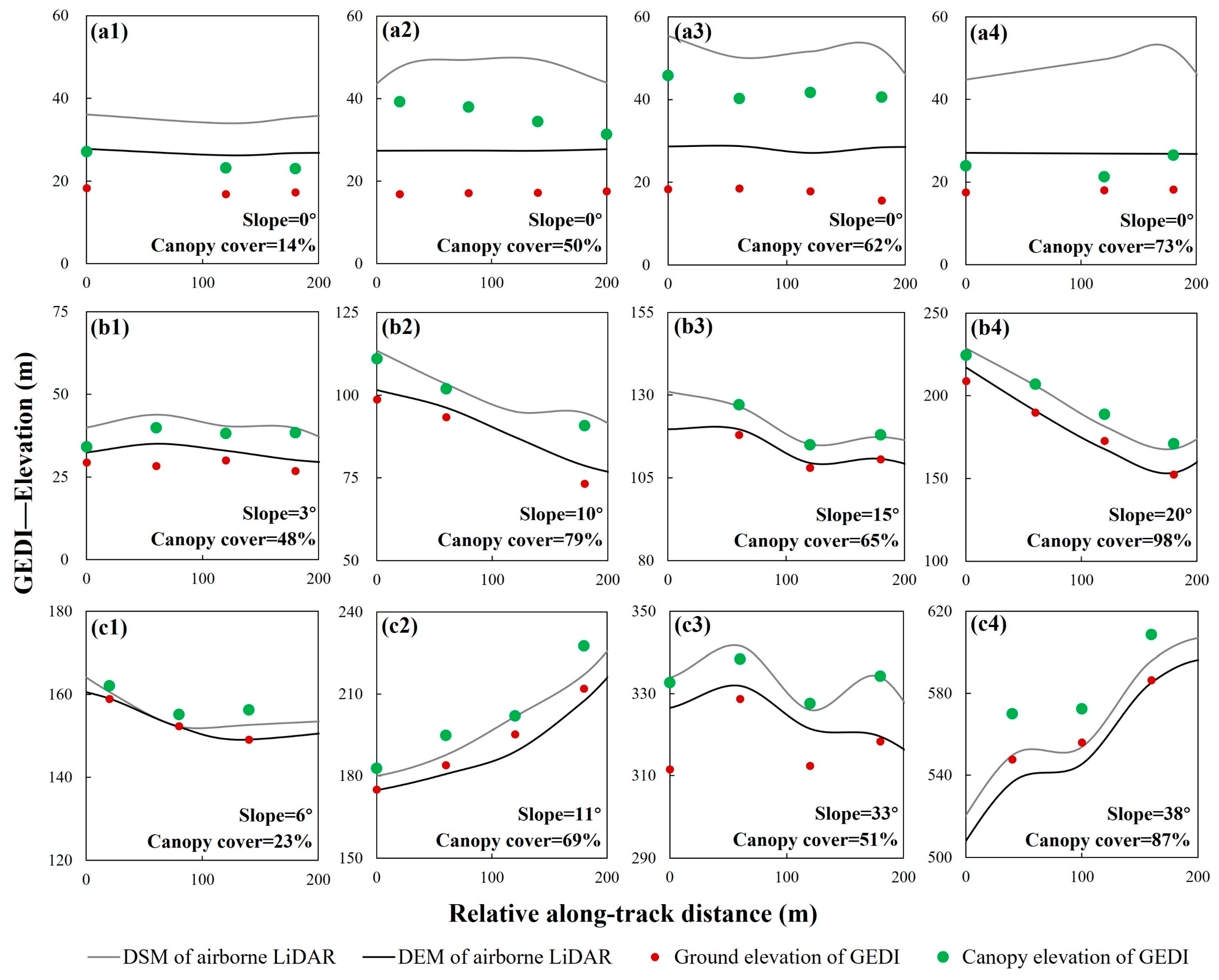
4.1. Evaluation of Canopy Elevation and Ground Elevation of ICESat-2 ATLAS and GEDI Products

The canopy and ground elevation profiles along selected ATLAS and GEDI tracks in a mountainous region (Figure 2) showed that ATLAS ground photons were very sparse under dense canopy cover and steep terrain conditions (only 63 out of the 150 segments in Figure 2a have ground photons), while canopy and top-of-canopy photons were relatively abundant (each segment averages 16.5 canopy photons and 0.9 ground photons). Top-of-canopy photons were mostly concentrated at the top of mountain and very few on slopes. Some canopy photons and top-of-canopy photons were above the ALS DSM (average error: 4.66 m). Discrepancies between GEDI canopy elevation and the ALS DSM were evident within relative distances between 3000 m and 6000 m in Figure 2b, with GEDI DSM being higher than ALS DSM (average error: 8.50 m). Additionally, the ground elevation from GEDI in dense vegetation areas in mountainous region was more comprehensive than that from ATLAS, as it can extract elevation from each footprint’s waveform. Profiles of selected ATLAS and GEDI tracks under different canopy covers and terrain slopes in three study areas demonstrated various patterns in DSM and DEM compared to the ALS counterparts (Figure 3 and Figure 4). These patterns indicated significant impacts of vegetation cover and terrain conditions on the accuracy of spaceborne LiDAR DSM and DEM and, consequently, on the accuracy of FCH retrieval.
Figure 3 shows that ATLAS ground photons were more abundant in the plain and hill regions than in the mountain region. In particular, the ground photons in the plain region (e.g., Lixin County) closely aligned with the ALS DEM, implying the high accuracy of the ATLAS DEM. It was also observed that few or no ground photons were found beneath canopy photons or top-of-canopy photons due to canopy occlusion. Although more high-precision ground photons were present in the plain area, the canopy photons and top-of-canopy photons were prevalent only under high vegetation cover conditions. Additionally, canopy heights for sparse vegetation may not always be obtainable (Figure 3(a1,a2)). This suggests that the FCH is more dependent on canopy cover than on terrain in plain areas, and sparse vegetation negatively impacts the acquisition of canopy photons. In the hill regions (e.g., Lujiang County), there were more high-quality canopy photons than in the plain region, attributed to the relatively dense canopy cover (Figure 3(b1–b4)). The number and quality of photons appeared to be influenced by terrain slope and canopy cover. Higher vegetation cover resulted in fewer ground photons, and steeper slopes caused larger deviations of photons from the actual ALS DSM and DEM, leading to lower FCH retrieval accuracy. The profile of ATLAS photons on the selected track in the mountain region (i.e., Huangshan District) (Figure 3(c1–c4)) showed limited ground photons but abundant canopy photons due to the dense vegetation cover. The number of ground photons was primarily related to the vegetation cover; when it reached a relatively high value such as 85% (Figure 3(c2)), no photons hit the ground. As a result, it is possible to obtain accurate canopy surface height from the abundant canopy photons, but retrieving a high-precision DEM becomes challenging, which affects the computation of accurate FCH. Additionally, the steepness of the terrain slope impacted the classification of photons, as exemplified in Figure 3(c3,c4), where considerable misclassification of canopy photons and top-of-canopy photons occurred on very steep slopes.
The profiles of GEDI footprints (Figure 4) illustrate varying performances in representing elevation. In the plain region, GEDI canopy and ground elevations exhibited noticeably systematic biases compared to ALS data (Figure 4(a1–a4)). However, regardless of vegetation cover, the distance between GEDI canopy elevation and ground elevation consistently aligned with the corresponding ALS DSM and DEM in most cases, demonstrating its capability to provide accurate canopy height. In the hill region (Figure 4(b1–b4)), both GEDI canopy and ground elevations were considerably accurate in comparison to the ALS data, especially the canopy elevation (the canopy elevation in Figure 4(b1–b4) had a bias of −0.50 m (RMSE: 3.56 m), while the ground elevation had a bias of −2.52 m (RMSE: 3.96 m)), indicating that GEDI data can provide accurate FCH. In the mountain region, the accuracy of the GEDI data was significantly influenced by slope and canopy cover (Figure 4(c1–c4). At lower slopes, relatively accurate canopy and ground elevation could be extracted from GEDI waveforms. However, the accuracy of ground elevation markedly decreased at steep slopes or under dense canopy cover (especially steep slopes), leading to reduced accuracy in canopy height retrieval.

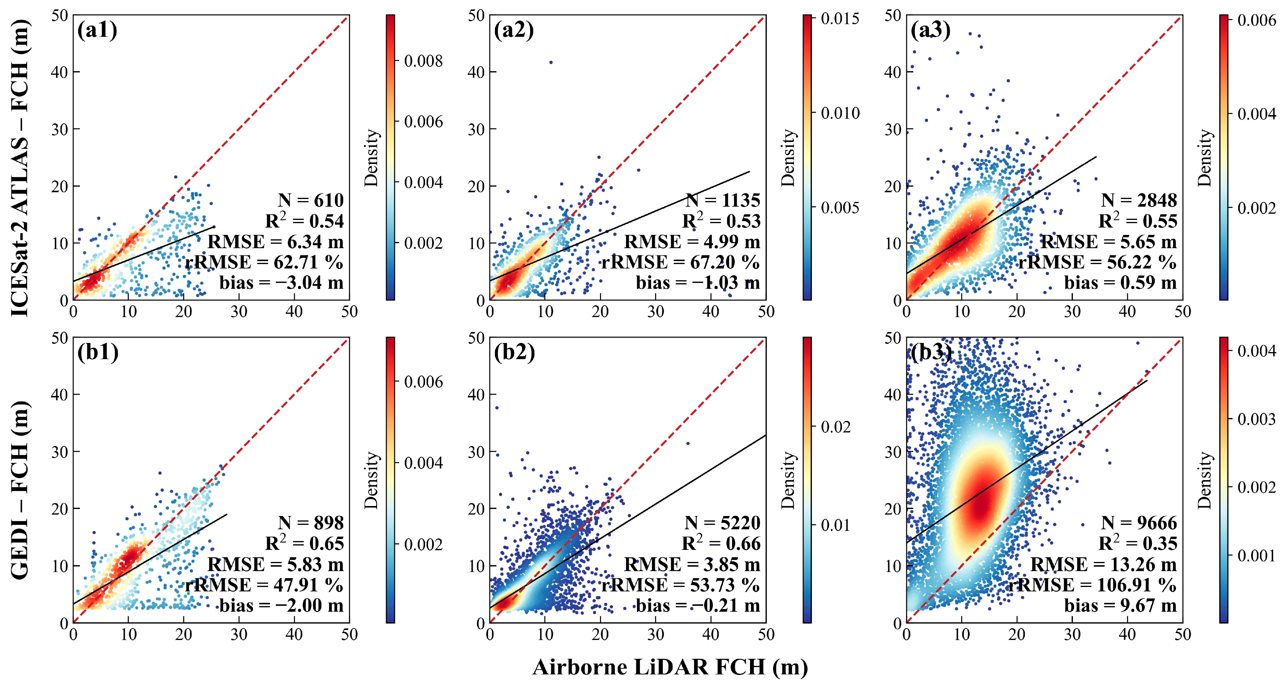
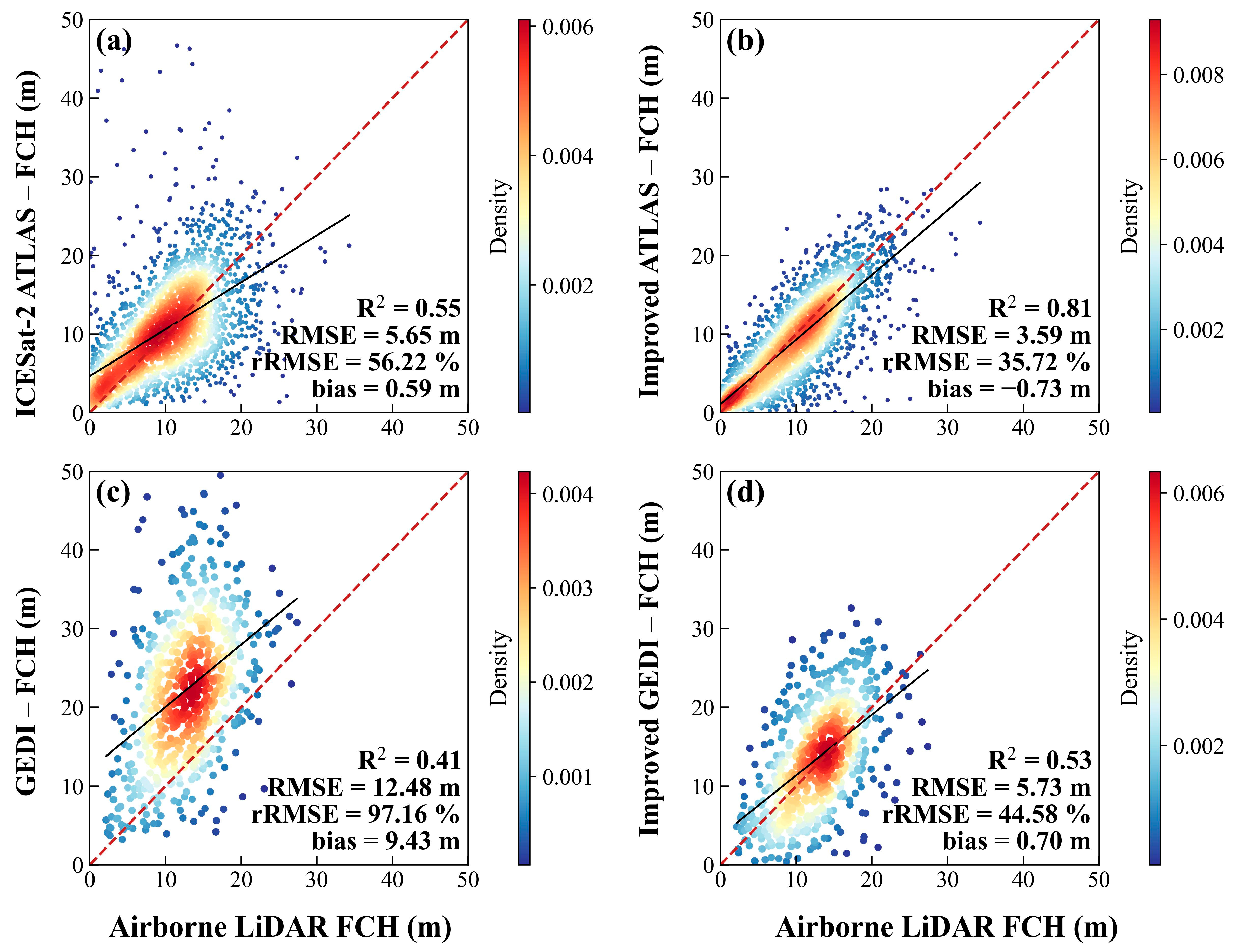
4.2. Evaluation of Forest Canopy Height Products from ICESat-2 ATLAS and GEDI

The comparison of FCHs from ATLAS and GEDI with ALS FCH across plain, hill, and mountain regions (Figure 5) revealed relatively poor accuracies. In both plain and hill regions, ATLAS FCH exhibited lower accuracy than GEDI FCH. The negative biases in FCH for plain and hilly regions suggest an underestimation of the true canopy height. In plain areas, due to sparse and scattered vegetation cover and positional errors in spaceborne LiDAR data, FCH in Lixin County had the highest underestimation, with biases of −3.04 m for ATLAS and −2.00 m for GEDI. In the mountain region, high outliers in ATLAS data resulted in a slight overestimation of FCH, with a bias of 0.59 m. However, GEDI FCH showed the largest error in the mountain region, with RMSE of 13.26 m and bias of 9.67 m, significantly higher than ATLAS, indicating a severe overestimation. Therefore, ATLAS FCH data were found to be more accurate than GEDI FCH data in mountain areas. Additionally, in all regions, the quantity of data from GEDI was much larger than that from ATLAS, especially in hill and mountain areas (the number of GEDI data was nearly 3 to 5 times larger than that of ATLAS).
The analysis of ATLAS-FCH and GEDI-FCH accuracies under varying terrain slopes and vegetation covers in mountain region (Huangshan district) (Figure 6) revealed that RMSE and bias of both ATLAS FCH and GEDI FCH increased with rising slopes. However, the rates of increase differed significantly. For ATLAS FCH, the RMSE and bias exhibited only slight changes until the slope reached 40°–50°. In contrast, the RMSE and bias of GEDI FCH started to increase rapidly after the slope exceeded 20°–30° (Figure 6(a1,b1)). This suggests that the accuracy of GEDI FCH is more sensitive to slope than that of ATLAS FCH.
Since the accuracies of both ATLAS FCH and GEDI FCH were not significantly affected by low slopes (as shown in Figure 6(a1,b1,c1)), footprints with slopes less than 20° were selected for analyzing the impact of vegetation cover on FCH retrieval accuracy to avoid interaction between slope and vegetation cover. Figure 6(a2,b2,c2) shows that the RMSE of ATLAS FCH was less affected by canopy cover, but rRMSE peaked at low canopy cover, and bias decreased as canopy cover increased, particularly at a high canopy cover level. For GEDI, both the RMSE and bias of FCH decreased with increasing vegetation cover, showing a significant reduction in rRMSE. The decreasing bias of both ATLAS and GEDI FCH with the increasing canopy cover implies that spaceborne LiDAR systems may detect understory vegetation rather than the ground under denser canopy cover conditions, resulting in higher ground elevation. For ATLAS, as canopy cover increases, more canopy photons were captured, leading to more precise canopy elevation and a slight reduction in RMSE.

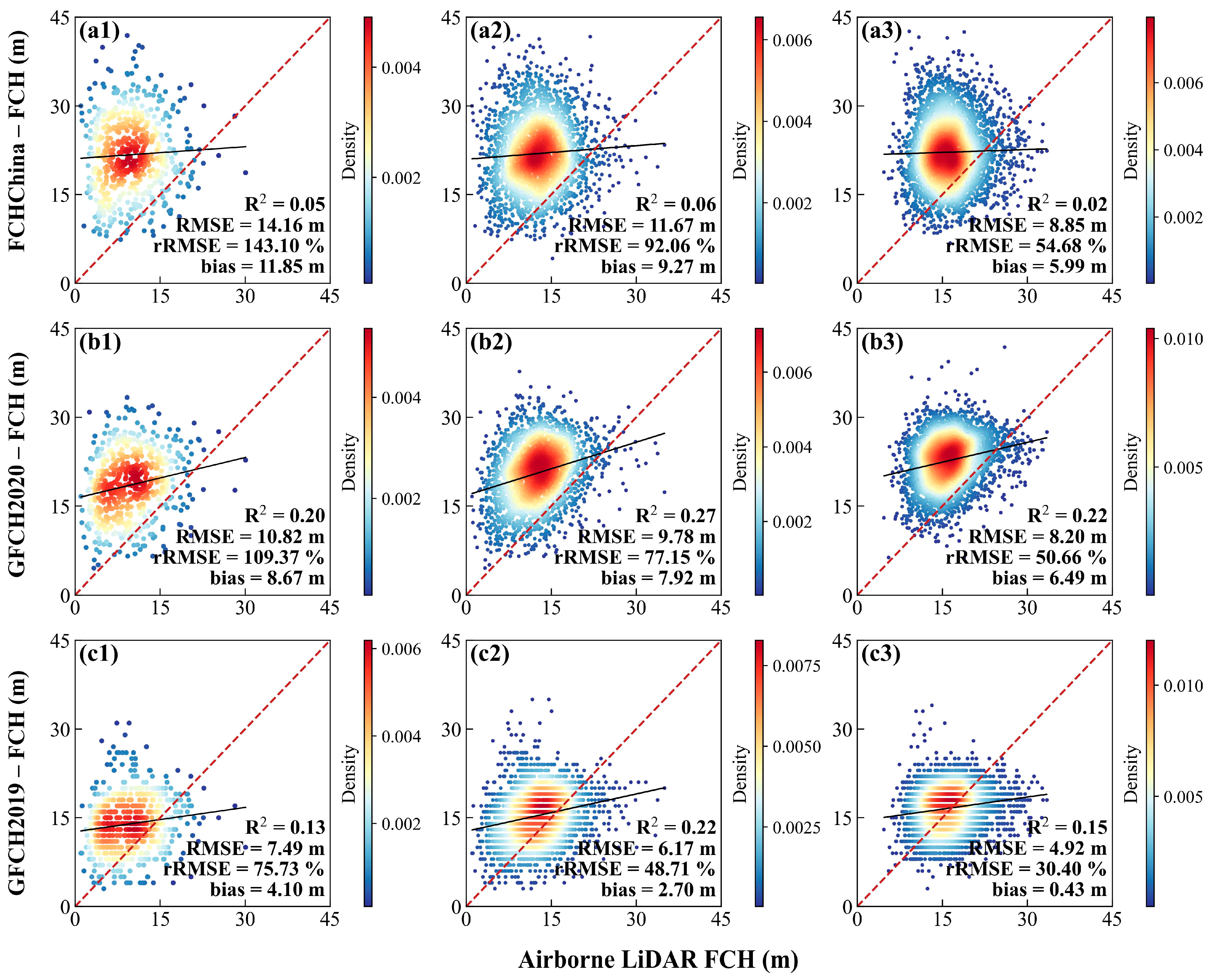
4.3. Evaluation of Three Wall-to-Wall FCH Products

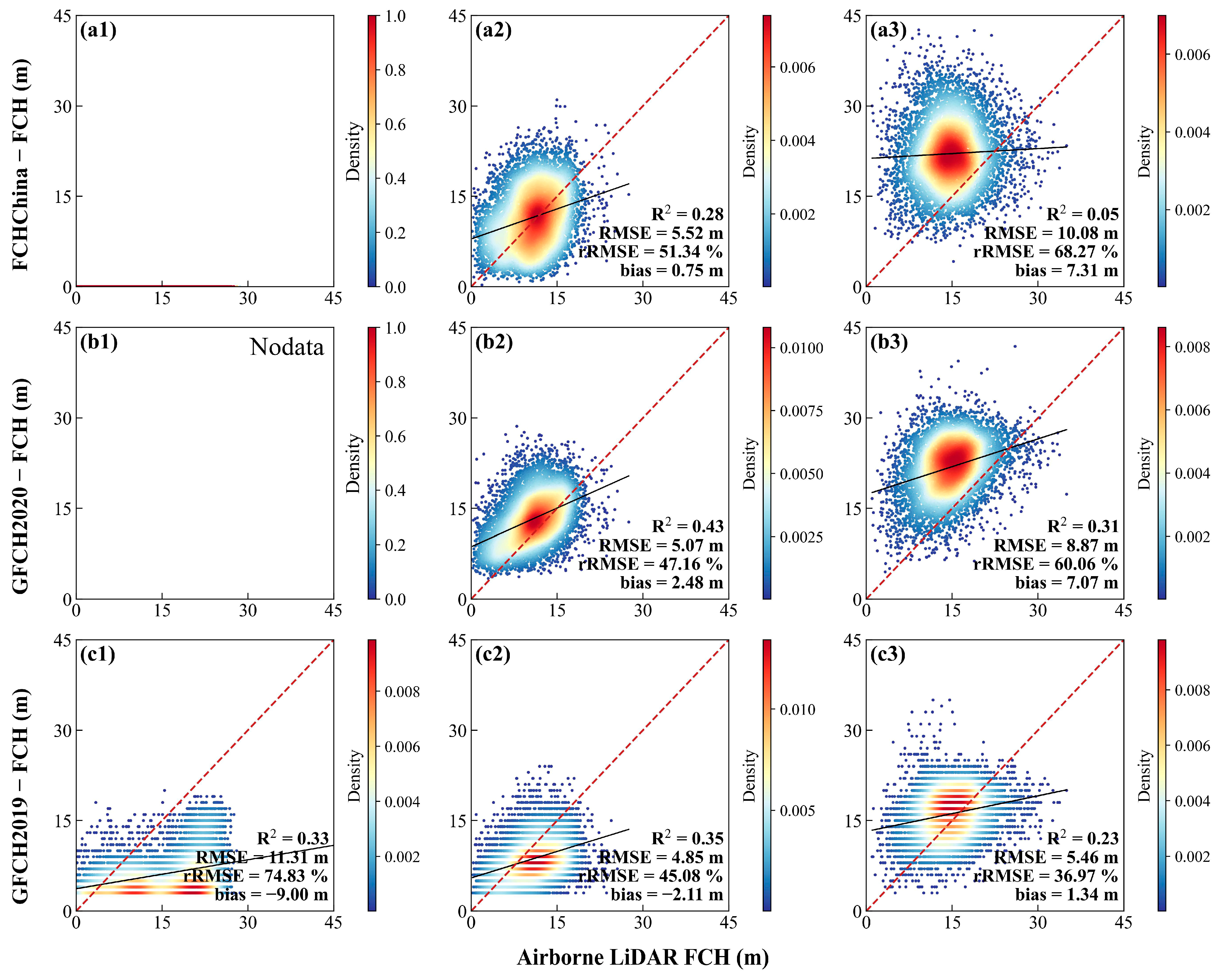
4.3.1. Evaluation of Wall-to-Wall FCH Products Based on Different Topographic Conditions

The relationship between three wall-to-wall FCH products and corresponding ALS FCHs, based on randomly selected 8000 pixels under different topographical conditions, (Figure 7) indicate that all three FCH products demonstrated reasonably good accuracies in the hilly region, but they performed relatively poorly in either mountainous or plain regions, as assessed by RMSE, rRMSE, and the availabilities of FCH values. In the hilly region, GFCH2019 exhibited the smallest RMSE (4.85 m) and rRMSE (45.01%) values, followed by GFCH2020 and FCHChina. Overall, GFCH2019 underestimated FCH by 2.11 m, GFCH2020 overestimated FCH by 2.48 m, and FCHChina slightly overestimated FCH by 0.75 m. In the mountainous region, GFCH2019 again had the lowest RMSE (5.46 m) and rRMSE (36.97%) compared to the other two products, slightly overestimating FCH by 1.34 m. In contrast, GFCH2020 and FCHChina exhibited higher RMSE and rRMSE values, and both significantly overestimated FCH by over 7 m. Interestingly, in the plain region, FCH values were absent in the FCHChina and GFCH2020 products due to the mask of non-vegetation areas (Figure 7(a1,b1)) but were present in GFCH2019, though its accuracy was poor, with an RMSE of 11.31 m and rRMSE of 74.83%. This poor performance may be attributed to the forest distribution patterns in Lixin County, where forests are sparsely scattered and narrowly striped along roads and rivers. The overall low accuracies of all three FCH products in the plain and mountainous regions highlight the challenges in accurately mapping FCH at large scales, even with global availability of spaceborne LiDAR systems such as ATLAS and GEDI.

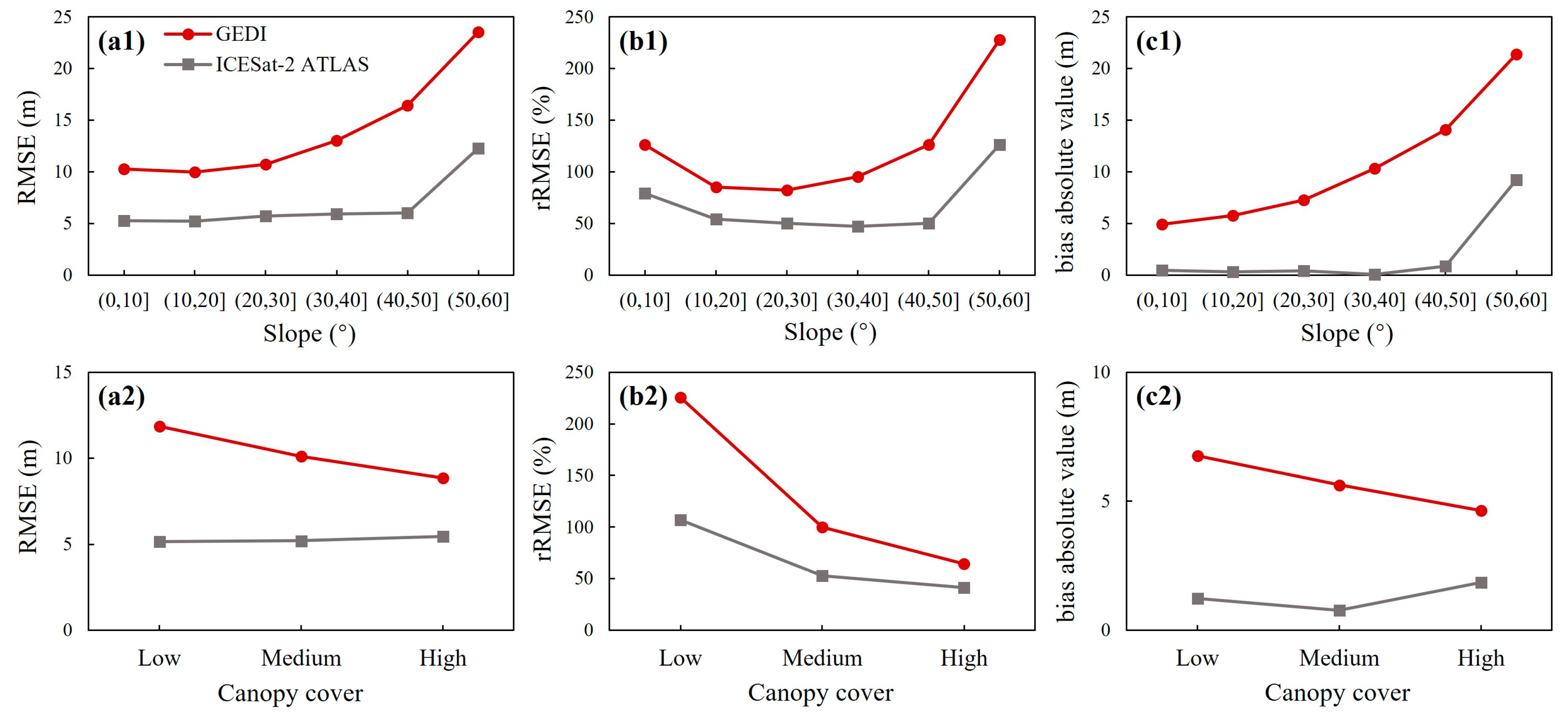
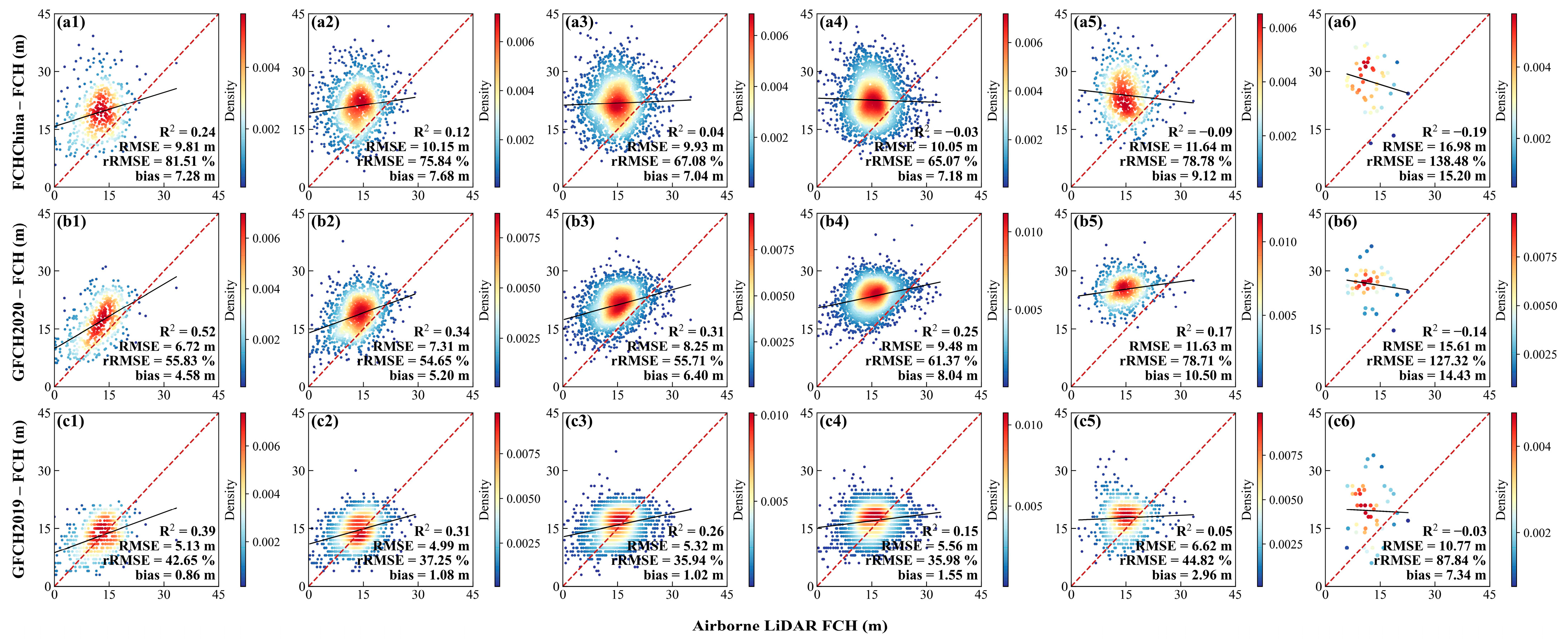
4.3.2. Evaluation of Wall-to-Wall FCH Products Based on Different Terrain Slopes

The wall-to-wall FCH products in mountainous regions were further analyzed using the ALS FCH data as reference. The residual changes with the slope levels (Figure 8) indicate that both FCHChina and GFCH2020 consistently overestimated FCH across all slopes. GFCH2019, however, showed close alignment with ALS FCH at lower slopes but gradually deviated, with positive residuals, as slopes increased. Specifically, for FCHChina, the mean residual remained relatively stable, around 7 m, until the slope exceeded 40°, after which FCH overestimation became extreme (the mean residual from 7.35 m to 8.46 m, until 17 m). Both GFCH2020 and GFCH2019 exhibited increasing mean residuals with the slope, though GFCH2019 showed a lower rate of residual change than GFCH2020. The accuracy assessment of the three products at different slopes (Figure 9) confirmed that FCHChina and GFCH2020 were more prone to overestimation than GFCH2019. All three products were influenced by terrain slopes, achieving the highest accuracy at low slopes (less than 20°), with the largest R2 and the lowest RMSE and bias values. Among the three, GFCH2019 had the smallest bias and RMSE. As the slope increased, the accuracy of FCH decreased for all products, but GFCH2019 still continued to outperform the others.

4.3.3. Evaluation of Wall-to-Wall FCH Products under Different Vegetation Characteristics

The accuracies of three FCH products in the mountainous region were further evaluated using ALS FCH, considering two key factors—forest types (i.e., Masson pine, Chinese fir, Moso bamboo, and broadleaf) and canopy cover levels (low, medium, and high). The analysis revealed RMSE values ranging from 4.28 m to 11.66 m, with the lowest RMSE observed in Moso bamboo and the highest in Masson pine (Figure 10). Among these products, GFCH2019 consistently outperformed FCHChina and GFCH2020 across all forest types, with the lowest RMSE, rRMSE, and bias values. When examining the accuracies of FCH products across different canopy cover levels (Figure 11), the results indicated that as canopy cover increased, both RMSE and bias values decreased. For example, GFCH2019’s RMSE, rRMSE, and bias values improved from 7.49 m, 75.73%, and 4.10 m at low canopy cover to 4.92 m, 30.40%, and 0.43 m at high canopy cover, respectively. Consistently, GFCH2019 provided the most accurate FCH estimations across all canopy cover levels compared to the other products.

4.4. Retrieval of FCHs through Incorporation of High-Quality DEM and Spaceborne LiDAR DSM

In the mountainous region, the quantity and quality of ATLAS ground photons are significantly influenced by terrain slope and vegetation cover. Dense vegetation cover and steep slopes often result in a limited number of ground photons, complicating generation of accurate DEMs. To address this issue, we utilized ALS DEM. By subtracting the mean value of the ALS DEM within the ATLAS footprint from the ATLAS canopy elevation, we derived spaceborne LiDAR FCH. This approach led to a significant improvement in FCH estimation accuracy compared to the original ATLAS canopy heights product, as evidenced by the reduced RMSE and increased R2 values (Figure 12b vs. Figure 12a). These results underscored the effectiveness of integrating accurate DEM and DSM data for filtering noisy photons and enhancing the precision of FCH estimations.
Conversely, the GEDI FCH product exhibited significant overestimation of FCH in mountainous regions (Figure 12c). On steep slopes, the GEDI ground waveform tends to stretch, causing the ground and vegetation returns to mix [39,40], making it challenging to identify the ground return in the GEDI waveform. To mitigate this issue, Wang et al. [39] proposed the GEDI-SAWA algorithm, which adjusted the GEDI waveform metrics based on the difference between the percentile metrics of the GEDI waveform and the corresponding metrics of the bare ground waveform, considering the terrain slope on the footprint. Utilizing this approach, we calculated the GEDI FCH in mountainous areas by subtracting the 98th percentile height of the ALS DEM from the GEDI canopy elevation. This adjustment reduced RMSE from 12.48 m to 5.73 m and decreased bias from 9.43 m to 0.70 m (Figure 12c vs. Figure 12d), indicating that incorporation of high quality ALS DEM can greatly enhance the accuracy of GEDI FCH in steep mountainous regions.

5. Discussion

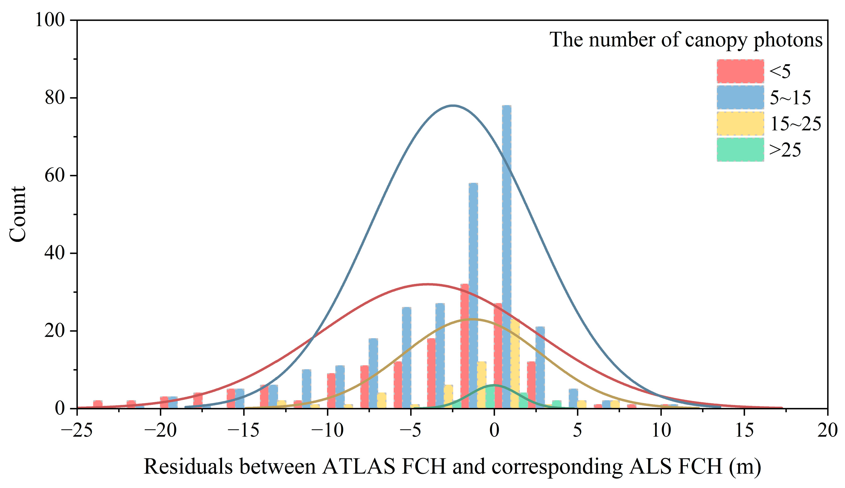
5.1. Factors Influencing FCH Retrieval from ATLAS Data

Many factors, including the misclassification of photon types and photon denoising and filtering methods, affect the accuracy of FCH retrieval from ATLAS data [41,42]. The moving overlapping window strategies and the cubic spine interpolation method used to identify ground and canopy photons after noise filtering during ATLAS data processing may overlook the impacts of topographic conditions and canopy coverage on photon quality, resulting in errors in FCH retrievals [43]. Figure 13 showed that acquiring more canopy photons would extract more accurate heights in plain regions, whereas acquiring and accurately classifying canopy photons under low vegetation cover conditions was challenging (Figure 3). That is a reason for the low accuracy of the current ATL08 FCH product in plain regions where forests are distributed in narrow and strip patterns. To address this issue, Wang et al. [44] proposed a sectional ATLAS photon-denoising method to reprocess ATLAS segments, reducing the RMSE and rRMSE from 5.13 m and 61.1% in the original ALT08 to 3.52 m and 31.1%, respectively, when compared with ALS data.
Some of the previous research assessed the accuracy of ATLAS FCH in forested regions. For instance, Liu et al. [25] evaluated the canopy height accuracy of ATL08 (version 4) for a 100 m segment and reported RMSE of 3.93 m (only strong beam data at night) and Moudrý et al. [27] reported 5.09 m in mountain area. Our research evaluated the FCH product of ATL08 (version 6) for a 20 m segment and found RMSE of 4.99 m in hill and 5.65 m in mountain regions. This may indicate the improvement of new version ATALS FCH products compared with the former versions.
In hilly regions, the canopy cover is generally higher than in plain regions, resulting in a less pronounced underestimation of FCH (Figure 5). As confirmed in this research, ATLAS FCH demonstrated higher accuracy in hilly regions than in plain or mountainous regions. However, the relatively steep terrain led to the overestimation of canopy photon heights. Therefore, appropriate photon denoising and filtering algorithms were crucial for FCH retrieval from ATLAS data in both plain and hilly regions, and sufficient canopy photons were a prerequisite for generating accurate and reliable FCH for ATLAS segments.
Mountainous regions are generally covered with large forest extents and have steep terrain. The dense vegetation cover makes it difficult for the ATLAS laser beam to reach the ground, while the steep terrain easily causes deviations in photon height. Thus, the lack of accurate ground elevation becomes a major problem for ATLAS to obtain accurate FCH in the mountainous region [45]. When terrain slopes are greater than 40°, FCH is more likely to be overestimated (Figure 6). Therefore, further denoising and filtering of canopy photons in the steep terrain of mountainous regions may improve the accuracy of ATLAS FCH products.

5.2. Factors Influencing FCH Retrieval from GEDI Data

GEDI products (Version 2) exhibit a geographic positioning error of approximately 10 m [46]. These geolocation errors in GEDI data have been identified as a significant factor impacting FCH accuracy, especially in spatially fragmented and heterogeneous canopy regions [47]. As shown in [44], geolocation errors in sparsely forested areas led to high FCH errors, with RMSE of 3.1 m and rRMSE of 27%. Their proposed correction method significantly improved the accuracy of GEDI FCH, reducing the RMSE to 2.3 m and the rRMSE to 18.4% in plain regions. Despite the influence of the geolocation error, GEDI FCH in plains and hilly regions still exhibited relatively high accuracy (Figure 4 and Figure 5), showing that GEDI had a greater capability for acquiring canopy heights than ATLAS in plain and hilly regions, particularly under high canopy cover and relatively flat terrain conditions. An interesting finding in this research was that the GEDI L2A product exhibited systematic biases in the extracted ground and canopy elevations from the received waveforms compared to ALS reference values (Figure 4). This implies that FCH can be effectively extracted in plain regions if geolocation errors are properly corrected.
The previous studies demonstrated that the accuracy of GEDI FCH retrieval was affected by slopes [25,28], with the RMSE of GEDI FCH increasing from around 3 m to 6 m as the slope rises [25]. In steep mountainous regions, such as the area of Huangshan district in this research, steep slopes considerably affected the GEDI FCH retrieval accuracy, and the GEDI data were more seriously affected by terrain than ATLAS; the RMSE of GEDI FHC has reached nearly 10 m at low slopes in our study. A slope greater than 20° led to a substantial increase in FCH retrieval error. This finding is consistent with the previous research that GEDI data should be used in forested regions with slopes less than approximately 30° [25], and this condition could be used as a threshold to filter for more reliable GEDI footprints [48,49]. Relatively homogeneous vegetation cover in mountainous regions can mitigate geolocation errors in GEDI measurements to a certain extent. While higher vegetation cover enhances the GEDI FCH retrieval accuracy, it does not significantly reduce the FCH errors induced by terrain characteristics. Minimizing topographic effects is the most critical factor in improving the retrieval accuracy of GEDI FCH in mountainous regions. Incorporating auxiliary data when processing GEDI waveforms to extract FCH is a typical approach to reduce the impact of terrain slope [50,51,52].

5.3. Factors Influencing Wall-to-Wall FCH Products from the Combination of ATLAS and/or GEDI and Other Data Sources

The previous validation indicated an RMSE of 4.93 m for FCHChina and 9.07 m for GFCH2019 [6,17]. This research showed that FCHChina had similar RMSE value in hilly areas, but had high RMSE in mountainous regions. The GFCH2019 product exhibited higher accuracy in both hilly and mountainous areas than FCHChina and GFCH2020. The RMSE of 9.07 m for GFCH2019 may be attributed to the substantial errors associated with FCH in plain areas (where our study found the RMSE of 11.31 m).
The development of wall-to-wall FCH products often involves integrating ATLAS and/or GEDI data with other remotely sensed data such as Landsat or Sentinel-2 [6,17]. Most wall-to-wall FCH products have focused on forested areas in mountainous regions with little attention to plain areas. This may be due to the sparse forest distribution and the limited proportion of forest areas in plains. The visual examination of three FCH products revealed that they failed to provide accurate FCH estimates in plain areas where the forests were sparsely distributed. In contrast, a quantitative assessment indicated that FCH estimates were most accurate in hilly regions. However, estimation errors sharply increased in mountainous regions due to the complex terrain condition. In wall-to-wall FCH estimation, a significant portion of the errors arose from the inherent inaccuracies of spaceborne LiDAR products. As confirmed in this research, both ATLAS and GEDI FCH products exhibited certain errors due to factors such as the characteristics of LiDAR systems, topography, and vegetation conditions. When used as input for wall-to-wall FCH estimation, these errors propagated into the final output. Other factors that may impact the accuracy of the wall-to-wall FCH product included vegetation cover, forest type, forest map accuracy, and the methods used for estimation.
The analysis of FCH products in mountainous areas indicated that vegetation cover significantly impacted the accuracy of all three wall-to-wall products, with the highest FCH accuracy observed in areas with medium vegetation cover. In regions with low vegetation cover, the presence of bare soils greatly affected the spectral reflectance of optical sensors and introduced uncertainty in both ATLAS and GEDI FCH estimation. Conversely, in densely vegetated regions, signal saturation in optical and SAR data [53] led to an underestimation of tall trees. Potapov et al. [17] noted that their model, which utilized Landsat analysis-ready time-series data, saturated above 30 m.
FCH estimation accuracies also varied among forest types. Masson pine, a pioneer species often mixed with other understory species in harsh environment, presented challenges for accurate FCH estimation due to its complex forest stand structure and terrain conditions. Optical or SAR data struggled to accurately characterize the FCH in these conditions, it may result in poor FCH estimation. In contrast, Moso bamboo forests, with their more uniform canopy height and homogeneous stand structures, achieved the highest FCH estimation accuracy among four forest types across all three wall-to-wall FCH products.
A high-quality and detailed forest distribution map is essential for accurate FCH mapping. Firstly, forest distribution maps are often used for a reference to mask other land cover types, leaving only forested areas for further FCH estimation and analysis. Secondly, forest types impact the accuracy of FCH estimates from both spaceborne LiDAR at segments and footprints and wall-to-wall at the pixel level, as demonstrated in this research. Thus, the accuracy of general forest distribution and forest type classification is crucial for FCH estimation. The forest map data used in three wall-to-wall products examined in this research varied in terms of data sources and accuracies, but all had some issues. FCHChina [6] used the Globaland30 land cover product from 2015 to extract forest areas, while GFCH2020 [35] relied on the GLC_FC30 land cover product from 2020, grouping forests into five types: evergreen broadleaved, deciduous broadleaved, mixed-leaf forest, evergreen needle-leaved, and deciduous needle-leaved. Both forest datasets were coarse in forest classification and did not adequately consider variations between forest types, and the Globaland30 product was outdated compared to other datasets in the study. GFCH2019 [17] did not differentiate forests from other land cover types, leading to confusion between tree height and building height in urban and suburban areas.
Appropriate algorithms are also important for wall-to-wall FCH estimation. The three wall-to-wall FCH products assessed in this research provided promising approaches to regional scale FCH mapping, including a neural-network-guided interpolation method [6], random forest, or regression tree ensemble algorithm [17,35]. The random forest method has advantages in processing multi-sources data at large scales and is widely used in classification and regression. However, the uneven distribution of tree height samples can lead to overestimation of low values or underestimation of high values when inferring from spaceborne LiDAR footprint scale to regional scale. Additionally, with an imbalanced sample distribution, the random forest algorithm may exhibit a tendency to overfit predictions, highlighting the importance of representative sample datasets. The spatial distribution of datasets is equally important [54]. Lang et al. [11] developed a convolutional neural network (CNN) deep learning method for mapping regional and global canopy heights, which greatly reduced the errors related to underestimation of tall trees. However, even though spaceborne LiDAR can capture canopy heights of relatively low vegetation, most current wall-to-wall FCH products still suffered from a widespread overestimation of low values.

5.4. Potential Solutions for Improving FCH Retrieval Performance

The evaluation of ATLAS and GEDI FCH highlights the significant impact of topographic and canopy cover condition on FCH accuracy, underscoring the need to develop appropriate methods that account for these factors when processing ATLAS and GEDI data. In sparsely forested areas, such as plain regions and some hilly regions, it is critical to develop advanced algorithms that improve the separation of canopy photons from noise in ATLAS data, given the insufficient number of canopy photons to accurately represent the canopy surface. Additionally, enhancing geolocation accuracy in GEDI data is essential in these regions. In mountainous regions, ATLAS data face the challenge of a lack of ground photons due to dense canopy cover, while GEDI data are impacted by both steep slopes and dense canopy cover [39,55]. As a result, extracting FCH in densely forested regions is difficult using either ATLAS or GEDI. Incorporating high-precision DEM data derived from ALS into processing ATLAS or GEDI data may improve spaceborne LiDAR-derived FCH [45]. Further research is needed to develop methods to supplement or improve the detection of missing ground photons in ATLAS segment, as well as approaches to mitigate waveform broadening issues in GEDI.
To improve wall-to-wall FCH products derived from the integration of spaceborne LiDAR FCH data and other remotely sensed data (e.g., Landsat, Sentinel-1/2), the most direct approach is to utilize improved spaceborne LiDAR FCH products as input. This can be achieved by developing new algorithms. For example, Huang et al. [56] proposed an adaptive filter called “Threshold Segmentation based on Spatial Clustering and Bimodal Reconstruction (TS-SCABR)”, which, combined with the gradient method, effectively identified ground and non-ground photons and refined the classification of photon types. This approach significantly improved FCH accuracy under various natural conditions compared to the original ATL08 product, particularly in scenarios with low vegetation cover and steep slopes in mountainous areas. Secondly, making full use of the spectral and spatial features of optical and SAR data, along with ancillary data helped reduce the saturation problem. The research has shown that incorporating textural information from optical data into CNN models or other models effectively mitigated the saturation of tall canopies [11,57]. High-quality forest type distribution data and appropriate methods are also crucial for improving FCH estimation. Further research is needed to explore the effective use of multi-source data and to develop suitable methods for enhancing FCH products.

6. Conclusions

This research evaluated the accuracy of ATLAS and GEDI FCH products, as well as three wall-to-wall FCH products (FCHChina, GFCH2020, and GFCH2019) using ALS FCH as a reference. The study also analyzed the impact of landforms, slopes, and vegetation characteristics on accuracy. For ATLAS and GEDI FCH, the results indicate that: (1) GEDI FCH is more accurate in plain and hilly regions but is significantly affected by slope in mountainous region, leading to reduced accuracy. In contrast, ATLAS FCH is more accurate in mountainous areas and less accurate in plains and hilly regions with relatively sparse vegetation cover; (2) Slopes exceeding a certain degree lead to substantial errors in both ATLAS and GEDI FCH: slope > 40° for ATLAS and slope > 20° for GEDI in mountainous region; (3) Both ATLAS and GEDI FCH exhibit the highest accuracy (the smallest rRMSE) in areas with high canopy cover.
For wall-to-wall FCH products, the following conclusions were drawn: (1) All three FCH products exhibited higher accuracy in the hilly region than in plain and mountainous regions; (2) GFCH2019 estimates were the most accurate, overall, but it underestimated FCH in the plain and hill regions. FCHChina and GFCH2020 greatly overestimated FCH in the mountainous region; (3) The accuracy of FCH was significantly affected by slope and vegetation cover. As slope increased, FCH errors increased. FCH was prone to overestimation in areas with low canopy cover; (4) FCH accuracy varied among different forest types, with the FCH of Moso bamboo forests being the most accurate and that of Masson pine forests being the least accurate, possibly due to differences in forest stand structure.
Improving the accuracy of spaceborne LiDAR FCH by developing more advanced algorithms to process ATLAS photons and GEDI waveforms is necessary when combining these data with other data sources for wall-to-wall FCH estimation at a large scale. In addition to enhancing FCH retrieval accuracy from ATLAS and GEDI data, more research is needed to effectively integrate different data sources in wall-to-wall FCH mapping. This includes improving estimation by mitigating data saturation problems in optical and SAR data, collecting representative sample datasets, and developing more advanced modeling methods.

Author Contributions

Conceptualization, D.L. (Dengsheng Lu) and G.L. (Guiying Li); methodology, Y.L. (Yisa Li); software, Y.L. (Yisa Li); validation, Y.L. (Yisa Li) and Y.L. (Yagang Lu); formal analysis, Y.L. (Yisa Li); investigation, Y.L. (Yisa Li) and Y.L. (Yagang Lu); resources, Y.L. (Yisa Li) and Y.L. (Yagang Lu); data curation, Y.L. (Yisa Li) and Y.L. (Yagang Lu); writing—original draft preparation, Y.L. (Yisa Li) and D.L.; writing—review and editing, D.L., Y.L. (Yagang Lu), and G.L.; visualization, Y.L. (Yisa Li) and D.L.; supervision, D.L. and G.L.; project administration, D.L. and G.L.; funding acquisition, D.L. and G.L. All authors have read and agreed to the published version of the manuscript.

Funding

This research was funded by the National Natural Science Foundation of China, grant number #32171787 and National Key R&D Program of China, grant number 2021YFD2200400102.

Data Availability Statement

The ICESat-2 ATLAS, GEDI, and DEM data are publicly available, and airborne LiDAR data are not publicly available due to confidentiality agreements.

Acknowledgments

The authors would like to thank Ruoqi Wang for her help during the data processing.

Conflicts of Interest

The authors declare no conflicts of interest. The funders had no role in the design of the study; in the collection, analyses, or interpretation of data; in the writing of the manuscript; or in the decision to publish the results.

References

  1. Fischer, R.; Knapp, N.; Bohn, F.; Shugart, H.H.; Huth, A. The Relevance of Forest Structure for Biomass and Productivity in Temperate Forests: New Perspectives for Remote Sensing. Surv. Geophys. 2019, 40, 709–734. [Google Scholar] [CrossRef]
  2. Lefsky, M.A.; Harding, D.J.; Keller, M.; Cohen, W.B.; Carabajal, C.C.; Del Bom Espirito-Santo, F.; Hunter, M.O.; De Oliveira, R. Estimates of forest canopy height and aboveground biomass using ICESat. Geophys. Res. Lett. 2005, 32, 2005GL023971. [Google Scholar] [CrossRef]
  3. Patenaude, G.; Hill, R.A.; Milne, R.; Gaveau, D.L.A.; Briggs, B.B.J.; Dawson, T.P. Quantifying forest above ground carbon content using LiDAR remote sensing. Remote Sens. Environ. 2004, 93, 368–380. [Google Scholar] [CrossRef]
  4. Liao, K.; Li, Y.; Zou, B.; Li, D.; Lu, D. Examining the Role of UAV Lidar Data in Improving Tree Volume Calculation Accuracy. Remote Sens. 2022, 14, 4410. [Google Scholar] [CrossRef]
  5. Lu, D.; Jiang, X. A brief overview and perspective of using airborne Lidar data for forest biomass estimation. Int. J. Image Data Fusion 2024, 15, 1–24. [Google Scholar] [CrossRef]
  6. Liu, X.; Su, Y.; Hu, T.; Yang, Q.; Liu, B.; Deng, Y.; Tang, H.; Tang, Z.; Fang, J.; Guo, Q. Neural network guided interpolation for mapping canopy height of China’s forests by integrating GEDI and ICESat-2 data. Remote Sens. Environ. 2022, 269, 112844. [Google Scholar] [CrossRef]
  7. Tamiminia, H.; Salehi, B.; Mahdianpari, M.; Goulden, T. State-wide forest canopy height and aboveground biomass map for New York with 10 m resolution, integrating GEDI, Sentinel-1, and Sentinel-2 data. Ecol. Inform. 2024, 79, 102404. [Google Scholar] [CrossRef]
  8. Travers-Smith, H.; Coops, N.C.; Mulverhill, C.; Wulder, M.A.; Ignace, D.; Lantz, T.C. Mapping vegetation height and identifying the northern forest limit across Canada using ICESat-2, Landsat time series and topographic data. Remote Sens. Environ. 2024, 305, 114097. [Google Scholar] [CrossRef]
  9. Neumann, T.A.; Martino, A.J.; Markus, T.; Bae, S.; Bock, M.R.; Brenner, A.C.; Brunt, K.M.; Cavanaugh, J.; Fernandes, S.T.; Hancock, D.W.; et al. The Ice, Cloud, and Land Elevation Satellite—2 mission: A global geolocated photon product derived from the Advanced Topographic Laser Altimeter System. Remote Sens. Environ. 2019, 233, 111325. [Google Scholar] [CrossRef]
  10. Dubayah, R.; Blair, J.B.; Goetz, S.; Fatoyinbo, L.; Hansen, M.; Healey, S.; Hofton, M.; Hurtt, G.; Kellner, J.; Luthcke, S.; et al. The Global Ecosystem Dynamics Investigation: High-resolution laser ranging of the Earth’s forests and topography. Sci. Remote Sens. 2020, 1, 100002. [Google Scholar] [CrossRef]
  11. Lang, N.; Jetz, W.; Schindler, K.; Wegner, J.D. A high-resolution canopy height model of the Earth. Nat. Ecol. Evol. 2023, 7, 1778–1789. [Google Scholar] [CrossRef] [PubMed]
  12. Zhang, Z.; Ni, W.; Quegan, S.; Chen, J.; Gong, P.; Rodriguez, L.C.E.; Guo, H.; Shi, J.; Liu, L.; Li, Z.; et al. Deforestation in Latin America in the 2000s predominantly occurred outside of typical mature forests. Innovation 2024, 5, 100610. [Google Scholar] [CrossRef] [PubMed]
  13. Wu, Z.; Shi, F. Mapping Forest Canopy Height at Large Scales Using ICESat-2 and Landsat: An Ecological Zoning Random Forest Approach. IEEE Trans. Geosci. Remote Sens. 2022, 61, 1–16. [Google Scholar] [CrossRef]
  14. Schwartz, M.; Ciais, P.; De Truchis, A.; Chave, J.; Ottlé, C.; Vega, C.; Wigneron, J.-P.; Nicolas, M.; Jouaber, S.; Liu, S.; et al. FORMS: Forest Multiple Source height, wood volume, and biomass maps in France at 10 to 30 m resolution based on Sentinel-1, Sentinel-2, and GEDI data with a deep learning approach. Earth Syst. Sci. Data 2023, 15, 4927–4945. [Google Scholar] [CrossRef]
  15. Li, W.; Niu, Z.; Shang, R.; Qin, Y.; Wang, L.; Chen, H. High-resolution mapping of forest canopy height using machine learning by coupling ICESat-2 LiDAR with Sentinel-1, Sentinel-2 and Landsat-8 data. Int. J. Appl. Earth Obs. Geoinf. 2020, 92, 102163. [Google Scholar] [CrossRef]
  16. Jiang, F.; Zhao, F.; Ma, K.; Li, D.; Sun, H. Mapping the Forest Canopy Height in Northern China by Synergizing ICESat-2 with Sentinel-2 Using a Stacking Algorithm. Remote Sens. 2021, 13, 1535. [Google Scholar] [CrossRef]
  17. Potapov, P.; Li, X.; Hernandez-Serna, A.; Tyukavina, A.; Hansen, M.C.; Kommareddy, A.; Pickens, A.; Turubanova, S.; Tang, H.; Silva, C.E.; et al. Mapping global forest canopy height through integration of GEDI and Landsat data. Remote Sens. Environ. 2021, 253, 112165. [Google Scholar] [CrossRef]
  18. Hancock, S.; Armston, J.; Hofton, M.; Sun, X.; Tang, H.; Duncanson, L.I.; Kellner, J.R.; Dubayah, R. The GEDI Simulator: A Large-Footprint Waveform Lidar Simulator for Calibration and Validation of Spaceborne Missions. Earth Space Sci. 2019, 6, 294–310. [Google Scholar] [CrossRef]
  19. Neuenschwander, A.; Magruder, L. The Potential Impact of Vertical Sampling Uncertainty on ICESat-2/ATLAS Terrain and Canopy Height Retrievals for Multiple Ecosystems. Remote Sens. 2016, 8, 1039. [Google Scholar] [CrossRef]
  20. Neuenschwander, A.; Guenther, E.; White, J.C.; Duncanson, L.; Montesano, P. Validation of ICESat-2 terrain and canopy heights in boreal forests. Remote Sens. Environ. 2020, 251, 112110. [Google Scholar] [CrossRef]
  21. Adam, M.; Urbazaev, M.; Dubois, C.; Schmullius, C. Accuracy Assessment of GEDI Terrain Elevation and Canopy Height Estimates in European Temperate Forests: Influence of Environmental and Acquisition Parameters. Remote Sens. 2020, 12, 3948. [Google Scholar] [CrossRef]
  22. Urbazaev, M.; Hess, L.L.; Hancock, S.; Sato, L.Y.; Ometto, J.P.; Thiel, C.; Dubois, C.; Heckel, K.; Urban, M.; Adam, M.; et al. Assessment of terrain elevation estimates from ICESat-2 and GEDI spaceborne LiDAR missions across different land cover and forest types. Sci. Remote Sens. 2022, 6, 100067. [Google Scholar] [CrossRef]
  23. Feng, T.; Duncanson, L.; Montesano, P.; Hancock, S.; Minor, D.; Guenther, E.; Neuenschwander, A. A systematic evaluation of multi-resolution ICESat-2 ATL08 terrain and canopy heights in boreal forests. Remote Sens. Environ. 2023, 291, 113570. [Google Scholar] [CrossRef]
  24. Li, H.; Li, X.; Kato, T.; Hayashi, M.; Fu, J.; Hiroshima, T. Accuracy assessment of GEDI terrain elevation, canopy height, and aboveground biomass density estimates in Japanese artificial forests. Sci. Remote Sens. 2024, 10, 100144. [Google Scholar] [CrossRef]
  25. Liu, A.; Cheng, X.; Chen, Z. Performance evaluation of GEDI and ICESat-2 laser altimeter data for terrain and canopy height retrievals. Remote Sens. Environ. 2021, 264, 112571. [Google Scholar] [CrossRef]
  26. Malambo, L.; Popescu, S.C. Assessing the agreement of ICESat-2 terrain and canopy height with airborne lidar over US ecozones. Remote Sens. Environ. 2021, 266, 112711. [Google Scholar] [CrossRef]
  27. Moudrý, V.; Gdulová, K.; Gábor, L.; Šárovcová, E.; Barták, V.; Leroy, F.; Špatenková, O.; Rocchini, D.; Prošek, J. Effects of environmental conditions on ICESat-2 terrain and canopy heights retrievals in Central European mountains. Remote Sens. Environ. 2022, 279, 113112. [Google Scholar] [CrossRef]
  28. Zhu, X.; Nie, S.; Zhu, Y.; Chen, Y.; Yang, B.; Li, W. Evaluation and Comparison of ICESat-2 and GEDI Data for Terrain and Canopy Height Retrievals in Short-Stature Vegetation. Remote Sens. 2023, 15, 4969. [Google Scholar] [CrossRef]
  29. Zhu, X.; Nie, S.; Wang, C.; Xi, X.; Lao, J.; Li, D. Consistency analysis of forest height retrievals between GEDI and ICESat-2. Remote Sens. Environ. 2022, 281, 113244. [Google Scholar] [CrossRef]
  30. Dong, J.; Ni, W.; Zhang, Z.; Sun, G. Performance of ICESat-2 ATL08 product on the estimation of forest height by referencing to small footprint LiDAR data. Natl. Remote Sens. Bull. 2021, 25, 1294–1307. [Google Scholar] [CrossRef]
  31. Fayad, I.; Ienco, D.; Baghdadi, N.; Gaetano, R.; Alvares, C.A.; Stape, J.L.; Ferraço Scolforo, H.; Le Maire, G. A CNN-based approach for the estimation of canopy heights and wood volume from GEDI waveforms. Remote Sens. Environ. 2021, 265, 112652. [Google Scholar] [CrossRef]
  32. Lahssini, K.; Baghdadi, N.; le Maire, G.; Fayad, I. Influence of GEDI acquisition and processing parameters on canopy height estimates over tropical forests. Remote Sens. 2022, 14, 6264. [Google Scholar] [CrossRef]
  33. Fayad, I.; Baghdadi, N.; Lahssini, K. An Assessment of the GEDI Lasers’ Capabilities in Detecting Canopy Tops and Their Penetration in a Densely Vegetated, Tropical Area. Remote Sens. 2022, 14, 2969. [Google Scholar] [CrossRef]
  34. Fayad, I.; Baghdadi, N.; Alcarde Alvares, C.; Stape, J.L.; Bailly, J.S.; Scolforo, H.F.; Cegatta, I.R.; Zribi, M.; Le Maire, G. Terrain Slope Effect on Forest Height and Wood Volume Estimation from GEDI Data. Remote Sens. 2021, 13, 2136. [Google Scholar] [CrossRef]
  35. Nie, S.; Zhu, X.; Wang, C.; Xi, X. The Global 30-m Forest Canopy Height Map for 2020; Version 1; Zenodo: Prévessin-Moëns, France, 2023. [Google Scholar] [CrossRef]
  36. Xing, Y.; Huang, J.; Gruen, A.; Qin, L. Assessing the Performance of ICESat-2/ATLAS Multi-Channel Photon Data for Estimating Ground Topography in Forested Terrain. Remote Sens. 2020, 12, 2084. [Google Scholar] [CrossRef]
  37. Lang, N.; Kalischek, N.; Armston, J.; Schindler, K.; Dubayah, R.; Wegner, J.D. Global canopy height regression and uncertainty estimation from GEDI LIDAR waveforms with deep ensembles. Remote Sens. Environ. 2022, 268, 112760. [Google Scholar] [CrossRef]
  38. Meadows, M.; Jones, S.; Reinke, K. Vertical accuracy assessment of freely available global DEMs (FABDEM, Copernicus DEM, NASADEM, AW3D30 and SRTM) in flood-prone environments. Int. J. Digit. Earth 2024, 17, 2308734. [Google Scholar] [CrossRef]
  39. Wang, Y.; Ni, W.; Sun, G.; Chi, H.; Zhang, Z.; Guo, Z. Slope-adaptive waveform metrics of large footprint lidar for estimation of forest aboveground biomass. Remote Sens. Environ. 2019, 224, 386–400. [Google Scholar] [CrossRef]
  40. Yang, W.; Ni-Meister, W.; Lee, S. Assessment of the impacts of surface topography, off-nadir pointing and vegetation structure on vegetation lidar waveforms using an extended geometric optical and radiative transfer model. Remote Sens. Environ. 2011, 115, 2810–2822. [Google Scholar] [CrossRef]
  41. Kui, M.; Xu, Y.; Wang, J.; Cheng, F. Research on the Adaptability of Typical Denoising Algorithms Based on ICESat-2 Data. Remote Sens. 2023, 15, 3884. [Google Scholar] [CrossRef]
  42. Chang, B.; Xiong, H.; Li, Y.; Pan, D.; Cui, X.; Zhang, W. ALCSF: An adaptive and anti-noise filtering method for extracting ground and top of canopy from ICESat-2 LiDAR data along single tracks. ISPRS J. Photogramm. Remote Sens. 2024, 215, 80–98. [Google Scholar] [CrossRef]
  43. Popescu, S.C.; Zhou, T.; Nelson, R.; Neuenschwander, A.; Sheridan, R.; Narine, L.; Walsh, K.M. Photon counting LiDAR: An adaptive ground and canopy height retrieval algorithm for ICESat-2 data. Remote Sens. Environ. 2018, 208, 154–170. [Google Scholar] [CrossRef]
  44. Wang, R.; Lu, Y.; Lu, D.; Li, G. Improving extraction of forest canopy height through reprocessing ICESat-2 ATLAS and GEDI data in sparsely forested plain regions. GISci. Remote Sens. 2024, 61, 2396807. [Google Scholar] [CrossRef]
  45. Pang, S.; Li, G.; Jiang, X.; Chen, Y.; Lu, Y.; Lu, D. Retrieval of forest canopy height in a mountainous region with ICESat-2 ATLAS. For. Ecosyst. 2022, 9, 100046. [Google Scholar] [CrossRef]
  46. Tang, H.; Stoker, J.; Luthcke, S.; Armston, J.; Lee, K.; Blair, B.; Hofton, M. Evaluating and mitigating the impact of systematic geolocation error on canopy height measurement performance of GEDI. Remote Sens. Environ. 2023, 291, 113571. [Google Scholar] [CrossRef]
  47. Roy, D.P.; Kashongwe, H.B.; Armston, J. The impact of geolocation uncertainty on GEDI tropical forest canopy height estimation and change monitoring. Sci. Remote Sens. 2021, 4, 100024. [Google Scholar] [CrossRef]
  48. Shendryk, Y. Fusing GEDI with earth observation data for large area aboveground biomass mapping. Int. J. Appl. Earth Obs. Geoinf. 2022, 115, 103108. [Google Scholar] [CrossRef]
  49. Aragoneses, E.; García, M.; Ruiz-Benito, P.; Chuvieco, E. Mapping forest canopy fuel parameters at European scale using spaceborne LiDAR and satellite data. Remote Sens. Environ. 2024, 303, 114005. [Google Scholar] [CrossRef]
  50. Allouis, T.; Durrieu, S.; Couteron, P. A New Method for Incorporating Hillslope Effects to Improve Canopy-Height Estimates from Large-Footprint LIDAR Waveforms. IEEE Geosci. Remote Sens. Lett. 2012, 9, 730–734. [Google Scholar] [CrossRef]
  51. Tang, H.; Huang, H.; Zheng, Y.; Qin, P.; Xu, Y.; Ding, S. Improved GEDI Canopy Height Extraction Based on a Simulated Ground Echo in Topographically Undulating Areas. IEEE Trans. Geosci. Remote Sens. 2023, 61, 1–15. [Google Scholar] [CrossRef]
  52. Zhou, H.; Wang, H.; Song, H.; Zhang, Q.; Ma, Y.; Li, S. Canopy Height Extraction Over Mountainous Areas from GEDI Lidar Deconvoluted Waveforms. IEEE Geosci. Remote Sens. Lett. 2024, 21, 1–5. [Google Scholar] [CrossRef]
  53. Mutanga, O.; Masenyama, A.; Sibanda, M. Spectral saturation in the remote sensing of high-density vegetation traits: A systematic review of progress, challenges, and prospects. ISPRS J. Photogramm. Remote Sens. 2023, 198, 297–309. [Google Scholar] [CrossRef]
  54. Baban, G.; Daniel Niţă, M. Measuring forest height from space. Opportunities and limitations observed in natural forests. Measurement 2023, 211, 112593. [Google Scholar] [CrossRef]
  55. Tian, X.; Shan, J. Detection of Signal and Ground Photons from ICESat-2 ATL03 Data. IEEE Trans. Geosci. Remote Sens. 2023, 61, 1–14. [Google Scholar] [CrossRef]
  56. Huang, X.; Cheng, F.; Wang, J.; Duan, P.; Wang, J. Forest Canopy Height Extraction Method Based on ICESat-2/ATLAS Data. IEEE Trans. Geosci. Remote Sens. 2023, 61, 1–14. [Google Scholar] [CrossRef]
  57. Lang, N.; Schindler, K.; Wegner, J.D. Country-wide high-resolution vegetation height mapping with Sentinel-2. Remote Sens. Environ. 2019, 233, 111347. [Google Scholar] [CrossRef]
Figure 1. The selected three study areas in Anhui Province: (a) Landform types; (b) Lixin County in plain region; (c) Lujiang County in hilly region; (d) Huangshan District in mountainous region, overlaid with ATLAS and GEDI tracks.
Remotesensing 16 03650 g001
Figure 2. Profiles of spaceborne LiDAR data and corresponding ALS data along the tracks in mountainous region (a) ICESat-2 ATLAS, (b) GEDI.
Remotesensing 16 03650 g002
Figure 3. Comparison of ATLAS photons and ALS DSM and DEM among plain, hill, and mountain with different slopes and canopy cover levels. (a1a4) different canopy levels in plain region; (b1b4) different combinations of slopes and canopy covers in hilly region; (c1c4) different combinations of slopes and canopy covers in mountainous region.
Remotesensing 16 03650 g003
Figure 4. Comparison of GEDI elevation and ALS DSM and DEM among plain, hill and mountain with different slopes and canopy cover levels. (a1a4) different canopy levels in plain region; (b1b4) different combinations of slopes and canopy covers in hilly region; (c1c4) different combinations of slopes and canopy covers in mountainous region.
Remotesensing 16 03650 g004
Figure 5. Comparison of spaceborne LiDAR FCH and corresponding ALS FCH (a and b represent ATLAS FCH and GEDI FCH; 1, 2, and 3 represent plain, hill, and mountain regions).
Remotesensing 16 03650 g005
Figure 6. Root mean square error (RMSE), relative RMSE (rRMSE), and bias of ATLAS forest canopy height (FCH) and GEDI FCH under different terrain slope levels and canopy cover levels in mountain region (Huangshan District) (for canopy cover, only footprints with slopes < 20° were used for analysis) (a, b, and c represent RMSE, rRMSE, and bias; 1 and 2 represent slope and canopy cover).
Remotesensing 16 03650 g006
Figure 7. Comparison of three wall-to-wall FCH products (a—FCHChina; b—GFCH2020; and c—GFCH2019) with corresponding ALS FCH based on different topographies (1, 2, and 3 represent plain, hill, and mountain regions).
Remotesensing 16 03650 g007
Figure 8. Residuals of three FCH products ((a) FCHChina, (b) GFCH2020, and (c) GFCH2019) at different slope intervals (Residual here is FCH maps—ALS referenced values).
Remotesensing 16 03650 g008
Figure 9. Comparison of wall-to-wall FCH products with ALS FCH in different slope intervals (a, b and c represent FCHChina, GFCH2020, and GFCH2019; 1, 2, 3, 4, 5, and 6 represent five slope ranges: 0°–10°, 10°–20°, 20°–30°, 30°–40°, 40°–50°, and 50°–60°).
Remotesensing 16 03650 g009
Figure 10. Assessment of wall-to-wall FCH products with ALS FCH under different forest types (a, b, and c represent FCHChina, GFCH2020, and GFCH2019; 1, 2, 3, and 4 represent Chinese fir, Masson pine, Moso bamboo, and broadleaf forests).
Remotesensing 16 03650 g010
Figure 11. Assessment of wall-to-wall FCH products with ALS FCH under different canopy covers (a, b, and c represent FCHChina, GFCH2020, and GFCH2019; 1, 2, and 3 represent low, medium, and high canopy covers).
Remotesensing 16 03650 g011
Figure 12. Comparison of original FCH and modified one using ALS data, (a) original ATLAS FCH, (b) improved ATLAS FCH, (c) original GEDI FCH, (d) improved GEDI FCH).
Remotesensing 16 03650 g012
Figure 13. Residual distribution of ATLAS FCH and ALS FCH under different canopy photon numbers in plain area.
Remotesensing 16 03650 g013
Table 1. Datasets used in this research.
DatasetsAcquisition DatesDescriptionsData Sources
ICESat-2 ATLASApril–October 2019 (growing season)ATL03 and ATL08 products, Version 6https://nsidc.org/data/icesat-2/data (accessed on 30 June 2024)
GEDIApril–October 2019 (growing season)L2A products, Version 2https://gedi.umd.edu/data/download (accessed on 30 June 2024)
Forest Tree Height Map of China2019Tree height distribution with spatial resolution of 30 m[6]
https://www.3decology.org/2023/06/21/forest-tree-height-map-of-china-2 (accessed on 30 June 2024)
Global Forest Canopy Height Map2020FCH distribution with spatial resolution of 30 m[35]
https://doi.org/10.5281/zenodo.7643403
(accessed on 30 June 2024)
Global Forest Canopy Height Map2019FCH distribution with spatial resolution of 30 m[17]
https://glad.umd.edu/dataset/gedi (accessed on 30 June 2024)
Airborne LiDARJune 2019Point density of over 4 point/m2Obtained by the RIEGL VQ-1560i-DW LiDAR scanning system
Forest map2019Forestland “One Map” in vector formatForest resource survey data of Anhui Province
NASA DEM2000Spatial resolution of 30 mhttps://lpdaac.usgs.gov/products/nasadem_hgtv001 (accessed on 30 June 2024)
Disclaimer/Publisher’s Note: The statements, opinions and data contained in all publications are solely those of the individual author(s) and contributor(s) and not of MDPI and/or the editor(s). MDPI and/or the editor(s) disclaim responsibility for any injury to people or property resulting from any ideas, methods, instructions or products referred to in the content.

