Local Weather and Global Climate Data-Driven Long-Term Runoff Forecasting Based on Local–Global–Temporal Attention Mechanisms and Graph Attention Networks

Abstract

The accuracy of long-term runoff models can be increased through the input of local weather variables and global climate indices. However, existing methods do not effectively extract important information from complex input factors across various temporal and spatial dimensions, thereby contributing to inaccurate predictions of long-term runoff. In this study, local–global–temporal attention mechanisms (LGTA) were proposed for capturing crucial information on global climate indices on monthly, annual, and interannual time scales. The graph attention network (GAT) was employed to extract geographical topological information of meteorological stations, based on remotely sensed elevation data. A long-term runoff prediction model was established based on long-short-term memory (LSTM) integrated with GAT and LGTA, referred to as GAT–LGTA–LSTM. The proposed model was compared to five comparative models (LGTA–LSTM, GAT–GTA–LSTM, GTA–LSTM, GAT–GA–LSTM, GA–LSTM). The models were applied to forecast the long-term runoff at Luning and Pingshan stations in China. The results indicated that the GAT–LGTA–LSTM model demonstrated the best forecasting performance among the comparative models. The Nash–Sutcliffe Efficiency (NSE) of GAT–LGTA–LSTM at the Luning and Pingshan stations reached 0.87 and 0.89, respectively. Compared to the GA–LSTM benchmark model, the GAT–LGTA–LSTM model demonstrated an average increase in NSE of 0.07, an average increase in Kling–Gupta Efficiency (KGE) of 0.08, and an average reduction in mean absolute percent error (MAPE) of 0.12. The excellent performance of the proposed model is attributed to the following: (1) local attention mechanism assigns a higher weight to key global climate indices at a monthly scale, enhancing the ability of global and temporal attention mechanisms to capture the critical information at annual and interannual scales and (2) the global attention mechanism integrated with GAT effectively extracts crucial temporal and spatial information from precipitation and remotely-sensed elevation data. Furthermore, attention visualization reveals that various global climate indices contribute differently to runoff predictions across distinct months. The global climate indices corresponding to specific seasons or months should be selected to forecast the respective monthly runoff.

1. Introduction

Long-term runoff forecasting refers to runoff predictions with lead times spanning 15 days to 1 year and is crucial for water resources development, allocation, and management [1,2,3]. However, the anthropogenic modification of land and atmospheric processes contributes to a high spatiotemporal variability and uncertainty in runoff [4,5], thereby increasing the complexity of long-term runoff forecasting. The application of physical models for the prediction of long-term runoff has been limited by a scarcity of reliable meteorological forecasting information and extended lead times [6,7]. By contrast, data-driven model runoff models can extract the complex and nonlinear relationships between various input factors and runoff. Unlike traditional methods, the data-driven approach is not constrained by theoretical limitations to the length of lead time. The adaptability and operational flexibility of the data-driven model approach have contributed to its extensive adoption for forecasting long-term runoff [8].

Generally, data-driven runoff forecasting models can be categorized as either sequence evolution methods (SEMs) or factor-driven methods (FDMs) [1]. FDMs can forecast long-term runoff by capturing nonlinear and teleconnection relationships between input factors and runoff. Most existing runoff forecasting models can be classified as machine learning models, Artificial Neural Networks (ANNs) [9], Support Vector Machines (SVMs) [10], and Adaptive Neuro-Fuzzy Inference Systems (ANFISs) [11]. These methods, such as the LSTM [12], were initially used in long-term runoff prediction for inputting into Recurrent Neural Network (RNN) models due to their good performance [13,14]. Numerous studies have demonstrated that the LSTM model exhibits a distinct advantage in uncovering long-term correlations within time series data, especially in the domain of streamflow and flood forecasting [15,16,17,18,19]. Input factors to the models included local weather variables and global climate indices. Forecasting of monthly runoff by Song (2021) [20] suggested that integrated local weather variables and the global climate indices approach can improve the accuracy of monthly runoff prediction and can provide a physical basis for the model [21].

However, global climate indices and local weather variables can affect the robustness and accuracy of FDMs [22]. In particular, at monthly, annual, and interannual time scales, local climate variability and global climate indices demonstrate complex nonlinear relationships with monthly runoff and exert varying degrees of impact [23,24,25,26]. For example, abnormal precipitation and autumn runoff in southern China have been attributed to anomalous East Asian circulation, which is caused by a remote correlation wave train that is influenced by the autumn anomalous sea surface temperature of both the North Indian Ocean and equatorial western Pacific [27]. In addition, precipitation and runoff in the Yoshino River Basin, Japan, show a relationship with the El Niño-Southern Oscillation (ENSO) over 2–7 years [28]. Previously applied models, such as LSTM, have struggled to extract the complex dependencies and periodic information of local–global climate information and runoff time series. Meanwhile, equal weighting of input factors presents a challenge when forecasting runoff [1].

The attention mechanism, which simulates the way human visual attention focuses on specific details [29], has been applied in various fields, such as recommender systems [30], remote sensing image processing [31], natural language processing [32], and time series analysis [33]. This approach allows rapid identification of valuable information within vast datasets, thereby contributing to the ability of these models to learn of long-term dependencies [34] improving deep learning models [35]. Currently, the attention mechanism combined with deep learning has achieved significant success in runoff and flood prediction, demonstrating excellent interpretability and promising application potential [36,37,38]. For long-term runoff forecasting, Han et al. [39] forecasted monthly runoff using an AT-LSTM model integrated with two attention mechanisms for capturing information from 130 input global climate indices and hidden layers and improved the accuracy of long-term runoff prediction. However, previous studies have only roughly captured the annual features of global climate indices within the forecasting of long-term runoff, with the complex monthly-scale dependencies of global climate indices and interannual periodic resonance between global climate indices and runoff being largely ignored. The local attention function is an attention mechanism that allows the identification of local characteristics while muting extraneous salient information; the global attention mechanism allows the identification of key information for all factors [40]; the local and global attention mechanisms allow the identification of both local and global dependencies of input factors [41]. Attention mechanisms based on spatiotemporal features tend to be more accurate and robust compared with traditional deep-learning models [42]. Monthly and annual time scales of global climate indices can be regarded as spatial features, whereas interannual time scales can be viewed as temporal features. The present study applied the local–global–temporal attention mechanism (LGTA) approach to capture the complex dependencies between global climate indices at monthly, annual, as well as interannual time scales, respectively. This approach allowed the identification of the nonlinear relationships between global climate indices and runoff and improved the physical interpretability of the proposed model.

Previous studies have also ignored geographical topological information for meteorological stations in runoff prediction [21,43]. The Spatiotemporal Attention–LSTM model (STA–LSTM) has been proposed to allow extract the spatial information for meteorological stations [44]. However, this method analyzes precipitation data according to spatial information and does not provide an in-depth representation of the convergence dynamics of precipitation data [45]. Remote sensing elevation data effectively reflect the topological relationships between precipitation stations and are utilized to extract information regarding the flow of precipitation toward river confluences [46,47]. The Graph Attention Network (GAT) is used to obtain the spatial connectivity and geographical topological information of various data points based on remotely sensed elevation information and to forecast streamflow [48]. Chen et al. (2021) [45] used GAT to extract the geographical topological characteristics of rainfall and for forecasting floods based on LSTM, thereby improving the forecast accuracy. However, not all geographical topological information contributes positively to the accuracy of runoff forecasting. Since the GAT has not been applied for extracting precipitation information by combining with the attention mechanism in FDMs, its efficacy of improving long-term prediction of runoff remains unknown. The present study applied GAT coupled with the attention mechanism to capture both the important spatial and temporal connectivity of precipitation and to establish the performance of the model in long-term runoff prediction.

The objective of this paper was, therefore, to develop a new long-term runoff forecasting model that integrates LSTM, GAT, and LGTA, and focus on the underlying mechanisms of the model for improving the prediction accuracy. The innovations of this paper are given as follows: (1) propose the LGTA for capturing and interpreting the complex dependencies of global climate indices at the monthly, annual, and interannual time scales; (2) combine GAT with global–temporal attention mechanisms for capturing the important temporal and spatial information from precipitation and remotely-sensed elevation data; and (3) propose the GAT–LGTA–LSTM model for forecasting long-term runoff based on remotely-sensed elevation, historical global climate indices, precipitation, and runoff data, thereby improving the accuracy, robustness, and physical interpretability of FDMs. The present study applied the model to the Jinsha River as a case study.

2. Methods

The flow diagram for our study is described in Figure 1. First, remotely sensed elevation data, global climate indices, precipitation, and historical runoff data are selected as inputs for the proposed model. The precipitation and global climate indices input into the prediction model are lagged by 1 to 12 months. The Maximal Information Coefficient (MIC) is used to calculate the nonlinear correlation between global climate indices and runoff, followed by applying the Hampel test to filter out the indices highly correlated with runoff.

Second, in the proposed model, precipitation and remotely sensed elevation data are processed by the GAT to generate geographical topological precipitation data. The global climate indices selected by the Hampel test are first weighted using local attention mechanism. Then, the geographical topological precipitation data and the local attention matrix are integrated into a framework featuring global and temporal attention mechanisms before being fed into the LSTM. At the same time, the historical runoff data lagged by 11 months are also input into the LSTM, which ultimately produces a prediction for runoff at one-month time steps.

Third, five comparison models were developed for comparing with the proposed model, using performance evaluation metrics to assess the performance of all models.

2.1. GAT–LGTA–LSTM Model

2.1.1. Graph Attention Network

The GAT [48] allows the extraction of the most important aggregated information and can outperform Graph Convolutional Neural Networks (GCNs) in extracting spatial relationships of nodes in directed graph applications [49]. The present study used GAT to processes precipitation data. Inputs to a GAT are feature vectors for each node, where the meteorological station and precipitation data represent the node and input, respectively. The essence of this method involves collecting attention weight l-level neighborhood precipitation data for each meteorological station within the precipitation map. The input signal for the precipitation map is denoted by h, while h^T is the transpose vector of h. And the attention weight characteristic matrix of precipitation was calculated as

$$A_{i,j}=h{h}^T$$

(1)

The adjacency matrix A was used to filter the attention characteristic matrix $A_{i,j}$. The connections between river channels and meteorological stations were conceptualized as the edges of the GAT. The directions of edges were established based on remotely-sensed elevation data. ArcGIS 10.2 is used to extract digital elevation data from remote sensing images in the target basin. The spatial arrangement of meteorological stations was transformed into a directed graph and characterized by the adjacency matrix A. The value of a_ij is 1 when the rainfall can converge from station i to station j. The adjacency matrix elements were formulated as

$$a_{ij}=\{\begin{array}{l}1\hspace{1em}if(i->j)\\ 0\hspace{1em}else\end{array}$$

(2)

$A_{i,j}$ was filtered by A as

$$A_{i,j}^{\prime }=A_{i,j}\cdot A$$

(3)

where $A_{i,j}^{\prime }$ is the filtered attention characteristic matrix of precipitation data.

Finally, the new meteorological station feature vectors were obtained in Equation (5).

$$\overrightarrow{h_i^{\prime }}=\sigma ({\displaystyle {\sum }_{j\in N_i}{A}_{i,j}^{\prime }\mathbf{W}}\overrightarrow{h_j})$$

(4)

where $\sigma$ denotes the non-linear activation function and $\mathbf{W}$ is a linear transformation matrix applied to all meteorological stations.

The model provided new feature vectors by determining the topological relationship of features of the nodes, as follows:

$$h^{\prime }=\left\{\overrightarrow{h_1^{\prime }},\overrightarrow{h_2^{\prime }}\cdots \overrightarrow{h_K^{\prime }}\right\};\hspace{0.17em}\overrightarrow{h_i^{\prime }}\in {\mathbf{R}}^{P\prime }$$

(5)

where $h^{\prime }$ is the new feature vectors and $P^{\prime }$ is the hidden channels of GAT.

2.1.2. Extracting Crucial Information by LGAT and GAT

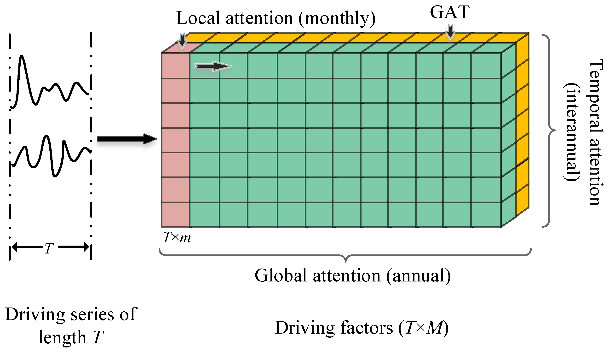
Previous researches have demonstrated that global climate indices significantly impact runoff across various time scales [50,51]. The uneven distribution of precipitation across various temporal and spatial dimensions influences runoff [52]. However, previous studies forecasted monthly runoff using global climate indices and precipitation data failed to adequately extract complex input factor information from the various dimensions, thereby compromising predictive accuracy. Li et al. [53] have demonstrated that local and global attention mechanisms possess advantages in identifying crucial local and global information in input images. Additionally, Fan et al. [54] have shown that temporal attention mechanisms can effectively extract important information from time series. Therefore, the study proposed the LGTA to individually extract information on monthly, annual, and interannual scales from global climate indices, and integrated GAT and LGTA to extract crucial topological information from precipitation and remotely-sensed elevation data. As shown in Figure 2, the timeseries driving data represent the timestep T of the deep learning model. The yellow blocks represented precipitation data of length T in the driving series, with a data structure of T × M. The GAT was utilized to extract temporal and spatial information from the time series of precipitation data at driving series T.

The green blocks in Figure 2 represented the time series of global climate indices at driving series T, with a data structure of T × M. The sliding window (highlighted in pink in Figure 2) was designed to compute the rolling local attention weight for each month within the historical monthly dataset of the global climate indices. The physical significance of the weight was its representation of the extent to which the global climate indices affect predicted monthly runoff on the monthly scale. The sliding window had a size of 1 month, with the sliding historical sequence spanning one year. The global climate indices matrix for each month was T × m, in which m represented the number of global climate indices for each month. The variations in global climate indices and value of m vary each month.

The present study applied the global attention mechanism to extract crucial information from all precipitation and global climate indices for the historical month (T × M). The physical significance of the global attention mechanism was its representation of the influence of input factors on predicted monthly runoff at the annual scale. Finally, the temporal attention mechanism was used to extract the weights of input factors at the forcing data series T, which represented the impacts of input factors on predicted monthly runoff at the interannual time scale.

2.1.3. The Structure of the GAT–LGTA–LSTM Model

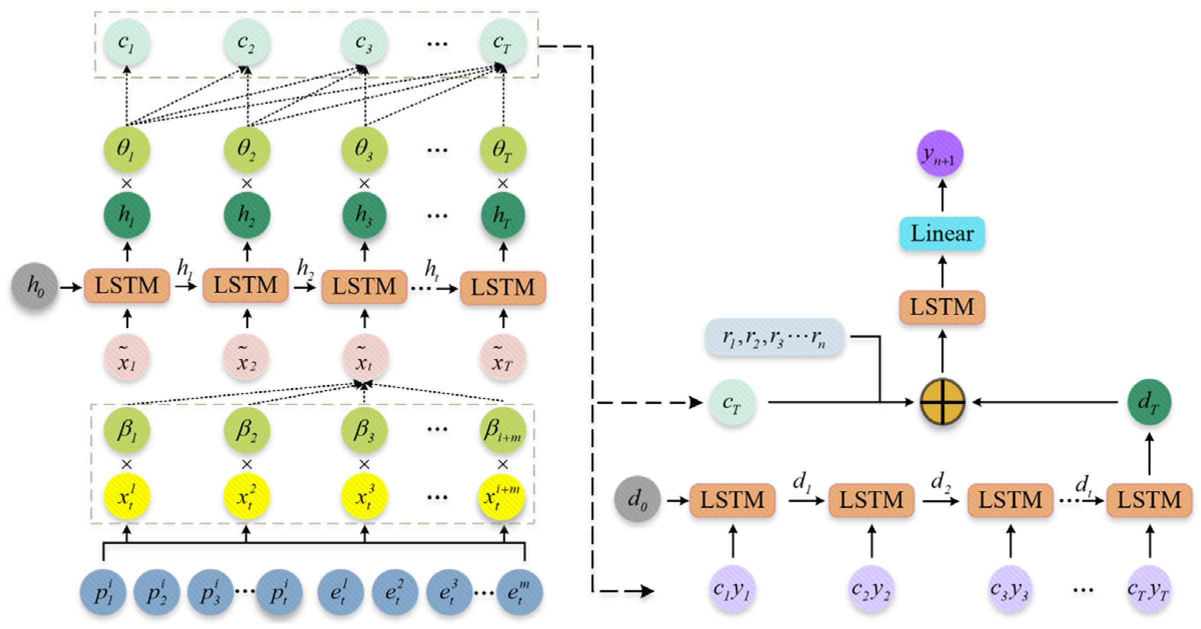
The LSTM model exhibits significant potential for development due to its excellent performance and physical interpretability in the field of streamflow forecasting [55,56,57]. Consequently, the GAT–LGTA–LSTM model was constructed by integrating GAT, LGTA, and LSTM. The inputs to the model include precipitation data and global climate indices. The model performed rolling predictions of monthly runoff. The present study used precipitation and global climate indices with strong correlations to the forecast month for simulate monthly runoff. Figure 3 shows the structure of GAT–LGTA–LSTM. The steps following in application of the model are outlined below.

(1) The GAT was used to process the input historical monthly precipitation data $\left\{P_1^i,P_2^i,\dots P_t^i,P_T^i\right\}$ based on remotely sensed elevation data, where i is number of meteorological stations and T is the length of the driving data series; $\left\{p_t^1,p_t^2,\dots p_t^i\right\}$ represented the historical monthly precipitation data at time t. The geographical topological precipitation series denoted as $\left\{g_t^1,g_t^2,\dots g_t^i\right\}$ at the time t was obtained by GAT, which includes topological information from different meteorological stations. Meanwhile, the global climate indices with a strong correlation $\left\{E_1^m,E_2^m,\dots E_t^m,E_T^m\right\}$ were also input to the model, where m denotes the numbers of global climate indices. The global climate indices at time t were denoted as $\left\{e_t^1,e_t^2,\dots e_t^m\right\}$ and were generated using the tanh function. Softmax was then employed for activating different local attention weights, as follows:

$${\alpha }_t^k=softmax(e_t^k)={\displaystyle \frac{\exp (v^t\tanh (\mathbf{W}{e}^k+b))}{{\displaystyle \sum _{k=1}^m\exp (v^t\tanh (\mathbf{W}{e}^m+b))}}}$$

(6)

where ${\alpha }_t^k$ denotes the weight of the k-th feature at the time t and $v^t$, $\mathbf{W}$, and $b$ are the parameters to be learned by the model.

The local attention weight was assigned to the input monthly global climate indices $\left\{e_t^1{\alpha }_t^1,e_t^2{\alpha }_t^2,\dots e_t^m{\alpha }_t^m\right\}$ at time t, respectively.

(2) The processed precipitation series at time t $\left\{g_t^1,g_t^2,\dots g_t^i\right\}$ was combined with the global climate indices series $\left\{e_t^1{\alpha }_t^1,e_t^2{\alpha }_t^2,\dots e_t^m{\alpha }_t^m\right\}$, thereby generating the new series $\left\{x_t^1,x_t^2,\dots x_t^{i+m}\right\}$. The global attention weight was calculated as

$${\beta }_t^k={\displaystyle \frac{\exp (v^T\tanh (\mathbf{W}[h_{t-1};s_{t-1}]+U{x}^k))}{{\displaystyle \sum _{k=1}^{i+m}\exp (v^T\tanh (\mathbf{W}[h_{t-1};s_{t-1}]+U{x}^{i+m})}}}$$

(7)

where ${\beta }_t^k$ is the weight of the k-th feature at time t; $v^T$, $\mathbf{W}$, and $U$ are the parameters to be learned in the model; and $h_{t-1}$ and $s_{t-1}$ denote the hidden state and cell state of the LSTM cell at time t − 1, respectively.

The global attention weight was assigned to the series at time t $\left\{x_t^1,x_t^2,\dots x_t^{i+m}\right\}$ as $x_t={\beta }_1{x}_1^{i+m},{\beta }_2{x}_2^{i+m},\dots {\beta }_t{x}_t^{i+m}$, and the result of all the time series $\left\{{\tilde{x}}_{\mathit{1}},{\tilde{x}}_2,\dots {\tilde{x}}_t\right\}$ were used as input to the LSTM cells.

(3) The series $\left\{{\tilde{x}}_1,{\tilde{x}}_2,\dots {\tilde{x}}_t\right\}$ was processed by the LSTM cells and the hidden state of every timestep $\left\{h_1,h_2,\dots h_T\right\}$ was extracted. Temporal attention was calculated as

$${\theta }_{t\prime }^t={\displaystyle \frac{\exp (v^T\tanh (\mathbf{W}[d_{t\prime -1};s_{t\prime -1}^{\prime }]+U{h}_t))}{{\displaystyle \sum _{t=1}^T\exp (v^T\tanh (\mathbf{W}[d_{t\prime -1};s_{t\prime -1}^{\prime }]+U{h}_T)}}}$$

(8)

where ${\theta }_{t\prime }^t$ is the weight of the timestep t at time $t\prime$; $v^T$, $\mathbf{W}$, and $U$ are the parameters to be learned during model training; and $d_{t\prime -1}$ and $s_{t\prime -1}^{\prime }$ denote the hidden state and cell state of the LSTM cell at time $t\prime -1$, respectively.

The temporal attention was assigned to the hidden state series of every timestep as $\left\{{\theta }_1{h}_1,{\theta }_2{h}_2,\dots {\theta }_T{h}_T\right\}$, and the context vector of every timestep was calculated as

$$c_{t\prime }={\displaystyle {\sum }_{t=1}^T{\theta }_{t\prime }^T}{h}_t$$

(9)

where $t\prime$ denotes the time required for calculating the context vector.

(4) Data on the monthly runoff series and context vector were combined as

$$y_{t\prime }={{\displaystyle w}}^t[y_{t\prime };c_{t\prime }]+\tilde{b}$$

(10)

where ${\tilde{y}}_{t\prime }$ is the combined result at time $t\prime$; $y_{t\prime }$ denotes the monthly runoff series at time 1 to $t\prime$; and ${{\displaystyle w}}^t$ and $\tilde{b}$ are the weight matrix and bias vectors, respectively.

The series $\left\{{\tilde{y}}_1,{\tilde{y}}_2,\dots {\tilde{y}}_T\right\}$ was input into the LSTM cells, with a d_T representing the final output of the LSTM cells.

(5) The c_T, d_T, and continuous historical runoff for the past H months of the prediction target month $\left\{r_1,r_2,r_3,\dots r_n\right\}$ were concatenated and input into the LSTM. The linear layer was used to obtain the final result $y_{n+1}$ from the output of LSTM.

2.1.4. Comparative Models

The present study compared five models to the proposed GAT–LGTA–LSTM model, namely LGTA–LSTM, GAT–GTA–LSTM, GAT–LSTM, GAT–GA–LSTM, and GA–LSTM. Figure 4 and Figure 5 show the architectural details of the GTA–LSTM and GA–LSTM models, respectively. The GTA–LSTM model was based upon the GAT–LGTA–LSTM model, although it excluded GAT and the local attention mechanism while retaining the global and temporal attention mechanisms. The GA–LSTM model was derived from the GTA–LSTM model, with the temporal attention mechanism excluded while the global attention mechanism was retained. The GA–LSTM model is essentially the attention-LSTM model, which was taken as the benchmark model [58]. The remaining LGTA–LSTM, GAT–LSTM, and GA–LSTM models were derived from the GAT–LGTA–LSTM, the GAT–GTA–LSTM, and GAT–GA–LSTM models, respectively, with the removal of GAT and are not discussed in more detail in section.

2.2. Maximal Information Coefficient

Reshef et al. [59] proposed the MIC for quantifying relationships between two continuously distributed random variables. The value of the MIC falls between 0 and 1 and represents the strength of a correlation. The present study applied this approach to identify correlations between global climate indices and runoff. The mutual information was given as

$$MIC(D,X,Y)=\underset{XY<B(\left|D\right|)}{\max }{\displaystyle \frac{I^{\ast }(D,X,Y)}{{\log }_2\min \left\{X,Y\right\}}}=\underset{XY<B(\left|D\right|)}{\max }{\displaystyle \frac{{\max }_{G}I(D|G)}{{\log }_2\min \left\{X,Y\right\}}}$$

(11)

where variable X = $\left\{x_i,i=1,2,\dots ,n\right\}$ and variable Y = $\left\{y_i,i=1,2,\dots ,n\right\}$; n is the length of variable; D = $\left\{(x_i,y_i),i=1,2,\dots ,n\right\}$ and is a set of ordered pairs; $\left|D\right|$ is the length of the dataset D; D|G represents the probability distribution formed by the data D across the cells of grid G; I(D|G) is the mutual information; and B is the upper bound of the grid size, which is often set to $n^{0.6}$.

Then, the Hampel test [60] was applied to select the global climate indices that are strongly correlated with the runoff for each month, based on the results of MIC.

2.3. Performance Metrics

The Nash–Sutcliffe coefficient of efficiency (NSE), Kling–Gupta Efficiency (KGE), mean absolute error (MAE), and mean absolute percentage error (MAPE) were used to evaluate the performances of the prediction models. These performance metrics are extensively utilized in the performance assessment of prediction models [61,62,63]. The NSE is utilized to quantify the forecasting accuracy of prediction models. The NSE value ranges from negative infinity to 1, with values closer to 1 indicating higher model prediction accuracy. The KGE combines three statistical metrics, the correlation coefficient, variability ratio, and bias ratio, into a single measure of model performance. The KGE ranges between -infinity and 1, where a value of 1 indicates perfect agreement between the model predictions and the observed data. The MAE reflects the average absolute error between the predicted and observed values. The MAPE represents the relative error between the predicted and observed values expressed as a percentage, placing greater emphasis on relative error. The MAE and MAPE have a range from 0 to positive infinity, with smaller values indicating higher model accuracy.

The coefficient of determination (R²) was used to evaluate the correlation between the observed and predicted monthly runoff. The performance metrics are expressed as follows:

$$\mathrm{NSE}=1-{\displaystyle \frac{{\displaystyle {\sum }_{i=1}^N{(y_i-{\widehat{y}}_i)}^2}}{{\displaystyle {\sum }_{i=1}^N{(y_i-\overline{y})}^2}}}$$

(12)

$$\mathrm{KGE}=1-\sqrt{{(\lambda -1)}^2+{(\gamma -1)}^2+{(R-1)}^2}$$

(13)

$$\mathrm{MAE}={\displaystyle \frac{{\displaystyle {\sum }_{i=1}^N\left|y_i-{\widehat{y}}_i\right|}}{N}}$$

(14)

$$\mathrm{MAPE}={\displaystyle \frac{1}{N}}{\displaystyle {\sum }_{i=1}^N\left|\frac{y_i-{\widehat{y}}_i}{y_i}\right|}$$

(15)

$${\mathrm{R}}^2={\left({\displaystyle \frac{{\displaystyle {\sum }_{i=1}^N(y_i-\overline{y})({\widehat{y}}_i-\overline{\widehat{y}})}}{\sqrt{{\displaystyle \sum _{i=1}^N{(y_i-\overline{y})}^2}}\sqrt{{\displaystyle \sum _{i=1}^N{({\widehat{y}}_i-\overline{\widehat{y}})}^2}}}}\right)}^2$$

(16)

where N is the count of observations; $y_i$ and ${\widehat{y}}_i$ represent the observed and predicted monthly runoff at time I, respectively; $\overline{y}$ and $\overline{\widehat{y}}$ represent the average value of observed and predicted monthly runoff, respectively; $\lambda ={\mu }_{\widehat{y}}/{\mu }_y$ is the mean bias and $\gamma ={\sigma }_{\widehat{y}}/{\sigma }_y$ is the variability bias; and $\mu$ and $\sigma$ are the mean and standard deviation, respectively.

3. Study Area and Model Parameters

3.1. Data and Study Area

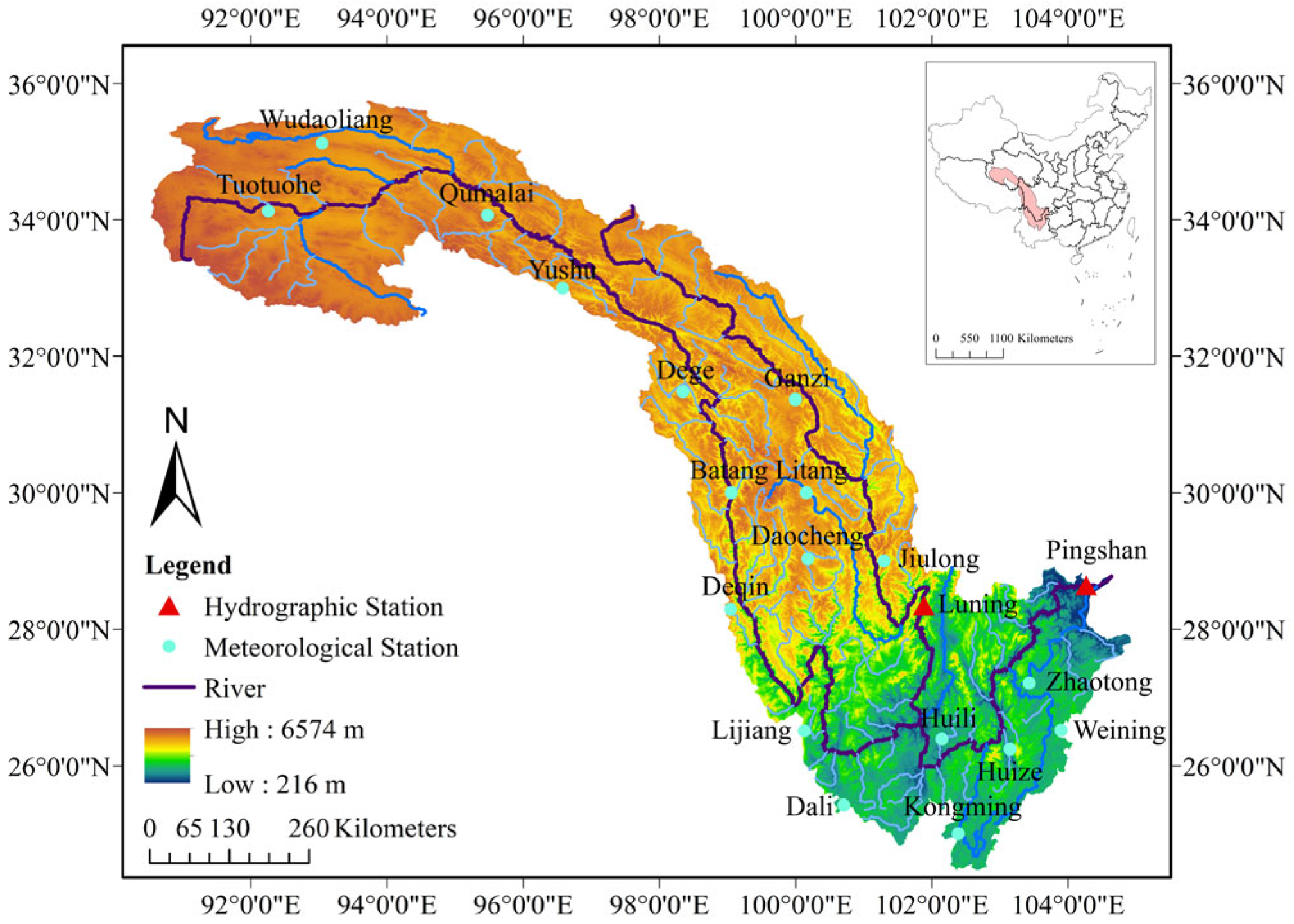
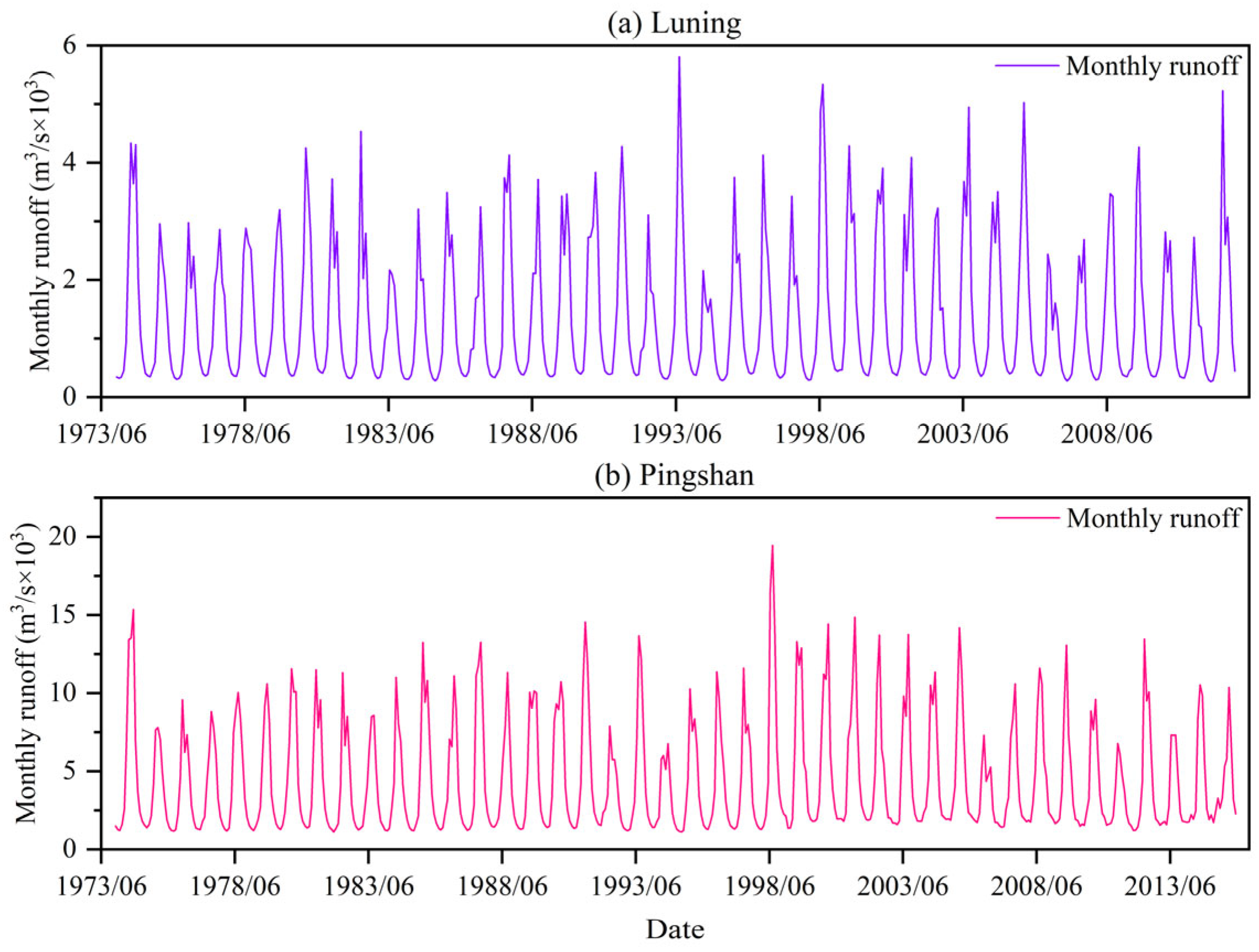
The Jinsha River forms part of the upper reaches of the Yangtze River basin. The basin covers a catchment area of 387,540 km², with a total length of 3481 km. The multi-year average rainfall ranges from 550 to 1650 mm, and the annual evapotranspiration ranges from 329.2 to 430.6 mm [64,65]. The average annual runoff of the Jinsha River is 145 billion m³ [66]. Figure 6 shows the spatial distribution of river systems, meteorological stations, and hydrological stations in the study area. Monthly observed runoff measured at the Luning and Pingshan hydrological station was provided by the Hydrological Bureau of the Yangtze River Water Resources Commission. The runoff series at the study site is shown in Figure 7. All runoff sequences have no missing values and exhibit strong seasonality. The runoff dataset covers the Luning station from January 1974 to December 2012, spanning 468 months. The dataset was divided into a training dataset (1974–2005) and test dataset (2006–2012). The runoff dataset was of Pingshan station from January 1974 to December 2015, spanning 504 months. The dataset was divided into a training dataset (1974–2006) and a test dataset (2007–2015). Monthly precipitation data were obtained from the Meteorological Data Center of the China Meteorological Administration. Meanwhile, global climate indices relevant to the study area were selected to forecast monthly runoff, as shown in

Table 1. Information of selected global climate indices.

Categories	Number	Name	Description
Climate indices	01	WPSH	Western Pacific Subtropical High Ridge Position Index
	02	APV	Asia Polar Vortex Intensity Index
	03	NHPV	Northern Hemisphere Polar Vortex Central Intensity Index
	04	EAT	East Asian Trough Intensity Index
	05	TPR1	Tibet Plateau Region 1 Index
	06	TPR2	Tibet Plateau Region-2 Index
	07	AO	Arctic Oscillation
	08	NAO	North Atlantic Oscillation
	09	PNA	Pacific North American Index
	10	AZC	Asian Zonal Circulation Index
Sea Surface Temperature (SST) Indices	11	Niño 1 + 2	Extreme Eastern Tropical Pacific SST (0–10S, 90–80W)
	12	Niño 3	Eastern Tropical Pacific SST (5N–5S, 150–90W)
	13	Niño 4	Central Tropical Pacific SST (5N–5S, 160E−150W)
	14	Niño 3.4	East Central Tropical Pacific SST (5N–5S, 170–120W)
	15	Niño A	Western Tropical Pacific SST (25N–35N, 130–150E)
	16	WHWP	Western Hemisphere Warm Pool Index
	17	IOWP	Indian Ocean Warm Pool Strength Index
	18	WPWP	Western Pacific Warm Pool Area Index
	19	AMO	Atlantic Multi-decadal Oscillation Index
Other Indices	20	SOI	Southern Oscillation Index
	21	QBO	Quasi-Biennial Oscillation Index

. These indices have been proven to exert either a direct or teleconnected influence on the study area [67,68,69,70]. The indices were obtained from the National Climate Center of the China Meteorological Administration. The detail the global climate indices selected by Hampel test for each month are given in Appendix A,

Table A1. Highly correlated global climate indices selected by the Hampel test.

Hydrographic Station	Prediction Month	Number	Name	Related Index Month
Pingshan	December	09	PNA	January
		20	SOI	January
		09	PNA	March
		19	AMO	June
		05	TPR1	August
		06	TPR2	August
		19	AMO	August
		06	TPR2	November
	January	18	WPWP	August
		19	AMO	August
		18	WPWP	September
	February	18	WPWP	March
		17	IOWP	June
		18	WPWP	June
		18	WPWP	July
		18	WPWP	August
		19	AMO	August
		18	WPWP	September
	March	16	WHWP	August
		18	WPWP	August
		19	AMO	August
		18	WPWP	September
		18	WPWP	October
	April	17	IOWP	January
		06	TPR2	March
		20	SOI	March
		18	WPWP	August
		19	AMO	August
		07	AO	October
		18	WPWP	October
	May	05	TPR1	April
		06	TPR2	April
		08	NAO	April
		19	AMO	May
		15	Niño A	October
		08	NAO	October
		02	APV	November
		06	TPR2	December
		21	QBO	December
	June	11	Niño 1 + 2	January
		12	Niño 3	February
		01	WPSH	May
	July	15	Niño A	January
		11	Niño 1 + 2	January
		19	AMO	February
		17	IOWP	June
		09	PNA	August
	August	19	AMO	February
		02	APV	April
		12	Niño 3	April
		09	PNA	August
		03	NHPV	September
		04	EAT	November
	September	19	AMO	March
		21	QBO	April
		02	APV	July
		03	NHPV	August
		08	NAO	August
	October	16	WHWP	April
		05	TPR1	September
		06	TPR2	September
		04	EAT	September
	November	20	SOI	January
		13	Niño 4	July
		06	TPR2	October
		04	EAT	October
Luning	December	06	TPR2	November
		15	Niño A	June
		19	AMO	June
	January	06	TPR2	December
		18	WPWP	August
		19	AMO	August
	February	06	TPR2	January
		18	WPWP	July
		07	AO	December
	March	16	WHWP	August
		15	Niño A	June
		18	WPWP	August
		06	TPR2	February
	April	18	WPWP	September
		06	TPR2	March
		18	WPWP	October
	May	21	QBO	July
		16	WHWP	September
		02	APV	October
		10	AZC	October
		06	TPR2	April
	June	01	WPSH	May
		11	Niño 1 + 2	January
		21	QBO	July
	July	19	AMO	February
		12	Niño 3	May
		21	QBO	June
		09	PNA	August
		15	Niño A	January
		11	Niño 1 + 2	January
	August	12	Niño 3	April
		09	PNA	August
		03	NHPV	September
		10	AZC	November
	September	07	AO	February
		03	NHPV	August
		02	APV	August
	October	10	AZC	March
		09	PNA	April
		13	Niño 4	September
		06	TPR2	September
	November	16	WHWP	March
		19	AMO	June
		06	TPR2	October
		08	NAO	August

. The lengths of the precipitation and global climate indices time series aligned with the runoff time series.

3.2. Hyperparameters of Models and Settings

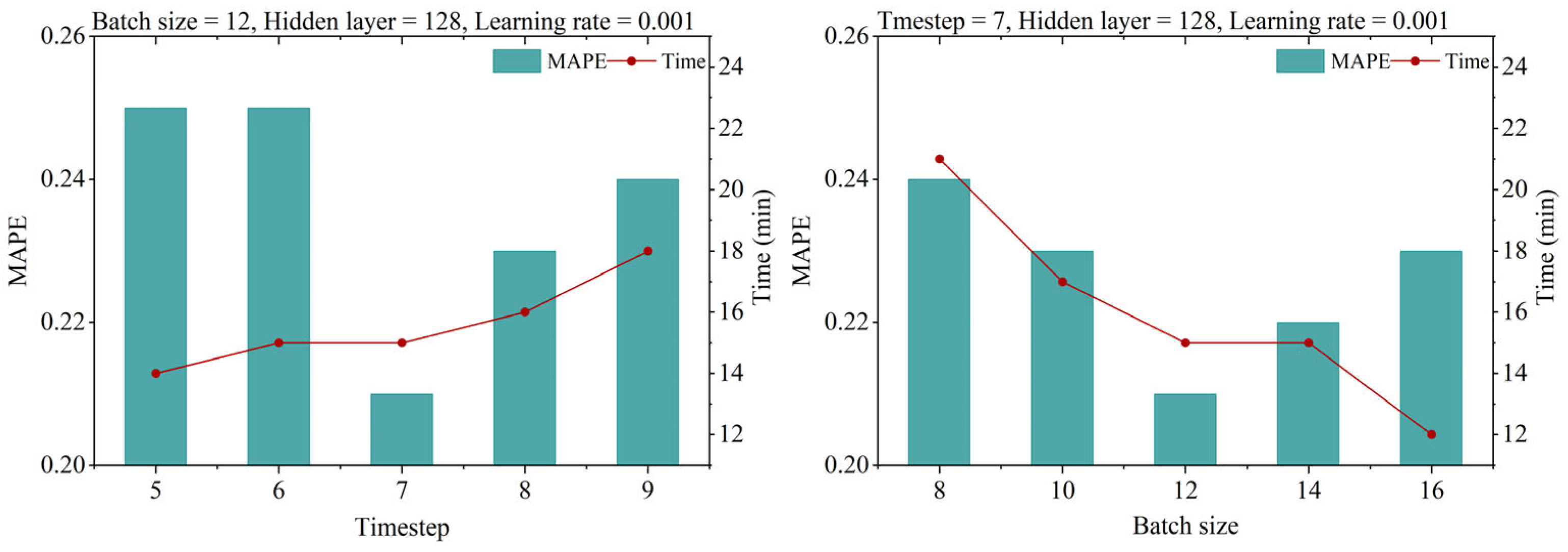
In this study, the Grey Wolf Optimizer (GWO) algorithm selected the optimal combination of model hyperparameters [71]. For the proposed model, batch size and timestep are the key hyperparameters influencing model performance. The average MAPE and average training time of the GAT–LGTA–LSTM model were analyzed based on variations in these hyperparameters (Figure 8). As shown in Figure 8, when other hyperparameters remain unchanged, both an increase or decrease in the time step and batch size leads to an increase in MAPE. Meanwhile, as the time step and batch size increase, the training time of the proposed model gradually increases, with the batch size showing the most significant impact. Therefore, the present study employed a batch size and time step of 12 and 7, respectively. All models utilized a hidden layer with 128 neurons. The initial learning rate was set to 0.001. The maximum train epoch was defined as 300. The Pytorch 1.8 framework in Python 3.8 was utilized to develop the models. The computer hardware specifications used in the present study are NVDIA GeForce GTX 1650 Ti with Max-Q Design and Intel(R) Core (TM) i7-10750H CPU with 32 GB Memory. The computation time for the six models ranged from 30 to 40 min. All the prediction models were repeated ten times, followed by the computation of average values for each evaluation index.

4. Results

4.1. Model Comparison and Analysis

Table 2. The monthly runoff forecasting performances of the graph attention network (GAT)–local–global–temporal attention mechanism, (LGTA)–long–short term memory (LSTM) model, and other comparative prediction models.

Station	Model	Training				Testing
		NSE	KGE	MAPE	MAE (m3/s)	NSE	KGE	MAPE	MAE (m3/s)
Luning	GAT–LGTA–LSTM	0.90	0.92	0.22	225.83	0.87	0.88	0.24	251.59
	LGTA–LSTM	0.88	0.91	0.23	241.64	0.85	0.86	0.26	287.42
	GAT–GTA–LSTM	0.87	0.89	0.24	257.28	0.82	0.82	0.29	303.18
	GTA–LSTM	0.85	0.86	0.26	275.72	0.80	0.80	0.35	344.75
	GAT–GA–LSTM	0.86	0.86	0.25	263.85	0.81	0.81	0.32	312.74
	GA–LSTM	0.85	0.88	0.26	281.11	0.80	0.80	0.35	330.65
Pingshan	GAT–LGTA–LSTM	0.92	0.92	0.16	642.19	0.89	0.91	0.18	683.29
	LGTA–LSTM	0.90	0.91	0.23	720.01	0.86	0.87	0.25	812.33
	GAT–GTA–LSTM	0.89	0.89	0.24	739.55	0.83	0.84	0.27	869.98
	GTA–LSTM	0.89	0.89	0.25	750.50	0.81	0.81	0.30	995.08
	GAT–GA–LSTM	0.88	0.89	0.25	784.06	0.82	0.83	0.27	893.82
	GA–LSTM	0.88	0.88	0.25	769.46	0.81	0.82	0.31	920.79

provides a summary of the performances of the GAT–LGTA–LSTM model and five other comparative models. For the two stations, the GAT–LGTA–LSTM model outperformed the other models in most cases, exhibiting higher average NSE and KGE. The GAT–LGTA–LSTM also produced lower average MAPE and MAE. The LGTA–LSTM model showed the second-best performance. The smaller difference in average NSE and KGE between the training and test periods for the GAT–LGTA–LSTM model compared to those of the other models was further confirmation of the robustness of the GAT–LGTA–LSTM model. During the testing period, the GAT–LGTA–LSTM model achieved NSE values of 0.87 and 0.89 at Luning and Pingshan stations, respectively. For the predictions on the Pingshan and Luning test datasets, the GAT–LGTA–LSTM model improved NSE by 0.07 and 0.08 and KGE by 0.08 and 0.09, reduced MAPE by 0.11 and 0.13, and decreased MAE by 78.41 m³/s and 237.5 m³/s, respectively, compared to the GA–LSTM benchmark model. Meanwhile, the NSE and KGE values of LGTA–LSTM exceeded those of GTA–LSTM by 0.05 and 0.06 at Luning and Pingshan stations, respectively. Furthermore, both MAPE and MAE of the LGTA–LSTM were lower than those of the GTA–LSTM at both stations. The results suggested that the local attention mechanism based on global and temporal attention mechanisms can enhance the ability of the model to extract information from global climate indices.

The performances of GAT–LGTA–LSTM, GAT–GTA–LSTM, and GAT–GA–LSTM models over the test period exceeded those of the LGTA–LSTM, GTA–LSTM, and GA–LSTM models at both the Luning and Pingshan stations. The result further confirmed that GAT improves the ability of a model to forecast monthly runoff by extracting spatial topological structures and remote sensing elevation information of meteorological stations. At the two stations, the incorporation of the GAT resulted in the most significant accuracy improvement in the LGTA–LSTM model compared to the GTA–LSTM and GA–LSTM models. Following the incorporation of the GAT into the LGTA–LSTM model at Luning Station, the NSE increased by 0.02, KGE increased by 0.02, MAPE decreased by 0.02, and MAE dropped by 35.83 m³/s. Similarly, at Pingshan Station, the addition of GAT resulted in a 0.03 increase in NSE, a 0.04 improvement in KGE, a 0.07 reduction in MAPE, and a 129.04 m³/s decrease in MAE. This suggests that the combination of GAT and LGTA results in the most substantial enhancement in both model accuracy and robustness.

4.2. Evaluation of Prediction Results

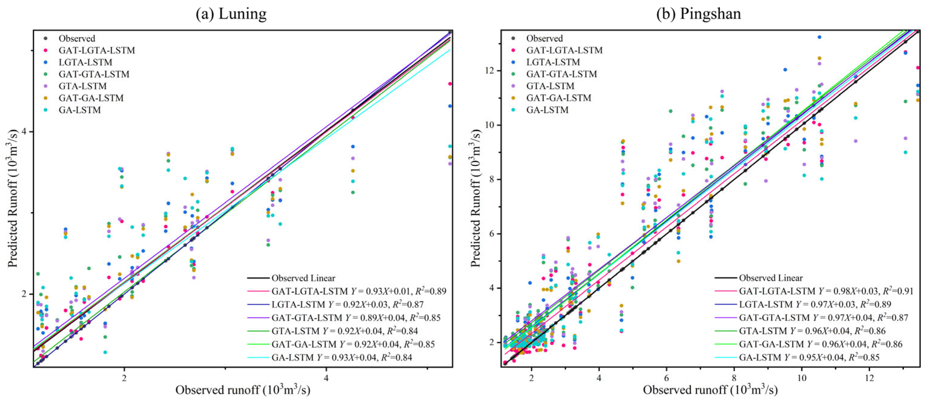
Figure 9 summarizes the predictive capabilities of the assessed models. For the two stations, the compared models generally overestimated and underestimated low and high runoff when compared to observed values, respectively. In contrast, the predictions of runoff by the GAT–LGTA–LSTM model were, in general, more reflective of observed runoff, particularly the low and high extremes, obtaining the highest R² at the Luning and Pingshan station. The incorporation of GAT based on GA, GTA, and LGTA increased model performance by an R² range of 0.1 to 0.2. For two stations, the incorporation of a local attention mechanism in the models has resulted in R² increases of 0.2 and 0.3, consistent with the findings in Table 2.

Figure 10 displays the predicted and observed values at the Luning and Pingshan stations during the test period. As shown in Figure 10, at the two stations, all assessed models performed well in predicting high runoff. However, some models overestimated higher runoff. At the Luning station, the high monthly runoff predictions of the GAT–LGTA–LSTM model for the years 2006, 2009, and 2012 are closer to the observed values. All comparative models generally overestimated lower runoff, while the GAT–LGTA–LSTM model yielded a more accurate representation of lower runoff, particularly for the years 2008 and 2009. At the Pingshan station, the GAT–LGTA–LSTM model provided estimates of high runoff that were closer to observed values, including in 2007, 2010, 2011, and 2014. In forecasting low monthly runoff, the GAT–LGTA–LSTM model also demonstrated superior predictive performance for the years 2007, 2010, and 2012, relative to other models. As shown in Figure 9 and Figure 10, at the two stations, all of the assessed models performed well in forecasting high monthly runoff in the test period, whereas the GAT–LGTA–LSTM model achieved the best performance, particularly in low runoff predictions.

4.3. Visual Attention Analysis

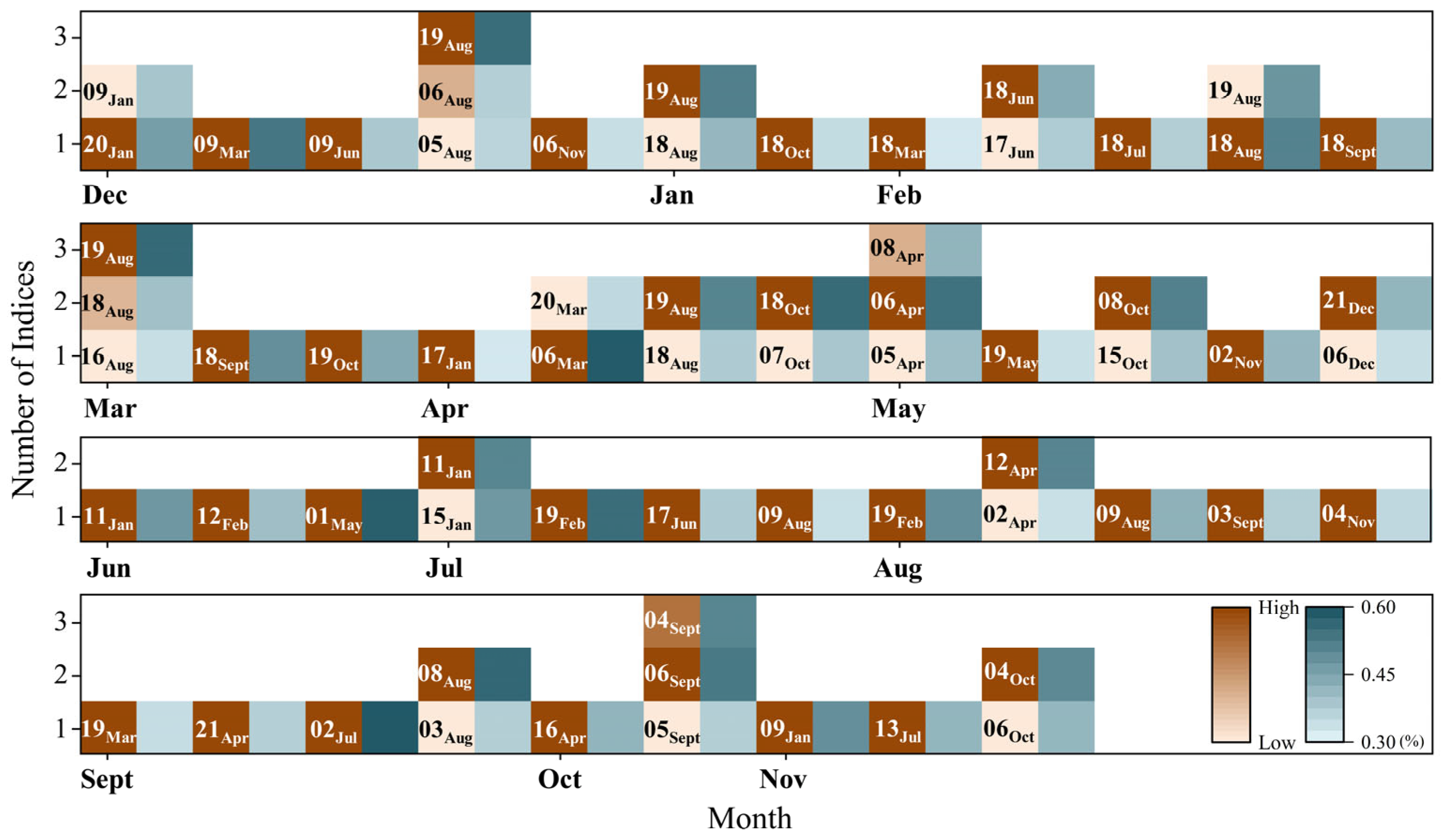
The present study explored the weights of local, global, and temporal attention mechanisms in the GAT–LGTA–LSTM model by visualizing local attention on global climate indices and global attention weights for both precipitation and global climate indices. Taking the Pingshan station as an example, the average local, global, and temporal attention weights in the GAT–LGTA–LSTM model were calculated by running 10 times. A more intuitive representation of the weight allocation of global climate indices was achieved by grouping the local attention weights of global climate indices with their corresponding global attention weights in Figure 11. There were differences in the average weights of indices among the different months due to the varying number of factors in each month. Therefore, the terms “high” and “low” were used to describe the magnitude of local attention weights for each month. As shown in Figure 11, indices with a high local attention weight did not necessarily have a high global attention weight. However, indices with a high global attention weight tended to have a correspondingly high local attention weight. When the local and global attention weights of the index are both high, it indicates a significant contribution to runoff forecasting.

Furthermore, different global climate indices exhibited distinct local and global weights in different seasons and months. The AMO and WPWP demonstrated a greater weight for winter and spring runoff forecasting. And the TPR2 played a significant role in the spring runoff forecasting. The WPSH, Niño 1 + 2, and Niño 3 provided substantial contributions to summer runoff forecasting. Meanwhile, the EAT, APV, and NAO exhibited higher local and global attention weights in autumn runoff forecasting, which indicates significant contributions. However, the contributions of indices such as IOWP, AO, PNA, and SOI to monthly runoff prediction are not significant across various months. The results indicated that, within the same monthly scale, the contributions of global climate indices to monthly runoff predictions vary significantly. Furthermore, various global climate indices contribute differently to runoff predictions across distinct months.

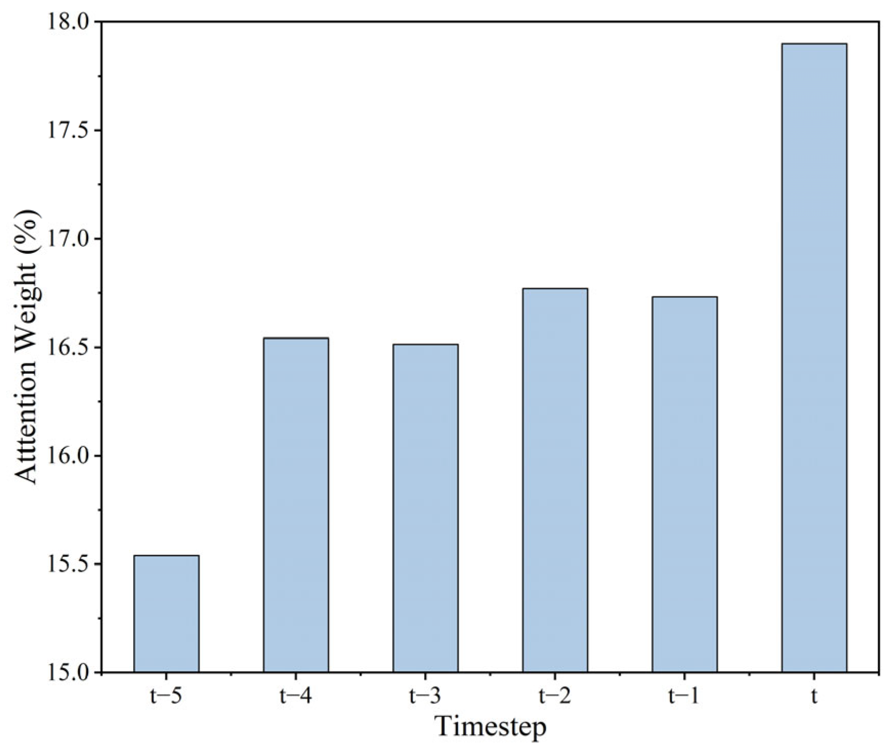
The global attention distribution of precipitation is shown in Figure 12. It can be observed that meteorological stations located closer to the hydrological stations were assigned a higher proportion of the global attention weight for the month preceding the prediction month. The global attention weight gradually decreased with increasing distance between meteorological stations and the hydrological station. In addition, the global attention weight for precipitation decreased over time. The results indicated that the global attention integrated with GAT effectively extracts crucial precipitation information across both temporal and spatial dimensions. The interannual weight of all input factors is illustrated in Figure 13. It can be found that factors from the year preceding the prediction month were assigned higher weights in the GAT–LGTA–LSTM model, with these weights decreasing over time.

5. Discussion

The results indicated the GAT–LGTA–LSTM model achieved the best accuracy in predicting runoff among the assessed models at Luning and Pingshan stations. Xiong et al. [21] used 50 years of continuous runoff data to predict monthly runoff at Pingshan Hydrological Station, achieving a maximum coefficient of determination of 0.86. Han et al. [39] found that the traditional physical model, the two-parameter monthly water balance (TWB) model, using precipitation and potential evapotranspiration over a 49-year time series as inputs as inputs, achieved a prediction NSE of 0.83 at Pingshan Station. The GAT–LGTA–LSTM model, assessed in the present study, was trained on 42 years of data and achieved an NSE of 0.89 at Pingshan station. Therefore, the GAT–LGTA–LSTM applied to the Pingshan Hydrological Station improved forecasting accuracy using a shorter period of data. This result can be attributed to the more comprehensive input data included in the model, including remotely sensed elevation data, historical runoff, precipitation data, and global climate indices, as well as the distinct processing methods used for different types of input factors. The local attention mechanism and GAT were initially used to extract information for global climate indices and geographical topological characteristics of precipitation, respectively. Subsequently, this information was obtained using the global and temporal attention mechanisms. LSTM was used to extract information for the continuous historical runoff data.

5.1. Underlying Mechanisms Used in the Proposed Model for Extracting Global Climate Indices Information

The results of the present study showed that the addition of the local attention mechanism improved model prediction accuracy, resulting in average NSE increases of 0.04 and 0.05 at Luning and Pingshan stations, respectively. Mirsamadi et al. [64] demonstrated that the local attention mechanism can be used for focusing on specific regions of a speech signal that are more salient. The results indicated that the local attention mechanism enabled the extraction of monthly-scale global climate indices information, thereby significantly increasing the capacity of the model to capture global climate indices information. In addition, the local–global attention mechanisms enabled the efficient use of local and global information, thereby focusing on the most appropriate area of contextual frames [72,73,74]. As shown in the Section 4.3, synergistic integration of the local–global attention mechanisms enhanced both local and global weights, thereby capturing crucial global climate indices information.

The study area is located in the upper reaches of the Yangtze River Basin. Previous studies have demonstrated that indices such as the AMO, NAO, WPWP, Niño 1 + 2, Niño A, Niño 3.4, AO, and WPSH significantly influence summer precipitation in the Yangtze River Basin, consequently impacting runoff variability in the region [69,75,76,77,78,79,80,81]. Meanwhile, global climate indices such as AMO, EAT, and NHPVI can further affect the runoff in the Yangtze River Basin by influencing winter temperatures in the region [82,83,84,85]. This study indicates that these indices have varying attention weights and contributions to runoff prediction in the study area. In addition, the calculation of the elasticity coefficient for the global climate index (defined as the ratio of a ±10% fluctuation in the index to the corresponding change in predicted runoff) revealed that this index exhibits high sensitivity to runoff predictions (Figure 14). Specifically, the WPWP, TPR2, AMO, NAO, and WPSH demonstrate high sensitivity in model predictions, underscoring their significant impact on model outputs. Conversely, the IOWP, AO, and SOI exhibit lower sensitivity compared to other indices, aligning with the patterns outlined in Section 4.3.

However, while these global climate indices are associated with the meteorology of the study area, their contributions to monthly runoff prediction vary. Hence, it is essential to carefully consider the capabilities of global climatic indices in predicting monthly runoff within the same month scale. In addition, previous researches indicate that various global climate variables have distinct effects on monthly and seasonal climate [86,87,88]. The present study found that the global climate indices contribute differently to runoff forecasting in various months. Therefore, for forecasting monthly runoff, using a fixed set of indices for all months is unsuitable. Instead, it is recommended to select the indices corresponding to a specific season or month.

The present study determined the optimal timestep of the GAT–LGTA–LSTM model to be seven. This result indicated that optimal simulation of monthly runoff can be achieved using input data for the previous 6 years. The temporal attention mechanism assigned distinct weights to different historical years of the prediction month, with the weight increasing with decreasing distance to the historical year. This result can be attributed to the current year’s precipitation having the greatest impact on runoff in the forecast month [89,90]. Furthermore, the weights applied to the other years exhibit only slight decreases compared to that of the first historical year. For instance, the weight of the second historical year was only 1.1% lower than that of the first historical year, whereas that of the sixth year was 2.4% lower than that of the first historical year. The pattern could be attributed to the close relationship between most global climate indices and runoff during the previous historical years. Previous studies have demonstrated that El Niño, NAO, AMO, and WHWP significantly impact meteorological and hydrological factors in the Yangtze River Basin across different interannual scales [91,92,93,94,95].

5.2. Underlying Mechanisms Used in the Proposed Model to Extract Precipitation Information

Previous studies indicated that the GAT robustly extracts geographical topological information on meteorological stations based on remotely sensed elevation data [96]. In this study, the GAT provided the spatial topological information of the meteorological stations to the global attention mechanism. As shown in Section 4.3, the global attention mechanism effectively captured precipitation information across both temporal and spatial dimensions. Therefore, the performances of the prediction models were improved by the inclusion of GAT. In addition, the impact of a meteorological station on runoff increased with decreasing distance between the meteorological station and the Pingshan hydrological station, consistent with the findings of Chang et al. [97]. The results of the present study showed that precipitation concentrated in the first historical month had a significant impact on monthly runoff. Kai et al. [98] identified a lag of 20–30 d between precipitation and runoff in the Jinsha River basin, consistent with the results of the present study.

Furthermore, the greatest improvement in the GTA–LSTM model prediction was achieved when it was integrated with GAT and local attention mechanisms to produce the GAT–LGTA–LSTM model. At the Pingshan and Luning stations, the GAT–LGTA–LSTM model achieved NSE improvements of 0.07 and 0.08 and reductions in MAE of 93.16 m³/s and 311.79 m³/s, respectively, compared to the GTA–LSTM model. This improvement in prediction accuracy could be attributed mainly to (1) the ability of GAT to effectively extract geographical topological precipitation information to the global attention mechanism based on remotely sensed elevation information of meteorological stations [45] and (2) the ability of the local attention mechanism to highlight crucial global climate indices information while attenuating less important details [40]. This approach provided more meaningful local and global climate information for the global and temporal attention mechanisms than the equally weighting factor input method. Hence, the proposed model could significantly improve the prediction accuracy.

6. Conclusions

The present study proposed a novel monthly runoff prediction model (GAT–LGTA–LSTM) constructed by integrating GAT, LGTA, and LSTM. The data input into the proposed model include remotely sensed elevation data, global climate indices, precipitation, and runoff factors. The Jinsha River was selected as a case study. The performance of the GAT–LGTA–LSTM model was compared to those of five other models. The local, global, and temporal attention weights of inputs were analyzed to identify the underlying mechanisms of the proposed model. The main conclusions of the present study can be summarized as follows:

(1) The GAT–LGTA–LSTM model achieved the optimal performance in simulating runoff when compared to the other assessed models, particularly within the representation of low flows. The results indicated that the optimal estimation of runoff required the inclusion of local, global, and temporal attention mechanisms. The incorporation of the local attention mechanism along with GAT improved the accuracy and robustness of monthly runoff prediction.

(2) The results indicated that the GAT–LGTA–LSTM model can effectively capture the information provided by remote sensing elevation data. The optimal performance of the GAT–LGTA–LSTM model could be attributed to its capacity to effectively capture pivotal information associated with geographical topological precipitation data and global climate indices. The local attention mechanism assigns a higher weight to the key information of global climate indices at monthly time scales. Therefore, the incorporation of both local and global attention mechanisms in the model facilitated the detailed capture of global climate indices’ key information at monthly and annual time scales. In particular, the global attention mechanism combination with GAT allowed the more effective extraction of temporal and spatial precipitation data. Finally, the inclusion of the temporal attention mechanism allowed the extraction of important information for input factors at an interannual time scale, thereby improving the performance of the prediction model.

(3) For monthly runoff forecasting using global climate indices, it is necessary to select the appropriate set of predictive global climate indices more precisely for different seasons or months, rather than using a fixed set of indices to forecast runoff for all months.

(4) The proposed model is well-suited for long-term runoff forecasting tasks in water resource management, offering the advantage of acquiring topological precipitation information from remote sensing data and effectively integrating global climate indices. However, the application of the proposed model relies on the timely acquisition of various datasets, particularly global climate indies.

References

1. Sun, Z.; Liu, Y.; Zhang, J.; Hua, C.; Shu, Z. A Review of Medium-Long Term Runoff Prediction. Water Resour. Prot. 2023, 39, 10. [Google Scholar]
2. Yi, B.; Chen, L.; Yang, B.; Li, S.; Leng, Z. Influences of the Runoff Partition Method on the Flexible Hybrid Runoff Generation Model for Flood Prediction. Water 2023, 15, 2738. [Google Scholar] [CrossRef]
3. Zhou, F.; Chen, Y.; Liu, J. Application of a New Hybrid Deep Learning Model That Considers Temporal and Feature Dependencies in Rainfall–Runoff Simulation. Remote Sens. 2023, 15, 1395. [Google Scholar] [CrossRef]
4. Deb, P.; Kiem, A.S.; Willgoose, G. A linked surface water-groundwater modelling approach to more realistically simulate rainfall-runoff non-stationarity in semi-arid regions. J. Hydrol. 2019, 575, 273–291. [Google Scholar] [CrossRef]
5. Xie, K.; Liu, P.; Zhang, J.; Han, D.; Wang, G.; Shen, C. Physics-guided deep learning for rainfall-runoff modeling by considering extreme events and monotonic relationships. J. Hydrol. 2021, 603, 127043. [Google Scholar] [CrossRef]
6. Mehran, A.; AghaKouchak, A.; Phillips, T.J. Evaluation of CMIP5 continental precipitation simulations relative to satellite-based gauge-adjusted observations. J. Geophys. Res. Atmos. 2014, 119, 1695–1707. [Google Scholar] [CrossRef]
7. Xiang, Z.; Demir, I. Distributed long-term hourly streamflow predictions using deep learning–A case study for State of Iowa. Environ. Modell. Softw. 2020, 131, 104761. [Google Scholar] [CrossRef]
8. He, X.; Luo, J.; Li, P.; Zuo, G.; Xie, J. A hybrid model based on variational mode decomposition and gradient boosting regression tree for monthly runoff forecasting. Water Resour. Manag. 2020, 34, 865–884. [Google Scholar] [CrossRef]
9. Humphrey, G.B.; Gibbs, M.S.; Dandy, G.C.; Maier, H.R. A hybrid approach to monthly streamflow forecasting: Integrating hydrological model outputs into a Bayesian artificial neural network. J. Hydrol. 2016, 540, 623–640. [Google Scholar] [CrossRef]
10. Huang, S.; Chang, J.; Huang, Q.; Chen, Y. Monthly streamflow prediction using modified EMD-based support vector machine. J. Hydrol. 2014, 511, 764–775. [Google Scholar] [CrossRef]
11. Ashrafi, M.; Chua, L.H.C.; Quek, C.; Qin, X. A fully-online Neuro-Fuzzy model for flow forecasting in basins with limited data. J. Hydrol. 2017, 545, 424–435. [Google Scholar] [CrossRef]
12. An, T.; Feng, K.; Cheng, P.; Li, R.; Zhao, Z.; Xu, X.; Zhu, L. Adaptive prediction for effluent quality of wastewater treatment plant: Improvement with a dual-stage attention-based LSTM network. J. Environ. Manag. 2024, 359, 120887. [Google Scholar] [CrossRef] [PubMed]
13. Yuan, X.; Chen, C.; Lei, X.; Yuan, Y.; Muhammad Adnan, R. Monthly runoff forecasting based on LSTM–ALO model. Stoch. Environ. Res. Risk A 2018, 32, 2199–2212. [Google Scholar] [CrossRef]
14. Widya, L.K.; Rezaie, F.; Lee, W.; Lee, C.-W.; Nurwatik, N.; Lee, S. Flood susceptibility mapping of Cheongju, South Korea based on the integration of environmental factors using various machine learning approaches. J. Environ. Manag. 2024, 364, 121291. [Google Scholar] [CrossRef]
15. Kao, I.F.; Zhou, Y.; Chang, L.-C.; Chang, F.-J. Exploring a Long Short-Term Memory based Encoder-Decoder framework for multi-step-ahead flood forecasting. J. Hydrol. 2020, 583, 124631. [Google Scholar] [CrossRef]
16. Mo, R.; Xu, B.; Zhong, P.-A.; Dong, Y.; Wang, H.; Yue, H.; Zhu, J.; Wang, H.; Wang, G.; Zhang, J. Long-term probabilistic streamflow forecast model with “inputs–structure–parameters” hierarchical optimization framework. J. Hydrol. 2023, 622, 129736. [Google Scholar] [CrossRef]
17. Tursun, A.; Xie, X.; Wang, Y.; Liu, Y.; Peng, D.; Zheng, B. Enhancing streamflow simulation in large and human-regulated basins: Long short-term memory with multiscale attributes. J. Hydrol. 2024, 630, 130771. [Google Scholar] [CrossRef]
18. Marjani, M.; Mahdianpari, M.; Mohammadimanesh, F. CNN-BiLSTM: A Novel Deep Learning Model for Near-Real-Time Daily Wildfire Spread Prediction. Remote Sens. 2024, 16, 1467. [Google Scholar] [CrossRef]
19. Fang, W.; Qin, H.; Liu, G.; Yang, X.; Xu, Z.; Jia, B.; Zhang, Q. A Method for Spatiotemporally Merging Multi-Source Precipitation Based on Deep Learning. Remote Sens. 2023, 15, 4160. [Google Scholar] [CrossRef]
20. Song, P. Raw Water Supply System Operation and Risk Research with Considering Forecast Uncertainty under Low Water Scenario. Ph.D. Thesis, Zhejiang University, Zhejiang, China, 2021. [Google Scholar]
21. Xiong, Y.; Zhou, J.; Jia, B.; Hu, G. Monthly runoff prediction based on teleconnection factors selection using random forest model. J. Hydrol. Eng. 2022, 41, 32–45. [Google Scholar]
22. Urbanowicz, R.J.; Meeker, M.; La Cava, W.; Olson, R.S.; Moore, J.H. Relief-based feature selection: Introduction and review. J. Biomed. Inform. 2018, 85, 189–203. [Google Scholar] [CrossRef] [PubMed]
23. Li, M.-H.; Vu, T.M.; Chen, P.-Y. Multiple drought indices and their teleconnections with ENSO in various spatiotemporal scales over the Mekong River Basin. Sci. Total Environ. 2023, 854, 158589. [Google Scholar]
24. Qin, Y. Nonlinear Responses of Extreme Streamflow to Climate Variability in Europe. Ph.D. Thesis, East China Normal University, Shanghai, China, 2022. [Google Scholar]
25. Yao, L.; Libera, D.A.; Kheimi, M.; Sankarasubramanian, A.; Wang, D. The roles of climate forcing and its variability on streamflow at daily, monthly, annual, and long-term scales. Water Resour. Res. 2020, 56, e2020WR027111. [Google Scholar] [CrossRef]
26. Ogunjo, S.T.; Fuwape, I.A. Nonlinear characterization and interaction in teleconnection patterns. Adv. Space Res. 2020, 65, 2723–2732. [Google Scholar] [CrossRef]
27. Jiang, Z.; Xu, H.; Ma, J. Atmospheric Circulation Characteristics of Heavy Precipitation Events and Impact of Sea Surface Temperature over the Southern China in the Autumn of 2016. Chin. J. Atmos. Sci 2021, 45, 1023–1038. [Google Scholar]
28. Dong, L.; Zhang, P.; Liu, J.; Tong, X.; Xie, H. Combined influence of solar activity and ENSO on hydrological processes in Yoshino River basin, Japan. AWS Adv. Water Sci. 2017, 28, 671–680. [Google Scholar]
29. Zhang, M.; Su, H.; Wen, J. Classification of flower image based on attention mechanism and multi-loss attention network. Comput. Commun. 2021, 179, 307–317. [Google Scholar] [CrossRef]
30. Liu, Y.; Ge, K.; Zhang, X.; Lin, L. Real-time attention based look-alike model for recommender system. In Proceedings of the 25th ACM SIGKDD International Conference on Knowledge Discovery & Data Mining, Anchorage, AK, USA, 4–8 August 2019; pp. 2765–2773. [Google Scholar]
31. Zhao, D.; Shao, F.; Liu, Q.; Zhang, H.; Zhang, Z.; Yang, L. Improved Architecture and Training Strategies of YOLOv7 for Remote Sensing Image Object Detection. Remote Sens. 2024, 16, 3321. [Google Scholar] [CrossRef]
32. He, W.; Wu, Y.; Li, X. Attention mechanism for neural machine translation: A survey. In Proceedings of the 2021 IEEE 5th Information Technology, Networking, Electronic and Automation Control Conference (ITNEC), Xi’an China, 15–17 October 2021; pp. 1485–1489. [Google Scholar]
33. Zhang, F.; Kang, Y.; Cheng, X.; Chen, P.; Song, S. A hybrid model integrating Elman neural network with variational mode decomposition and Box–Cox transformation for monthly runoff time series prediction. Water Resour. Manag. 2022, 36, 3673–3697. [Google Scholar] [CrossRef]
34. Lim, B.; Zohren, S. Time-series forecasting with deep learning: A survey. Philos. Trans. R. Soc. A 2021, 379, 20200209. [Google Scholar] [CrossRef]
35. Gao, Y.; Ruan, Y. Interpretable deep learning model for building energy consumption prediction based on attention mechanism. Energy Build. 2021, 252, 111379. [Google Scholar] [CrossRef]
36. Zhang, L.; Qin, H.; Mao, J.; Cao, X.; Fu, G. High temporal resolution urban flood prediction using attention-based LSTM models. J. Hydrol. 2023, 620, 129499. [Google Scholar] [CrossRef]
37. Cui, Z.; Guo, S.; Zhou, Y.; Wang, J. Exploration of dual-attention mechanism-based deep learning for multi-step-ahead flood probabilistic forecasting. J. Hydrol. 2023, 622, 129688. [Google Scholar] [CrossRef]
38. Zhou, R.; Zhang, Y.; Wang, Q.; Jin, A.; Shi, W. A hybrid self-adaptive DWT-WaveNet-LSTM deep learning architecture for karst spring forecasting. J. Hydrol. 2024, 634, 131128. [Google Scholar] [CrossRef]
39. Han, D.; Liu, P.; Xie, K.; Li, H.; Xia, Q.; Cheng, Q.; Wang, Y.; Yang, Z.; Zhang, Y.; Xia, J. An attention-based LSTM model for long-term runoff forecasting and factor recognition. Environ. Res. Lett. 2023, 18, 024004. [Google Scholar] [CrossRef]
40. Huang, S.; Wang, D.; Wu, X.; Tang, A. Dsanet: Dual self-attention network for multivariate time series forecasting. In Proceedings of the 28th ACM International Conference on Information and Knowledge Management, Beijing, China, 3–7 November 2019; pp. 2129–2132. [Google Scholar]
41. Xiong, T.; He, J.; Wang, H.; Tang, X.; Shi, Z.; Zeng, Q. Contextual Sa-Attention Convolutional LSTM for Precipitation Nowcasting: A Spatiotemporal Sequence Forecasting View. IEEE J. Sel. Top. Appl. Earth Obs. Remote Sens. 2021, 14, 12479–12491. [Google Scholar] [CrossRef]
42. Liu, Z.; Wu, Y.; Ding, Y.; Feng, J.; Lu, T. Context and temporal aware attention model for flood prediction. In Proceedings of the Advances in Multimedia Information Processing–PCM 2018: 19th Pacific-Rim Conference on Multimedia, Hefei, China, 21–22 September 2018; Proceedings, Part I 19, 2018. pp. 545–555. [Google Scholar]
43. Huang, j.; Jia, j.; Hao, Q.; Wang, D. Research on medium and long-term runoff forecast based on Copula entropy-random forest model. Yangtze River 2021, 52, 81–85. [Google Scholar] [CrossRef]
44. Ding, Y.; Zhu, Y.; Feng, J.; Zhang, P.; Cheng, Z. Interpretable spatio-temporal attention LSTM model for flood forecasting. Neurocomputing 2020, 403, 348–359. [Google Scholar] [CrossRef]
45. Chen, C.; Luan, D.; Zhao, S.; Liao, Z.; Zhou, Y.; Jiang, J.; Pei, Q. Flood Discharge Prediction Based on Remote-Sensed Spatiotemporal Features Fusion and Graph Attention. Remote Sens. 2021, 13, 5023. [Google Scholar] [CrossRef]
46. Harada, S.; Li, S.S. Combining remote sensing with physical flow laws to estimate river channel geometry. River Res. Appl. 2018, 34, 697–708. [Google Scholar] [CrossRef]
47. Umar, M. Satellite Remote Sensing of Mixing Dynamics at a Large River Confluence. Ph.D. Thesis, University of Illinois at Urbana-Champaign, Champaign, IL, USA, 2017. [Google Scholar]
48. Veličković, P.; Cucurull, G.; Casanova, A.; Romero, A.; Lio, P.; Bengio, Y. Graph attention networks. arXiv 2017, arXiv:1710.10903. [Google Scholar]
49. Zhu, L.; Wan, B.; Li, C.; Tian, G.; Hou, Y.; Yuan, K. Dyadic relational graph convolutional networks for skeleton-based human interaction recognition. Pattern Recognit. 2021, 115, 107920. [Google Scholar] [CrossRef]
50. Le, T.; Ha, K.-J.; Bae, D.-H. Projected response of global runoff to El Niño-Southern oscillation. Environ. Res. Lett. 2021, 16, 084037. [Google Scholar] [CrossRef]
51. Yang, W.; Jin, F.; Si, Y.; Li, Z. Runoff change controlled by combined effects of multiple environmental factors in a headwater catchment with cold and arid climate in northwest China. Sci. Total Environ. 2021, 756, 143995. [Google Scholar] [CrossRef] [PubMed]
52. He, Z.; Zhao, C.; Zhou, Q.; Liang, H.; Yang, Z. Temporal–spatial evolution of lagged response of runoff to rainfall in Karst drainage basin, Central Guizhou of China. Theor. Appl. Climatol. 2022, 147, 437–449. [Google Scholar] [CrossRef]
53. Li, X.; Li, M.; Yan, P.; Li, G.; Jiang, Y.; Luo, H.; Yin, S. Deep learning attention mechanism in medical image analysis: Basics and beyonds. IJNDI Int. J. Netw. Dyn. Intell. 2023, 2, 93–116. [Google Scholar] [CrossRef]
54. Fan, J.; Zhang, K.; Huang, Y.; Zhu, Y.; Chen, B. Parallel spatio-temporal attention-based TCN for multivariate time series prediction. Neural. Comput. Appl. 2023, 35, 13109–13118. [Google Scholar] [CrossRef]
55. Xiang, Z.; Yan, J.; Demir, I. A rainfall-runoff model with LSTM-based sequence-to-sequence learning. Water Resour. Res. 2020, 56, e2019WR025326. [Google Scholar] [CrossRef]
56. Ishida, K.; Ercan, A.; Nagasato, T.; Kiyama, M.; Amagasaki, M. Use of one-dimensional CNN for input data size reduction in LSTM for improved computational efficiency and accuracy in hourly rainfall-runoff modeling. J. Environ. Manag. 2024, 359, 120931. [Google Scholar] [CrossRef]
57. Zamani, M.G.; Nikoo, M.R.; Rastad, D.; Nematollahi, B. A comparative study of data-driven models for runoff, sediment, and nitrate forecasting. J. Environ. Manag. 2023, 341, 118006. [Google Scholar] [CrossRef]
58. Luong, M.-T.; Pham, H.; Manning, C.D. Effective approaches to attention-based neural machine translation. arXiv 2015, arXiv:1508.04025. [Google Scholar]
59. Reshef, D.N.; Reshef, Y.A.; Finucane, H.K.; Grossman, S.R.; McVean, G.; Turnbaugh, P.J.; Lander, E.S.; Mitzenmacher, M.; Sabeti, P.C. Detecting novel associations in large data sets. Science 2011, 334, 1518–1524. [Google Scholar] [CrossRef] [PubMed]
60. May, R.J.; Maier, H.R.; Dandy, G.C.; Fernando, T.M.K.G. Non-linear variable selection for artificial neural networks using partial mutual information. Environ. Modell. Softw. 2008, 23, 1312–1326. [Google Scholar] [CrossRef]
61. Gao, S.; Zhang, S.; Huang, Y.; Han, J.; Luo, H.; Zhang, Y.; Wang, G. A new seq2seq architecture for hourly runoff prediction using historical rainfall and runoff as input. J. Hydrol. 2022, 612, 128099. [Google Scholar] [CrossRef]
62. Xu, D.-M.; Li, Z.; Wang, W.-C. An ensemble model for monthly runoff prediction using least squares support vector machine based on variational modal decomposition with dung beetle optimization algorithm and error correction strategy. J. Hydrol. 2024, 629, 130558. [Google Scholar] [CrossRef]
63. Luo, Z.; Zhang, S.; Shao, Q.; Wang, L.; Wang, S.; Wang, L. A new method to improve precipitation estimates by blending multiple satellite/reanalysis-based precipitation products and considering observations and terrestrial water budget balance. J. Hydrol. 2024, 635, 131188. [Google Scholar] [CrossRef]
64. Zhang, K.; Ju, Y.; Li, Z. Satellite-based reconstruction and spatiotemporal variability analysis of actual evapotranspiration in the Jinshajiang River basin, China. AWS 2021, 32, 182–191. [Google Scholar]
65. Feng, S.; Wang, D.; Qin, L.; Deng, A.; Xing, L. The characteristic and cause of runoff variation in Jinsha River basin. South-North Water Transf. Water Sci. Technol. 2023, 21, 248–257. [Google Scholar]
66. Wu, Y.; Fang, H.; Huang, L.; Ouyang, W. Changing runoff due to temperature and precipitation variations in the dammed Jinsha River. J. Hydrol. 2020, 582, 124500. [Google Scholar] [CrossRef]
67. Cheng, Q.; Gao, L.; Zuo, X.; Zhong, F. Statistical analyses of spatial and temporal variabilities in total, daytime, and nighttime precipitation indices and of extreme dry/wet association with large-scale circulations of Southwest China, 1961–2016. Atmos. Res. 2019, 219, 166–182. [Google Scholar] [CrossRef]
68. Guo, E.; Wang, Y.; Bao, Y. Assessing spatiotemporal variation of heat waves during 1961–2016 across mainland China. Int. J. Climatol. 2020, 40, 3036–3051. [Google Scholar] [CrossRef]
69. Yang, P.; Xia, J.; Luo, X.; Meng, L.; Zhang, S.; Cai, W.; Wang, W. Impacts of climate change-related flood events in the Yangtze River Basin based on multi-source data. Atmos. Res. 2021, 263, 105819. [Google Scholar] [CrossRef]
70. Xu, W.; Chen, J.; Corzo, G.; Xu, C.Y.; Zhang, X.J.; Xiong, L.; Liu, D.; Xia, J. Coupling Deep Learning and physically based hydrological models for monthly streamflow predictions. Water Resour. Res. 2024, 60, e2023WR035618. [Google Scholar] [CrossRef]
71. Mirjalili, S.; Mirjalili, S.M.; Lewis, A. Grey wolf optimizer. Adv. Eng. Softw. 2014, 69, 46–61. [Google Scholar] [CrossRef]
72. Li, S.; Li, Y.; Feng, T.; Shi, J.; Zhang, P. Voice activity detection using a local-global attention model. Appl. Acoust. 2022, 195, 108802. [Google Scholar] [CrossRef]
73. Huang, H.; He, S.; Tabatabaie, M. Extreme-Aware Local-Global Attention for Spatio-Temporal Urban Mobility Learning. In Proceedings of the 2023 IEEE 39th International Conference on Data Engineering (ICDE), Anaheim, CA, USA, 3–7 April 2023; pp. 1059–1070. [Google Scholar]
74. Li, L.; Tang, S.; Deng, L.; Zhang, Y.; Tian, Q. Image caption with global-local attention. In Proceedings of the AAAI Conference on Artificial Intelligence, San Francisco, CA, USA, 4–9 February 2017; pp. 2374–3468. [Google Scholar]
75. Qi, L.; Wang, X.-F.; He, J.-H.; Zhang, W.-J.; Wu, J. The approach of the previous anomalous heat content in the western Pacific warm pool affecting the summer rainfall over the middle and lower reaches of the Yangtze River. Chin. J. Geophys. 2014, 57, 1769–1781. [Google Scholar]
76. Zou, K.; Cheng, L.; Zhang, Q.; Qin, S.; Liu, P.; Wu, M. Detecting multidecadal variation of short-term drought risk by combining frequency analysis and Fourier transformation methods: A case study in the Yangtze River Basin. J. Hydrol. 2024, 631, 130803. [Google Scholar] [CrossRef]
77. Ahmed, N.; Wang, G.-X.; Oluwafemi, A.; Munir, S.; Hu, Z.-Y.; Shakoor, A.; Imran, M.A. Temperature trends and elevation dependent warming during 1965–2014 in headwaters of Yangtze River, Qinghai Tibetan Plateau. J. Mt. Sci. 2020, 17, 556–571. [Google Scholar] [CrossRef]
78. Xu, H.; Feng, J.; Sun, C. Impact of preceding summer North Atlantic Oscillation on early autumn precipitation over central China. Atmos. Ocean. Sci. Lett. 2013, 6, 417–422. [Google Scholar]
79. Hu, J.; Duan, A. Relative contributions of the Tibetan Plateau thermal forcing and the Indian Ocean Sea surface temperature basin mode to the interannual variability of the East Asian summer monsoon. Clim. Dyn. 2015, 45, 2697–2711. [Google Scholar] [CrossRef]
80. Zhang, W.; Jin, F.F.; Stuecker, M.F.; Wittenberg, A.T.; Timmermann, A.; Ren, H.L.; Kug, J.S.; Cai, W.; Cane, M. Unraveling El Niño’s impact on the East Asian monsoon and Yangtze River summer flooding. Geophys. Res. Lett. 2016, 43, 11375–11382. [Google Scholar] [CrossRef]
81. Wang, S.; Wang, Y.; Zhang, L.; Xu, M.; Yao, X.; Wang, X. Associated impact mechanism of heavy rain and floods in the middle and lower reaches of the Yangtze river basin based on ocean-atmosphere anomaly patterns. Sci. Total Environ. 2024, 946, 174067. [Google Scholar] [CrossRef] [PubMed]
82. Lu, B.; Li, H.; Zhao, K.; Yang, Q.; Sun, H. The relationship of variability of summer temperature between Northeast China and the Northern Hemisphere and the impacts of the polar vortex. Sci. Meteorol. Sin. 2009, 29, 633–644. [Google Scholar]
83. Shen, B.; Lian, Y.; Zhang, S.; Li, S. Impacts of Arctic Oscillation and polar vortex anomalies on winter temperature over Eurasian continent. Progress. Inquisitiones Mutat. Clim. 2012, 8, 434–439. [Google Scholar]
84. Liang, Z.; Rao, J.; Guo, D.; Lu, Q.; Shi, C. Northern winter stratospheric polar vortex regimes and their possible influence on the extratropical troposphere. Clim. Dyn. 2023, 60, 3167–3186. [Google Scholar] [CrossRef]
85. Li, T.; Ding, L. Impacts of intra-seasonal variability of the East Asian trough and the Siberian high on East Asian temperatures in the northern winter. Trans. Atmos. Sci. 2024, 47, 184–200. [Google Scholar] [CrossRef]
86. Xiao, M.; Zhang, Q.; Singh, V.P. Influences of ENSO, NAO, IOD and PDO on seasonal precipitation regimes in the Yangtze River basin, China. Int. J. Climatol. 2015, 35, 3556. [Google Scholar] [CrossRef]
87. Zhang, Q.; Wang, Y.; Singh, V.P.; Gu, X.; Kong, D.; Xiao, M. Impacts of ENSO and ENSO Modoki+A regimes on seasonal precipitation variations and possible underlying causes in the Huai River basin, China. J. Hydrol. 2016, 533, 308–319. [Google Scholar] [CrossRef]
88. Li, P.; Yu, Z.; Jiang, P.; Wu, C. Spatiotemporal characteristics of regional extreme precipitation in Yangtze River basin. J. Hydrol. 2021, 603, 126910. [Google Scholar] [CrossRef]
89. Chen, W.; Xi, H.; Zhang, J. Response of Runoff to Extreme Climate Change in the Upper Reaches of the Heihe River. J. Park. Dis. 2020, 39, 120–129. [Google Scholar]
90. Shang, H.M.; Fan, Y.T.; Zhang, R.B.; Yu, S.L.; Zhang, T.W.; Shou, W.W.; Liu, W.P. Streamflow variation in the eastern Pamirs and its response to climate change. ACCR 2021, 17, 352. [Google Scholar]
91. Peng, J.; Luo, X.; Liu, F.; Zhang, Z. Analysing the influences of ENSO and PDO on water discharge from the Yangtze River into the sea. Hydrol. Process 2018, 32, 1090–1103. [Google Scholar] [CrossRef]
92. Linderholm, H.W.; Ou, T.; Jeong, J.H.; Folland, C.K.; Gong, D.; Liu, H.; Liu, Y.; Chen, D. Interannual teleconnections between the summer North Atlantic Oscillation and the East Asian summer monsoon. J. Geophys. Res. Atmos. 2011, 116, D13107. [Google Scholar] [CrossRef]
93. Chen, X.; Zhang, L.; Zou, L.; Shan, L.; She, D. Spatio-temporal variability of dryness/wetness in the middle and lower reaches of the Yangtze River Basin and correlation with large-scale climatic factors. Meteorol. Atmos. Phys. 2019, 131, 487–503. [Google Scholar] [CrossRef]
94. Si, D.; Jiang, D.; Hu, A.; Lang, X. Variations in northeast Asian summer precipitation driven by the Atlantic multidecadal oscillation. Int. J. Climatol. 2021, 41, 1682–1695. [Google Scholar] [CrossRef]
95. Huangfu, J.; Huang, R.; Chen, W. Influence of tropical western Pacific warm pool thermal state on the interdecadal change of the onset of the South China Sea summer monsoon in the late-1990s. Atmos. Ocean. Sci. Lett. 2015, 8, 95–99. [Google Scholar]
96. Zhang, C.; James, J.; Liu, Y. Spatial-temporal graph attention networks: A deep learning approach for traffic forecasting. IEEE Access 2019, 7, 166246–166256. [Google Scholar] [CrossRef]
97. Chang, X.; Liu, B.; Jia, Y.; Fu, Z. Spatial and Temporal Characteristics of Precipitation and Runoff Response in Yalong River Basin. Pearl River 2023, 44, 9–17. [Google Scholar]
98. Ma, K.; Huang, X.; Yang, P.; Gao, Y.; Xi, Y.; Li, J. Characteristics of runoff and its hysteresis effect on rainfall in Yalong River basin. In Proceedings of the 2016 Chinese Hydraulic Engineering Society Annual Conference, Chengdu, China, 19 October 2016; pp. 506–512. [Google Scholar]
Figure 1. Schematic description of the experimental procedure.
Remotesensing 16 03659 g001
Figure 2. Conceptual representation of the process followed to obtain crucial information for the input factors at different time scales. The yellow and green blocks represent precipitation data and global climate indices at series T, respectively. The pink blocks represent a sliding window at the monthly time scale.
Remotesensing 16 03659 g002
Figure 3. Structure of the graph attention network (GAT)–local–global–temporal attention mechanism–(LGTA)–long–short term memory (LSTM) model. { p t 1 , p t 2 , p t i } and { e t 1 , e t 2 , e t m } represent precipitation and the teleconnection factor (global climate indices) inputs at time t, respectively; r1 to rm represent the historical runoff inputs.
Remotesensing 16 03659 g003
Figure 4. Structure of the global–temporal attention mechanism (GTA)–long-short term memory (LSTM) model.
Remotesensing 16 03659 g004
Figure 5. Structure of the global attention mechanism (GA)–long-short term memory (LSTM) model.
Remotesensing 16 03659 g005
Figure 6. Location of catchments, meteorological stations, and hydrological stations in the study catchment.
Remotesensing 16 03659 g006
Figure 7. Time series of the monthly runoff for the two case studies (Luning and Pingshan station).
Remotesensing 16 03659 g007
Figure 8. Variations in MAPE and training time with changes in hyperparameters.
Remotesensing 16 03659 g008
Figure 9. Simulated versus observed monthly runoff and the fitted regression lines for the graph attention network, (GAT)–local–global–temporal attention mechanism, (LGTA)–long–short term memory (LSTM), and other models.
Remotesensing 16 03659 g009
Figure 10. Performances of the graph attention network (GAT)–local–global–temporal attention mechanism and the (LGTA)–long–short term memory (LSTM) model and other models in simulating monthly runoff.
Remotesensing 16 03659 g010
Figure 11. Visualization of the local–global attention weight over twelve months. Brown represents the local attention weight, while the corresponding global attention weight, positioned to the right, is indicated in blue. In the heatmap representing local attention weight, each number denotes an identifier of a global climate index that passed the Hampel test, and the subscript of each number specifies the corresponding month of the global climate index.
Remotesensing 16 03659 g011
Figure 12. Visualization of the global attention weights of meteorological stations over time of precipitation.
Remotesensing 16 03659 g012
Figure 13. Visualization of the temporal attention weights of all input factors.
Remotesensing 16 03659 g013
Figure 14. The elasticity coefficient of global climate indices.
Remotesensing 16 03659 g014