Abstract
Cloud is a serious problem that affects the quality of remote-sensing (RS) images. Existing cloud removal techniques suffer from notable limitations, such as being specific to certain data types, cloud conditions, and spatial extents, as well as requiring auxiliary data, which hampers their generalizability and flexibility. To address the issue, we propose a maximum-value compositing approach by generating cloud masks. We acquired 432 daily MOD09GA L2 MODIS imageries covering a vast region with persistent cloud cover and various climates and land-cover types. Labeled datasets for cloud, land, and no-data were collected from selected daily imageries. Subsequently, we trained and evaluated RF, SVM, and U-Net models to choose the best models. Accordingly, SVM and U-Net were chosen and employed to classify all the daily imageries. Then, the classified imageries were converted to two sets of mask layers to mask clouds and no-data pixels in the corresponding daily images by setting the masked pixels’ values to −0.999999. After masking, we employed the maximum-value technique to generate two sets of 16-day composite products, MaxComp-1 and MaxComp-2, corresponding to SVM and U-Net-derived cloud masks, respectively. Finally, we assessed the quality of our composite products by comparing them with the reference MOD13A1 16-day composite product. Based on the land-cover classification accuracy, our products yielded a significantly higher accuracy (5–28%) than the reference MODIS product across three classifiers (RF, SVM, and U-Net), indicating the quality of our products and the effectiveness of our techniques. In particular, MaxComp-1 yielded the best results, which further implies the superiority of SVM for cloud masking. In addition, our products appear to be more radiometrically and spectrally consistent and less noisy than MOD13A1, implying that our approach is more efficient in removing shadows and noises/artifacts. Our method yields high-quality products that are vital for investigating large regions with persistent clouds and studies requiring time-series data. Moreover, the proposed techniques can be adopted for higher-resolution RS imageries, regardless of the spatial extent, data volume, and type of clouds.
1. Introduction
Remote-sensing imageries (RSIs), such as satellite and aerial images, have been indispensable sources of information in various Earth-related applications and research, including climate and land-cover change analysis, as well as environmental and ecological studies [1,2,3,4]. However, the quality of such images is affected by several factors, including the sensor quality, sun angle, view angle, the distance between the sensor and the target, and atmospheric conditions [5,6,7,8]. Of these factors, cloud is the most challenging feature that greatly compromises the quality of remote-sensing imageries [9,10]. Moreover, the occurrence of clouds in various forms and extents across the Earth’s surface exacerbates the problem, particularly in large-area investigations. According to Kovalskyy and Roy [11], the mean global monthly cloud cover can reach up to 35%, despite variation across geographies and seasons; Central Europe, Central Africa, South America, and Southeast Asia are regions that experience persistent cloud cover [10], among which Africa is the most cloud-prone region [12]. Seasonally, at the global scale, summer is the cloudiest season, while spring is the least cloudy period according to global land scenes acquired by Landsat ETM+ between 2000 and 2002. However, the trend varies across geographies; for instance, in the conterminous U.S. (CONUS), winter is the cloudiest time, while summer is the least cloudy season [9]. Generally, whether they occur as thin/transparent or thick with shadow, all forms of clouds significantly affect image quality.
The impact of cloud on the quality of images also varies depending on the type of cloud and the wavelength/bands employed by sensors to capture images. Thick clouds can entirely obstruct the incidence of radiation from the source and/or radiation reflected back to optical sensors, while thin/transparent cloud reduces the amount of incoming radiation and contaminates the actual reflectance value of the objects, thereby leading to incorrect values [13,14]. In particular, the shorter wave-length bands such as the visible, near-infrared (NIR), and mid-infrared (MIR) are the most susceptible regions in the electromagnetic spectrum, whereas the longer-wavelength portions such as thermal infrared and cirrus bands are relatively less affected by clouds. On the contrary, synthetic aperture radar (SAR) bands of active sensors are immune to clouds and can easily pass through them [15,16,17].
Various cloud screening and removal methods have been developed and implemented. Some researchers have specifically targeted certain cloud types, such as thin cloud [13,14,18] or thick cloud removal [15,19], while others have proposed a unified approach aiming to address both types of problems [12,16,20]. These methods can be broadly categorized into traditional and advanced deep-learning approaches based on the model and mechanism employed to reconstruct the missing information [15]. The traditional/conventional techniques can also be divided into the following three categories based on the type of axillary information and assumptions they employ: spatial, spectral, and multi-temporal techniques [15,21].
The spatial-information cloud removal method is a technique that replaces cloudy pixels by utilizing information from the neighboring cloud-free region based on the notion that the contaminated regions and the adjacent cloud-free pixels have similar attributes (e.g., Zheng et al. [20], Maalouf et al. [22], and Chen et al. [19]). Although this assumption is applicable for cleaning small cloudy regions, particularly in a single image, it is ineffective in a large cloudy region and/or a region with heterogeneous land-cover types, where changes occur within a small distance [21,23]. On the other hand, spectral-based methods restore lost/contaminated information in the image using other unaffected spectral information/bands of the same region and time (e.g., Xu et al. [13], Gladkova et al. [24], and Li et al. [25]). While this technique is feasible for thin cloud cover screening [24], it fails to achieve satisfactory results in situations where all the multispectral channels are affected by cloud [26], especially with thick clouds or if there is no spectral band correlation between the contaminated and unaffected bands. The multi-temporal methods, however, utilize the information collected over a specific time to reconstruct the missing data based on the notion that the target features exhibit no significant spectral or phenological variation during the specified time [15,21]. This technique can effectively be applied given high-temporal-resolution and sufficient cloud-free time-series data are available.
Recently, deep-learning (DL) techniques, especially the generative adversarial network (GAN) approach, have been widely applied for identifying and removing clouds and the associated shadows and achieved state-of-the-art results (e.g., Chen et al. [15], Chen et al. [12], Singh and Komodakis [27], and Oehmcke et al. [28]). However, the techniques suffer from some notable limitations that affect their flexibility. Most of these techniques require integrating auxiliary data such as SAR, which may incur biases [21] or result in blurry output [12]. In addition, some of these methods utilize an infrared band, which also makes it challenging to obtain uncontaminated pixels in thick cloudy conditions [21]. Moreover, most DL techniques employing SAR bands aim to remove thick clouds from single or multispectral images (RGB images), neglecting the multi-temporal intrinsic features of images contaminated by thick clouds. In addition, the techniques require cloud masking [15] whose outcome depends on the efficiency of the cloud-detecting algorithms, which are mostly data-specific and still far from accurate [16,28]. Furthermore, the DL models are specific to certain data types, cloud conditions, and spatial extents, which limit their generalizability. They are also prone to overfitting, or they may underfit if the training samples are insufficient. Therefore, considering an alternative cloud removal method that could address the aforementioned limitations is vital, especially for studies involving a large area with continuous cloud cover. In this regard, pixel-based compositing techniques can be the best alternative. Not only because they are relatively simple and less complicated compared to DL approaches, but also because they can yield the best results.
Multi-temporal pixel-based compositing of imageries over a certain period is among the most commonly employed and effective mechanisms to remove clouds and associated shadows, particularly for medium-coarse resolution imageries captured by high-temporal-resolution sensors [6,29]. In addition to eliminating or minimizing clouds, noises, and artifacts, the technique helps us to reduce the data size by selecting the best pixel from the available time-series data to replace contaminated regions in the scene [30,31]. The technique is one of the classic approaches to reconstructing lost information, essentially for instruments with high revisit periods, regardless of the extent of the study area [32].
Thus far, several compositing approaches have been proposed by employing single, multiple, or spectral similarity criteria [30,33]. The single-rule-based methods utilize a single criteria such as the maximum Normalized Difference Vegetation Index (MAX-NDVI) [6], median NIR band (MED-NIR) [34], maximum NDVI or maximum Brightness Temperature (BT) by WELD (Web-Enabled Landsat Data) [35], and the maximum ratio of near infrared (NIR) to blue band (MAX-RNB) [33]. On the other hand, the Best Available Pixel (BAP) [31], Phenology Adaptive Composite (PAC) [36], Weighted Parametric Scoring (WPS) [30,32], medoid measurement (MEDOID) [37], and National Land-Cover Database (NLCD) [38] algorithms utilized multiple criteria to select the best pixels, whereas the cosine similarity (COSSIM) [39] employed spectral similarity criteria.
Although the approaches can yield high-quality composite products, their efficiency relies on the effectiveness of cloud-masking techniques, as well as the compositing criteria and period. As such, there is no single best composite method that outperforms all others [33]. Moreover, most of the composing techniques are specific to certain types of sensors and employ specific cloud masks generated for them. For instance, BAP, PAC, MAX-RNB, WPS, MEDOID, and NLCD were developed using Landsat imageries and cloud masks generated using the Function of Mask (Fmask) algorithm [40], which has its own limitations [38] in identifying thin cloud and cloud edge [28] and shadows [36]. Before the development of the Fmask algorithm, supervised classification methods, particularly decision tree algorithms, had been applied to create cloud masks for Landsat image composition (e.g., Potapov et al. [34], Roy et al. [35], and Hansen et al. [41]). On the other hand, low- and medium-resolution schemes such as Advanced Very High-Resolution Radiometer (AVHRR) and Moderate Resolution Imaging Spectroradiometer (MODIS) cloud-masking algorithms employ thresholding mechanisms on various spectral bands to generate composite products [42,43,44]. However, the thresholding approach has never been global as commission and/or omission errors are common [45,46], especially around the threshold limit where the degree of confidence in cloud detection is low [42].
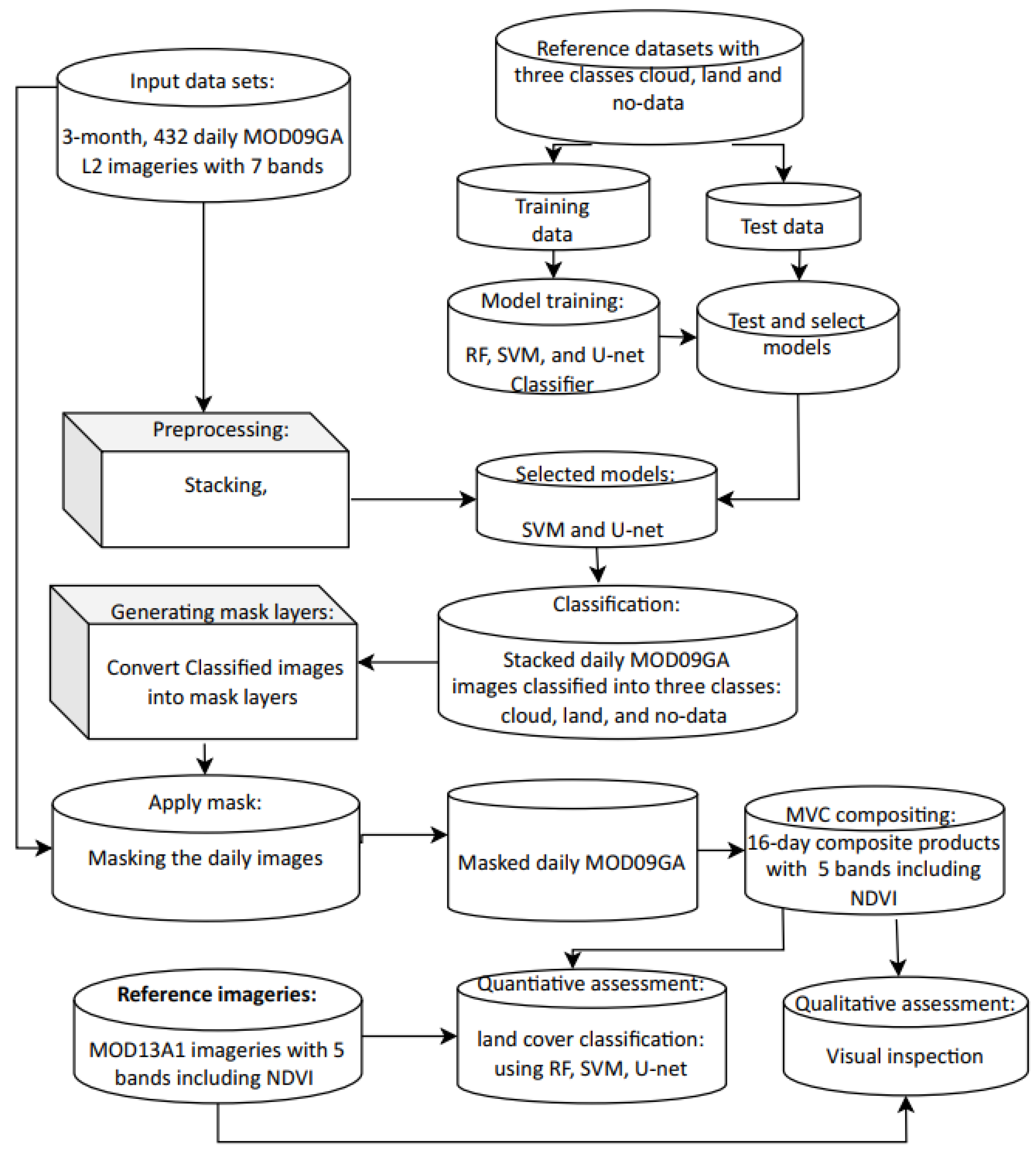
Hence, inspired by the existing limitations of the cloud-removal and pixel-based compositing approach, primarily related to the large spatial extent and multi-temporal data of high-temporal-resolution sensors, we propose a new single-rule-based compositing approach by generating our cloud mask. We employed maximum-value compositing techniques to derive 16-day MODIS composite products using daily MOD09GA Level 2 (L2) MODIS imageries, as shown in Figure 1. In order to mask cloud and no-data regions, we generated cloud mask layers from classified daily imageries by mapping the cloud-contaminated and no-data value pixels to −0.999999 and all uncontaminated pixels to 1. Then, the mask layers were utilized to mask the corresponding daily imageries by setting the masked pixels (cloudy and no-data) to −0.999999 while maintaining the original pixel values for the unmasked areas using the “np.where” function of the Python programming language. Subsequently, the masked imageries were composited by selecting the maximum value to generate 16-day MODIS composites for three seasons, for our target region covering Central, Eastern, and North Eastern Africa, and part of the Middle East, and requiring nine MODIS tiles to cover the area. Finally, we assessed the quality of our composite products quantitatively and qualitatively by comparing them with the reference MOD13A1v061 16-day composite products, which comprise an equal number of bands (5) as our products. Based on the land-cover classification accuracy, our products yielded a significantly higher accuracy (5–28%) than the reference MODIS product across three classifiers (RF, SVM, and U-Net), indicating the quality of our products and the effectiveness of our techniques. Moreover, a visual comparison shows that our products are more homogenous, radiometrically consistent, less noisy, and have fewer salt-and-pepper effects than the reference composite product.
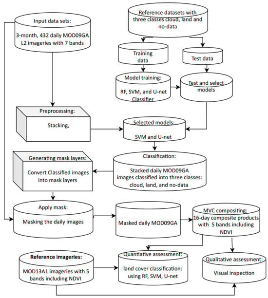
Figure 1.
Technical workflow.
Our method yields high-quality composite products for generating high-quality land-cover maps and investigating changes over time, essentially for extensive regions with persistent clouds and studies that require time-series data, such as land-cover mapping and change analysis, crop-type mapping, and phenological/seasonal variations. Moreover, the techniques can be applied for higher-resolution RS imageries regardless of the spatial extent, data volume, and type of clouds.
2. Materials and Methods
2.1. Selecting Region/Region of Interest
In order to conduct our experiments and collect the input MODIS imageries, we selected a region (see Figure 2), covering Central, Eastern, and North Eastern Africa, and part of the Middle East was selected. The region is characterized by a diverse range of climates, including tropical rainforests known for their persistent cloud cover, arid zones such as the Sahara, Sahelian, tropical, and equatorial climates, and various land-cover types such as forest, shrub, grassland, wetland, and bare land, and water bodies. The study area is selected not only because it includes regions with continuous cloud cover and rich biodiversity but also because it contains the second-largest tropical forest in the world, which plays a significant role in mitigating global climate change and environmental impacts. In addition, the existence of desert land and water bodies (lakes, seas, and oceans) in the region allows us to evaluate the effectiveness of our methods comprehensively. Owing to the extensiveness of the region, mosaicking nine tiles of MODIS images within h20v07 to h22v09, i.e., between horizontal (h) tile numbers 07–09 and vertical tile numbers (v) 20–22, is required to cover the entire area.
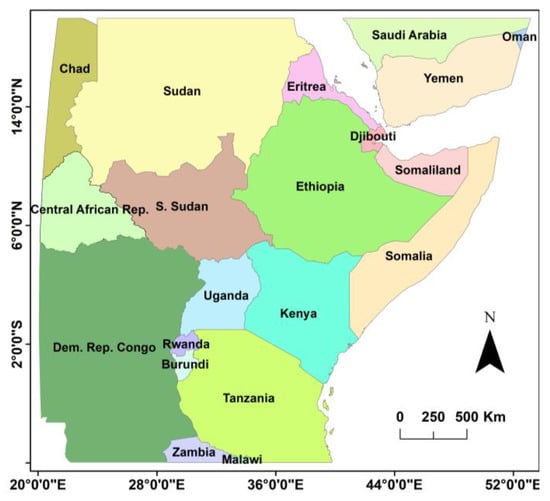
Figure 2.
Selected region for our experiment.
2.2. Datasets Description/MODIS Data Acquisition
We acquired two types of MODIS imageries, the MOD13A1 version (v) 061 Level 3 16-day composite product [47] for a reference dataset and the MOD09GAv061 Level 2 daily data [48] to generate our composite product, from the Earth data website: https://search.earthdata.nasa.gov, accessed on 26 April 2024. Level 2 data are atmospherically corrected surface reflectance data retrieved from Level 1 data, while L3 data are composited or averaged L2 products in sinusoidal projection [49]. MOD09GA is the primary input dataset for several MODIS land products [48], while MOD13A1 products provide reliable, geographic, and temporal time-series comparisons of global vegetation conditions, which provide valuable information for monitoring the terrestrial photosynthetic vegetation activity of the Earth, thereby facilitating research in phenology, change detection, and biophysical interpretations [50].
The imageries were captured during the same period within three seasons, specifically April–May 2019, July–August 2019, and January–February 2020. The time frame for the acquisitions of the imageries is purposefully selected so that the final composite products will be evaluated for land-cover classification using land-cover reference datasets collected within the specified period for our previous work [51].
As mentioned earlier, MOD13A1 datasets were utilized as reference datasets to acquire the corresponding daily Level 2 MOD09GA imageries (see Table 1), which were used to generate our composite products and assess their quality. A detailed description of the input imageries is given below.

Table 1.
Acquired MOD13A1v061 reference imageries with their cloud percentage and MOD09GAv061 input datasets.
2.2.1. Reference Composite Product: MOD13A1v061
MOD13A1v061 is a Level 3 global dataset. It is also known as the MODIS/Terra Vegetation Indices 16-Day L3 Global 500 m SIN Grid Product. The dataset comprises 16-day various composite products that include the Normalized Difference Vegetation Index (NDVI), Enhanced Vegetation Index (EVI), and four surface reflectance bands: Band 1 (red), Band 2 (near-infrared), Band 3 (blue), and Band 7 (mid-infrared). All products have a spatial resolution of 500 m and are projected in a sinusoidal (SIN) grid [47,50]. These composite images are generated by selecting the best pixels over 16 days based on low cloud, low view angle, and the highest NDVI/EVI value. The process primarily uses the Constrained View Angle–Maximum Value Composite (CV-MVC) techniques and at times employs MVC; otherwise, historical average data are considered if the best pixels are unavailable based on the two criteria [50]. To determine if the given pixel is cloud-free/uncontaminated, the MODIS cloud-masking algorithm employs spectral thresholding techniques [42].
For this study, 27 MOD13A1v061 scenes with 6 bands were downloaded, over three seasons, with most of the scenes having a maximum of 10% cloud cover. However, in a few cases where the 10% cloud content criteria were not met, scenes with higher cloud cover were acquired as indicated in Table 1. For this work, therefore, we extracted 5 bands such as the NDVI, Band 1 (red), Band 2 (near-infrared), Band 3, and Band 7 and stacked them using ENVI.
2.2.2. Input Imagery: MOD09GAv061
MOD09GA comprises Level 2 daily datasets consisting of seven surface reflectance bands, including Band 1, red (620–670 nm); Band 2, near-infrared (841–876 nm); Band 3, blue (459–479 nm); Band 4, green (545–565 nm); Band 5 (1230–1250 nm); Band 6, mid-infrared (1628–1652 nm); and Band 7, mid-infrared (2105–2155 nm), all with a 500 m spatial resolution. The datasets also include a quality assurance rating, observation coverage, observation number, and scan information in various spatial resolutions ranging from 250 m to 1 km.
To produce our 16-day composite imageries from MOD09GA and compare the result with MOD13A 16-day composite data, we downloaded 432 MOD09GA scenes with the 7 bands. In order to avoid results discrepancies due to the data acquisition and temporal compositing period, we selected the same period as MOD13A to acquire the daily MOD09GA imageries as elucidated in Table 1.
2.3. Hardware and Software
For this work, a laptop computer with a 2.7 GHz processor, 32 GB RAM, and an NVIDIA GeForce RTX 3050 Ti Laptop GPU (NVIDIA, Santa Clara, CA, USA), which has 4 GB dedicated memory and 16 GB shared memory, was employed. We utilized Python for data preprocessing, model training and evaluation, classification, and postprocessing. Python libraries/modules such as osgeo, gdal, ogr, glob, numpy, sklearn, TensorFlow, keras, pickle, matplotlib, geopands, and others were employed to perform the various tasks. In addition, ENVI 5.3 and Arcmap 10.3 were utilized for pre and postprocessing operations, including training data collection and ROI/shapefile manipulation, image stacking, and output visualization.
2.4. Collecting and Generating Reference Datasets for Cloud and Non-Cloud Classes
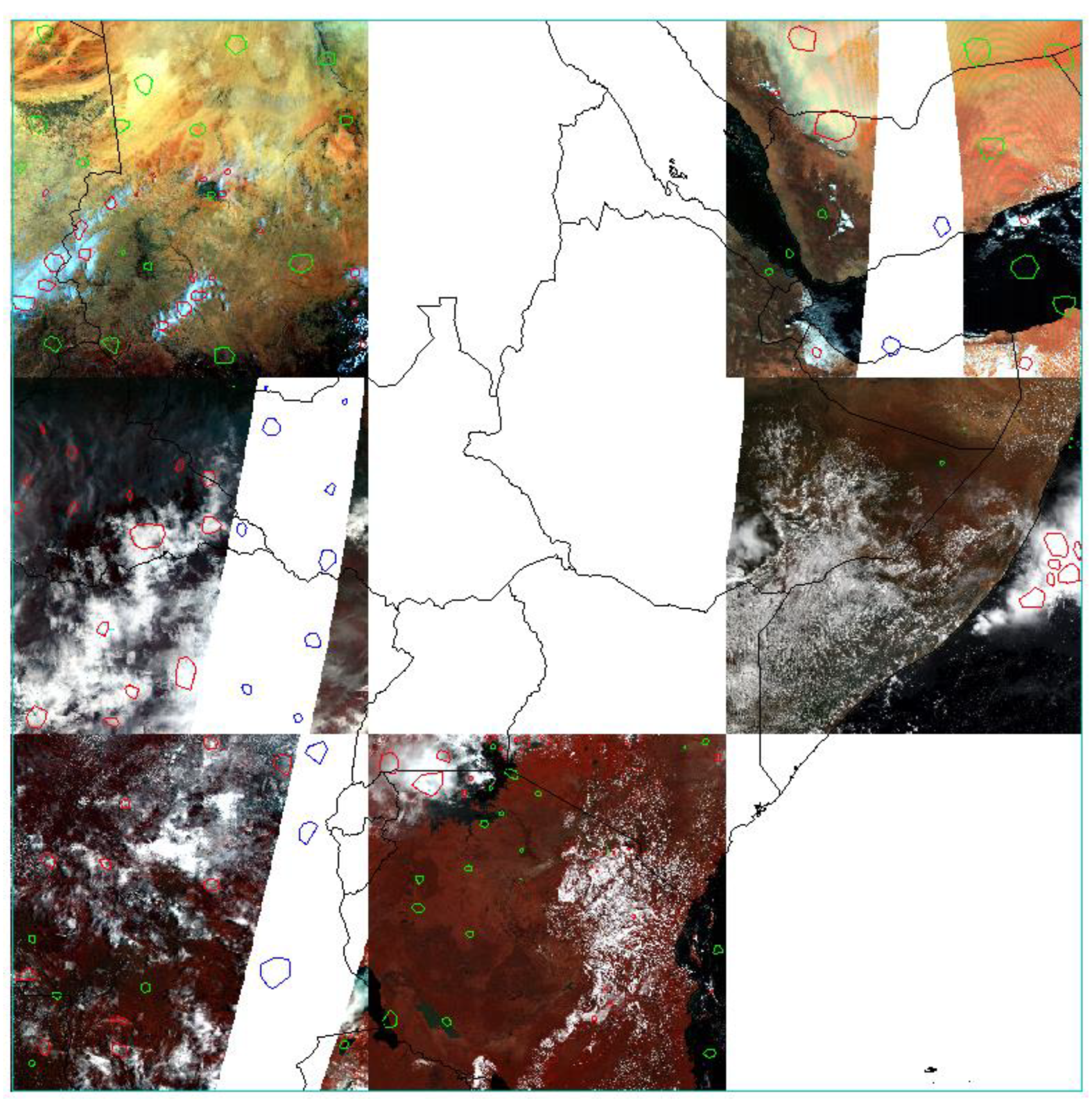
Employing sufficient representative reference datasets (training and tests) is one of the essential requirements for achieving the best result/accuracy in supervised classification [52,53]. Fortunately, obtaining cloudy and non-cloudy representative samples including missing values (no-data) is not challenging, unlike collecting examples for other supervised land-cover classification tasks. To collect sufficient reference datasets/labeled datasets, first, we selected MOD09GA daily imageries from different regions and seasons, then we annotated three classes including cloud, land (all non-cloudy pixels including water bodies), and no-data (pixels with missing values). The classes were annotated as a region of interest (ROI) and converted to shapefiles format using ENVI 5.3 software, as depicted in Figure 3. To effectively differentiate the various classes visually, we utilized true and false-color compositing techniques (see Figure 3). Specifically, false-color composites bands of (2, 4, 3), (1, 4, 3), (5, 3, 4), and (5, 3, 2) were utilized in most cases. In addition to their high spectral reflectance value, clouds are usually white and irregular in shape, appearing distinct in the scenes and making them identifiable visually mostly by employing false-color compositing of IR and the visible bands.

Figure 3.
Class labeling/annotation as a region of interest, cloud (in red), land (green), and no-data (blue) from selected MOD09GA daily imageries across different regions.
Once the labeled datasets were collected as shapefiles, the shapefiles were rasterized to create mask layers that comprise labeled and masked (unlabeled) pixels. Labeled pixels are the annotated regions or pixels enclosed by the polygons/ROI, with different values representing different class labels. Whereas, the masked pixels have zero values. After rasterization, the raster (r) is read as numpy arrays of 1D tensors consisting of [1, 2, 3, 0] that represent the three classes (cloud, land, and no-data) and the masked pixels, respectively. Then, the unlabeled pixels with zero values were excluded by applying basic logic (i.e., y = r [r > 0]), and only the labeled pixels with values of (1, 2, 3), which represent cloud, land, and no-data, were retained as a 1D tensor. Similarly, the corresponding input image (img), the base image from which the labeled data were obtained, was sliced using a simple operation, X = img [r > 0,:]. The slicing operation results in output datasets (X, y), where X represents the input image in the 2D tensor form, and y denotes the corresponding labels in 1D tensor/array format. Finally, the dataset (X, y) is saved as a numpy array. Using the same mechanisms and procedures, we collected several numpy arrays (X, y) from different MOD09GA imageries across the various regions and seasons to mitigate attribute variations in classes (land and cloud). In other words, the technique allows us to capture intra-class and/or interclass discrepancies that could occur due to variations in places and/or time. That means, collecting reference datasets across various seasons and regions allows us to detect spectral variations due to seasons or locations, which is essential to minimize/avoid misclassification of the same class into different classes or different classes into one category.
Finally, all the reference numpy arrays (X, y), generated from different MOD09GA imageries, were combined/appended to create representative training and test datasets for our models. Accordingly, we generated 981,255 training pixels, and 617,865 test pixels (see Table 2) from different scenes (see Figure 3). In addition, as pixel-based classifiers such as random forest (RF) and support vector machine (SVM) require different input formats then U-Net models, we reshaped the reference datasets/tensors to meet the models’ format requirements (see Table 2). Moreover, since we employ coarse resolution (500 m) imageries, we chose a smaller chip size (3 × 3) to minimize class heterogeneity that could compromise accuracy. In addition, using smaller chips helps us to address computational and memory expenses. For all operations described in this section, except the annotation/label data collection, all tasks were performed in Python 3.8.

Table 2.
Reference datasets of three classes (cloud, land, no-data).
2.5. Model Training and Evaluation
2.5.1. Model Training and Optimization
Previous studies have demonstrated that the type of classifiers/models employed plays a great role in achieving good results. In addition, the effectiveness of a model depends on the type, quantity, and quality of the reference and input datasets [53].
In this work, therefore, aiming to select the best classifiers, and to analyze the impact of classifiers on the final composite image, we employed three commonly used and robust machine-learning (ML) models: the RF, SVM, and U-Net.
Random forest (RF) is an ensemble classifier consisting of multiple decision trees, where each tree is built using randomly selected predictors from a subset of the training data and the final classification or prediction is determined by a majority vote [54,55,56]. SVM, on the other hand, is an algorithm that employs a separating hyperplane, which maximizes the distance between the nearest samples (i.e., the support vectors) to the plane, to separate different classes [53,57].
U-Net is a convolutional neural network (CNN) architecture commonly used for various image segmentation, including remote-sensing imageries. U-Net is named after its U-shaped design, which includes a series of convolutional and pooling layers followed by up-sampling and concatenation layers. U-Net is one of the most widely used semantic segmentation models owing to its efficiency in yielding a high accuracy [58,59,60,61,62]. The model comprises two paths: the convolution and deconvolution section/path. The convolution/contracting section is a sequence of convolutional and pooling layers that extract the contextual information. The deconvolutional/expanding path is the restoration or reconstruction path containing up-sampling and concatenation layers to combine low-level and high-level features and recover lost information during the encoding/convolutional stage, including spatial resolution and semantic details [60,63] and thereby allowing precise localization [64].
Thus, to select the best classifier among the three models, RF, SVM, and U-Net, we trained and evaluated the algorithms using the reference datasets presented in Table 2. While training the RF and SVM models, we employed default parameter values as given in the sklearn python library [65], but set the random state to zero. In addition, to run the SVM model in GPU so as to enhance the training and classification efficiency of the model, we employed cudf and cuML library [66] and executed the model in the Ubuntu terminal (Ubuntu 22.04.3 LTS), unlike the RF and U-Net that were run in the Spider Python console within the Windows environment.
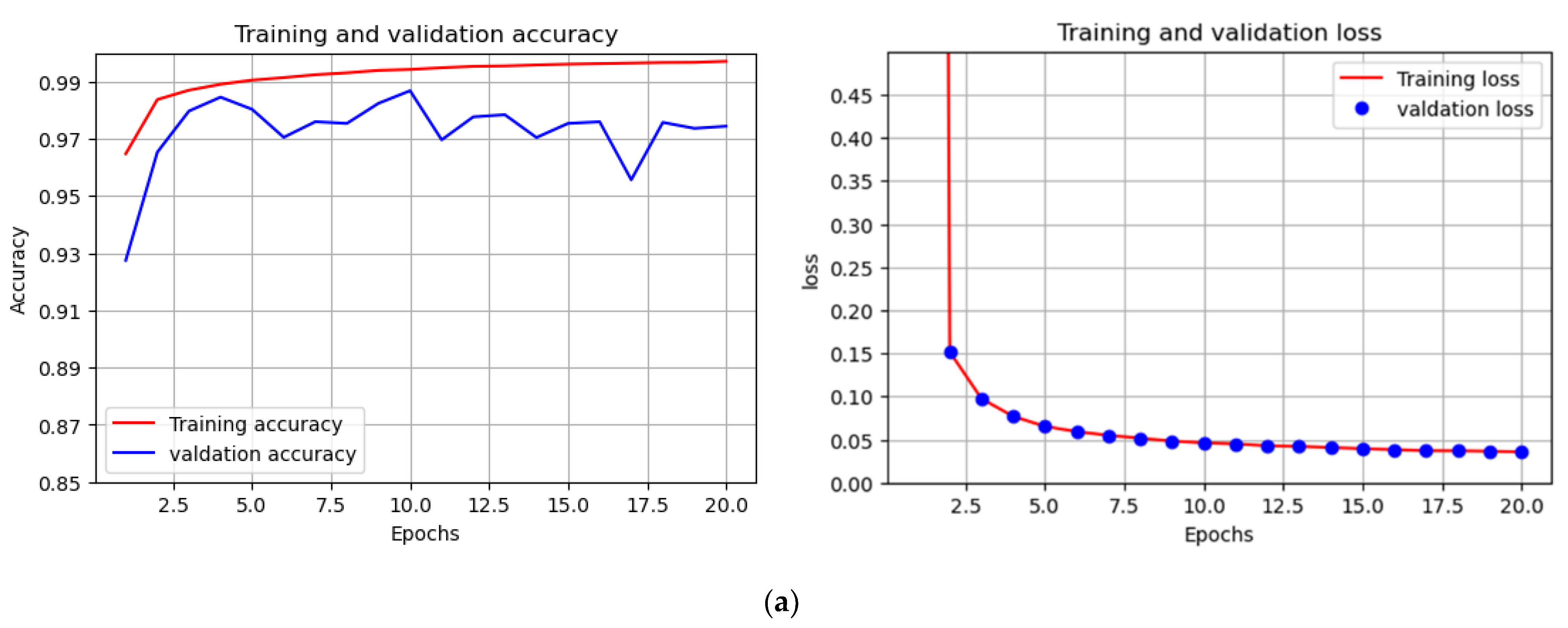
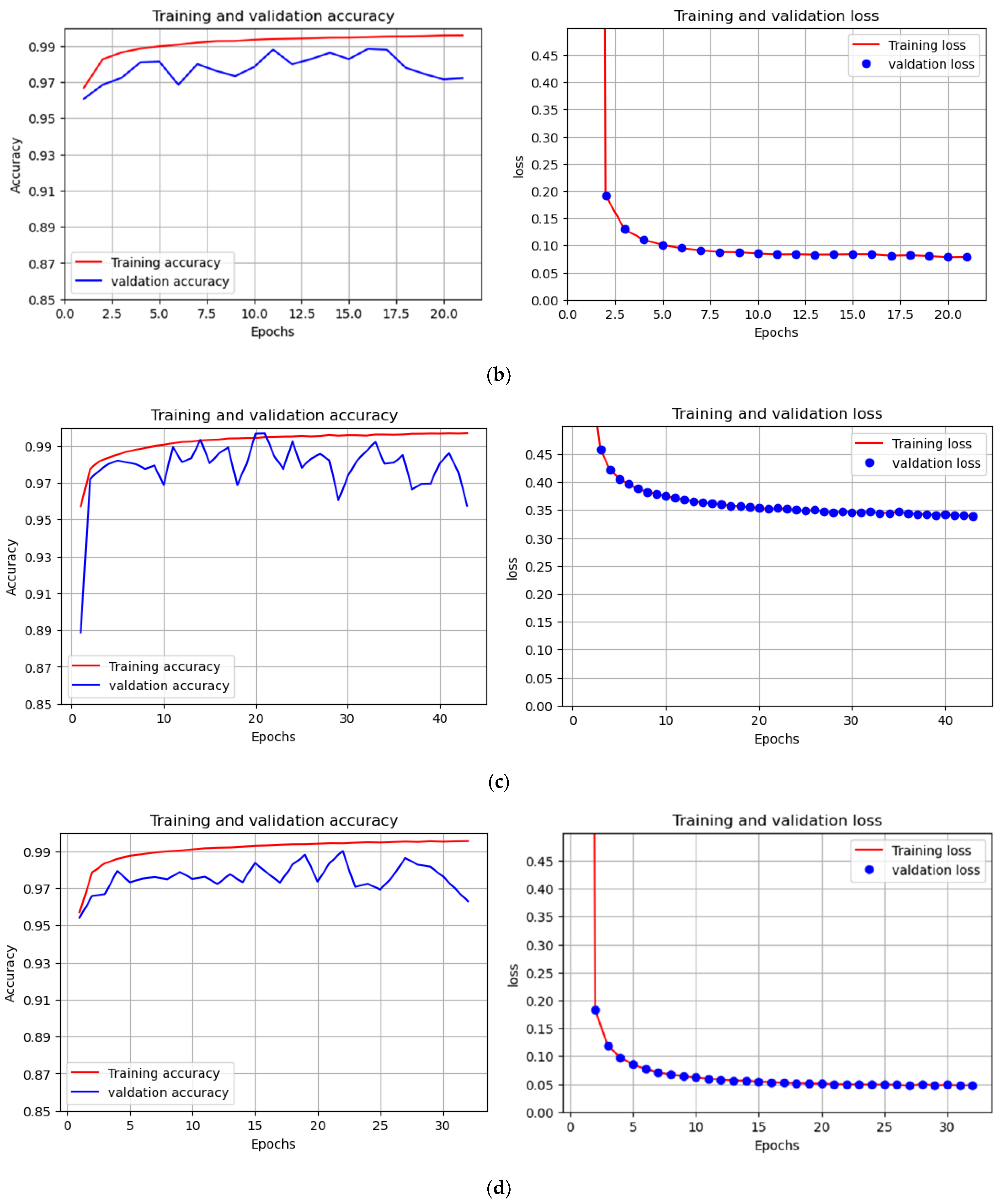
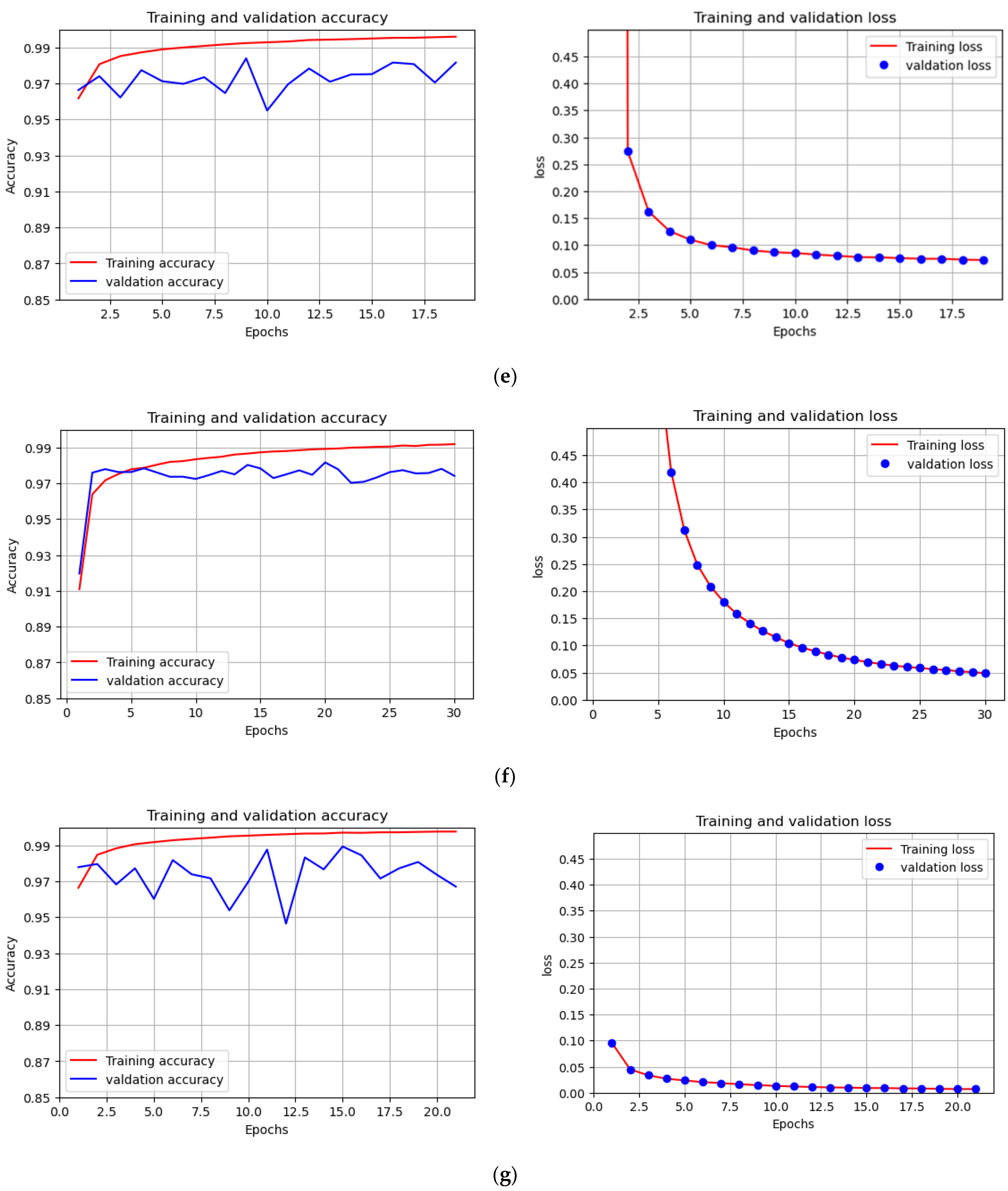
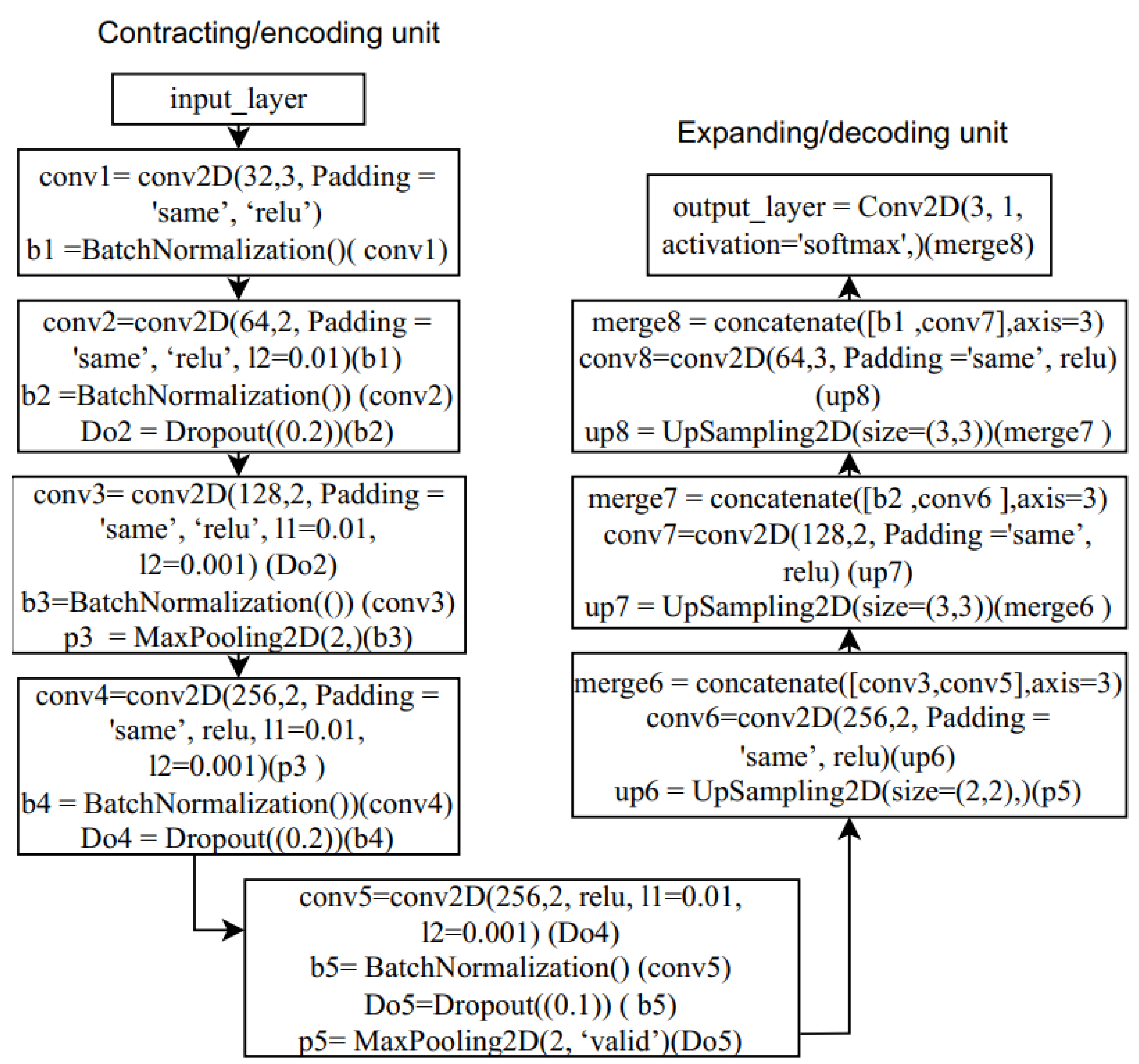
Regarding the U-Net segmentation model, we conducted several tests to obtain the optimum model by optimizing the various parameters such as weight and biases, and fine-tuning the hyperparameters (learning rate, batch size, number of epochs, number of hidden layers, and number of neurons in each layer). During experimentation, to control the learning process and avoid overfitting, we employed early stopping criteria with a patience of 10, which monitors validation losses, and we set the number of epochs to 150. In addition, to determine the number of convolutional layers in the encoding units, we experimented with U-Net models comprising 4, 5, and 6 CNN layers by setting the learning rate (0.0001) and a batch size of 32. Although the models achieve a similar overall accuracy (0.99) and k (98), they exhibit notable variations in their training and validation accuracy graphs, as well as in their training and validation loss graphs, as shown in Figure 4. Based on these graphs, we selected U-Net models with 5 convolutional layers (see Figure 5) as they demonstrated more stable/consistent training and validation accuracy graphs, and they appear to be the optimal model. This model is neither a little underfit as the model with 4 CNN layers is nor a little overfit as the one with 6 CNN layers is, which also has a higher loss.
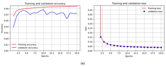
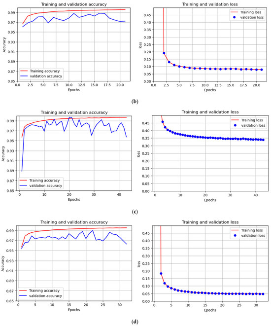
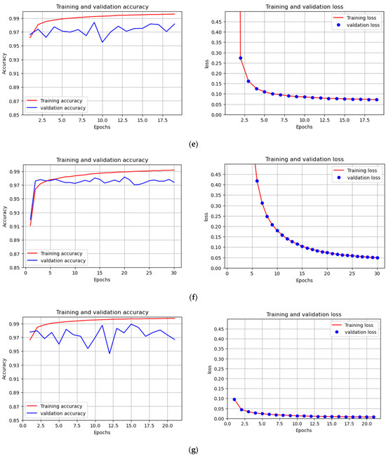
Figure 4.
Training and validation accuracy graphs, and their respective training and validation loss graphs, of various U-Net models. (a–c) Models with 4 CNN layers, 5 CNN layers, and 6 CNN layers, respectively, and a learning rate of 0.0001 and batch size of 32; (d) 5 CNN layer models, similar to Model b, but the number of filters in each layer is reduced by half; (e) Model similar to Model b, but a higher number of batches (64) were used; (f) 5 CNN layers as in Model b, but a lower learning rate (0.00001); (g) The model is the same as Model b with 5 CNN layers but without kernel regularization (L1 and L2).
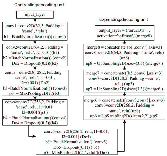
Figure 5.
Optimized U-Net architecture.
Once we obtained the optimum CNN layers/depth, we conducted further tests to fine-tune the model by varying the number of filters, batch size, and learning rates, as well as to see their impacts and the effect of kernel regularization (L1 and L2) (see Figure 4d–g). In terms of performance, the model showed no improvements; instead, it exhibited a varying degree of underfitting/instability. Therefore, the optimum U-Net model with 5 convolutional layers (see Figure 5) was chosen for the task.
2.5.2. Model Evaluation and Selection
As shown in Table 3, SVM and the U-Net models achieved the best results, overall accuracy (OA = 0.99), and kappa score (k = 0.98), while the RF achieved a 3% and 4% lower OA and k, respectively, than the two models. Consequently, the SVM and the U-Net model were selected to classify the MOD09GA L2 imageries.

Table 3.
Cloud non-cloud classification accuracy.
2.6. Classification and Masking
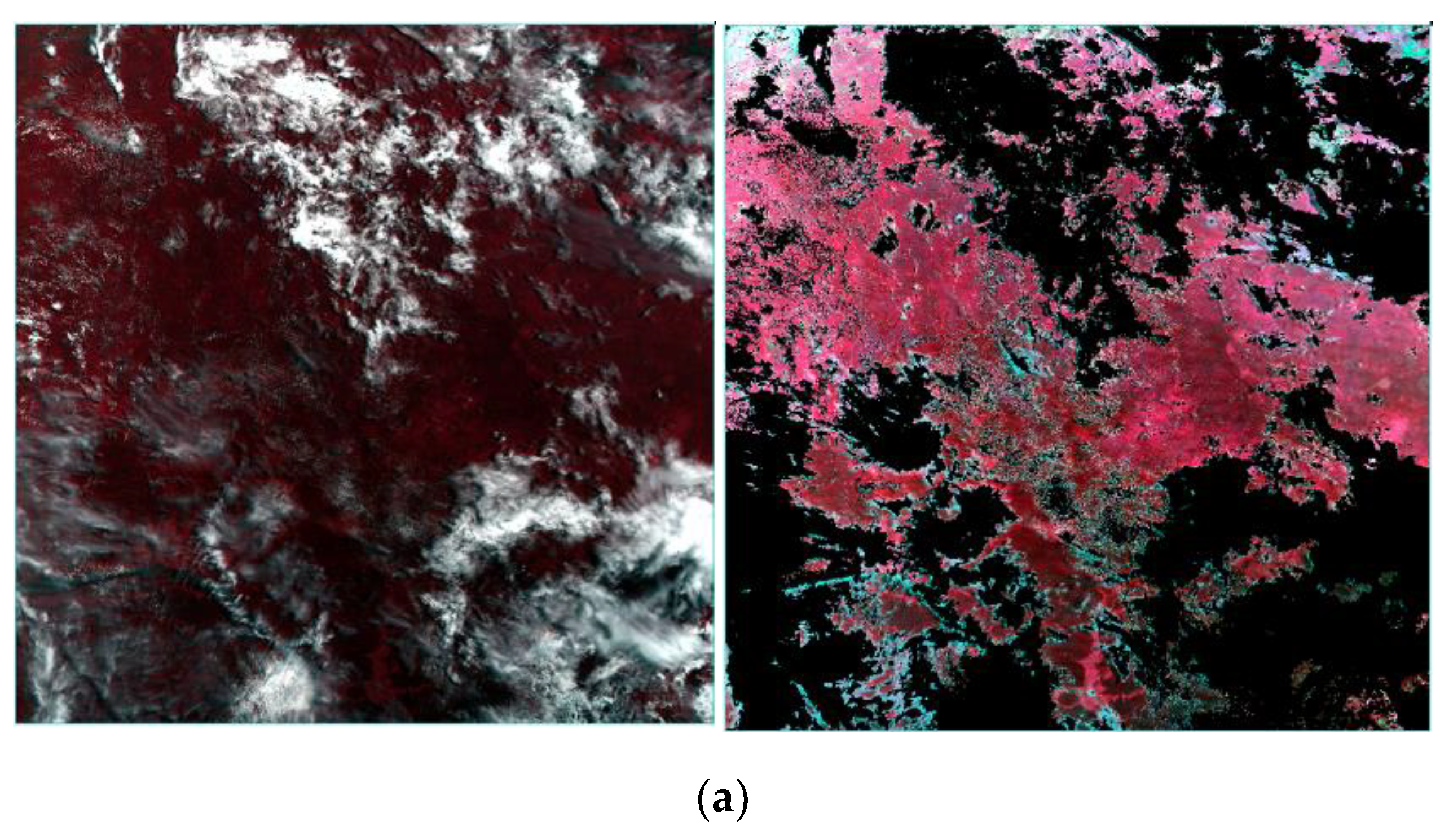
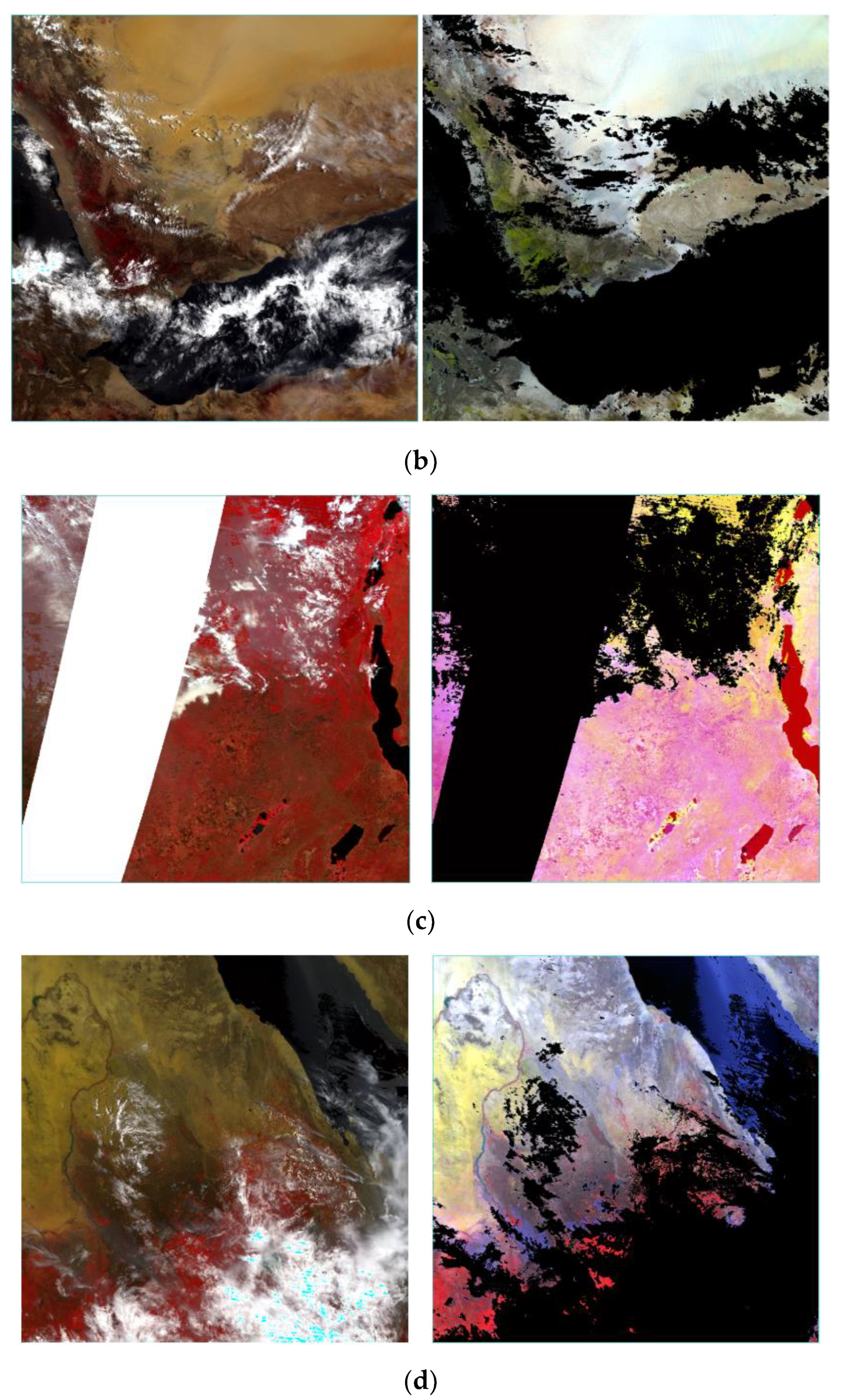
After selecting the SVM and U-Net models based on their performance, the models were employed to classify all (432) daily MOD09GA imageries with 7 bands. Then, each classified/predicted Tiff image was converted to a mask layer by altering the pixel values of the predicted image. In other words, we generated a mask layer from every classified/predicted image by changing their pixel values by employing value mapping. During value mapping, all pixels that were predicted as cloud (Class 1, pixel value = 1) were converted from 1 to −0.999999, pixels that were classified as land (Class 2, pixel value = 2) were changed from 2 to 1, and pixels that were predicted as a no-data value (Class 3, pixel value = 3) were set to −0.999999. In doing so, we successfully generated a mask layer with pixel values of −0.999999 for the cloud and no-data classes, and 1 for land, which comprises all uncloudy pixels including land and water bodies (see Figure 6).

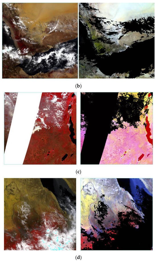
Figure 6.
Daily MOD09GA L2 imageries from various locations (Column 1) and their respective masked imageries (Column 2), clouds, and no-data pixels are masked. All imageries (a–d) but c of the 2nd column are false-color composites of NIR, red (Band 1), and green (Band 4). (a) MOD09GA.A2019197.h20v08.061.2020303164214.hdf and the corresponding masked image; (b) MOD09GA.A2019193.h22v07.061.2020303114043.hdf and the corresponding masked image; (c) MOD09GA.A2019207.h20v09.061.2020304034526.hdf and the corresponding masked image with false-color-composite of bands (5, 2, 1) to show water bodies which are not masked, (d) MOD09GA.A2019207.h21v07.061.2020304034241.hdf and the respective masked image.
Once the mask layer was generated, each mask layer/raster was used to mask its corresponding daily MOD09GA image/band in order to mask out the cloud-contaminated and no-data value pixels. To perform the masking, the function “np.where” was used to set the masked pixels to −0.999999 while keeping the original pixel values for the unmasked areas. In addition, during masking, we set the mask value to −0.999999 so that the value is distinct from land/target features’ actual surface reflectance values that range between 0 and 1. As a result, cloud and no-data values pixels in the daily MOD09GA images are effectively masked out as shown in Figure 6.
The whole procedure of creating mask layers and applying the mask was iteratively employed to generate two sets of masked daily images of MOD09GA. Each set corresponds to the classifier employed in deriving the mask layers, i.e., one set is derived from SVM-classified daily imageries and the other is generated from U-Net-classified imageries.
2.7. Pixel-Based Compositing
We employed a maximum value compositing approach to generate two sets of 16-day maximum value composite products (MaxComp-1 and MaxComp-2) from the two sets of masked daily MOD09GA imageries. MaxComp-1 products refers to the composite products generated from the masked images where the mask layers were derived from SVM-classified daily MOD09GA images. In contrast, MaxComp-2 refers to the composite products constructed from masked images where the mask layers were generated from U-Net-classified daily MOD09GA images, as described in Section 2.6.
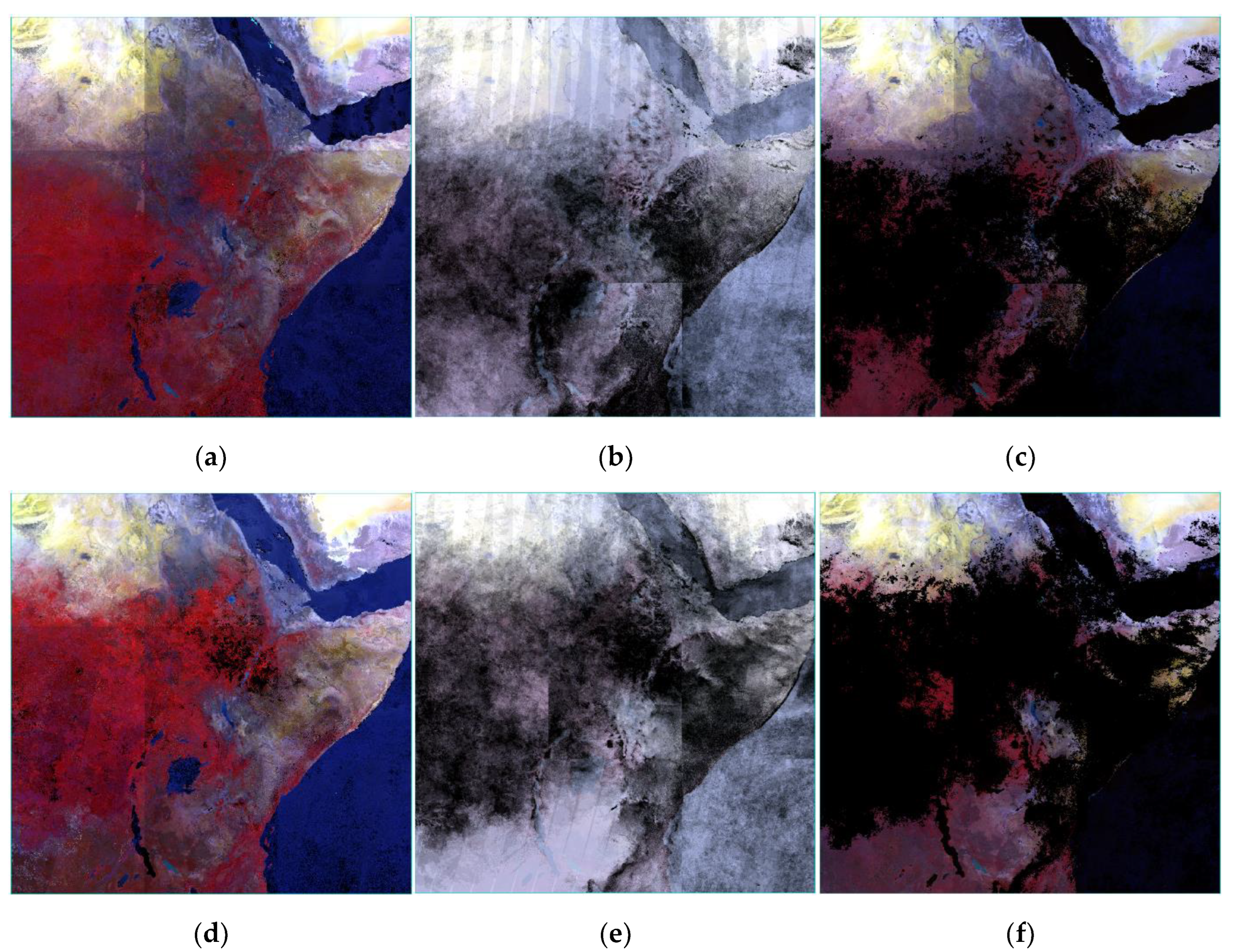
Concerning the compositing approach, the maximum value composite (MVC) technique was selected for two reasons. Firstly, the method allows us to choose the best pixels with the maximum reflectance value from the 16-day compositing period as the cloudy and no-data value pixels were masked out (assigned to a value of −0.999999), while other contaminated pixels or pixels under shadows exhibits lower reflectance values than their actual values. On the contrary, employing the common MVC-NDVI [6] or MAX-RNB [33] techniques will pick incorrect maximum values, particularly over certain land-cover features such as water bodies, shadow areas, and bare land if the pixels are cloudy or contaminated as the actual ratio could be smaller, which compromise the quality of the composite product. Secondly, utilizing either the mean or median compositing approach does not guarantee the best pixels in most cases. The mean compositing technique changes the reflectance value and other attributes of the image by averaging them; whereas, the median method computes the median values that can be any median values including the masked pixels if the region is under persistent cloud or shadow most of the time and/or if the majority of the pixels are contaminated. Moreover, the visual inspection of the three composite products indicates that the MVC method yields the best composite product (see Figure 7). Hence, we opted to employ the MVC technique to generate the two sets of maximum value composite images (MaxComp-1 and MaxComp-2) consisting of 4 non-derivative bands, Band 1 (red), Band 2 (NIR), Band 3 (blue), and Band 7 (mid-infrared), and MVC NDVI which was derived from the composited bands as described in Section 2.8.
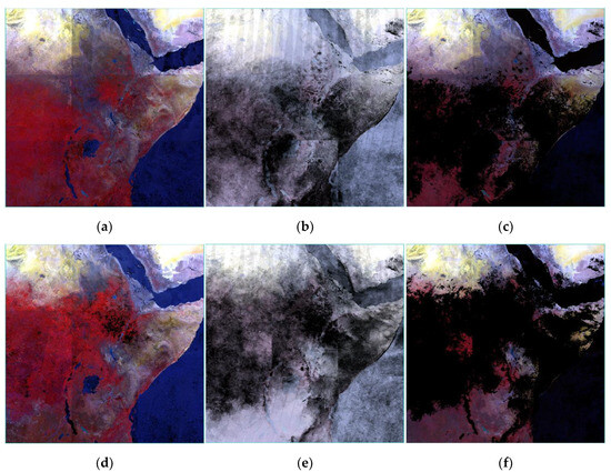
Figure 7.
Maximum-value, mean, and median composite products that were generated using imageries collected over two seasons, April–May (1st row), and July–August (2nd row). (a,d) MVC; (b,e) mean compositing; (c,f) median compositing. The products are presented as a false-color composite of Bands 2, 1, and 3.
2.8. MVC-NDVI Calculation
We computed 16 days of MVC-NDVI from the composited bands/images during the compositing process using Equation (1). During NDVI calculation, we replaced all positive and negative infinity values with zero to avoid unrealistic pixel values. The infinity values occur when the denominator in the NDVI formula is too small, i.e., the reflectance value of Band 1 and/or Band 2 is too small, and when the bands have the same mathematical signs, where Band 2 and Band 1 refer to NIR and red bands, respectively.
MVC-NDVI = ((MVC band 2 − MVC band 1)/((MVC band 2 + MVC band 1))
2.9. Band Selection
Since our reference composite product, MOD13A1, comprised five bands including Band 1 (red), Band 2 (NIR), Band 3 (blue), Band 7 (mid-infrared), and MVC-NDVI, we selected the same type and number of bands (5) for our composite products to ensure a fair comparison in terms of band type and quantity. Therefore, both of our composite products, MaxComp-1 and MaxComp-2, as well as the reference composite product (MOD13A1 16-day composite) comprise 5 bands for a single season and a total of 15 bands over the three selected seasons (April–May 2019, July–August 2019, and January–February 2020).
2.10. Assessing the Composite Products
To quantitatively evaluate the quality of our composite products (MaxComp-1 and MaxComp-2) for land-cover classification and compare their performance against NASA’s MOD13A1 16-day composite product, we selected three popular and effective machine learning classifiers, RF, SVM, and U-Net segmentation models. Then, the models were trained and assessed on the same label datasets (y), which comprise eight land-cover classes, while varying the input dataset (X) (see Table 4). While training the RF and SVM models, no parameter tuning was carried out; instead, we employed the default parameter as given in the sklearn library [65], as the main aim was to evaluate the quality of the input/composite datasets. In the case of the U-Net model, however, we utilized a similar model architecture as the U-Net model shown in Figure 5, but we adjusted the input tile size to 5 × 5 (see Table 4).

Table 4.
Reference datasets of 8 land-cover classes for training the models. Note: X varies depending on the input/composite image utilized, while y is the same label for the three models.
We selected the three models for two main reasons. Firstly, the quality of the input data is one of the most important parameters that impact the performance of the classifiers. Since different models apply different algorithms/mechanisms, their performance varies based on the properties or attributes of the input image such as the spatial resolution, presence of noisy pixels, mixed pixels, contaminations, and others. For instance, according to [57], the presence of noisy data/pixels in the input data significantly affects the accuracy of SVM as compared to other ML techniques. Therefore, using different types of classifiers enables us to analyze and understand the properties and quality of the input datasets across different algorithms. Otherwise, the effect of the input datasets may be less noticeable and understood if we rely on only a single classifier. The other reason is that utilizing different models to assess the land-cover classification accuracy produced from different input datasets allows us to evaluate the consistency of the classification results across the different models and input datasets.
In addition to quantitative evaluation, we employed a qualitative assessment mechanism, where we compared our product with the reference MOD13A1 16-day composite provided by NASA via the visual inspection technique.
3. Results
3.1. Land-Cover Classification Accuracy
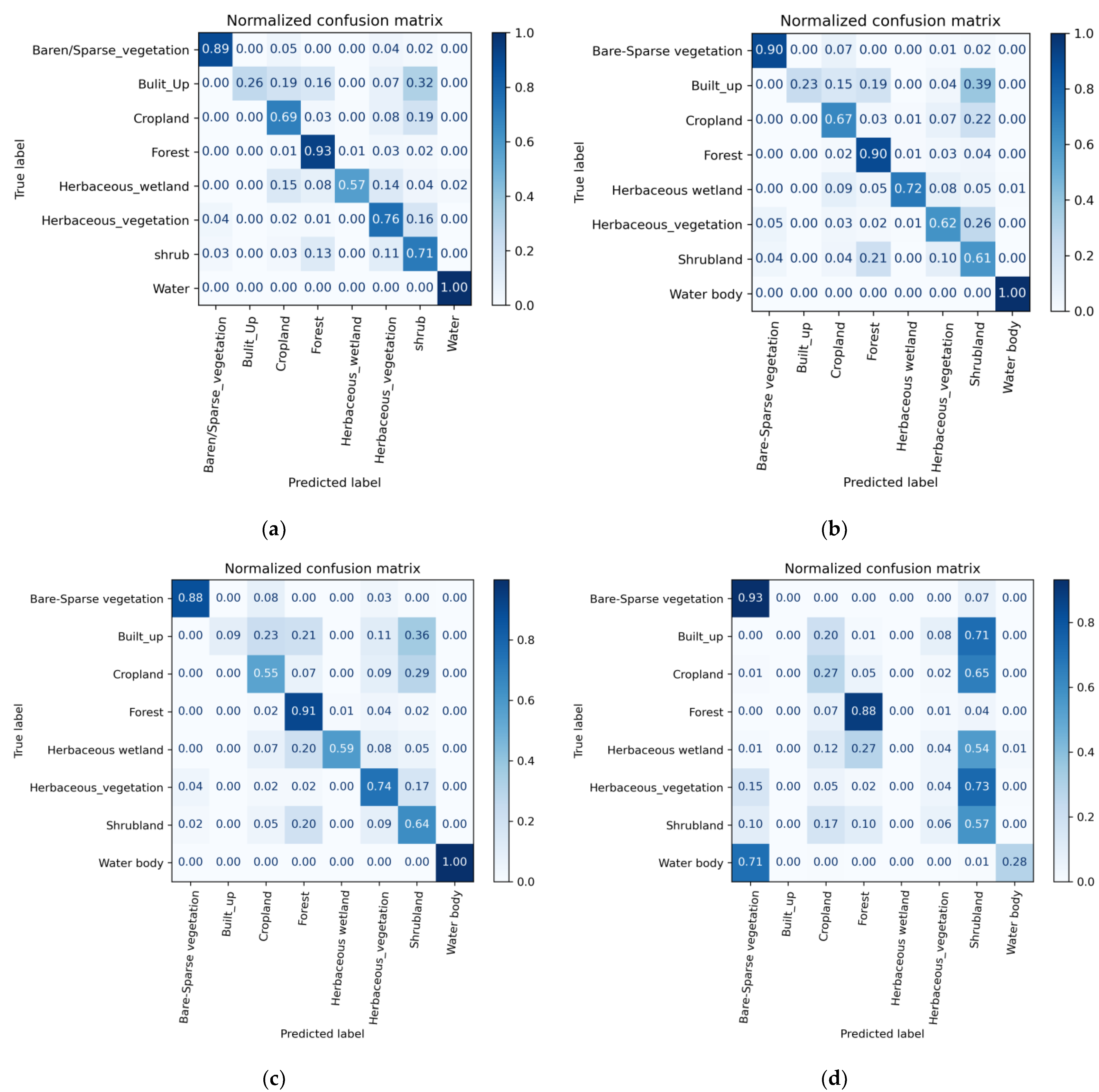
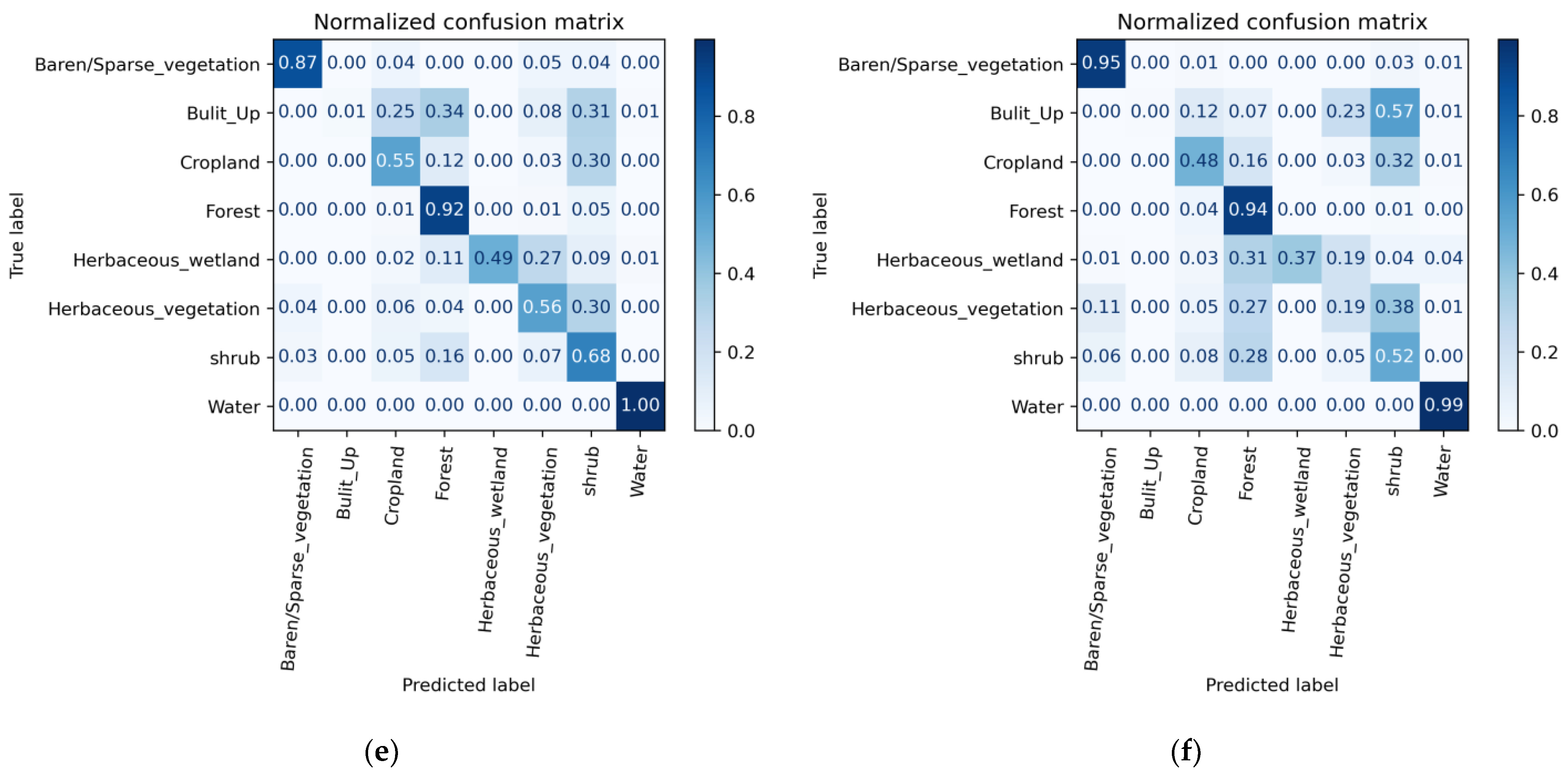
As shown in Table 5 and Figure 8, the land-cover classification results from the three different classifiers indicated that our composite products, MaxComp-1 and MaxComp-2, achieved a significantly higher accuracy (5–28%) than the reference MOD13A1 16-day composite product. While both of our products outperformed the reference composite product across all classifiers, significant accuracy discrepancies exist within the same classifier and among the three different classifiers, suggesting differences in the quality and/or characteristics of the input datasets and classifiers.

Table 5.
Land-cover classification performance of our composite products and the reference composite product (MOD13A1) on three models.

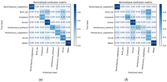
Figure 8.
Confusion matrices depicting the performance of our best composite product (MaxComp-1) (1st column) and the reference composite product (MOD13A1) (2nd column) across three different classifiers. (a) Input: MaxComp-1, Model: RF; (b) Input: MOD13A1, Model: RF; (c) Input: MaxComp-1, Model: SVM; (d) Input: MOD13A1, Model: SVM; (e) Input: MaxComp-1, Model: U-Net; (f) Input: MOD13A1, Model: U-Net.
When RF classifiers were applied, our composite products (MaxComp-1 and MaxComp-2) achieved the highest accuracy (OA) of 0.80 and a kappa coefficient/score (k) of 0.76, which are 5% and 6% higher OA and k values than the best accuracy achieved by the reference product, respectively.
However, significant performance discrepancies were noted among the products when SVM classifiers were utilized. MaxComp-1 achieved an OA of 0.75 and a k of 0.70, which are 28% and 34% higher than the OA and k values of the reference composite data, respectively, while MaxComp-2 attained an OA and a k 16% and 19% lower than the OA and k of MaxComp-1, respectively. Similarly, when the U-Net model was employed, MaxComp-1 outperformed both MaxComp-2 and the reference composite data, although the accuracy variations were not as significant as when SVM was utilized. MaxComp-1 attained an OA = 0.73 and k = 0.68, which are 8% and 11% higher than the OA and k of the reference composite data, and 3% and 5% higher than the OA and k of MaxComp-2, respectively.
The results indicate that MaxComp-1 achieved the highest classification accuracy across all three classifiers, highlighting the quality of the product.
3.2. Visual Inspection
The visual inspections of the composite imageries across the three seasons reinforce the quantitative evaluation. As depicted in Figure 9, MaxComp-1 composite images are more homogeneous, i.e., less noisy, which is seen clearly when zoomed in, compared to MaxComp-2 and the reference composite products. On the contrary, MaxComp-2 and the reference composite products exhibit notable heterogeneity, due to the prevalence of noisy pixels and, in some places, to salt-and-pepper effects (see Figure 9b,c,e,f,h,i).
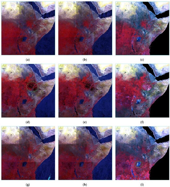
Figure 9.
False-color composite of our composite products and the reference composite product (MOD13A) across three seasons: April–May 2019, 1st row; July–August 2019, 2nd row; January–February 2020, 3rd row. (a,d,g) MaxComp-1 products; (b,e,h) MaxComp-2 products; (c,f,i) MOD13A1v061 L3 products (reference composite products). The green circle highlights the main difference between our composite product and the reference data.
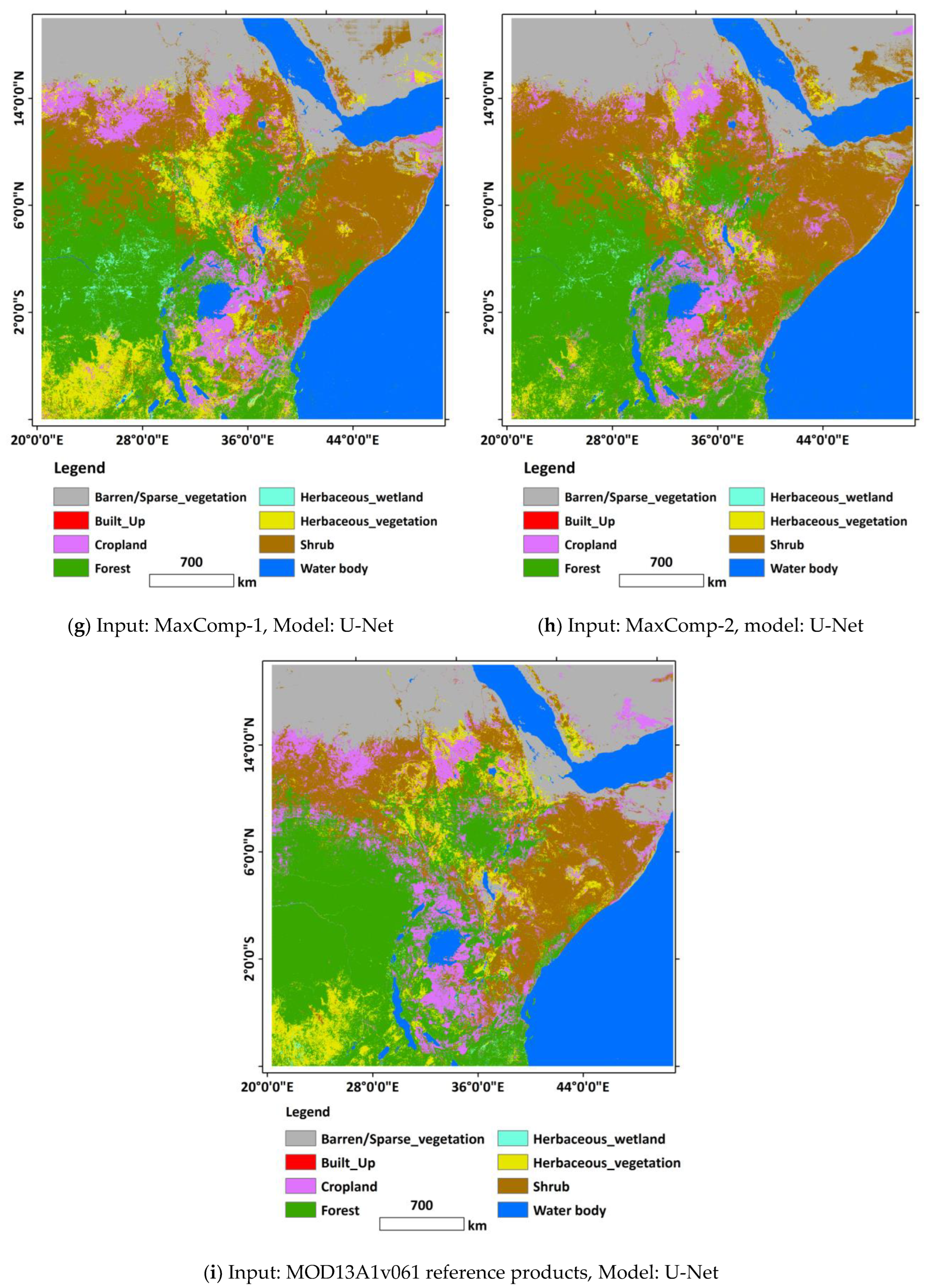
Furthermore, the variations in the quality of the input datasets are manifested in the land-cover maps generated by the same classifiers as Figure 10 elucidates. For instance, when MaxComp-1 was used as an input, the three classifiers (RF, SVM, and U-Net) generated land-cover maps revealing minor variations (see Figure 10a,d,g) in which all eight classes were predicted. However, land-cover maps generated from MaxComp-2 and the reference composite product (MOD13A1) show remarkable discrepancies across the classifiers, including missing classes (see Figure 10b,c,e,f,h,i). In particular, when the SVM classifier was employed to classify MaxComp-2, only seven classes were predicted out of eight, and one class (water body) was misclassified as bare–sparse vegetation (see Figure 10e). Likewise, when the reference composite product (MOD13A1) was classified using the SVM model, only six classes were predicted out of eight, while two classes (built-up, and herbaceous wetland) were completely missed (see Figure 10f).
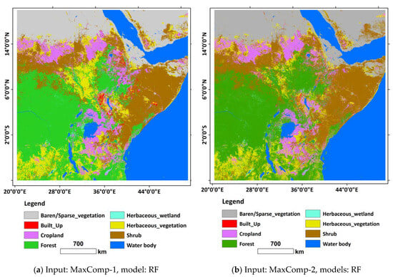
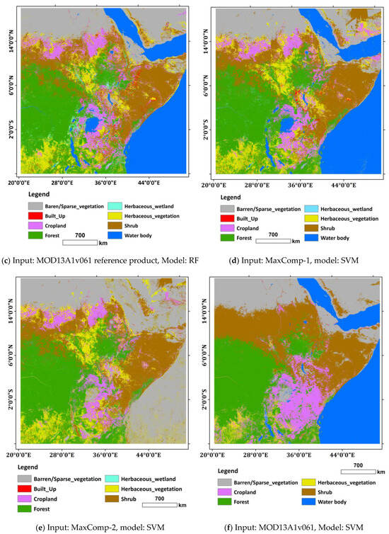

Figure 10.
Land-cover maps generated using our composite products (MaxComp-1 and MaxComp-2) and the reference composite product (MOD13A) by employing three different algorithms (a–i).
4. Discussion
As described in Section 2.10 and Section 3, quantitative and qualitative methods were employed to assess the quality of our composite products and the compositing technique. To quantitatively evaluate the products, we performed the land-cover classification of eight classes using our composite products and employing three different ML models (RF, SVM, and U-Net). Subsequently, we compared the classification accuracies with that of the reference composite product (MOD13A1).
Table 5 and Figure 8 reveal our composite products consistently yielded the best classification accuracy compared to the reference composite product (MOD13A1) across the three classifiers. However, the results show significant accuracy variations (5–28%). The maximum accuracy discrepancies were observed between MaxComp-1 and the reference data MODIS composite when the same SVM classifier was employed. MaxComp-1 achieved an OA of 0.75 and a k of 0.70, which are 28% and 34% higher than the OA and k attained by processing the reference composite product, respectively. On the other hand, the least accuracy difference (5%) between the two products was noted when the RF model was employed, where MaxComp-1 yielded the best accuracy of 0.80 OA and 0.75 k, which is 5% higher than the accuracy achieved when the reference composite dataset was manipulated.
The results demonstrated that our techniques yielded better-quality composite products than the MODIS-provided L3 MOD13A1 products. In other words, our approach generated higher-quality, cleaner imageries by removing/masking out more clouds, shadows, and noise than the MODIS approach.
Moreover, visual inspection and comparison of the products (see Figure 9) reveals that our products exhibit less heterogeneity and smoother appearances than the reference composite imageries. This implies the effective removal of clouds/noises and reaffirms the quantitative results. In particular, MaxComp-1 products appear more homogeneous, with lesser noise or artifacts, including white spots and patches (unmasked/removed cloud), than the MaxComp-2 and the reference MODIS composite images.
4.1. Role of Classifiers
Supervised classification is the most integral tool in our compositing approach, essentially in generating mask layers and evaluating the quality of the composite products. As mentioned earlier, we employed three classifiers, RF, SVM, and U-Net models, for our work. These classifiers are fundamentally different in their mathematical principles and core concepts, the structure of the algorithms and/or model architectures, the methods they employ to perform classifications, and the type of information they utilize to categorize different classes. Consequently, the performance of these classifiers significantly depends on the type and quality of input datasets and the properties of the classifiers.
As shown in Table 5 and Figure 8, considerable accuracy discrepancies are observed across the three classifiers. These variations can be classified into two based on the factors causing the discrepancies. The first type of discrepancy arose when we varied the input datasets while applying the same type of model; whereas, the second type occurred due to variation in the classifiers while using the same input datasets.
In the first case, when we kept the model constant and varied the inputs we found that each classifier achieved its best accuracy when the MaxComp-1 input was utilized. For instance, when the RF model was used, MaxComp-1 attained the best results (OA = 80%), 5% higher than the reference MODIS product. However, when the SVM classifier was employed the highest discrepancies were observed. Using the SVM model, MaxComp-1 achieved an OA of 0.75 and a k of 0.70, which are 28% and 34%, and 16% and 19%, higher OA and k values than those of the reference MODIS product and MaxComp-2, respectively. Moreover, the two products, the reference MODIS product and MaxComp-2, yielded the lowest and second lowest kappa, 0.36 and 0.51, respectively. This indicates the two datasets contain more contaminated pixels and are noisier and more heterogeneous as compared to MaxComp-1. In addition, the heterogeneity of the products is manifested in the land-cover maps as shown in Figure 10e,f, where the water bodies are misclassified as bare–sparse vegetation. Furthermore, when the U-Net was employed, the MaxComp-1 attained a higher accuracy; OA = 0.73 and k = 0.68, which are 8% and 11% higher than the result achieved by the reference composite product, and 3% and 5% higher than the OA and k achieved by MaxComp-2, respectively. Overall, the results demonstrated that Maxcomp-1 is the best composite product with fewer contaminated pixels.
The other type of accuracy discrepancy occurred when the classifiers were varied while the inputs were the same. In this scenario, the performance of the classifiers varies substantially despite using the same input datasets. In other words, it is a discrepancy due to the characteristics of the classifiers and input datasets. For example, the accuracy difference between the RF model and SVM when MaxComp-1 was processed is 5%. However, the highest (28%) and the second highest (21%) variations were noted when the MOD13A1 product and the MaxComp-2 were manipulated, respectively. This indicates that the SVM model is highly impacted by the heterogeneity of the input datasets as compared to RF and U-Net, which further implies the quality of the input datasets. In particular, achieving the lowest and the second lowest accuracy and kappa by employing SVM with the reference composite (MOD13A1) and MaxComp-2, respectively, suggests the heterogeneity of the composite products. This heterogeneity arose from the presence of contaminated pixels that were left unremoved by the compositing techniques. In agreement with our observation, Foody and Mathur [57] noted that the SVM classifier is highly impacted by noisy pixels in the image. Moreover, according to [67], differences in kappa values while using the same classifier with different inputs indicate the quality of input imageries, where the lowest k infers the lowest quality input dataset.
Furthermore, obtaining the best quality composite product (MaxComp-1) using cloud mask layers derived from SVM-classified daily MOD09GA images implies that SVM is the best model for cloud mask generation. In other words, the classifier is more effective than RF and U-Net for classifying cloud, land (uncloudy pixels), and no-data pixels. That is most likely due to the nature and number of classes that suit the model’s property. In our case, the number of classes is mostly two (cloud, land). However, when the images consist of no-data pixels, the number of classes becomes three that have distinct attributes. This situation, having a small number of classes with easily separable attributes, suits SVM’s inherent property. In other words, since the algorithm was originally developed for two-class separation [53,68,69,70], it achieves the best results when the classes possess distinct attributes or exhibit notable variations [57,68]. Moreover, SVM attains high accuracy and generalizes well using small training data [69] as it requires only a few samples to draw an optimum boundary between classes unlike any other ML algorithms [53,68]. Furthermore, the algorithm does not use all the training samples to construct classification boundaries; instead, it uses a few samples (support vectors), a subset of the training set, to find the optimum separating plane, making it less prone to overfitting [68]. That could explain why SVM outperformed the two classifiers (RF and U-Net) in classifying cloud, land (uncloudy pixels), and no-data pixels for generating cloud masks.
On the other hand, as opposed to several previous findings (e.g., Solórzano et al. [58], Heydari and Mountrakis [71], and Stoian et al. [72]), the U-Net DL model, which employs both spatial and spectral information for class separation [58,71,73], did not yield the best classification accuracy in both cloud and land-cover classification. This implies that spatial resolution has little significance in coarse-resolution imageries as pointed out by [74,75,76].
Overall, the results indicate the quality of the final composite product is strongly associated with the quality of the mask layers. In other words, the type of classifier employed plays a great role in determining the quality of the mask layer and the quality of the final composite product.
4.2. Comparison with Previous Works and Recommendations
Our maximum-value compositing algorithm selects pixels with the highest reflectance values from the candidate pixels for each band unlike the previous MVC technique [6,35,50], which depends on the maximum NDVI values to pick the best pixels for compositing. Moreover, our algorithm not only screens the masked cloudy pixels but also removes clouds, noise, and contaminated pixels, provided that the clouds are effectively masked and at least one uncontaminated pixel is available from the candidate pixels. In other words, the quality of our composite products relies on the efficiency of the classifier selected to classify the daily images from which the cloud mask layers were derived. Hence, selecting an appropriate classifier and acquiring sufficient representative reference samples for the various cloud types (thick cloud/haze, thin cloud) and uncloudy pixels is critical to generating effective cloud mask layers.
Moreover, most of the existing composing techniques are specific to particular types of sensors that employ specific cloud masks. For instance, BAP, PAC, MAX-RNB, WPS, MEDOID, and NLCD were developed using Landsat imageries and cloud masks generated using the Function of Mask (Fmask) algorithm [40], which has its own limitations [38] in terms of detecting thin clouds, cloud edges [28], and shadows [36]. Before the development of the Fmask algorithm, supervised classification methods, particularly decision tree algorithms, had been applied to create cloud masks for Landsat image composing by employing different compositing mechanisms (e.g., Potapov et al. [34], Roy et al. [35], and Hansen et al. [41]). On the other hand, low- and medium-resolution imageries, such as AVHRR and MODIS, employ cloud masks created based on thresholding mechanisms on various spectral bands [42,43,44]. However, the thresholding approach has never been global as commission and/or omission errors are common [45,46], especially around the threshold limit where the degree of confidence in cloud detection is low [42].
4.3. Recommendations
Although our approach can yield a high-quality composite product, the quality of the product hugely depends on the type of classifiers, as well as representative reference datasets (cloud, land (all non-cloudy pixels), and no-data classes).
Regarding the classifier, for coarse- and medium-resolution imageries we recommend using the SVM algorithm not only because of its performance in classifying cloud and no-cloud pixels but also due to its inherent ability to separate a few classes with distinct attributes. However, for higher-resolution imageries, where spatial information is crucial, exploring different advanced DL methods is recommended along with SVM to obtain the best cloud mask. In our case, the DL technique, U-Net was outperformed by SVM in classifying cloud and non-cloud pixels, suggesting the insignificance of spatial information in coarse-resolution image classification.
Concerning the datasets, it is crucial to employ sufficient and representative training datasets and input imageries comprising multi-spectral bands including NIR and MIR. Provided that these conditions are met, our method can be effectively implemented for any remote-sensing imageries regardless of their spatial resolutions, data sizes, study area extents, and cloud conditions/types. Moreover, this approach does not require a specific masking algorithm and auxiliary data. However, although our study considered an extensive region with a range of climates and land-cover features, testing the methods in the more climatically diverse and larger area, including the polar regions, will aid in comprehensively evaluating our method.
5. Conclusions
This study presented an alternative satellite image compositing strategy to circumvent the challenge of obtaining cloud-free scenes, especially for extensive areas known for persistent cloud cover. Fundamentally, our approach differs from the existing compositing technique by which cloud mask layers are generated. We systematically selected a large study area that includes Central, Eastern, and Northern Africa, and part of the Middle East. This region is characterized by diverse climatic conditions including the tropical rainforests known for persistent cloud cover, arid/desert climates, and equatorial climates, as well as various land-cover features. Then, we acquired a total of 432 MOD09GA L2 daily MODIS datasets, comprising seven bands, over three seasons. Subsequently, we collected representative reference samples (training and test datasets) with three classes: cloud, land (all uncontaminated pixels), and no-data. Using these reference samples, three robust ML classifiers, RF, SVM, and U-Net, were trained and tested to select the best classifier and assess the impact of the algorithm on the final composite product. Consequently, SVM and U-Net were selected and employed to classify all the daily images and generate two sets of classified rasters. Then, the classified rasters were converted into cloud mask layers by mapping the cloud and no-data pixels’ values to −0.999999. Subsequently, the mask layers were used to mask the corresponding MODIS daily images by employing the special function “np.where” in Python. This resulted in masked images where pixels have a value of −0.999999 if they are masked out, indicating a cloudy/no-data value; otherwise, the pixels retain their actual reflectance values.
After masking out the cloud and no-data pixels, we generated 16-day composite products using three approaches, the maximum-value, median-value, and mean-value methods. Subsequently, we visually compared the products to select the best technique. Comparisons of these products revealed that the maximum value method yielded the best products. Consequently, we employed the technique to generate two sets of maximum-value composite products, MaxComp-1 and MaxComp-2, associated with the two sets of cloud mask layers generated using the SVM and U-Net models, respectively.
Finally, we assessed the quality of our products both quantitatively (for land-cover classification) and qualitatively (through visual inspection) and compared the results with the MOD13A1v061 L3 16-day composite product provided by NASA. In order to make the comparison fair, we made the comparison with all the products comprising the same types and number (5) of bands, MVC-NDVI, Band 1 (red), Band 2 (near-infrared), Band 3 (blue), and Band 7 (MIR), that were acquired during the same period.
Accordingly, we present the following:
- Our composite products yielded the best classification accuracy across three classifiers, RF, SVM, and U-Net.
- Our technique is more effective in removing clouds, noise, and contaminated pixels than the methods used to produce the MOD13A1v061 L3 16-day composite product.
- The MaxComp-1 product yielded the best classification results across the three classifiers with the fewest accuracy discrepancies.
- The highest variation (11%) between OA and the kappa score, and the lowest k (36%), were observed when manipulating the reference MOD13A1 using SVM, and the second lowest k (51%) was observed when MaxComp-2 was processed. These discrepancies in accuracy strongly suggest the two products are more heterogeneous comprising more contaminated pixels than MaxComp-1.
- The MaxComp-1 product is more consistent both spectrally and radiometrically, and less noisy, with fewer salt-and-pepper effects.
- SVM is the best model for cloud mask generation, i.e., in classifying cloud, land (non-contaminated pixels), and no-data pixels compared to RF and U-Net.
Author Contributions
Conceptualization, T.A., W.X. and J.F.; Data curation, T.A. and J.F.; Formal analysis, T.A.; Investigation, T.A.; Methodology, T.A.; Software, T.A.; Project administration, T.A., W.X. and J.F.; Resources, T.A., W.X., J.F., H.J. and X.L.; Supervision, W.X. and J.F.; Validation, T.A., W.X., J.F., H.J. and X.L.; Visualization, T.A., W.X., J.F., H.J. and X.L.; Writing—original draft, T.A.; Writing—review and editing, T.A. All authors have read and agreed to the published version of the manuscript.
Funding
This work was supported by the National Key R&D Program (2021YFE0117400).
Data Availability Statement
MODIS imageries, the MOD13A1 version (v) 061 Level 3 16-day composite product, and the MOD09GAv061 Level 2 daily data can be accessed for free from the Earth data website: https://search.earthdata.nasa.gov, accessed on 26 April 2024.
Conflicts of Interest
The authors declare no conflicts of interest.
References
- Wulder, M.A.; Roy, D.P.; Radeloff, V.C.; Loveland, T.R.; Anderson, M.C.; Johnson, D.M.; Healey, S.; Zhu, Z.; Scambos, T.A.; Pahlevan, N.; et al. Fifty years of Landsat science and impacts. Remote Sens. Environ. 2022, 280, 113195. [Google Scholar] [CrossRef]
- Friedl, M.A.; McIver, D.K.; Hodges, J.C.; Zhang, X.Y.; Muchoney, D.; Strahler, A.H.; Woodcock, C.E.; Gopal, S.; Schneider, A.; Cooper, A. Global land cover mapping from MODIS: Algorithms and early results. Remote Sens. Environ. 2002, 83, 287–302. [Google Scholar] [CrossRef]
- Venter, Z.S.; Sydenham, M.A.K. Continental-Scale Land Cover Mapping at 10 m Resolution Over Europe (ELC10). Remote Sens. 2021, 13, 2301. [Google Scholar] [CrossRef]
- Townshend, J.; Justice, C.; Li, W.; Gurney, C.; McManus, J. Global land cover classification by remote sensing: Present capabilities and future possibilities. Remote Sens. Environ. 1991, 35, 243–255. [Google Scholar] [CrossRef]
- Roy, D.P. Investigation of the maximum Normalized Difference Vegetation Index (NDVI) and the maximum surface temperature (Ts) AVHRR compositing procedures for the extraction of NDVI and Ts over forest. Int. J. Remote Sens. 1997, 18, 2383–2401. [Google Scholar] [CrossRef]
- Holben, B.N. Characteristics of maximum-value composite images from temporal AVHRR data. Int. J. Remote Sens. 1986, 7, 1417–1434. [Google Scholar] [CrossRef]
- van Leeuwen, W.J.D.; Huete, A.R.; Laing, T.W. MODIS Vegetation Index Compositing Approach: A Prototype with AVHRR Data. Remote Sens. Environ. 1999, 69, 264–280. [Google Scholar] [CrossRef]
- Roy, D.P. The impact of misregistration upon composited wide field of view satellite data and implications for change detection. IEEE Trans. Geosci. Remote Sens. 2000, 38, 2017–2032. [Google Scholar] [CrossRef]
- Ju, J.; Roy, D.P. The availability of cloud-free Landsat ETM+ data over the conterminous United States and globally. Remote Sens. Environ. 2008, 112, 1196–1211. [Google Scholar] [CrossRef]
- Moody, E.G.; King, M.D.; Platnick, S.; Schaaf, C.B.; Feng, G. Spatially complete global spectral surface albedos: Value-added datasets derived from Terra MODIS land products. IEEE Trans. Geosci. Remote Sens. 2005, 43, 144–158. [Google Scholar] [CrossRef]
- Kovalskyy, V.; Roy, D.P. The global availability of Landsat 5 TM and Landsat 7 ETM+ land surface observations and implications for global 30m Landsat data product generation. Remote Sens. Environ. 2013, 130, 280–293. [Google Scholar] [CrossRef]
- Chen, S.; Zhang, W.; Li, Z.; Wang, Y.; Zhang, B. Cloud Removal with SAR-Optical Data Fusion and Graph-Based Feature Aggregation Network. Remote Sens. 2022, 14, 3374. [Google Scholar] [CrossRef]
- Xu, M.; Jia, X.; Pickering, M.; Jia, S. Thin cloud removal from optical remote sensing images using the noise-adjusted principal components transform. ISPRS J. Photogramm. Remote Sens. 2019, 149, 215–225. [Google Scholar] [CrossRef]
- Xu, M.; Pickering, M.; Plaza, A.J.; Jia, X. Thin Cloud Removal Based on Signal Transmission Principles and Spectral Mixture Analysis. IEEE Trans. Geosci. Remote Sens. 2016, 54, 1659–1669. [Google Scholar] [CrossRef]
- Chen, Y.; Chen, M.; He, W.; Zeng, J.; Huang, M.; Zheng, Y.B. Thick Cloud Removal in Multitemporal Remote Sensing Images via Low-Rank Regularized Self-Supervised Network. IEEE Trans. Geosci. Remote Sens. 2024, 62, 5506613. [Google Scholar] [CrossRef]
- Zhai, H.; Zhang, H.; Zhang, L.; Li, P. Cloud/shadow detection based on spectral indices for multi/hyperspectral optical remote sensing imagery. ISPRS J. Photogramm. Remote Sens. 2018, 144, 235–253. [Google Scholar] [CrossRef]
- EARTHDATA. What is Synthetic Aperture Radar? Available online: https://www.earthdata.nasa.gov/learn/backgrounders/what-is-sar (accessed on 18 July 2024).
- Guo, Q.; Hu, H.M.; Li, B. Haze and Thin Cloud Removal Using Elliptical Boundary Prior for Remote Sensing Image. IEEE Trans. Geosci. Remote Sens. 2019, 57, 9124–9137. [Google Scholar] [CrossRef]
- Chen, Z.; Zhang, P.; Zhang, Y.; Xu, X.; Ji, L.; Tang, H. Thick Cloud Removal in Multi-Temporal Remote Sensing Images via Frequency Spectrum-Modulated Tensor Completion. Remote Sens. 2023, 15, 1230. [Google Scholar] [CrossRef]
- Zheng, J.; Liu, X.Y.; Wang, X. Single Image Cloud Removal Using U-Net and Generative Adversarial Networks. IEEE Trans. Geosci. Remote Sens. 2021, 59, 6371–6385. [Google Scholar] [CrossRef]
- Zhang, S.; Li, X.; Zhou, X.; Wang, Y.; Hu, Y. Cloud removal using SAR and optical images via attention mechanism-based GAN. Pattern Recognit. Lett. 2023, 175, 8–15. [Google Scholar] [CrossRef]
- Maalouf, A.; Carre, P.; Augereau, B.; Fernandez-Maloigne, C. A Bandelet-Based Inpainting Technique for Clouds Removal From Remotely Sensed Images. IEEE Trans. Geosci. Remote Sens. 2009, 47, 2363–2371. [Google Scholar] [CrossRef]
- Guillemot, C.; Meur, O.L. Image Inpainting: Overview and Recent Advances. IEEE Signal Process. Mag. 2014, 31, 127–144. [Google Scholar] [CrossRef]
- Gladkova, I.; Grossberg, M.D.; Shahriar, F.; Bonev, G.; Romanov, P. Quantitative Restoration for MODIS Band 6 on Aqua. IEEE Trans. Geosci. Remote Sens. 2012, 50, 2409–2416. [Google Scholar] [CrossRef]
- Li, H.; Zhang, L.; Shen, H.; Li, P. A Variational Gradient-based Fusion Method for Visible and SWIR Imagery. Photogramm. Eng. Remote Sens. 2012, 78, 947–958. [Google Scholar] [CrossRef]
- Zhang, Y.; Guindon, B.; Cihlar, J. An image transform to characterize and compensate for spatial variations in thin cloud contamination of Landsat images. Remote Sens. Environ. 2002, 82, 173–187. [Google Scholar] [CrossRef]
- Singh, P.; Komodakis, N. Cloud-Gan: Cloud Removal for Sentinel-2 Imagery Using a Cyclic Consistent Generative Adversarial Networks. In Proceedings of the IGARSS 2018—2018 IEEE International Geoscience and Remote Sensing Symposium, Valencia, Spain, 22–27 July 2018; pp. 1772–1775. [Google Scholar]
- Oehmcke, S.; Chen, T.-H.K.; Prishchepov, A.V.; Gieseke, F. Creating cloud-free satellite imagery from image time series with deep learning. In Proceedings of the 9th ACM SIGSPATIAL International Workshop on Analytics for Big Geospatial Data, Seattle, WA, USA, 3 November 2020; p. Article 3. [Google Scholar]
- Cihlar, J.; Manak, D.; Iorio, M.D. Evaluation of compositing algorithms for AVHRR data over land. IEEE Trans. Geosci. Remote Sens. 1994, 32, 427–437. [Google Scholar] [CrossRef]
- Griffiths, P.; Nendel, C.; Hostert, P. Intra-annual reflectance composites from Sentinel-2 and Landsat for national-scale crop and land cover mapping. Remote Sens. Environ. 2019, 220, 135–151. [Google Scholar] [CrossRef]
- White, J.C.; Wulder, M.A.; Hobart, G.W.; Luther, J.E.; Hermosilla, T.; Griffiths, P.; Coops, N.C.; Hall, R.J.; Hostert, P.; Dyk, A.; et al. Pixel-Based Image Compositing for Large-Area Dense Time Series Applications and Science. Can. J. Remote Sens. 2014, 40, 192–212. [Google Scholar] [CrossRef]
- Griffiths, P.; van der Linden, S.; Kuemmerle, T.; Hostert, P. A pixel-based Landsat compositing algorithm for large area land cover mapping. IEEE J. Sel. Top. Appl. Earth Obs. Remote Sens. 2013, 6, 2088–2101. [Google Scholar] [CrossRef]
- Qiu, S.; Zhu, Z.; Olofsson, P.; Woodcock, C.E.; Jin, S. Evaluation of Landsat image compositing algorithms. Remote Sens. Environ. 2023, 285, 113375. [Google Scholar] [CrossRef]
- Potapov, P.; Turubanova, S.; Hansen, M.C. Regional-scale boreal forest cover and change mapping using Landsat data composites for European Russia. Remote Sens. Environ. 2011, 115, 548–561. [Google Scholar] [CrossRef]
- Roy, D.P.; Ju, J.; Kline, K.; Scaramuzza, P.L.; Kovalskyy, V.; Hansen, M.; Loveland, T.R.; Vermote, E.; Zhang, C. Web-enabled Landsat Data (WELD): Landsat ETM+ composited mosaics of the conterminous United States. Remote Sens. Environ. 2010, 114, 35–49. [Google Scholar] [CrossRef]
- Frantz, D.; Röder, A.; Stellmes, M.; Hill, J. Phenology-adaptive pixel-based compositing using optical earth observation imagery. Remote Sens. Environ. 2017, 190, 331–347. [Google Scholar] [CrossRef]
- Flood, N. Seasonal Composite Landsat TM/ETM+ Images Using the Medoid (a Multi-Dimensional Median). Remote Sens. 2013, 5, 6481–6500. [Google Scholar] [CrossRef]
- Jin, S.; Dewitz, J.; Danielson, P.; Granneman, B.; Costello, C.; Smith, K.; Zhu, Z. National Land Cover Database 2019: A New Strategy for Creating Clean Leaf-On and Leaf-Off Landsat Composite Images. J. Remote Sens. 2023, 3, 0022. [Google Scholar] [CrossRef]
- Nelson, K.J.; Steinwand, D. A Landsat Data Tiling and Compositing Approach Optimized for Change Detection in the Conterminous United States. Photogramm. Eng. Remote Sens. 2015, 81, 573–586. [Google Scholar] [CrossRef]
- Zhu, Z.; Woodcock, C.E. Object-based cloud and cloud shadow detection in Landsat imagery. Remote Sens. Environ. 2012, 118, 83–94. [Google Scholar] [CrossRef]
- Hansen, M.C.; Roy, D.P.; Lindquist, E.; Adusei, B.; Justice, C.O.; Altstatt, A. A method for integrating MODIS and Landsat data for systematic monitoring of forest cover and change in the Congo Basin. Remote Sens. Environ. 2008, 112, 2495–2513. [Google Scholar] [CrossRef]
- Ackerman, S.A.; Strabala, K.I.; Menzel, W.P.; Frey, R.A.; Moeller, C.C.; Gumley, L.E. Discriminating clear sky from clouds with MODIS. J. Geophys. Res. Atmos. 1998, 103, 32141–32157. [Google Scholar] [CrossRef]
- Platnick, S. Cloud Mask (35_L2). Available online: https://atmosphere-imager.gsfc.nasa.gov/products/cloud-mask (accessed on 27 July 2024).
- Sedano, F.; Kempeneers, P.; Strobl, P.; Kucera, J.; Vogt, P.; Seebach, L.; San-Miguel-Ayanz, J. A cloud mask methodology for high resolution remote sensing data combining information from high and medium resolution optical sensors. ISPRS J. Photogramm. Remote Sens. 2011, 66, 588–596. [Google Scholar] [CrossRef]
- Chen, S.; Zhang, T. An improved cloud masking algorithm for MODIS ocean colour data processing. Remote Sens. Lett. 2015, 6, 218–227. [Google Scholar] [CrossRef]
- Kilpatrick, K.A.; Podestá, G.; Williams, E.; Walsh, S.; Minnett, P.J. Alternating Decision Trees for Cloud Masking in MODIS and VIIRS NASA Sea Surface Temperature Products. J. Atmos. Ocean. Technol. 2019, 36, 387–407. [Google Scholar] [CrossRef]
- Didan, K. MODIS/Terra Vegetation Indices 16-Day L3 Global 500m SIN Grid V061. Available online: https://lpdaac.usgs.gov/products/mod13a1v061/ (accessed on 18 April 2024).
- Vermote, E.; Wolfe, R. MODIS/Terra Surface Reflectance Daily L2G Global 1km and 500m SIN Grid V061 [Data Set]. Available online: https://lpdaac.usgs.gov/products/mod09gav061/ (accessed on 25 April 2024).
- Vermote, E.F.; Roger, J.C.; Ray, J.P. MODIS Surface Reflectance User’s Guide; MODIS Land Surface Reflectance Science Computing Facility: Washington, DC, USA, 2015.
- Didan, K.; Munoz, A.B. MODIS Collection 6.1 (C61) Vegetation Index Product User Guide; The University of Arizona, Vegetation Index and Phenology Lab: Tucson, AZ, USA, 2019. [Google Scholar]
- Adugna, T.; Xu, W.; Fan, J. Effect of Using Different Amounts of Multi-Temporal Data on the Accuracy: A Case of Land Cover Mapping of Parts of Africa Using FengYun-3C Data. Remote Sens. 2021, 13, 4461. [Google Scholar] [CrossRef]
- Noi, P.T.; Kappas, M. Comparison of Random Forest, k-Nearest Neighbor, and Support Vector Machine Classifiers for Land Cover Classification Using Sentinel-2 Imagery. Sensors 2018, 18, 18. [Google Scholar] [CrossRef]
- Huang, C.; Davis, L.S.; Townshend, J.R.G. An Assessment of Support Vector Machines for Land Cover Classification. Int. J. Remote Sens. 2002, 23, 725–749. [Google Scholar] [CrossRef]
- Belgiu, M.; Drăguţ, L. Random forest in remote sensing: A review of applications and future directions. ISPRS J. Photogramm. Remote Sens. 2016, 114, 24–31. [Google Scholar] [CrossRef]
- Rodriguez-Galiano, V.F.; Ghimire, B.; Rogan, J.; Chica-Olmo, M.; Rigol-Sanchez, J.P. An Assessment of the Effectiveness of a Random Forest Classifier for Land-Cover Classification. ISPRS J. Photogramm. Remote Sens. 2012, 67, 93–104. [Google Scholar] [CrossRef]
- Breiman, L. RandomForests. Mach. Learn. 2001, 45, 5–32. [Google Scholar] [CrossRef]
- Foody, G.M.; Mathur, A. A relative evaluation of multiclass image classification by support vector machines. IEEE Trans. Geosci. Remote Sens. 2004, 42, 1335–1343. [Google Scholar] [CrossRef]
- Solórzano, J.V.; Mas, J.F.; Gao, Y.; Gallardo-Cruz, J.A. Land Use Land Cover Classification with U-Net: Advantages of Combining Sentinel-1 and Sentinel-2 Imagery. Remote Sens. 2021, 13, 3600. [Google Scholar] [CrossRef]
- Kattenborn, T.; Leitloff, J.; Schiefer, F.; Hinz, S. Review on Convolutional Neural Networks (CNN) in vegetation remote sensing. ISPRS J. Photogramm. Remote Sens. 2021, 173, 24–49. [Google Scholar] [CrossRef]
- Zhang, P.; Ke, Y.; Zhang, Z.; Wang, M.; Li, P.; Zhang, S. Urban Land Use and Land Cover Classification Using Novel Deep Learning Models Based on High Spatial Resolution Satellite Imagery. Sensors 2018, 18, 3717. [Google Scholar] [CrossRef] [PubMed]
- Clark, A.; Phinn, S.; Scarth, P. Optimised U-Net for Land Use–Land Cover Classification Using Aerial Photography. PFG J. Photogramm. Remote Sens. Geoinf. Sci. 2023, 91, 125–147. [Google Scholar] [CrossRef]
- Zhang, J.; You, S.; Liu, A.; Xie, L.; Huang, C.; Han, X.; Li, P.; Wu, Y.; Deng, J. Winter Wheat Mapping Method Based on Pseudo-Labels and U-Net Model for Training Sample Shortage. Remote Sens. 2024, 16, 2553. [Google Scholar] [CrossRef]
- Ronneberger, O.; Fischer, P.; Brox, T. U-Net: Convolutional networks for biomedical image segmentation. In Proceedings of the Medical Image Computing and Computer-Assisted Intervention–MICCAI 2015: 18th International Conference, Munich, Germany, 5–9 October 2015; Proceedings, Part III 18. pp. 234–241. [Google Scholar]
- Minaee, S.; Boykov, Y.; Porikli, F.; Plaza, A.; Kehtarnavaz, N.; Terzopoulos, D. Image Segmentation Using Deep Learning: A Survey. IEEE Trans. Pattern Anal. Mach. Intell. 2022, 44, 3523–3542. [Google Scholar] [CrossRef]
- Pedregosa, F.; Varoquaux, G.; Gramfort, A.; Michel, V.; Thirion, B.; Grisel, O.; Blondel, M.; Prettenhofer, P.; Weiss, R.; Dubourg, V. Scikit-learn: Machine learning in Python. the J. Mach. Learn. Res. 2011, 12, 2825–2830. [Google Scholar]
- RAPIDS Team. RAPIDS: Libraries for End to End GPU Data Science; RAPIDS: Santa Clara, CA, USA, 2023. [Google Scholar]
- Congalton, R.; Green, K. Assessing the Accuracy of Remotely Sensed Data: Principles and Practices, 3rd ed.; Routledge: London, UK, 2019. [Google Scholar]
- Mountrakis, G.; Im, J.; Ogole, C. Support vector machines in remote sensing: A review. ISPRS J. Photogramm. Remote Sens. 2011, 66, 247–259. [Google Scholar] [CrossRef]
- Pal, M.; Mather, P.M. Support vector machines for classification in remote sensing. Int. J. Remote Sens. 2005, 26, 1007–1011. [Google Scholar] [CrossRef]
- Waske, B.; van der Linden, S.; Benediktsson, J.A.; Rabe, A.; Hostert, P.; Sensing, R. Sensitivity of support vector machines to random feature selection in classification of hyperspectral data. IEEE Trans. Geosci. Remote Sens. 2010, 48, 2880–2889. [Google Scholar] [CrossRef]
- Heydari, S.S.; Mountrakis, G. Meta-analysis of deep neural networks in remote sensing: A comparative study of mono-temporal classification to support vector machines. ISPRS J. Photogramm. Remote Sens. 2019, 152, 192–210. [Google Scholar] [CrossRef]
- Stoian, A.; Poulain, V.; Inglada, J.; Poughon, V.; Derksen, D. Land Cover Maps Production with High Resolution Satellite Image Time Series and Convolutional Neural Networks: Adaptations and Limits for Operational Systems. Remote Sens. 2019, 11, 1986. [Google Scholar] [CrossRef]
- Saralioglu, E.; Gungor, O. Semantic segmentation of land cover from high resolution multispectral satellite images by spectral-spatial convolutional neural network. Geocarto Int. 2022, 37, 657–677. [Google Scholar] [CrossRef]
- Lu, D.; Weng, Q. A survey of image classification methods and techniques for improving classification performance. Int. J. Remote Sens. 2007, 28, 823–870. [Google Scholar] [CrossRef]
- Kattenborn, T.; Eichel, J.; Fassnacht, F.E. Convolutional Neural Networks enable efficient, accurate and fine-grained segmentation of plant species and communities from high-resolution UAV imagery. Sci. Rep. 2019, 9, 17656. [Google Scholar] [CrossRef]
- Liu, J.; Wang, T.; Skidmore, A.; Sun, Y.; Jia, P.; Zhang, K. Integrated 1D, 2D, and 3D CNNs Enable Robust and Efficient Land Cover Classification from Hyperspectral Imagery. Remote Sens. 2023, 15, 4797. [Google Scholar] [CrossRef]
Disclaimer/Publisher’s Note: The statements, opinions and data contained in all publications are solely those of the individual author(s) and contributor(s) and not of MDPI and/or the editor(s). MDPI and/or the editor(s) disclaim responsibility for any injury to people or property resulting from any ideas, methods, instructions or products referred to in the content. |
© 2024 by the authors. Licensee MDPI, Basel, Switzerland. This article is an open access article distributed under the terms and conditions of the Creative Commons Attribution (CC BY) license (https://creativecommons.org/licenses/by/4.0/).

