Abstract
Haze refers to an atmospheric phenomenon with extremely low visibility, which has significant impacts on human health and safety. Water vapor alters the scattering properties of atmospheric particulate matter, thus affecting visibility. A comprehensive analysis of the role of water vapor in haze formation is of great scientific significance for forecasting severe pollution weather events. This study investigates the distribution characteristics and variations of water vapor during haze weather in Changchun City (44°N, 125.5°E) in autumn and winter seasons, aiming to reveal the relationship between haze and atmospheric water vapor content. Analysis of observational results for a period of two months (October to November 2023) from a three-wavelength Raman lidar deployed at the site reveals that atmospheric water vapor content is mainly concentrated below 5 km, accounting for 64% to 99% of the total water vapor below 10 km. Furthermore, water vapor content in air pollution exhibits distinct stratification characteristics with altitude, especially within the height range of 1–3 km, where significant water vapor variation layers exist, showing spatial consistency with inversion layers. Statistical analysis of haze events at the site indicates a high correlation between the concentration variations of PM2.5 and PM10 and the variations in average water vapor mixing ratio (WVMR). During haze episodes, the average WVMR within 3 km altitude is 3–4 times higher than that during clear weather. Analysis of spatiotemporal height maps of aerosols and water vapor during a typical haze event suggests that the relative stability of the atmospheric boundary layer may hinder the vertical transport and diffusion of aerosols. This, in turn, could lead to a sharp increase in aerosol extinction coefficients through hygroscopic growth, thereby possibly exacerbating haze processes. These observational findings indicate that water vapor might play a significant role in haze formation, emphasizing the potential importance of observing the vertical distribution of water vapor for better simulation and prediction of haze events.
1. Introduction
Atmospheric water vapor is one of the most important gases in the Earth’s atmosphere, significantly impacting climate and weather [1,2,3]. Water vapor is not only a fundamental component in the formation of clouds and precipitation [4] but also plays a crucial role in regulating energy balance in the atmosphere through latent heat release [5,6]. Moreover, as a potential greenhouse gas, water vapor directly affects the distribution of atmospheric temperature and humidity [7]. Therefore, accurately understanding the distribution and variability of atmospheric water vapor is a core focus in meteorological research.
Haze is a common atmospheric pollution phenomenon and an important indicator in air quality assessment [8]. Persistent severe haze can have serious impacts on human health and the environment [9,10]. Water vapor plays a crucial role in the formation, persistence, and dissipation of haze [11]. When water vapor attaches to fine pollution particles in the air, these particles undergo hygroscopic growth, promoting the formation and accumulation of haze [12]. Additionally, high humidity conditions prolong the retention time of particulate matter, affect its vertical distribution, and sustain the structure of the temperature inversion layer, making the haze last longer [13,14]. When humidity decreases, the inversion layer weakens or disappears, atmospheric turbulence increases, and airflow in both horizontal and vertical directions intensifies, aiding in the dispersion and dilution of particulate matter and promoting the dissipation of haze [15,16]. Therefore, the spatiotemporal distribution of atmospheric water vapor directly influences the evolution of haze.
With the continuous advancement of technology, high spatiotemporal resolution observation techniques have played an increasingly important role in haze research. As an active remote sensing instrument, lidar provides more detailed and precise data [17]. The vibrational Raman scattering signals from atmospheric water vapor molecules (H2O) and nitrogen molecules (N2) have been widely used in detecting profiles of atmospheric water vapor and particles [18,19,20]. This provides strong support for a deeper understanding of the mechanisms of haze formation and the influence of meteorological factors [20].
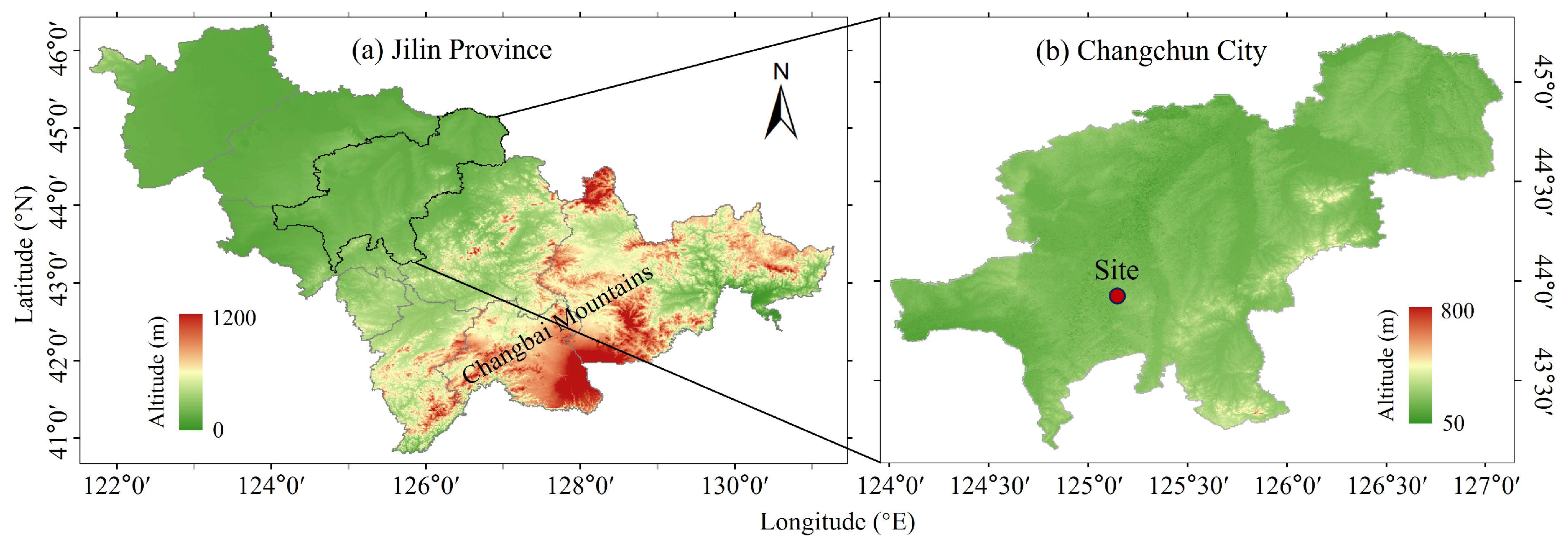
Changchun City (44°N, 125.5°E) is located in Jilin Province in the northeastern region of China and has a temperate continental semi-humid monsoon climate. Situated in the hinterland of the Northeast Plain, it lies in the hilly area of the Changbai Mountains to the southeast (see Figure 1). Due to low temperatures and dry weather in winter (Changchun’s temperature characteristics are winter-like climatic conditions in October–November), frequent cold air activities, and the generally flat terrain of Changchun with no significant surrounding mountain ranges to the southeast, which can block the winter monsoons from the north, the topography restricts air convection and diffusion, favoring the accumulation and retention of pollutants [21,22]. Additionally, as an important industrial city, Changchun has a relatively high level of pollutant emissions, especially during the winter heating season when atmospheric pollution is particularly severe [23,24,25]. The unique climatic and geographical conditions of Changchun, combined with industrial pollution and winter heating, result in a serious and complex haze problem [26,27]. In-depth research on the vertical distribution of water vapor during haze events in Changchun can contribute to a better understanding of the mechanisms behind haze formation.

Figure 1.
The topographic maps of (a) Jilin Province and (b) Changchun City.
In recent years, both domestic and international scholars have conducted extensive research on the haze formation process in Changchun and the North China region. Some studies have indicated that haze in Changchun is primarily influenced by a combination of meteorological conditions, topography, and emissions from pollution sources [23,28]. For example, under high humidity and low wind speed conditions, pollutants tend to accumulate, leading to severe haze phenomena [29]. Additionally, significant increases in PM2.5 concentrations due to coal combustion emissions during the winter heating season have been identified as a contributing factor to haze formation [24,25]. These studies have revealed various influencing factors of haze, but the specific role of water vapor in haze events has not been thoroughly explored. For instance, whether water vapor content exhibits vertical distribution characteristics similar to particulate matter during haze events and whether water vapor regulates the concentration of particulate matter remain unanswered questions.
Compared to traditional radiosondes, lidar technology, with its high temporal resolution, is capable of real-time monitoring of the vertical distribution of particulate matter and water vapor in the air, providing detailed information on the micro-dynamics of haze formation [30,31]. This enables us to gain a deeper understanding of the influence of water vapor at different altitudes on the formation and evolution of haze [32]. This study aims to deploy a three-wavelength Raman lidar system in Changchun to investigate the vertical distribution of atmospheric water vapor and aerosol optical parameters. Observational data from the autumn and winter seasons will be used for statistical analysis to reveal the characteristics of water vapor distribution in Northeast China during this period. Additionally, a specific haze event will be selected as a case study to analyze the role of water vapor in the formation and evolution of haze. Through these analyses, we aim to provide scientific insights into the dynamics of water vapor and haze during this particular event.
2. Instruments and Methods
2.1. Three-Wavelength Raman Lidar
Observations from a three-wavelength Raman lidar system were used in this study to illustrate spatiotemporal evolutions of aerosols and water vapor. This lidar system was deployed by the Meteorological Observation Center of China Meteorological Administration in the Green Park District (43.9°N, 125.22°E) of Changchun City. The system utilizes an Nd:YAG laser as the light source. The laser emits laser pulses at 355, 532, and 1064 nm, with a repetition frequency of 1 kHz and a pulse width of 2 ns. Signals collected by a 300 mm Cassegrain telescope are guided into the optical analyzing unit. Multiple sets of filters are employed in the optical analyzing unit to divide the returned signals into 8 channels. Channels 1 to 4 are used to receive parallel and perpendicular polarized signals at elastic wavelengths of 355 nm and 532 nm. Channels 5–7 are dedicated to detecting vibration Raman signals of nitrogen and water vapor molecules at wavelengths of 386, 407, and 607 nm, respectively. Channel 8 is used for the detection of a 1064 nm elastic signal. The raw data have a height resolution of 30 m and a time resolution of 1 min. Photon counting techniques are employed for signal detection at all channels. The main specifications of the lidar system are summarized in Table 1.

Table 1.
The main technical parameters of the three-wavelength Raman lidar system.
2.2. The Radiosonde
The radiosonde is another important atmospheric profiling tool used to obtain key parameters such as temperature, humidity, and air pressure on vertical profiles of the atmosphere [33,34]. By conducting regular radiosonde observations, we can gain insights into the vertical distribution of the meteorological parameters that may affect haze formation [34,35]. This study employs a domestically mainstream GNSS radiosonde, characterized by its small size, light weight, and long operational duration. The radiosonde conducts measurements twice daily, at 8:00 China Standard Time (CST, GMT+8) in the morning and 20:00 CST in the evening. The radiosonde station and the Raman lidar station are at the same location, with a maximum distance of no more than 30 m.
2.3. Water Vapor Retrieval Method and Calibration
The WVMR is an essential meteorological parameter describing water vapor and is one of the most important meteorological parameters [36]. It represents the physical quantity of air moisture and is defined as the ratio of the mass of water vapor to the mass of dry air within the same volume at a certain height . It is expressed as:
where represents the number density of water vapor molecules at height, represents the number density of dry air molecules; and represent the molecular weights of water vapor and dry air, respectively. Since nitrogen is an inert gas, its number density varies little over time and location and is relatively stable. In the troposphere, the ratio of nitrogen molecule number density to dry air molecule number density is almost constant (approximately 78%) [37]. The molecular weight of water vapor is 18.0 g/mol, and the molecular weight of dry air is 28.9 g/mol. Therefore, the number density of nitrogen molecules can be used instead of the number density of dry air for calculating the specific humidity, expressed as:
According to lidar equation [38], the power of the Raman scattering echo signals from atmospheric water vapor molecules and nitrogen molecules can be expressed as follows:
where the subscripts and represent water vapor molecules and nitrogen molecules, respectively, is the Raman channel factor, is the vibrational Raman backscatter cross-section of the molecules, is the molecular number density varying with height, , , and are the atmospheric transmittances at the laser wavelength , water vapor Raman scattering wavelength , and nitrogen Raman scattering wavelength , respectively. Their specific expressions are as follows:
where is the atmospheric extinction coefficient, the inversion formula for atmospheric specific humidity is represented as:
Here, we define the system calibration constant and the atmospheric transmittance correction function as follows:
Therefore, the WVMR can be expressed as:
According to Equation (8), if the system calibration constant and the atmospheric transmittance correction function are known, using the ratio of the Raman scattering echo signals from water vapor and nitrogen molecules detected by the Raman lidar system, the height distribution of the WVMR can be retrieved.
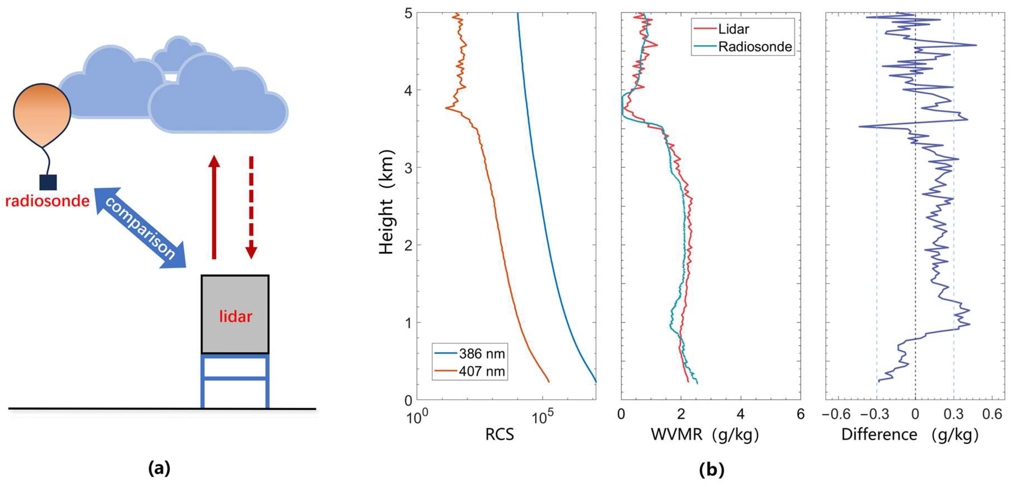
As the measurement results of the lidar are influenced by system parameters, calibration of the lidar measurement results is necessary to obtain the WVMR [39,40]. A schematic diagram of the calibration experiment is shown in Figure 2a, where the water vapor Raman channel is typically calibrated using a radiosonde [41,42]. To ensure high accuracy, lidar calibration is generally performed under stable atmospheric conditions [40]. After meeting the atmospheric conditions, an appropriate height range is selected to calibrate the WVMR measured by the lidar, resulting in the determination of calibration constants. The expression for the calibration constant is as follows:
where is the WVMR obtained from the radiosonde, is the number of points corresponding to the calibration range, and are the echo light signals of the water vapor channel and the nitrogen channel, respectively, and is the atmospheric transmittance from height to height . Figure 2b illustrates an example of atmospheric water vapor layer inversion and calibration conducted under clear weather conditions.
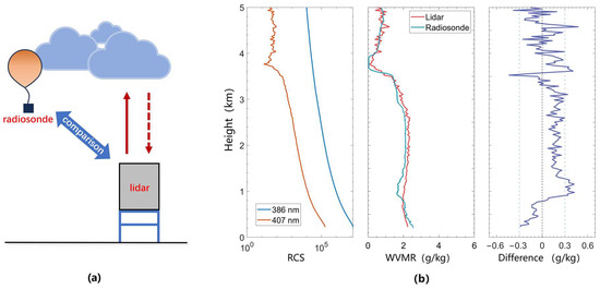
Figure 2.
(a) Schematic diagram of water vapor calibration experiment; (b) from left to right are the range corrected signal (RCS), WVMR, and the absolute deviation between the lidar and the radiosonde (with ±0.3 g/kg line marked), measured at 20:00 CST on 18 October 2023.
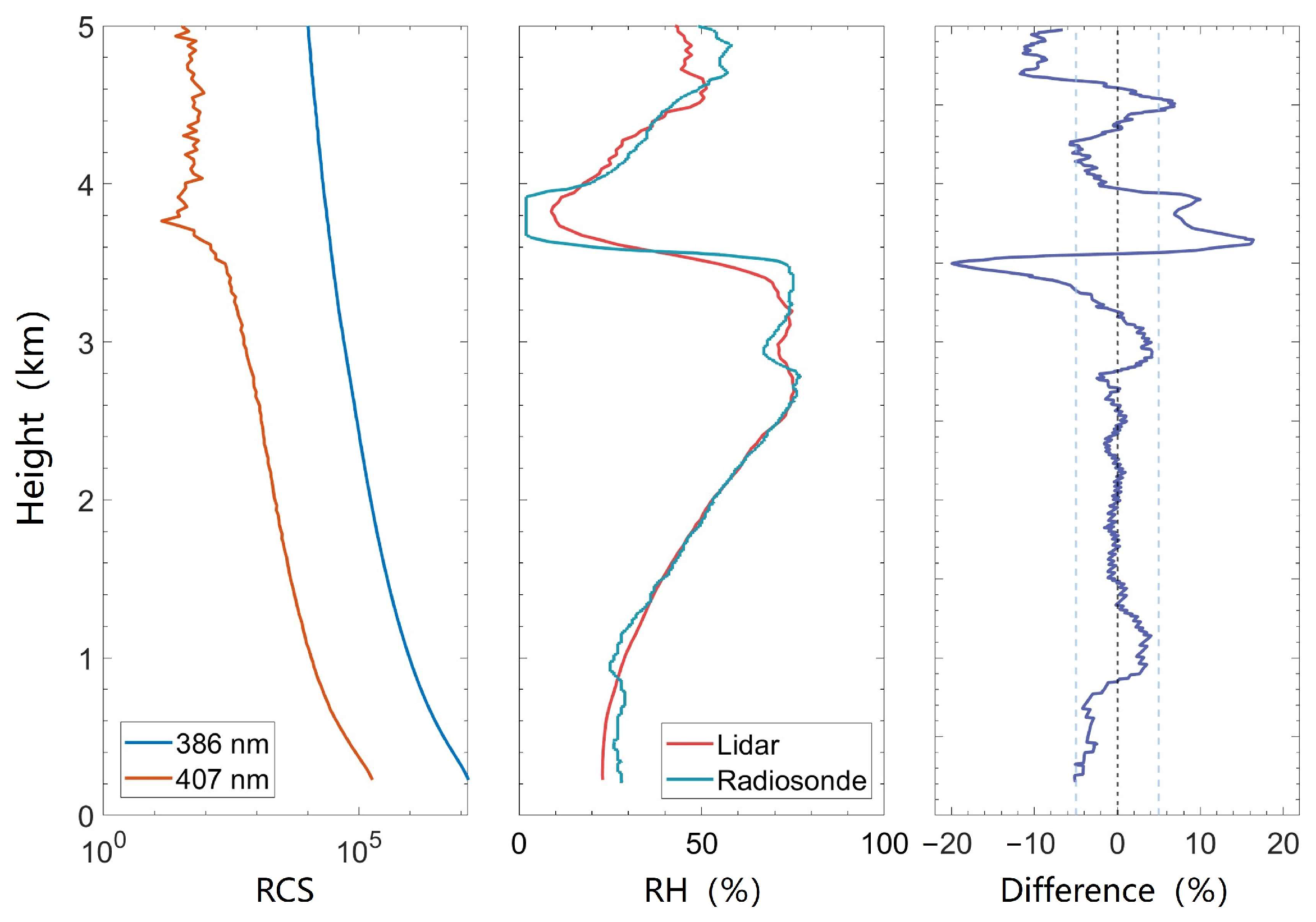
Relative humidity (RH) is a physical quantity that indicates the dryness or wetness of the air [43,44], and the transformation processes between fog and haze in the atmosphere are closely related to the level of RH [45,46,47]. RH is defined as the percentage of the actual water vapor density in a unit volume of air to the saturated water vapor density at the same temperature [44,48]. It is represented as :
In the equation, represents the number density of water vapor molecules at a certain height , and is the saturated water vapor density at height , which is a function of temperature. The relationship between the saturated water vapor density and the atmospheric temperature (in degrees Celsius) is given by the following formula:
where is the saturated water vapor pressure at that temperature in . This can be calculated (see Equation (12)) using the Tetens empirical formula [49]. Figure 3 shows the results of the RH inversion performed under clear weather conditions.
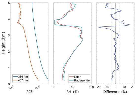
Figure 3.
From left to right are the RCS, RH, and the deviation of RH between the lidar and the radiosonde (with a ±5% line marked), measured at 20:00 CST on 18 October 2023.
2.4. Retrievals of Aerosol Optical Properties from Lidar
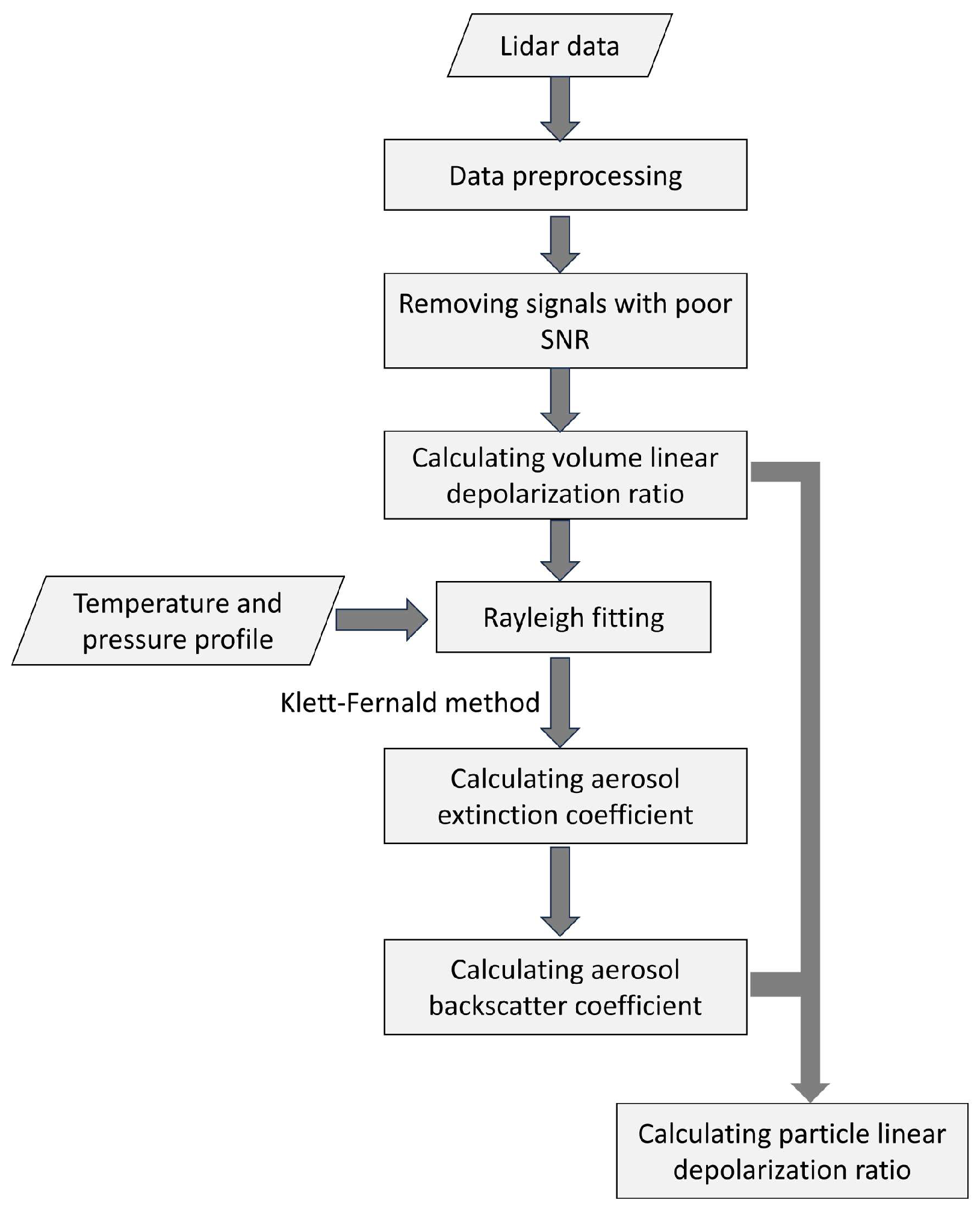
This paper analyzes the distribution and characteristics of aerosols in the atmosphere through the retrieval of aerosol optical properties. The optical retrieval process mainly involves the calculation of the extinction coefficient, backscatter coefficient, and particle depolarization ratio, with the overall computational workflow illustrated in Figure 4. First, raw data are acquired from the lidar and undergo preprocessing, including trigger delay correction, dead-time correction, and overlap correction [50,51]. Next, the signal-to-noise ratio (SNR) is calculated, and signals with poor SNR are removed to ensure data accuracy and validity [52]. Using temperature and pressure profile data derived from the standard atmosphere model [53], rayleigh fitting is performed [52]. Subsequently, the extinction and backscatter coefficients of aerosols are calculated using the Klett–Fernald method [54,55,56]. Finally, the particle depolarization ratio is calculated based on these results.
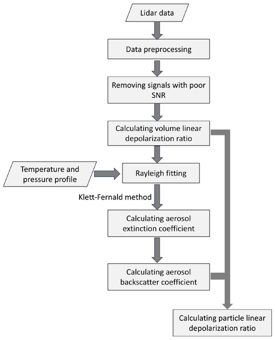
Figure 4.
Flowchart for aerosol optical parameter retrieval.
3. Analysis
3.1. The Distribution Characteristics and Variations of Water Vapor Vertical Profiles
Water vapor profiles for Changchun city during the evenings of October 2023 (CST 19:00–21:00) were collected using the three-wavelength Raman lidar system due to the low background noise of water vapor Raman channel during nighttime and for the consideration of inter-comparison with radiosonde measurements launching at 20:00 CST. Analysis of these data yielded vertical profiles of water vapor, which were used to analyze the distribution characteristics and variations of water vapor in Changchun City. Measurements were not conducted on certain dates (2nd, 3rd, 4th, 6th, 13th, and 14th) of October due to maintenance and system updates of the lidar system.
Water vapor is a rapidly changing component of the atmosphere, with its distribution varying widely across different regions [57]. Since water vapor above 10 km is relatively scarce [58], this study primarily focuses on the distribution characteristics of water vapor below 10 km. Precipitable water vapor (PWV) can, to some extent, reflect the current atmospheric water vapor content [59,60]. Based on these data (excluding the near-surface signal blind zone of the lidar), we conducted a statistical analysis of the PWV at heights of 0.25–5 km and 0.25–10 km, and calculated the proportion of PWV at 0.25–5 km height relative to the overall content.
Figure 5 depicts the variations in nighttime mean PWV at heights of 0.25–5 km and 0.25–10 km, along with the corresponding proportions. In Changchun, the proportion of PWV between 0.25 and 5 km relative to 0.25–10 km ranges from 64% to 99%, with an average proportion of 88.3%. This result reflects the vertical distribution characteristics of water vapor content in the Changchun area, indicating that atmospheric water vapor content is primarily concentrated below 5 km, accounting for 64% to 99% of the total water vapor content below 10 km.
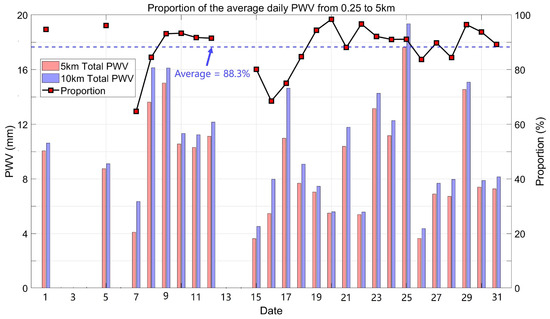
Figure 5.
The proportion of daily PWV at 0.25–5 km in October.
In terms of vertical variation of water vapor, the atmospheric WVMR varies significantly with altitude and exhibits distinct stratification. The figure displays the distribution of WVMR variations during representative nights in October. To analyze the sharp changes in WVMR, logarithmic coordinates are used for representation.
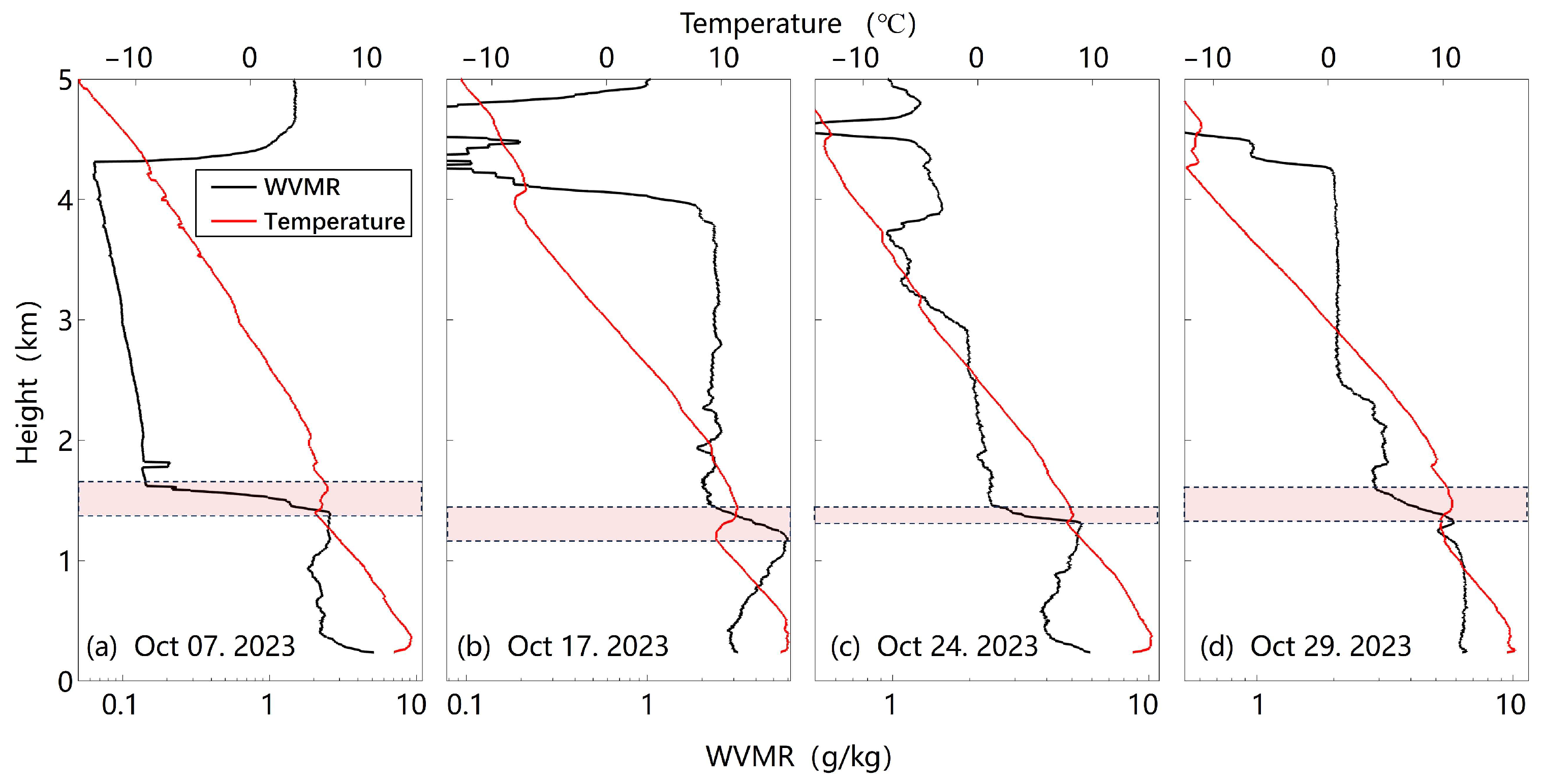
As shown in Figure 6a, the WVMR profile obtained at 20:00 on 7 October 2023, under cloudy conditions, exhibits a significant decrease from 5 g/kg to 0.1 g/kg below 4.3 km, while above 4.3 km, the water vapor content increases due to the presence of clouds. It is noteworthy that a sudden decrease in water vapor content can be observed within the range of 1.2 km to 1.6 km. The WVMR drops from approximately 1 g/kg to around 0.1 g/kg, a phenomenon referred to as an abrupt change in the water vapor profile [61,62]. Figure 6b–d show other representative measurement results, indicating abrupt changes in water vapor content within the height ranges of 1.1 km to 1.5 km, 1.4 km to 1.6 km, and 1.4 km to 1.7 km, respectively. According to the temperature profile from radiosonde measurements, such discontinuities are accompanied by the appearance of inversions. The data from these nocturnal observations suggest that there was a noticeable variation in water vapor content between 1 km and 3 km. This result indicates that a higher concentration of water vapor was present below 3 km, which may be associated with the formation of haze weather.
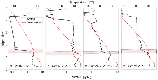
Figure 6.
Representative measurement instances of WVMR during the nighttime of October 2023. The red-shaded areas within the dashed boxes indicate the height ranges where abrupt changes in water vapor. The weather conditions from left to right are (a) cloudy, (b) sunny, (c) light haze, and (d) moderate haze.
3.2. The Variation of Water Vapor during Haze Events
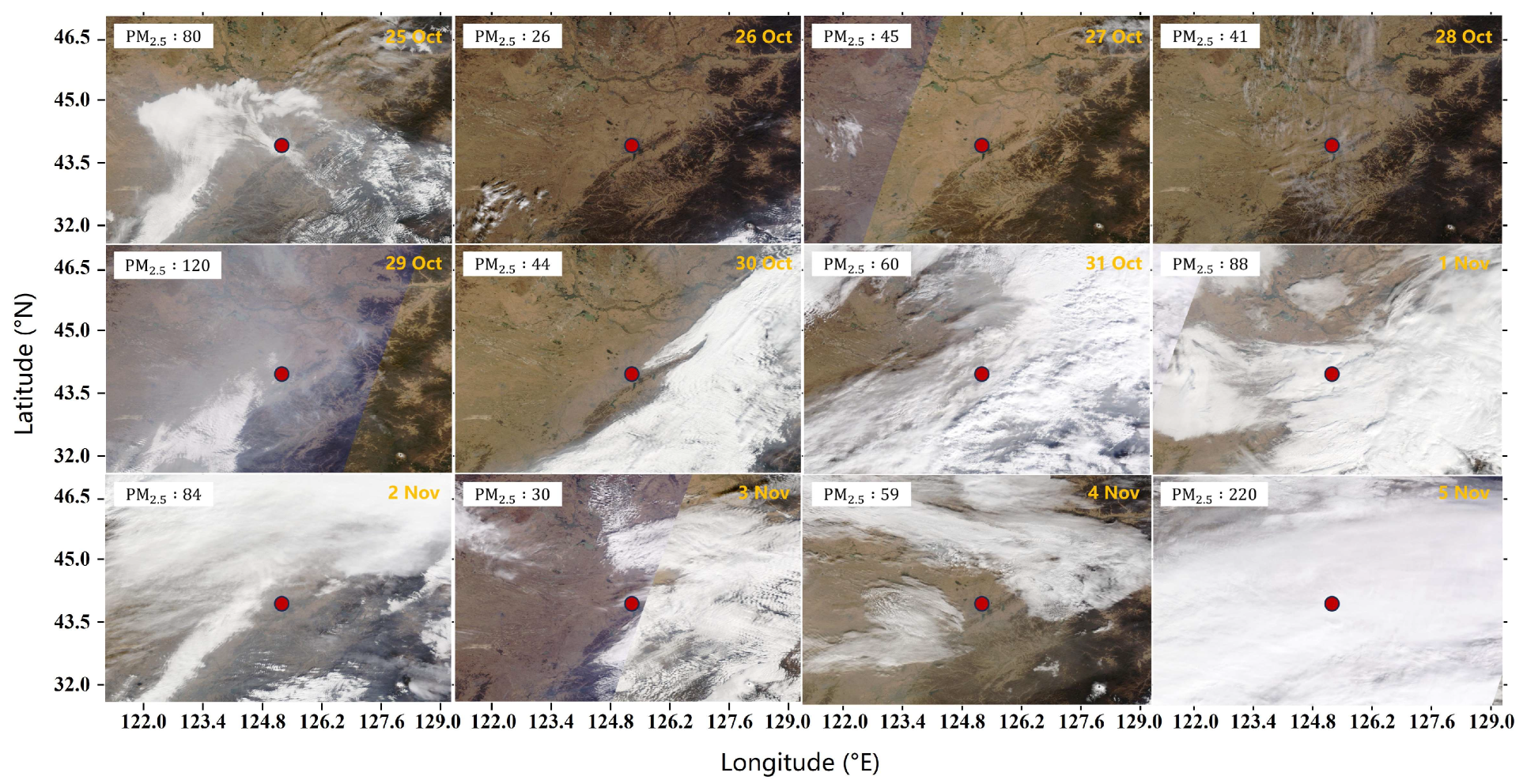
We analyzed persisting haze events in Changchun from 25 October 2023 to 5 November 2023. During this period, satellite true-color images (Figure 7) and wind field maps (Figure 8) show that moderate haze occurred on 29 October, with PM2.5 concentrations reaching 120 μg/m3, gradually dissipating by 30 October. The haze intensified again on 31 October due to a change in wind direction, persisting until 2 November. On 4 November, there was a recurrence of light haze, which transitioned into severe haze on 5 November, with PM2.5 concentrations peaking at 220 μg/m3. The PM concentration data were measured at the same site using the filter membrane weighing method [63], with a time resolution of 1 h. Analysis of the wind field maps suggests that strong winds from the northeast may have transported a large amount of aerosols from distant areas to Changchun. However, due to the obstruction of the Changbai Mountains, pollutants accumulated in the northern part of the Changbai Mountains. This situation exacerbated haze formation in the Changchun area to some extent.

Figure 7.
MODIS Terra true-color images during the haze event period. The red dot is the measuring station. The top left corner of the images indicates the average PM2.5 (μg/m3) concentration for the day.
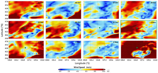
Figure 8.
Wind field maps (altitude of 100 m) during the haze event period. The green dot is the measuring station.
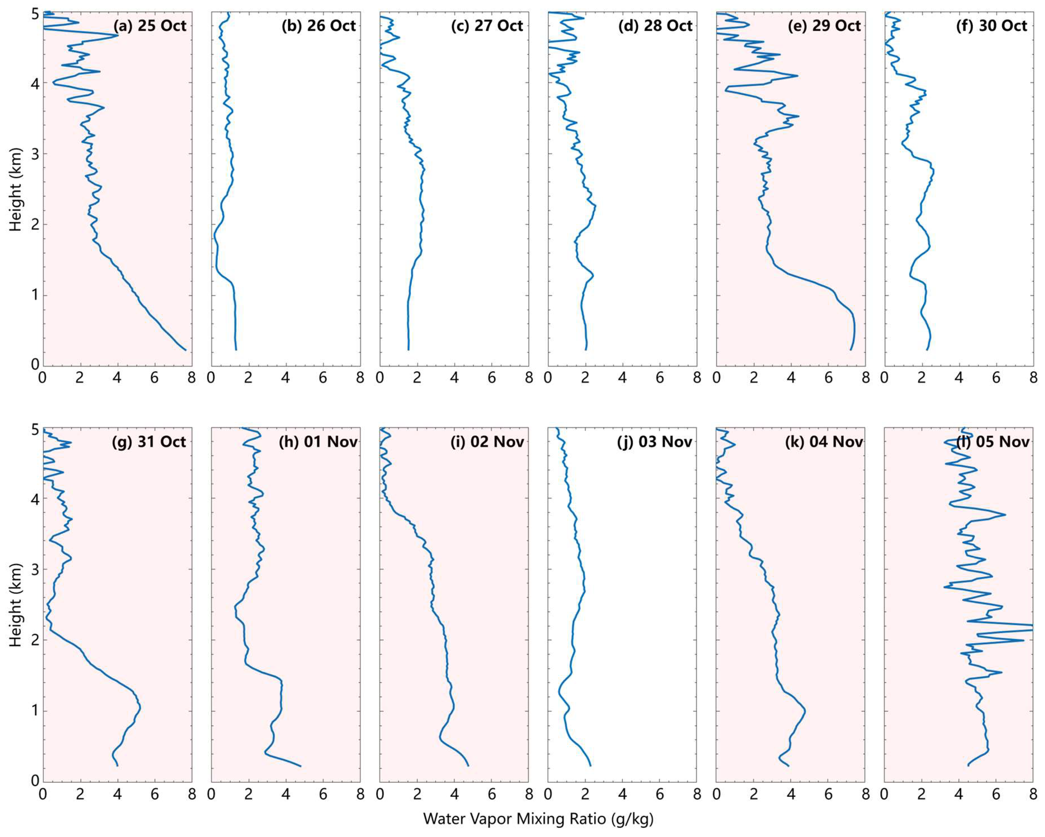
During this event, we focused on analyzing the variation of atmospheric water vapor. It can be observed that there were several transitions from hazy weather to clear conditions over the two-week observation period. Figure 9 presents consecutive WVMR profiles during the event. Here, we mainly discuss the variation of water vapor content below 3 km. Figure 9e shows the water vapor profile under haze conditions at 20:00 CST on 29 November, where significantly higher water vapor content, averaging 6 g/kg, is observed within 1 km, gradually decreasing with height. In the altitude range of 2 km to 3 km, the average WVMR is 2 g/kg. Figure 9f presents the water vapor profile under clear weather conditions, exhibiting a more uniform vertical distribution of water vapor content with an average WVMR of 2 g/kg within 3 km. Similar trends in water vapor profiles were observed at other times during this event. It is evident that there are significant differences in the vertical distribution of water vapor content between hazy and clear weather conditions.

Figure 9.
WVMR profiles from 25 October to 5 November 2023, obtained by lidar, averaged between 19:00 and 21:00 CST on each day. The red shading indicates the days when haze weather occurred.
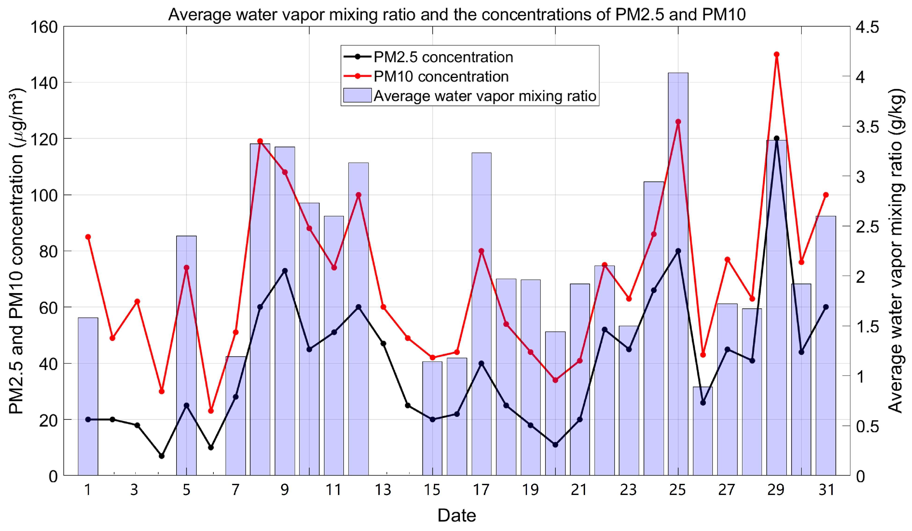
To further analyze the water vapor characteristics under haze conditions, the average WVMR below 3 km in October was analyzed, as shown in Figure 10. The daily average WVMR in October varied greatly, with a maximum value of 4 g/kg and a minimum value of 0.8 g/kg. The daily average WVMR was relatively high on the 8th, 9th, 17th, 25th, and 29th, ranging from 3.3 to 4 g/kg. On the 7th, 15th, 16th, and 26th, the daily average WVMR was relatively low, ranging from 0.8 to 1.2 g/kg. Considering the occurrence of haze weather on the 25th, followed by clear weather until the 28th, and then moderate haze weather on the 29th, it can be seen that the atmospheric average water vapor content is lower during clear weather and higher during haze weather. During haze formation, the average WVMR below 3 km is three to four times higher than that in clear weather.
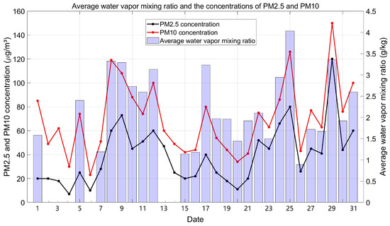
Figure 10.
The daily average WVMR and the concentrations of PM2.5 and PM10 for October 2023.
The concentration curves of PM2.5 and PM10 are also provided in Figure 10, showing variations corresponding to changes in weather conditions. During the haze weather on 29 October, when the average WVMR was relatively high (4 g/kg), the concentrations of PM2.5 and PM10 were also high, at 120 μg/m3 and 150 μg/m3, respectively. However, under clear weather on the 30th, the concentrations of PM2.5 and PM10 significantly decreased to 44 μg/m3 and 76 μg/m3, respectively. It can be observed that the variations in PM2.5 and PM10 concentrations are highly consistent with the changes in WVMR.
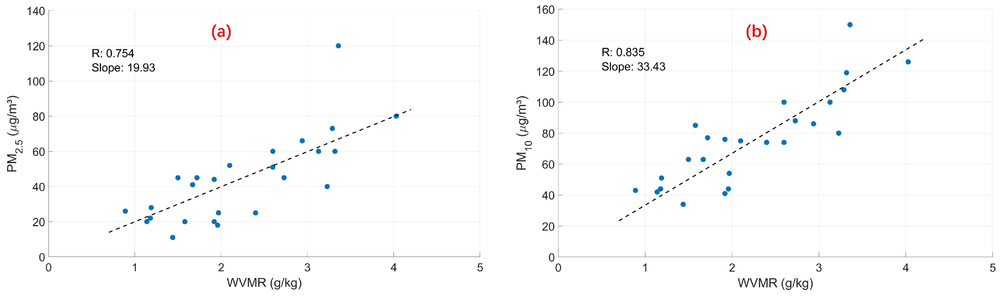
We analyzed the correlation between the average (0–3 km) WVMR and the concentrations of PM2.5 and PM10, as shown in Figure 11. We found that the average WVMR has a strong positive correlation with the concentrations of PM2.5 and PM10 (correlation coefficient of 0.754 for PM2.5 and 0.835 for PM10).
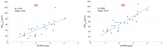
Figure 11.
The correlation between the daily average (0–3 km) WVMR and the concentrations of PM2.5 (a) and PM10 (b) in October 2023.
It is evident that during the autumn and winter seasons, when water vapor content is relatively low, there is a positive correlation between water vapor content and the PM index in the Changchun area. To some extent, the haze can be represented by the concentration of particulate matter [64,65,66]. Therefore, we infer that the increase in water vapor content below the boundary layer has a significant impact on haze formation and that the formation of haze is closely related to changes in water vapor content. Consequently, water vapor data can be used to a certain extent for the monitoring and forecasting of haze weather.
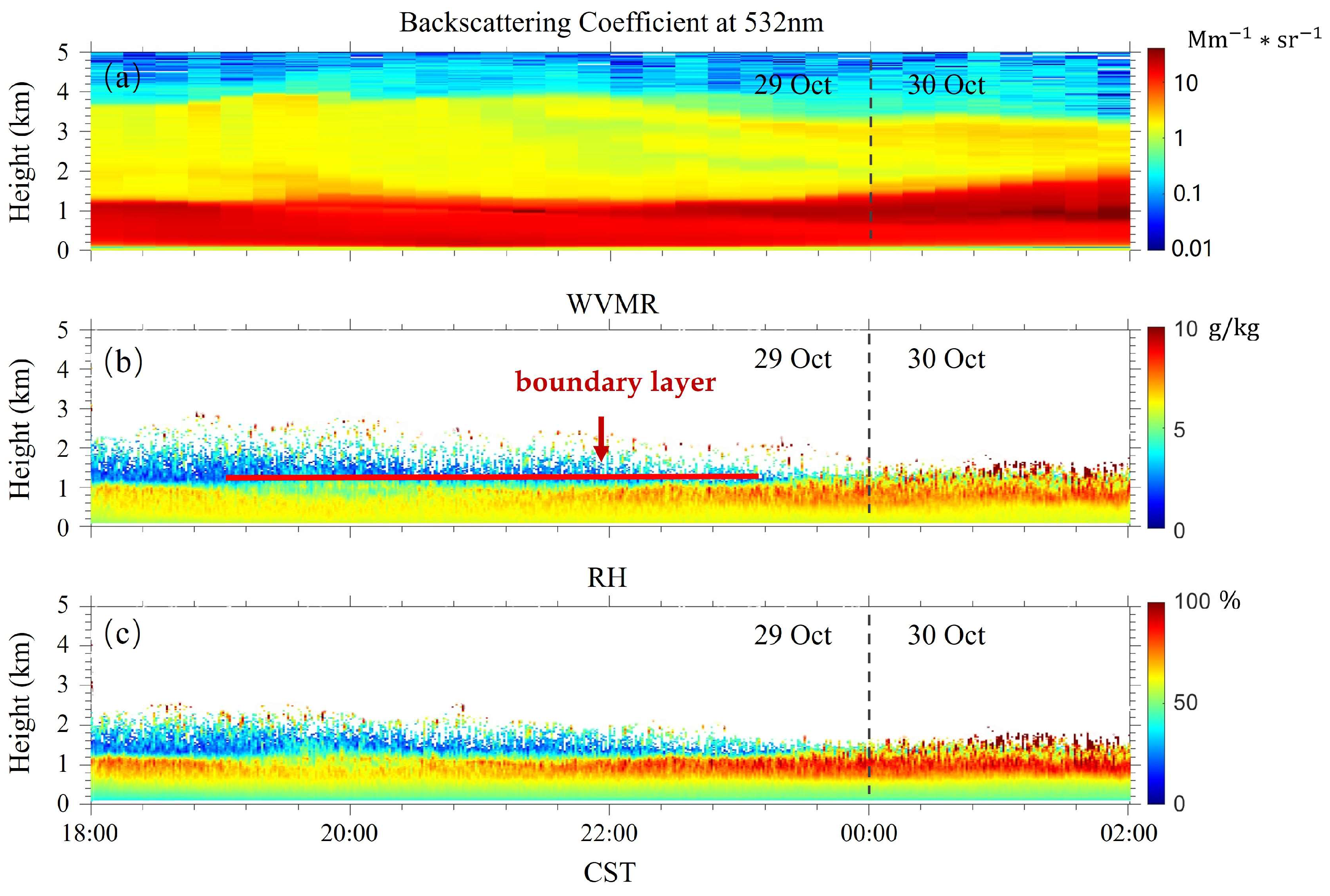
To further analyze the impact of aerosols on haze formation, a typical haze event during the period was selected for aerosol and water vapor analysis. Figure 12 shows the variations in aerosol backscattering coefficients, WVMR, and RH with height in the atmosphere over Changchun from 18:00 CST on 29 October to 02:00 CST on 30 October 2023. The atmospheric boundary layer [67,68], determined using the potential temperature gradient method [69,70], has a height of approximately 1.2 km. It can be observed that the backscattering coefficient within the boundary layer is significantly higher, indicating a notable accumulation of aerosols in this layer. With increasing height, the aerosol concentration decreases significantly. Over time, the aerosol content within the boundary layer gradually increases and spreads upward to 2 km. Simultaneously, the WVMR values within the boundary layer are primarily around 6 g/kg and gradually increase to 7 g/kg over time, with a relatively uniform distribution. Above the boundary layer, atmospheric water vapor content decreases gradually, RH also declines, and aerosol content correspondingly decreases. It is evident that there is a significant correlation between water vapor content and aerosol concentration below the boundary layer.

Figure 12.
(a) Aerosol backscattering coefficient, (b) WVMR, and (c) RH continuously detected by lidar from 18:00 CST on October 29 to 02:00 CST on 30 October 2023.
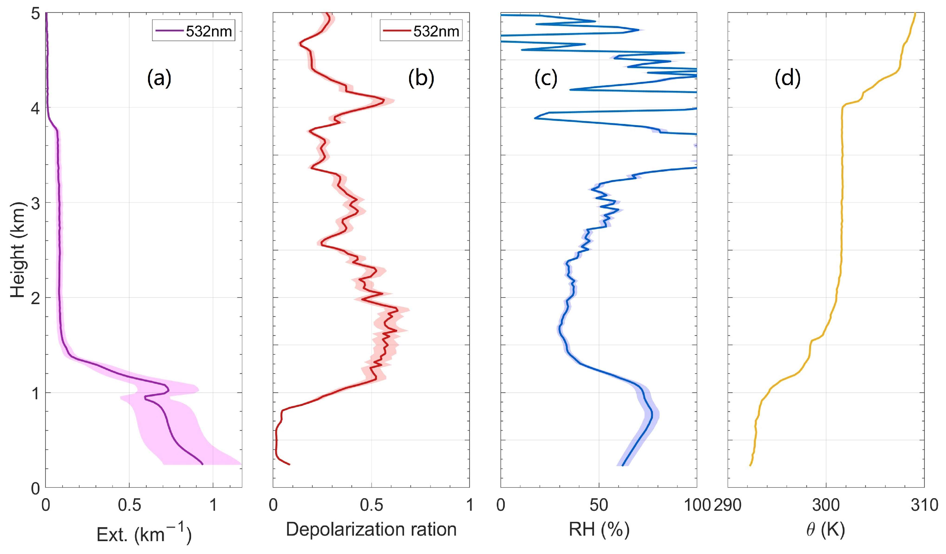
Figure 13 shows the vertical profiles of the extinction coefficient, depolarization ratio, RH, and potential temperature at 20:00 CST on the same day. It can be seen that the water vapor content within the boundary layer still shows a good positive correlation with the particle concentration, which may be due to the influence of water vapor on aerosols. Figure 13a,c indicate that below the boundary layer, the aerosol content and RH remain stable and exhibit a linear decreasing trend over a wide range. This likely suggests that nighttime water vapor content promotes the hygroscopic growth of aerosols, resulting in good mixing between water vapor and particles. Figure 13b shows that, in this case, the particle depolarization ratio remains low and exhibits a linear increasing trend at this height, indicating that the particles are primarily spherical [71,72]. In environments with high water vapor content, aerosol particles adsorb a significant amount of water vapor on their surfaces, increasing their hygroscopicity. These wet, spherical aerosol particles have enhanced abilities to absorb and scatter light. Additionally, the presence of water vapor alters the refractive index of the atmospheric medium, which further affects atmospheric visibility and contributes to haze formation.

Figure 13.
Vertical profiles at 20:00 CST on 29 October 2023. From left to right, (a) extinction coefficients, (b) particle depolarization ratio, (c) RH, and (d) potential temperature, in which the shaded area denotes the uncertainty. Products at the lowest heights from the surface to 500 m are filtered out due to the incomplete overlap factor of the lidar system.
Through a detailed analysis of the spatiotemporal height profiles and vertical profiles of aerosols and water vapor during a typical haze event, we observed that when the WVMR stabilizes within a certain range, the atmospheric boundary layer also gradually remains relatively stable. This results in a significant limitation on the vertical transport and diffusion of aerosols. In this environment, aerosol content within the boundary layer increases with rising water vapor content, and water vapor also promotes the hygroscopic growth of aerosols, making the aerosol particles more spherical. Specifically, within the boundary layer, high water vapor content stabilizes the inversion layer, hindering the vertical upward diffusion of aerosol particles. Analysis of aerosol optical properties and vertical water vapor profiles reveals that high water vapor content likely promotes the hygroscopic growth of aerosol particles, further increasing their size and mass, which leads to an increase in the aerosol extinction coefficient. This process results in a higher concentration of particulate matter in the atmosphere and reduced visibility, exacerbating the severity of haze.
4. Conclusions
This study utilized a three-wavelength Raman lidar system to retrieve atmospheric WVMR and verified its feasibility. Data of atmospheric WVMR profiles were collected, and observational data from 19:00 to 21:00 (CST) from October to November 2023 in the Changchun region were selected for the analysis of vertical distribution characteristics and variations of atmospheric water vapor.
Through horizontal observations using satellite true-color images and wind field maps, we analyzed the severe haze event in the Changchun region between 25 October and 5 November. Vertical observations using a multi-wavelength Raman lidar system were then conducted to focus on the variations in atmospheric water vapor content. We found that under haze conditions, water vapor content was significantly higher at lower altitudes and gradually decreased with increasing altitude. In contrast, under clear weather conditions, water vapor content was lower and more uniformly distributed with altitude. Further analysis of the water vapor characteristics during haze weather conditions involved analyzing the vertically-averaged WVMR below 3 km for October. We observed that under clear weather conditions, the atmospheric average water vapor content was lower, whereas under haze conditions, it was higher. During haze formation, the average WVMR within 3 km altitude was three to four times higher than that during clear weather. Additionally, the variations in PM2.5 and PM10 concentrations showed a positive correlation with the changes in average WVMR, with the PM2.5 correlation coefficient greater than 0.7 and the PM10 correlation coefficient greater than 0.8. These results suggest that the increase in water vapor content in the boundary layer during this event may have contributed to the formation of haze, highlighting a close relationship between the haze event and fluctuations in water vapor content. A thorough analysis of the spatiotemporal height profiles and vertical profiles of aerosols and water vapor during a typical haze event revealed several key insights. We observed that below the boundary layer, the distribution of WVMR was uniform. As the altitude increased beyond the boundary layer, atmospheric water vapor content gradually decreased, accompanied by a decrease in RH. Furthermore, a strong positive correlation was observed between the aerosol extinction coefficient and backscatter coefficient below the boundary layer and the WVMR, especially during haze events. This positive correlation might stem from the influence of water vapor on aerosols.
Through the spatiotemporal height profiles and in-depth analysis of the backscattering coefficients and water vapor during a typical haze event, we found that within the boundary layer, there is a high positive correlation between aerosol concentration and the WVMR. This positive correlation is likely due to the influence of water vapor on aerosols. To analyze this effect, we examined vertical profiles of various parameters at 20:00 CST during a haze event. We observed that the relative stability of the atmospheric boundary layer may hinder the vertical transport and diffusion of aerosols and lead to the accumulation of water vapor. High water vapor content stabilizes the inversion layer, which, in turn, makes the atmospheric boundary layer even more stable. The analysis revealed that high water vapor content could be a factor influencing the hygroscopic growth of aerosol particles, potentially making them more spherical. The presence of water vapor might also have affected the optical properties of aerosols, leading to stronger signal responses in lidar observations and a sharp increase in the aerosol extinction coefficient. This process results in higher particulate matter concentrations and reduced visibility, exacerbating the severity of haze. These observations emphasize the critical role of water vapor in haze formation and evolution and highlight the impact of the interactions between water vapor and aerosols on haze events.
Author Contributions
Conceptualization, T.Z. and Z.Y.; methodology, Z.Y.; software, Y.W.; validation, T.Z., Z.Y. and Y.W.; formal analysis, T.Z.; investigation, T.Z. and Y.Z.; resources, Y.D. and X.D.; data curation, T.Z.; writing—original draft preparation, T.Z.; writing—review and editing, T.Z., L.W. (Longlong Wang), Y.G., L.W. (Lude Wei), Q.Z. and D.H.; visualization, T.Z. and Y.W; supervision, Y.Z.; project administration, T.Z.; funding acquisition, Y.Z. All authors have read and agreed to the published version of the manuscript.
Funding
This research was funded by the National Key Research and Development Program of China (2023YFC3007802) and the National Natural Science Foundation of China (NSFC) (42205130, 62105248 and 62475068).
Data Availability Statement
The datasets generated during and/or analyzed during the current study are available from the corresponding author on reasonable request.
Acknowledgments
The authors would like to thank NASA and ECMWF for providing the Terra satellite data and the wind field data, respectively. They would also like to thank the Meteorological Observation Centre, China Meteorological Administration, for providing Lidar data.
Conflicts of Interest
Author Tianpei Zhang was employed by the company Wuhan Yike Photonics Co., Ltd. The remaining authors declare that the research was conducted in the absence of any commercial or financial relationships that could be construed as a potential conflict of interest.
References
- Bevis, M.; Businger, S.; Herring, T.A.; Rocken, C.; Anthes, R.A.; Ware, R.H. GPS meteorology: Remote sensing of atmospheric water vapor using the global positioning system. J. Geophys. Res. Atmos. 2012, 97, 15787–15801. [Google Scholar] [CrossRef]
- Rocken, C.; Ware, R.; Van Hove, T.; Solheim, F.; Alber, C.; Johnson, J.; Bevis, M.; Businger, S. Sensing atmospheric water vapor with the global positioning system. Geophys. Res. Lett. 2012, 20, 2631–2634. [Google Scholar] [CrossRef]
- Trenberth, K.E.; Fasullo, J.; Smith, L. Trends and variability in column-integrated atmospheric water vapor. Clim. Dyn. 2005, 24, 741–758. [Google Scholar] [CrossRef]
- King, M.D.; Menzel, W.P.; Kaufman, Y.J.; Tanre, D.; Bo-Cai, G.; Platnick, S.; Ackerman, S.A.; Remer, L.A.; Pincus, R.; Hubanks, P.A. Cloud and aerosol properties, precipitable water, and profiles of temperature and water vapor from MODIS. IEEE Trans. Geosci. Remote Sens. 2003, 41, 442–458. [Google Scholar] [CrossRef]
- Bengtsson, L. The global atmospheric water cycle. Environ. Res. Lett. 2010, 5, 025202. [Google Scholar] [CrossRef]
- Held, I.M.; Soden, B.J. Water Vapor Feedback and Global Warming. Annu. Rev. Energy Environ. 2000, 25, 441–475. [Google Scholar] [CrossRef]
- Hao, J.; Lu, E. Variation of Relative Humidity as Seen through Linking Water Vapor to Air Temperature: An Assessment of Interannual Variations in the Near-Surface Atmosphere. Atmosphere 2022, 13, 1171. [Google Scholar] [CrossRef]
- Ramadan, Z.; Song, X.H.; Hopke, P.K. Identification of sources of Phoenix aerosol by positive matrix factorization. J. Air Waste Manag. Assoc. 2000, 50, 1308–1320. [Google Scholar] [CrossRef] [PubMed]
- Gao, J.; Woodward, A.; Vardoulakis, S.; Kovats, S.; Wilkinson, P.; Li, L.; Xu, L.; Li, J.; Yang, J.; Li, J.; et al. Haze, public health and mitigation measures in China: A review of the current evidence for further policy response. Sci. Total Environ. 2017, 578, 148–157. [Google Scholar] [CrossRef]
- Pérez-Díaz, J.; Ivanov, O.; Peshev, Z.; Álvarez-Valenzuela, M.; Valiente-Blanco, I.; Evgenieva, T.; Dreischuh, T.; Gueorguiev, O.; Todorov, P.; Vaseashta, A. Fogs: Physical Basis, Characteristic Properties, and Impacts on the Environment and Human Health. Water 2017, 9, 807. [Google Scholar] [CrossRef]
- Guo, L.; Guo, X.; Fang, C.; Zhu, S. Observation analysis on characteristics of formation, evolution and transition of a long-lasting severe fog and haze episode in North China. Sci. China Earth Sci. 2014, 58, 329–344. [Google Scholar] [CrossRef]
- Lakra, K.; Avishek, K. A review on factors influencing fog formation, classification, forecasting, detection and impacts. Rend. Lincei. Sci. Fis. Nat. 2022, 33, 319–353. [Google Scholar] [CrossRef] [PubMed]
- Willett, H.C. Fog and haze, their causes, distribution, and forecasting. Mon. Weather. Rev. 1928, 56, 435–468. [Google Scholar] [CrossRef]
- Yu, C.; Zhao, T.; Bai, Y.; Zhang, L.; Kong, S.; Yu, X.; He, J.; Cui, C.; Yang, J.; You, Y.; et al. Heavy air pollution with a unique “non-stagnant” atmospheric boundary layer in the Yangtze River middle basin aggravated by regional transport of PM2.5 over China. Atmos. Chem. Phys. 2020, 20, 7217–7230. [Google Scholar] [CrossRef]
- Zhao, D.; Xin, J.; Gong, C.; Quan, J.; Liu, G.; Zhao, W.; Wang, Y.; Liu, Z.; Song, T. The formation mechanism of air pollution episodes in Beijing city: Insights into the measured feedback between aerosol radiative forcing and the atmospheric boundary layer stability. Sci. Total Environ. 2019, 692, 371–381. [Google Scholar] [CrossRef] [PubMed]
- Malap, N.; Prabha, T.V.; Karipot, A. Impact of middle atmospheric humidity on boundary layer turbulence and clouds. J. Atmos. Sol. Terr. Phys. 2021, 215, 105553. [Google Scholar] [CrossRef]
- Behrendt, A.; Nakamura, T.; Onishi, M.; Baumgart, R.; Tsuda, T. Combined Raman lidar for the measurement of atmospheric temperature, water vapor, particle extinction coefficient, and particle backscatter coefficient. Appl. Opt. 2002, 41, 7657–7666. [Google Scholar] [CrossRef]
- Barnes, J.E.; Kaplan, T.; Vömel, H.; Read, W.G. NASA/Aura/Microwave Limb Sounder water vapor validation at Mauna Loa Observatory by Raman lidar. J. Geophys. Res. Atmos. 2008, 113, D15S03. [Google Scholar] [CrossRef]
- Jia, J.; Yi, F. Atmospheric temperature measurements at altitudes of 5-30 km with a double-grating-based pure rotational Raman lidar. Appl. Opt. 2014, 53, 5330–5343. [Google Scholar] [CrossRef]
- Wang, Y.; Cao, X.; He, T.; Gao, F.; Hua, D.; Zhao, M. Observation and analysis of the temperature inversion layer by Raman lidar up to the lower stratosphere. Appl. Opt. 2015, 54, 10079–10088. [Google Scholar] [CrossRef]
- Steyn, D.G.; De Wekker, S.F.; Kossmann, M.; Martilli, A. Boundary layers and air quality in mountainous terrain. In Muntain Weather Research and Forecasting; Springer: Dordrecht, The Netherlands, 2013; pp. 261–289. [Google Scholar] [CrossRef]
- Giovannini, L.; Ferrero, E.; Karl, T.; Rotach, M.W.; Staquet, C.; Trini Castelli, S.; Zardi, D. Atmospheric Pollutant Dispersion over Complex Terrain: Challenges and Needs for Improving Air Quality Measurements and Modeling. Atmosphere 2020, 11, 646. [Google Scholar] [CrossRef]
- Ma, S.; Chen, W.; Zhang, S.; Tong, Q.; Bao, Q.; Gao, Z. Characteristics and cause analysis of heavy haze in Changchun City in Northeast China. Chin. Geogr. Sci. 2017, 27, 989–1002. [Google Scholar] [CrossRef]
- Zhao, H.; Ma, Y.; Wang, Y.; Wang, H.; Sheng, Z.; Gui, K.; Zheng, Y.; Zhang, X.; Che, H. Aerosol and gaseous pollutant characteristics during the heating season (winter–spring transition) in the Harbin-Changchun megalopolis, northeastern China. J. Atmos. Sol. Terr. Phys. 2019, 188, 26–43. [Google Scholar] [CrossRef]
- Li, B.; Shi, X.F.; Liu, Y.P.; Lu, L.; Wang, G.L.; Thapa, S.; Sun, X.Z.; Fu, D.L.; Wang, K.; Qi, H. Long-term characteristics of criteria air pollutants in megacities of Harbin-Changchun megalopolis, Northeast China: Spatiotemporal variations, source analysis, and meteorological effects. Environ. Pollut. 2020, 267, 115441. [Google Scholar] [CrossRef] [PubMed]
- Wang, S.; Li, Y.; Haque, M. Evidence on the Impact of Winter Heating Policy on Air Pollution and Its Dynamic Changes in North China. Sustainability 2019, 11, 2728. [Google Scholar] [CrossRef]
- Zhang, M.; Zhang, S.; Bao, Q.; Yang, C.; Qin, Y.; Fu, J.; Chen, W. Temporal Variation and Source Analysis of Carbonaceous Aerosol in Industrial Cities of Northeast China during the Spring Festival: The Case of Changchun. Atmosphere 2020, 11, 991. [Google Scholar] [CrossRef]
- Chen, W.; Zhang, S.; Tong, Q.; Zhang, X.; Zhao, H.; Ma, S.; Xiu, A.; He, Y. Regional Characteristics and Causes of Haze Events in Northeast China. Chin. Geogr. Sci. 2018, 28, 836–850. [Google Scholar] [CrossRef]
- Meng, C.; Cheng, T.; Bao, F.; Gu, X.; Wang, J.; Zuo, X.; Shi, S. The Impact of Meteorological Factors on Fine Particulate Pollution in Northeast China. Aerosol Air Qual. Res. 2020, 20, 1618–1628. [Google Scholar] [CrossRef]
- Leblanc, T.; McDermid, I.S.; Walsh, T.D. Ground-based water vapor raman lidar measurements up to the upper troposphere and lower stratosphere for long-term monitoring. Atmos. Meas. Tech. 2012, 5, 17–36. [Google Scholar] [CrossRef]
- Reichardt, J.; Wandinger, U.; Klein, V.; Mattis, I.; Hilber, B.; Begbie, R. RAMSES: German Meteorological Service autonomous Raman lidar for water vapor, temperature, aerosol, and cloud measurements. Appl. Opt. 2012, 51, 8111–8131. [Google Scholar] [CrossRef]
- Su, T.; Li, J.; Li, J.; Li, C.; Chu, Y.; Zhao, Y.; Guo, J.; Yu, Y.; Wang, L. The Evolution of Springtime Water Vapor Over Beijing Observed by a High Dynamic Raman Lidar System: Case Studies. IEEE J. Sel. Top. Appl. Earth Obs. Remote Sens. 2017, 10, 1715–1726. [Google Scholar] [CrossRef]
- Luers, J.K.; Eskridge, R.E. Use of Radiosonde Temperature Data in Climate Studies. J. Clim. 1998, 11, 1002–1019. [Google Scholar] [CrossRef]
- Zhou, Q.; Zhang, Y.; Jia, S.; Jin, J.; Lv, S.; Li, Y. Climatology of Cloud Vertical Structures from Long-Term High-Resolution Radiosonde Measurements in Beijing. Atmosphere 2020, 11, 401. [Google Scholar] [CrossRef]
- Negusini, M.; Petkov, B.H.; Tornatore, V.; Barindelli, S.; Martelli, L.; Sarti, P.; Tomasi, C. Water Vapour Assessment Using GNSS and Radiosondes over Polar Regions and Estimation of Climatological Trends from Long-Term Time Series Analysis. Remote Sens. 2021, 13, 4871. [Google Scholar] [CrossRef]
- Bosser, P.; Bock, O.; Thom, C.; Pelon, J. Study of the statistics of water vapor mixing ratio determined from Raman lidar measurements. Appl. Opt. 2007, 46, 8170–8180. [Google Scholar] [CrossRef]
- Lofthus, A.; Krupenie, P.H. The spectrum of molecular nitrogen. J. Phys. Chem. Ref. Data 1977, 6, 113–307. [Google Scholar] [CrossRef]
- Wandinger, U. Raman Lidar. In Lidar: Range-Resolved Optical Remote Sensing of the Atmosphere; Weitkamp, C., Ed.; Springer New York: New York, NY, USA, 2005; pp. 241–271. [Google Scholar]
- Leblanc, T.; McDermid, I.S. Accuracy of Raman lidar water vapor calibration and its applicability to long-term measurements. Appl. Opt. 2008, 47, 5592–5603. [Google Scholar] [CrossRef]
- Guo, X.; Wu, D.; Wang, Z.; Wang, B.; Li, C.; Deng, Q.; Liu, D. A review of atmospheric water vapor lidar calibration methods. WIREs Water 2024, 11, e1712. [Google Scholar] [CrossRef]
- Ferrare, R.A.; Melfi, S.H.; Whiteman, D.N.; Evans, K.D.; Schmidlin, F.J.; Starr, D.O.C. A Comparison of Water Vapor Measurements Made by Raman Lidar and Radiosondes. J. Atmos. Oceanic Technol. 1995, 12, 1177–1195. [Google Scholar] [CrossRef]
- Kulla, B.S.; Ritter, C. Water Vapor Calibration: Using a Raman Lidar and Radiosoundings to Obtain Highly Resolved Water Vapor Profiles. Remote Sens. 2019, 11, 616. [Google Scholar] [CrossRef]
- Davis, R.E.; McGregor, G.R.; Enfield, K.B. Humidity: A review and primer on atmospheric moisture and human health. Environ. Res. 2016, 144, 106–116. [Google Scholar] [CrossRef]
- Pierrehumbert, R.T.; Brogniez, H.; Roca, R. Chapter 6 On the Relative Humidity of the Atmosphere. In The Global Circulation of the Atmosphere; Schneider, T., Sobel, A.H., Eds.; Princeton University Press: Princeton, NJ, USA, 2008; pp. 143–185. [Google Scholar]
- Quan, J.; Zhang, Q.; He, H.; Liu, J.; Huang, M.; Jin, H. Analysis of the formation of fog and haze in North China Plain (NCP). Atmos. Chem. Phys. 2011, 11, 8205–8214. [Google Scholar] [CrossRef]
- Wei, K.; Tang, X.; Tang, G.; Wang, J.; Xu, L.; Li, J.; Ni, C.; Zhou, Y.; Ding, Y.; Liu, W. Distinction of two kinds of haze. Atmos. Environ. 2020, 223, 117228. [Google Scholar] [CrossRef]
- Liu, W.; Han, Y.; Li, J.; Tian, X.; Liu, Y. Factors affecting relative humidity and its relationship with the long-term variation of fog-haze events in the Yangtze River Delta. Atmos. Environ. 2018, 193, 242–250. [Google Scholar] [CrossRef]
- Lovell-Smith, J.W.; Pearson, H. On the concept of relative humidity. Metrologia 2006, 43, 129–134. [Google Scholar] [CrossRef]
- Sonntag, D. Important new values of the physical constants of 1986, vapor pressure formulations based on the ITS-90, and psychrometer formulae. Z. Meteorol. 1990, 70, 340–344. [Google Scholar]
- D’Amico, G.; Amodeo, A.; Mattis, I.; Freudenthaler, V.; Pappalardo, G. EARLINET Single Calculus Chain–technical—Part 1:Pre-processing of raw lidar data. Atmos. Meas. Tech. 2016, 9, 491–507. [Google Scholar] [CrossRef]
- Weitkamp, C. (Ed.) Lidar: Range-Resolved Optical Remote Sensing of the Atmosphere; Springer Series in Optical Sciences; Springer: New York, NY, USA, 2005; Volume 102. [Google Scholar]
- Mao, S.; Yin, Z.; Wang, L.; Wei, Y.; Bu, Z.; Chen, Y.; Dai, Y.; Müller, D.; Wang, X. Aerosol Optical Properties Retrieved by Polarization Raman Lidar: Methodology and Strategy of a Quality-Assurance Tool. Remote Sens. 2024, 16, 207. [Google Scholar] [CrossRef]
- Cavcar, M. The International Standard Atmosphere (ISA). Anadolu University: Eskisehir, Turkey, 2000; Volume 30, pp. 1–6.
- Pappalardo, G.; Amodeo, A.; Pandolfi, M.; Wandinger, U.; Ansmann, A.; Bösenberg, J.; Matthias, V.; Amiridis, V.; De Tomasi, F.; Frioud, M.; et al. Aerosol lidar intercomparison in the framework of the EARLINET project. 3. Ramanlidar algorithm for aerosol extinction, backscatter, and lidar ratio. Appl. Opt. 2004, 43, 5370–5385. [Google Scholar] [CrossRef]
- Klett, J.D. Stable analytical inversion solution for processing lidar returns. Appl. Opt. 1981, 20, 211–220. [Google Scholar] [CrossRef]
- Fernald, F.G. Analysis of atmospheric lidar observations: Some comments. Appl. Opt. 1984, 23, 652–653. [Google Scholar] [CrossRef]
- Guan, X.; Yang, L.; Zhang, Y.; Li, J. Spatial distribution, temporal variation, and transport characteristics of atmospheric water vapor over Central Asia and the arid region of China. Global Planet. Change 2019, 172, 159–178. [Google Scholar] [CrossRef]
- Sherwood, S.C.; Roca, R.; Weckwerth, T.M.; Andronova, N.G. Tropospheric water vapor, convection, and climate. Rev. Geophys. 2010, 48, RG2001. [Google Scholar] [CrossRef]
- Zhao, Q.; Yao, Y.; Yao, W. Studies of precipitable water vapour characteristics on a global scale. Int. J. Remote Sens. 2019, 40, 72–88. [Google Scholar] [CrossRef]
- Zhao, Q.; Zhang, X.; Wu, K.; Liu, Y.; Li, Z.; Shi, Y. Comprehensive Precipitable Water Vapor Retrieval and Application Platform Based on Various Water Vapor Detection Techniques. Remote Sens. 2022, 14, 2507. [Google Scholar] [CrossRef]
- Ha, J.; Park, K.-D.; Kim, K.; Kim, Y.-H. Comparison of atmospheric water vapor profiles obtained by GPS, MWR, and radiosonde. Asia-Pac. J. Atmos. Sci. 2010, 46, 233–241. [Google Scholar] [CrossRef]
- Wang, Y.; Zhang, J.; Fu, Q.; Song, Y.; Di, H.; Li, B.; Hua, D. Variations in the water vapor distribution and the associated effects on fog and haze events over Xi’an based on Raman lidar data and back trajectories. Appl. Opt. 2017, 56, 7927–7938. [Google Scholar] [CrossRef]
- Ding, A.J.; Huang, X.; Nie, W.; Sun, J.N.; Kerminen, V.M.; Petäjä, T.; Su, H.; Cheng, Y.F.; Yang, X.Q.; Wang, M.H.; et al. Enhanced haze pollution by black carbon in megacities in China. Geophys. Res. Lett. 2016, 43, 2873–2879. [Google Scholar] [CrossRef]
- Cheng, Z.; Wang, S.; Jiang, J.; Fu, Q.; Chen, C.; Xu, B.; Yu, J.; Fu, X.; Hao, J. Long-term trend of haze pollution and impact of particulate matter in the Yangtze River Delta, China. Environ. Pollut. 2013, 182, 101–110. [Google Scholar] [CrossRef]
- Sun, Z.; Mu, Y.; Liu, Y.; Shao, L. A comparison study on airborne particles during haze days and non-haze days in Beijing. Sci. Total Environ. 2013, 456–457, 1–8. [Google Scholar] [CrossRef]
- Luan, T.; Guo, X.; Guo, L.; Zhang, T. Quantifying the relationship between PM2.5 concentration, visibility and planetary boundary layer height for long-lasting haze and fog–haze mixed events in Beijing. Atmos. Chem. Phys. 2018, 18, 203–225. [Google Scholar] [CrossRef]
- Garratt, J.R. Review: The atmospheric boundary layer. Earth Sci. Rev. 1994, 37, 89–134. [Google Scholar] [CrossRef]
- Li, Z.; Guo, J.; Ding, A.; Liao, H.; Liu, J.; Sun, Y.; Wang, T.; Xue, H.; Zhang, H.; Zhu, B. Aerosol and boundary-layer interactions and impact on air quality. Natl. Sci. Rev. 2017, 4, 810–833. [Google Scholar] [CrossRef]
- Liu, S.; Liang, X.-Z. Observed Diurnal Cycle Climatology of Planetary Boundary Layer Height. J. Clim. 2010, 23, 5790–5809. [Google Scholar] [CrossRef]
- Zhang, W.; Guo, J.; Miao, Y.; Liu, H.; Song, Y.; Fang, Z.; He, J.; Lou, M.; Yan, Y.; Li, Y.; et al. On the Summertime Planetary Boundary Layer with Different Thermodynamic Stability in China: A Radiosonde Perspective. J. Clim. 2018, 31, 1451–1465. [Google Scholar] [CrossRef]
- Pan, X.; Uno, I.; Wang, Z.; Nishizawa, T.; Sugimoto, N.; Yamamoto, S.; Kobayashi, H.; Sun, Y.; Fu, P.; Tang, X.; et al. Real-time observational evidence of changing Asian dust morphology with the mixing of heavy anthropogenic pollution. Sci. Rep. 2017, 7, 335. [Google Scholar] [CrossRef]
- Tan, W.; Li, C.; Liu, Y.; Meng, X.; Wu, Z.; Kang, L.; Zhu, T. Potential of Polarization Lidar to Profile the Urban Aerosol Phase State during Haze Episodes. Environ. Sci. Technol. Lett. 2020, 7, 54–59. [Google Scholar] [CrossRef]


Disclaimer/Publisher’s Note: The statements, opinions and data contained in all publications are solely those of the individual author(s) and contributor(s) and not of MDPI and/or the editor(s). MDPI and/or the editor(s) disclaim responsibility for any injury to people or property resulting from any ideas, methods, instructions or products referred to in the content. |
© 2024 by the authors. Licensee MDPI, Basel, Switzerland. This article is an open access article distributed under the terms and conditions of the Creative Commons Attribution (CC BY) license (https://creativecommons.org/licenses/by/4.0/).