On the Relationships between Clear-Sky Indices in Photosynthetically Active Radiation and Broadband Ranges in Overcast and Broken-Cloud Conditions

Abstract

Several studies proposed relationships linking irradiances in the photosynthetically active radiation (PAR) range and broadband irradiances. A previous study published in 2024 by the same authors proposes a linear model relating clear-sky indices in the PAR and broadband ranges that has been validated in clear and overcast conditions only. The present work extends this study for broken-cloud conditions by using ground-based measurements obtained from the Surface Radiation Budget Network in the U.S.A. mainland. As expected, the clear-sky indices are highly correlated and are linked by affine functions whose parameters depend on the fractional sky cover (FSC), the year, and the site. The previous linear model is also efficient in broken-cloud conditions, with the same level of accuracy as in overcast conditions. When this model is combined with a PAR clear-sky model, the result tends to overestimate the PAR as the FSC decreases, i.e., when fewer and fewer scattered clouds are present. The bias is equal to 1 W m⁻² in overcast conditions, up to 18 W m⁻² when the FSC is small, and 6 W m⁻² when all cloudy conditions are merged. The RMSEs are, respectively, 5, 24, and 15 W m⁻². The linear and the clear-sky models can be combined with estimates of the broadband irradiance from satellites to yield estimates of PAR.

1. Introduction

The portion of solar radiation lying in the wavelength range between 400 nm and 700 nm is called photosynthetically active radiation or photosynthetically available radiation, and it is abbreviated as PAR. PAR is the essential solar light used by plants, algae, and microorganisms via the process of photosynthesis, driving their growth and, thus, their biomass crop. Here, PAR is defined as the radiative power coming from the sun in the form of electromagnetic radiation received at ground level on a horizontal plane of 1 m² and integrated over the PAR wavelength range expressed in W m⁻². The total number of photons received by a surface per unit area per unit time within the [400, 700] nm range is another way to quantify this portion of solar radiation. It is called photosynthetic photon flux density (PPFD) and is expressed in μmol m⁻² s⁻¹. Both PAR and PPFD are connected by the widely used approximation: 1 W m⁻² ≈ 4.57 µmol m⁻² s⁻¹ [1]. Using one year of measurements in Tsukuba, Japan, Akitsu et al. [2] found a variation of ±3% around this value.

There is currently a large and increasing demand for accurate and reliable estimates and measurements of PAR everywhere, all the time, from specialists and practitioners in agricultural, meteorological, and environmental research and applications [3,4]. Devices exist to measure PAR, such as quantum sensors (for instance, LI-190R [5]), but there are not enough stations operating them to satisfy the need. To overcome this lack of coverage in space and time, though a few authors have exploited satellite imagery to directly estimate PAR [6,7,8,9,10,11,12,13], many studies have been performed to derive the PAR radiation from measurements or estimates of other meteorological variables that are much more numerous in space and time and are used as proxies through various approaches, spanning from simple ones based on proportionality coefficients to more complex ones involving machine learning, see, e.g., reviews in [3,14].

Among these variables is the downwelling solar irradiance at the surface, also called broadband irradiance, whose measurements or estimates are much more numerous in space and time than PAR measurements and come either from ground-based instruments, satellite images [15,16,17,18,19,20,21,22], or even meteorological analyses or reanalysis [23,24,25,26,27,28,29]. The broadband irradiance is similar to PAR but integrated over a larger spectral band, between approximately 280 nm and 3000 nm. Validations of such models against ground-based measurements of PAR reported that linear or affine functions linking PAR and broadband irradiances give satisfactory results in terms of accuracy, reliability, tractability, and ability to run in real time [30,31,32]. However, depending on the time scale, the reliability and accuracy of the established relationships may be limited to the climates and periods of time for which they were developed and cannot be guaranteed outside these domains [3]. For example, Frouin et al. [7] used satellite imagery to determine both the PAR and the broadband irradiances and reported large short-term variability in their ratio, due mostly to the clouds.

To circumvent these limitations but still retain the properties of reliability, tractability, and the ability to run simple linear or affine models in real time, approaches have been developed aiming at more universal applications [11,31,33,34]. Of particular interest here are the approaches dealing with the clear-sky index or cloud modification factor, which is the ratio of the irradiance to the irradiance available in clear-sky conditions, i.e., in a cloudless atmosphere. Models estimating the PAR available in clear-sky conditions were proposed by, e.g., Frouin et al. [7], Su et al. [9], Müller et al. [10], Bosch et al. [35], Wang et al. [36], Wandji Nyamsi et al. [37], and Wandji Nyamsi et al. [38]. The PAR is the product of the clear-sky PAR by the PAR clear-sky index. Changes in clear-atmosphere properties have negligible effects on the clear-sky index, which depends on cloud properties and ground albedo only [39]. A clear-sky index close to 1 would imply a sky without clouds, and a value close to 0 would imply a sky covered by optically thick clouds. Over a short time period under broken-cloud conditions, the clear-sky index might be greater than 1, meaning an enhancement effect [40,41,42,43,44]. The use of the clear-sky index is interesting in remote sensing because it is a quantity, or equivalently, a cloud index, that is directly derived from satellite images by many methods [17,20,22,45,46,47].

The modeling of the clear-sky index over the PAR wavelength range is not yet as widely carried out in the literature as it is in the broadband or UV ranges [39,40,41,48,49]. Wandji Nyamsi et al. [50] studied relationships between the PAR and broadband clear-sky indices for both global irradiance and its direct component under various realistic sky conditions modeled by a radiative transfer model (RTM), and they found that both indices are linearly related to global irradiance, no matter the cloud phase, and that the clear-sky indices are equal under any cloudy conditions for the direct component. In particular, these authors proposed a simple linear model, hereafter called the WN2024 model, that provides accurate results when compared to a very large number of RTM simulations. They further validated the WN2024 model through ground-based measurements obtained at seven stations in the Surface Radiation Budget Network (SURFRAD) in the U.S.A. mainland and reported satisfactory accuracy at each station no matter the year. They stated that the WN2024 model is likely applicable worldwide, though it was tested only in clear and overcast conditions.

Wandji Nyamsi et al. [50] did not investigate the case of broken-cloud conditions because of the level of difficulty in using most usual radiative transfer models to appropriately handle such atmospheres, the large number of configurations of broken-cloud conditions, and, hence, the large number of simulations to account for reality. Nevertheless, in the data set they used, broken-cloud conditions represented 42% of cloudy conditions. This is a large amount, and such cloudy situations should not be overlooked. The present article intends to complement and expand the former study of Wandji Nyamsi et al. [50] but this time including broken-cloud conditions. Using the same SURFRAD data set, it investigates the relationships between the PAR and broadband clear-sky indices and examines the accuracy in broken-cloud conditions of the WN2024 model.

This study on the broken-cloud situations was motivated by the frequency of such conditions and also by the increasing availability of estimates of the fraction of pixels covered by clouds provided by the analysis of satellite images [16,51,52]. Though no firm links can be established between these estimates and the fractional sky cover derived from ground-based measurements, the authors believed that they could benefit from the lessons learned.

The article is structured as follows. In Section 2, a problem statement is formally exposed, aiming at expressing the PAR clear-sky index as a constant coefficient of the broadband clear-sky index assuming the existence of a linear relationship. The ground-based measurements used in this work for analysis, investigation, and validation are described in Section 3. The relationships between the PAR and broadband clear-sky indices are discussed in Section 4. The accuracy in broken-cloud conditions of the WN2024 model is presented in Section 5 for the clear-sky index only and in Section 6 for PAR when combined with a clear-sky model. The discussion is in Section 7.

2. Problem Statement

Let the superscript BB denote the broadband range [280, 3000] nm and the superscript PAR denote the range [400, 700] nm. Let $E^{BB}$ and $E_{clear}^{BB}$ be the broadband irradiances under all-sky and clear-sky conditions, respectively. The broadband clear-sky index $K_c^{BB}$ is mathematically defined as follows:

$$K_c^{BB}=E^{BB}/E_{clear}^{BB}.$$

(1)

Similarly, let $E^{PAR}$ and $E_{clear}^{PAR}$ be the PAR under all-sky and clear-sky conditions, respectively. The PAR clear-sky index $K_c^{PAR}$ is mathematically defined by:

$$K_c^{PAR}=E^{PAR}/E_{clear}^{PAR}$$

(2)

If a linear relationship exists under broken-cloud conditions, then $K_c^{PAR}$ is expressed as follows:

$$K_c^{PAR}=\alpha K_c^{BB}$$

(3)

where $\alpha$ is a proportionality coefficient.

Once $K_c^{PAR}$ is known, the PAR $E^{PAR}$ is obtained by multiplying $K_c^{PAR}$ by the outcome of an appropriate model providing the PAR in clear-sky conditions $E_{clear}^{PAR}$.

3. Data Used

Ground-based measurements were obtained at seven stations located in the USA mainland belonging to the Surface Radiation (SURFRAD) network [53] (Figure 1 and

Table 1. Ground-based stations, from the northernmost station to the southernmost one.

Station	Fort Peck	Sioux Falls	Penn. State Univ.	Table Mountain	Bondville	Desert Rock	Goodwin Creek
Code	FPK	SXF	PSU	TBL	BND	DRA	GCM
Latitude (°)	48.31	43.73	40.72	40.12	40.05	36.62	34.25
Longitude (°)	−105.10	−96.62	−77.93	−105.24	−88.37	−116.02	−89.87
Elevation * (m)	634	473	376	1689	230	1007	98
Köppen–Geiger classifications [54]	BSk (arid steppe cold) climate	Dfa climate (cold with hot summer without dry season)	Dfa climate	BSk climate	Dfa climate	BWk climate	Cfa climate

* above mean sea level.

) and are the same as those used in [31,50].

The stations differ from each other in their climate and ground properties. According to the Köppen–Geiger classifications [54], the Fort Peck station experiences a BSk (arid steppe cold) climate with a high interannual variation in snow cover. It is located in a flat agricultural area with grasses and few trees. The Sioux Falls station lies on herbaceous grounds and experiences a Dfa climate (cold with hot summer without dry season). The Pennsylvania State University (Penn. State Univ.) station is located on an agricultural research farm in a wide Appalachian valley. It is surrounded by grass with crops in the southwest quarter and experiences a Dfa climate. The Table Mountain station lies on a sandy surface with a mix of exposed rocks, small cacti, desert shrubs, and sparse grasses. The flora is usually green in the late spring and early summer, and browns significantly by midsummer. The climate is BSk. The Bondville station lies in a flat agricultural area with grasses and few trees, and its climate is Dfa. The Desert Rock station lies in a desert-type landscape with surroundings mostly made up of small rocks and desert shrubs, with no noticeable seasonal change in the vegetation. It experiences a BWk climate (arid desert cold). The Goodwin Creek station lies in a rural pasture with a Cfa climate (temperate with hot summer without dry season).

Data with 1 min temporal resolution can be accessed through the SURFRAD FTP Server [55]. The downloaded measurements in this study span over five full years from 2016 to 2020 and include broadband irradiances $E_{meas}^{BB}$, their diffuse and direct components, and PAR $E_{meas}^{PAR}$, where meas refers to measurements. No direct or diffuse components of the PAR are available. Measurement device and type are reported in

Table 2. List of measuring devices used at each station.

Measurement	Instrument	Wavelength Range (nm)	Estimated 95% Uncertainty	References
Broadband diffuse component	Eppley 8-48 “black and white” pyranometer	280 to 3000	3% or 4 W m−2	[56]
Broadband direct component	Kipp and Zonen, model CHP1	280 to 3000	2% or [5, 7] W m−2	[57]
Broadband global irradiance	Spectrolab SR-75 pyranometer	280 to 3000	6% or 10 W m−2	[56]
PAR global irradiance	LI-COR Quantum Sensor	400 to 700	Total error approx. between 5% and 8%	[5,53]

, as well as their respective operating wavelength range and uncertainty.

In addition to the measurements, several “RadFlux” products were downloaded through the SURFRAD server, namely the clear-sky broadband irradiance $E_{clear}^{BB}$, the fractional sky cover, and the flag “ClrF”, which is equal to 1 or 0 for a measurement operated under clear-sky or cloudy-sky conditions, respectively. The fractional sky cover (FSC) discriminates overcast situations from broken-cloud situations. For more detailed information on FSC estimates, please refer to Long et al. [58]. An FSC greater than 0.95 means overcast conditions, while an FSC less than 0.95 and greater than 0.05 refers to broken-cloud conditions. The lower the FSC, the more fragmented the cloud cover.

Briefly, the construction of these quantities is based on Long and Ackerman’s algorithm [59] for selecting clear-sky periods from the analysis of measured broadband irradiances. The accuracy of this algorithm is comparable to other published ones [60,61]. To obtain the clear-sky envelope for a particular day, functions are fit to only the detected clear-sky data points (or periods) to produce continuous clear-sky estimates for that day. The clear-sky estimates and measurements are then analyzed in various ways to infer cloud optical properties, including the FSC and the cloud flag. Note that no cloud optical depth is available in the case of broken-cloud situations (FSC < 0.95). Any data points less than 0 or obtained when the sun was close to the horizon, i.e., when the solar zenithal angle was greater than 80°, were removed from this study.

Using the time-series of $E_{clear}^{BB}$ and $E_{meas}^{BB}$, the corresponding time-series of the broadband clear-sky index $K_{c\_meas}^{BB}$ were computed. The RadFlux products do not include the time-series of PAR for clear-sky conditions $E_{clear}^{PAR}$ that are necessary to compute the time-series of the PAR clear-sky index $K_{c\_meas}^{PAR}$. To compensate for this deficiency, the procedure of Wandji Nyamsi et al. [50] was adopted. Briefly, assuming that the clear-sky periods identified by analyzing broadband irradiances are also clear-sky periods for PAR measurements, these authors find that the irradiances in broadband $E_{meas}^{BB}$ and PAR range $E_{meas}^{PAR}$ for these clear-sky periods are linked by a conversion factor a = 0.422 ± 0.006, which is used to convert broadband irradiances $E_{clear}^{BB}$ into PAR $E_{clear}^{PAR}$ with very high accuracy. This yields time-series of $E_{clear}^{PAR}$ estimates and, subsequently, time-series of $K_{c\_meas}^{PAR}$.

Note that the subscript meas is here knowingly improperly tagged to $K_{c\_meas}^{BB}$ and $K_{c\_meas}^{PAR}$ because these quantities are derived from models for clear-sky conditions and are not measurements. This choice has been made to facilitate the reading of this paper by making a clear distinction between $K_{c\_meas}^{PAR}$ indices and the PAR clear-sky indices resulting from fitting processes or applications of models to $K_{c\_meas}^{BB}$.

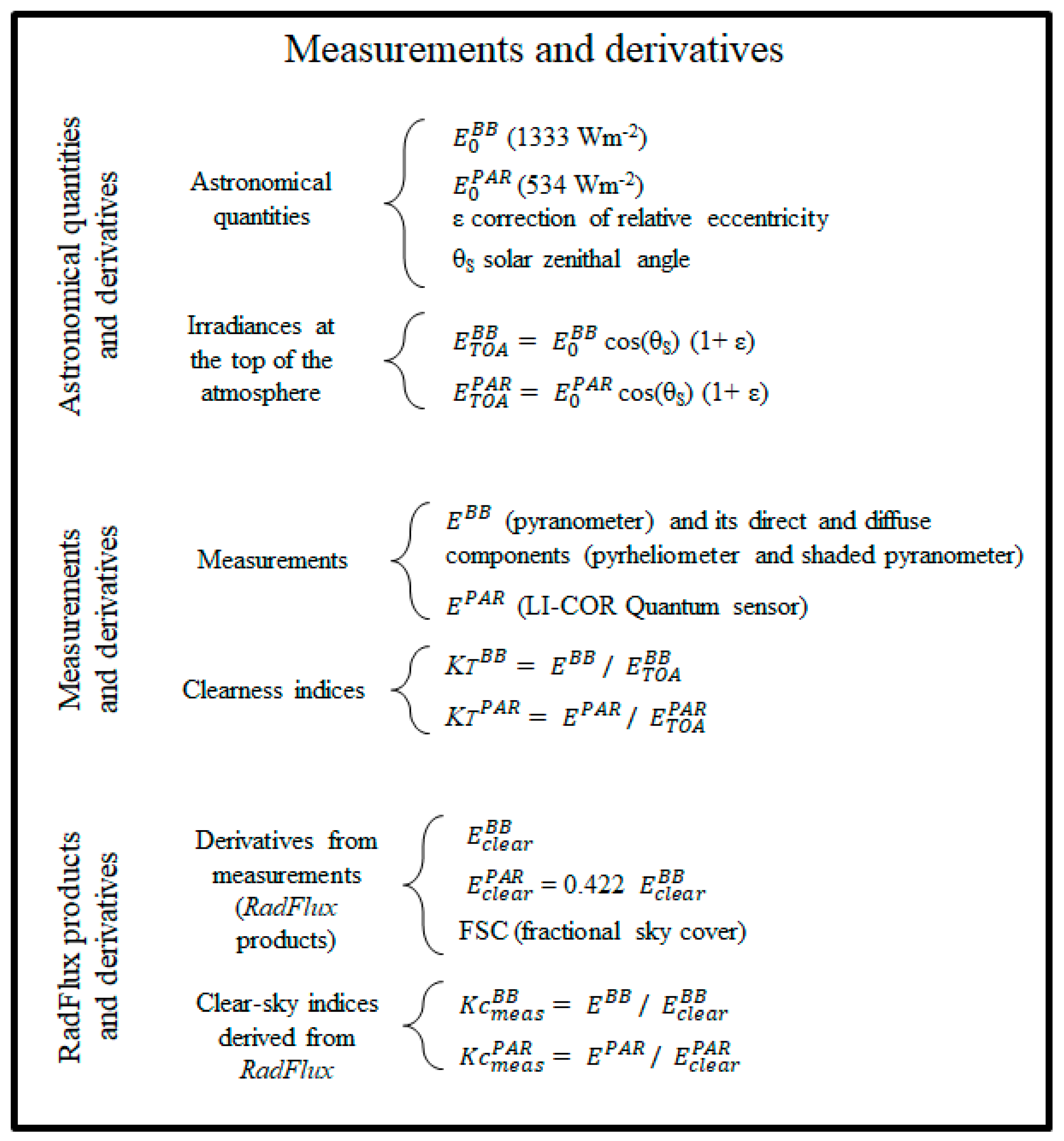
Other quantities were computed mostly for the purposes of validation. Astronomical quantities, namely the correction of relative eccentricity $\varepsilon$ and the solar zenithal angle θ_S, were obtained using the SG2 algorithm [62]. The yearly-averaged irradiances emitted by the sun and reaching the top of the atmosphere on a plane normal to the direction of the sun rays $E_0^{BB}$ and $E_0^{PAR}$ were calculated using a proper integration of the solar spectrum newGuey read from the libRadtran radiative transfer model [63,64] and then resampled to 5 nm and adjusted to the nominal total solar irradiance of 1361 W m⁻² as recommended by [65]. Thus, $E_0^{BB}$ was set to 1333 W m⁻² in the broadband range [280, 3000] nm, and its PAR fraction $E_0^{PAR}$ was set to 534 W m⁻². The irradiances $E_{TOA}^{BB}$ and $E_{TOA}^{PAR}$ at the top of the atmosphere were computed, as well as the clearness indices Kt^BB and Kt^PAR. Figure 2 provides an overview of the astronomical quantities, measurements, and their derivatives used in this study.

4. Analysis of the Relationships between ${\mathit{K}}_{\mathit{c}\_\mathit{m}\mathit{e}\mathit{a}\mathit{s}}^{\mathit{P}\mathit{A}\mathit{R}}$ and ${\mathit{K}}_{\mathit{c}\_\mathit{m}\mathit{e}\mathit{a}\mathit{s}}^{\mathit{B}\mathit{B}}$ for Different Cloudy Situations

At each station, for each year, the data set {$K_{c\_meas}^{PAR}$, $K_{c\_meas}^{BB}$} was split into five classes of cloudy situations:

• Class C1: 0.05 < FSC ≤ 0.30;
• Class C2: 0.30 < FSC ≤ 0.60;
• Class C3: 0.60 < FSC < 0.95;
• Class “any broken-cloud situation”: 0.05 < FSC < 0.95;
• Class “any cloudy situation” that comprises any cloudy situation whether overcast or broken: 0.05 < FSC ≤ 1.00.

The cloud cover becomes less and less fragmented from the C1 class to the C3 class. The splitting yielded five data subsets per year at each station. The same operation was performed but for all stations merged.

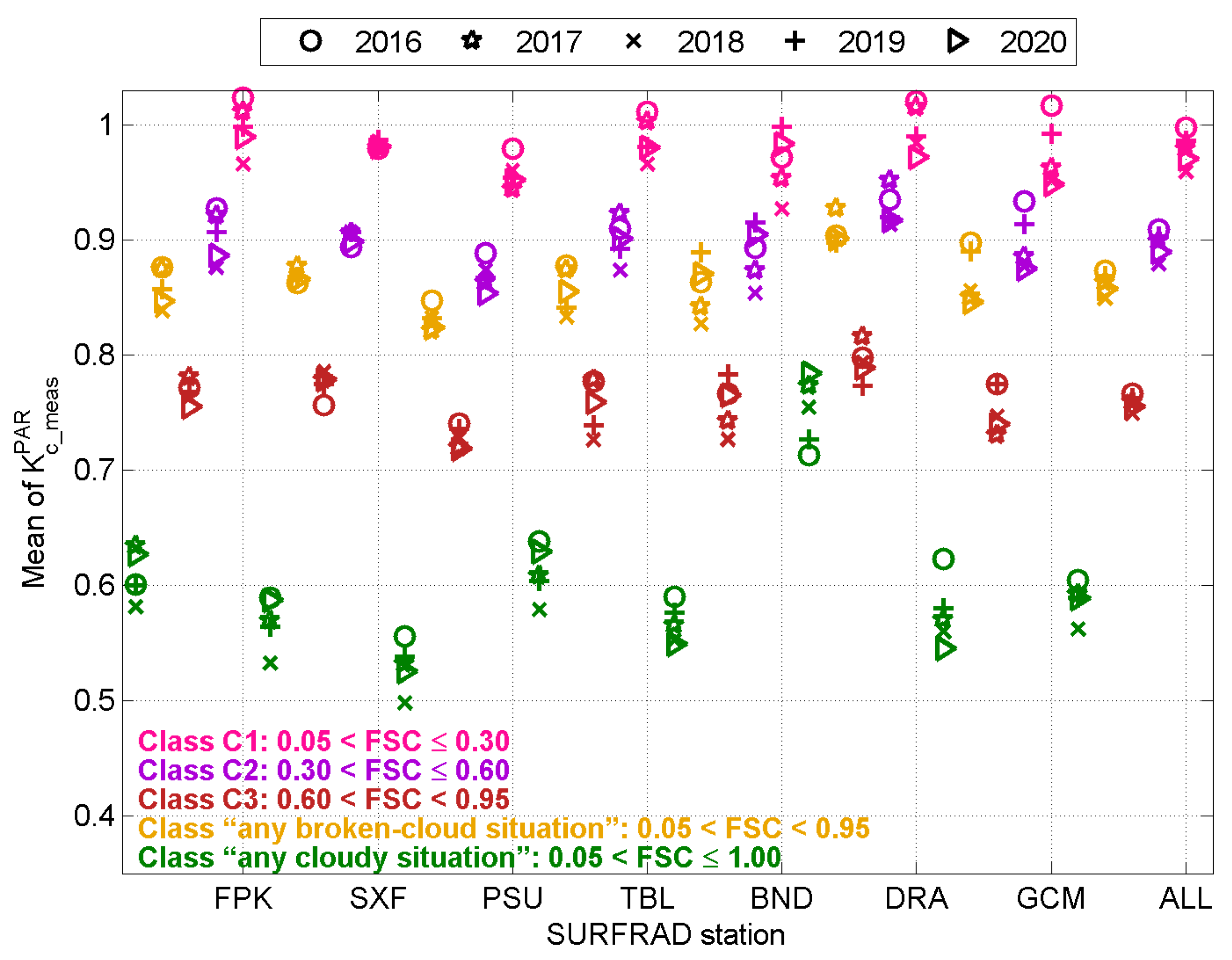
Figure 3 exhibits the mean of $K_{c\_meas}^{PAR}$ for each subset. As expected, the means for each subset vary with the year and the station, though in a limited manner, on the order of ±0.10. The means are the greatest for the C1 class (0.05 < FSC ≤ 0.30): they are greater than 0.9 and close to the clear-sky values. The means are around 0.90 for the C2 class (0.30 < FSC ≤ 0.60), 0.75 for the C3 class (0.60 < FSC < 0.95) and around 0.85 for the “any broken-cloud situation” class (0.05 < FSC ≤ 0.95). The smallest means are observed for the “any cloudy situation” class, which includes overcast conditions, and are less than 0.65 with the exception of Desert Rock (DRA), where the means range between 0.7 and 0.8.

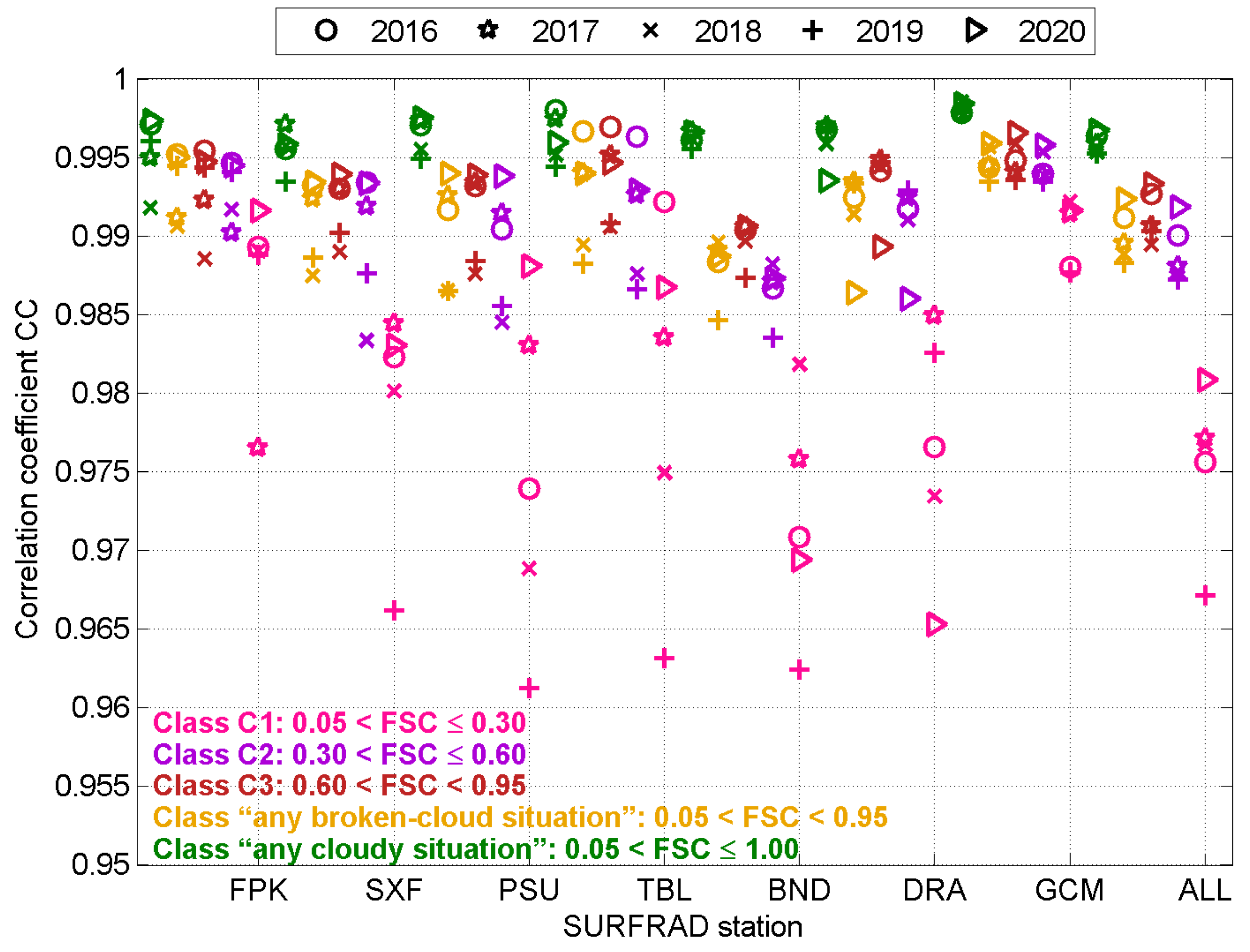
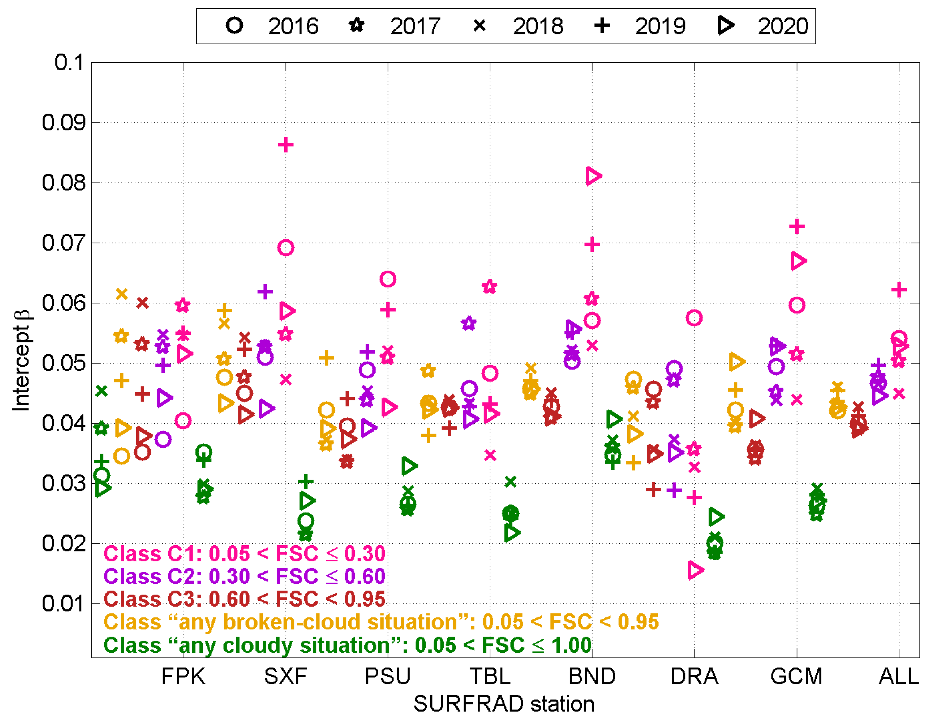
The correlation coefficients between $K_{c\_meas}^{PAR}$ and $K_{c\_meas}^{BB}$ were computed for each data subset and plotted in Figure 4. As a whole, they are greater than 0.96 whatever the subset, showing that $K_{c\_meas}^{PAR}$ and $K_{c\_meas}^{BB}$ are strongly related. The correlation coefficients are the smallest for the smallest FSC (C1 class), then for the C2 and C3 classes. The coefficients are greater than 0.99 for the “any cloudy situation” class. The least-squares fit between $K_{c\_meas}^{PAR}$ and $K_{c\_meas}^{BB}$ produced a series of affine functions, $K_{c\_fit}^{PAR}$ = α$K_{c\_meas}^{BB}$+β, which differ from one subset to another. Figure 5 and Figure 6 exhibit the slopes and intercepts for each subset. The slopes (Figure 5) range from 0.92 to 1.04; they are highly variable from station to station for a given year and a given class, from year to year for a given station and a given class, and from class to class for a given station and a given year. The intercepts (Figure 6) are also highly variable within the set of stations, the years, and the five classes. They range from 0.015 to 0.085 and, as a whole, are approximately 5% of the means of $K_{c\_meas}^{PAR}$ in each class.

From this first part of the study, it can be concluded that the broadband and PAR clear-sky indices are highly correlated, as expected, and are linked by affine functions whose parameters depend on the fractional sky cover, the year, and the site, in a manner that remains unclear presently. It is possible that we selected too large classes of FSC and that the use of the least-squares fitting technique may introduce some bias.

5. Testing the Accuracy of the WN2024 Model in Broken-Cloud Situations

Wandji Nyamsi et al. [50] proposed several linear relationships linking $K_c^{PAR}$ and $K_c^{BB}$ depending on the availability of cloud properties, namely cloud phase and cloud optical depth. Of particular interest here is their simplest model (Equation (5.4), p. 124) for cases where no information on clouds is available. The WN2024 model is as follows:

$$K_{c\_wn2024}^{PAR}=\left\{\begin{array}{c}1.058K_c^{BB}\mathrm{for}{K}_c^{BB}\le 1\\ 1.011K_c^{BB}\mathrm{for}{K}_c^{BB}>1\end{array}\right.$$

(4)

It was empirically established by using a very large number of simulations performed by means of the libRadtran radiative transfer model [63,64] in both clear and overcast conditions. Can the WN2024 model produce accurate estimates in the case of broken clouds? This is the subject of this section where the WN2024 model is assessed by comparing estimates from the application of this model against reference data.

The correlation coefficients between estimates and measurements were computed, as well as errors (estimates minus measurements) for each class of cloudy conditions at each station and for each year and all years merged, as well as for all stations merged for each year and all years merged. Errors were synthesized by the bias (mean of the errors), the standard deviation of errors, and the root mean square error (RMSE). Relative bias, standard deviation, and RMSE were computed with respect to the means of $K_{c\_meas}^{PAR}$. Least-squares fittings were performed, and slopes and intercepts were computed. The errors were also analyzed under various classes of FSC and solar zenithal angle. In addition, the comparison was also performed on a sixth class: FSC > 0.95, named “overcast”, which corresponds to the data set used in Wandji Nyamsi et al. [50] for overcast conditions. It is expected that the correlation coefficients and slopes of the fitting lines will both be close to 1. Biases are expected to be close to 0, as well as the standard deviations of errors and, hence, the RMSEs.

Table 3. Errors for each of the cloudy conditions, all stations merged and all years merged, for $K_c^{PAR}$.

	C1	C2	C3	Any Broken-Cloud	Any Cloudy	Overcast
FSC	]0.05, 0.30]	]0.30, 0.60]	]0.60, 0.95]	]0.05, 0.95]	]0.05, 1.00]	]0.95, 1.00]
Mean value	0.98	0.90	0.76	0.86	0.59	0.39
Correl. coeff.	0.966	0.986	0.990	0.988	0.995	0.995
Bias	0.02	0.02	0.01	0.01	0.00	0.00
Slope	0.96	1.00	1.01	1.00	1.02	1.02
Intercept	0.06	0.02	0.01	0.01	−0.01	−0.01
Standard dev.	0.04	0.04	0.04	0.04	0.03	0.03
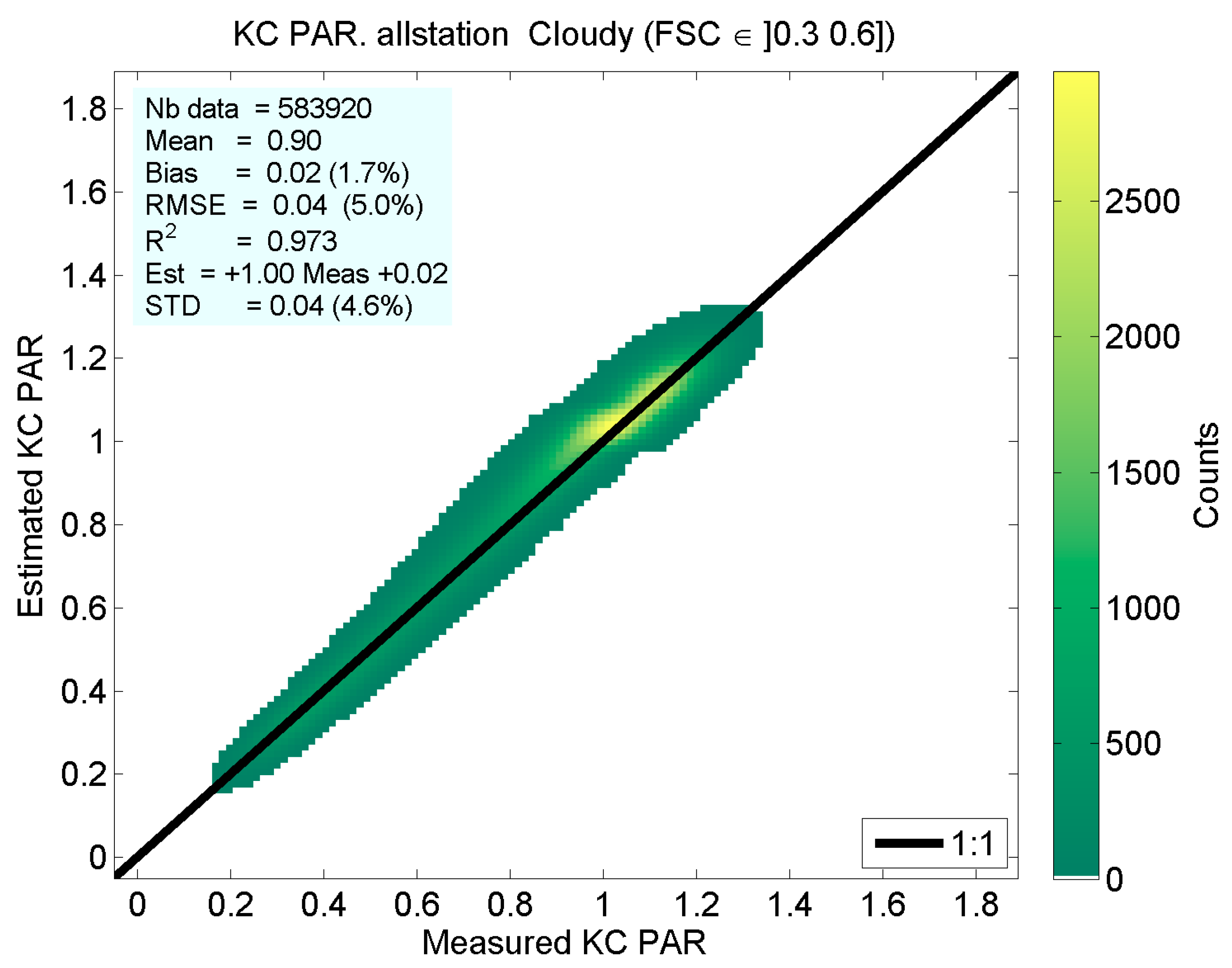
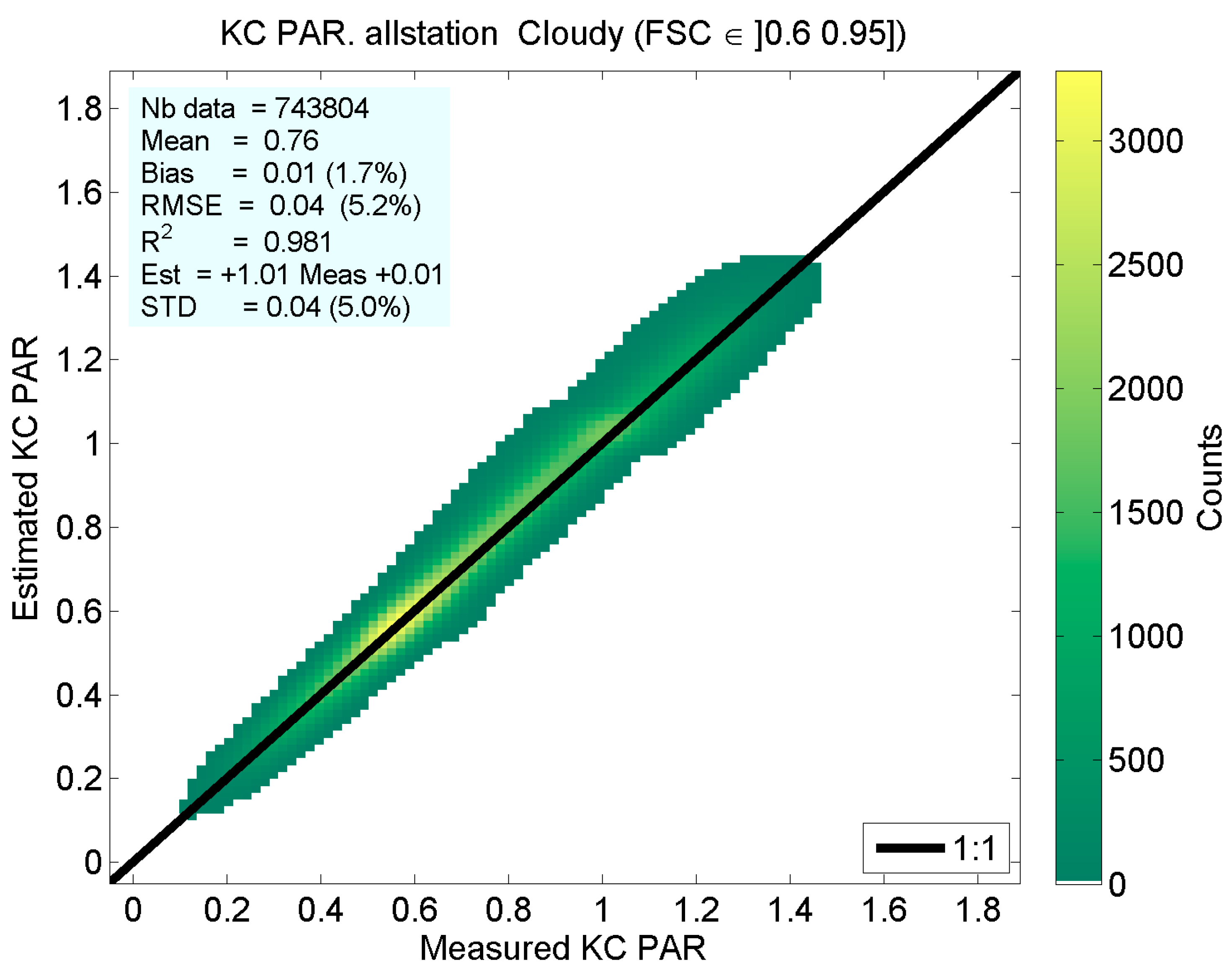
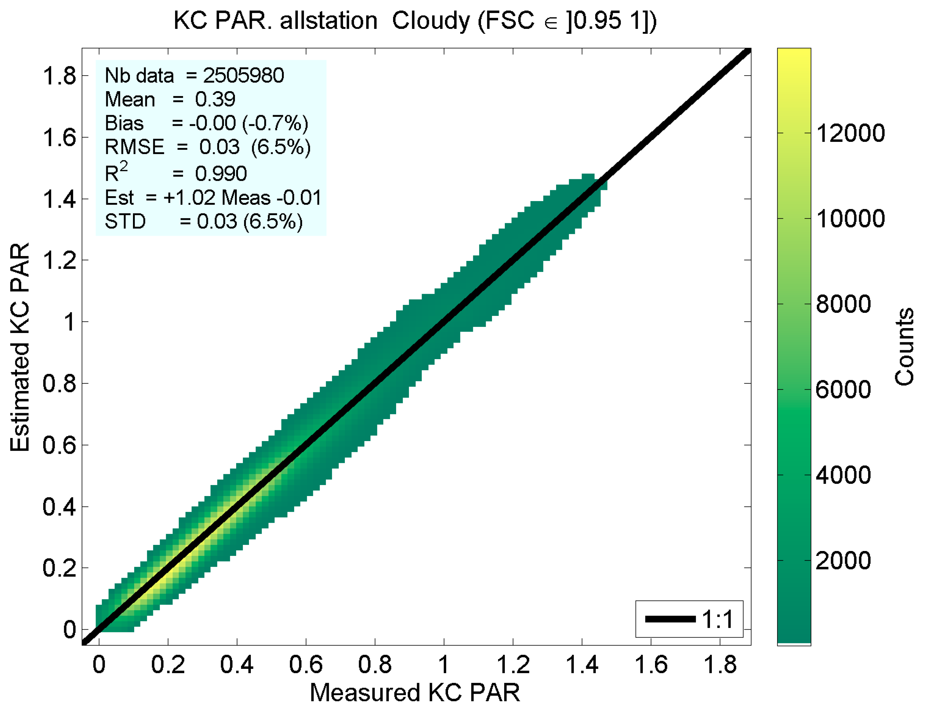
RMSE	0.04	0.04	0.04	0.04	0.03	0.03

gives the means, correlation coefficients, errors, and slopes of the fitting lines for each of the six classes with all stations merged for $K_c^{PAR}$. Figure 7, Figure 8, Figure 9, Figure 10, Figure 11 and Figure 12 exhibit the 2D histograms of measured $K_{c\_meas}^{PAR}$ and estimated $K_{c\_wn2024}^{PAR}$ for the six classes with all stations merged.

One observes that the 2D histograms exhibit a very good match between the estimates and measurements under all cloudy conditions. The points are well aligned along the 1:1 line with little scattering, and the slopes of the least-squares fitting lines are very close to 1. The errors made on $K_{c\_meas}^{PAR}$ are small (Table 3). For all stations merged, the bias ranges between 0.00 and 0.02. It is the smallest for the overcast class and increases as the FSC decreases. Similarly, the standard deviation of errors is the smallest for the overcast class (0.03) and rises to 0.04 for the C1 class. The relative RMSE ranges between 4.6% and 6.5%.

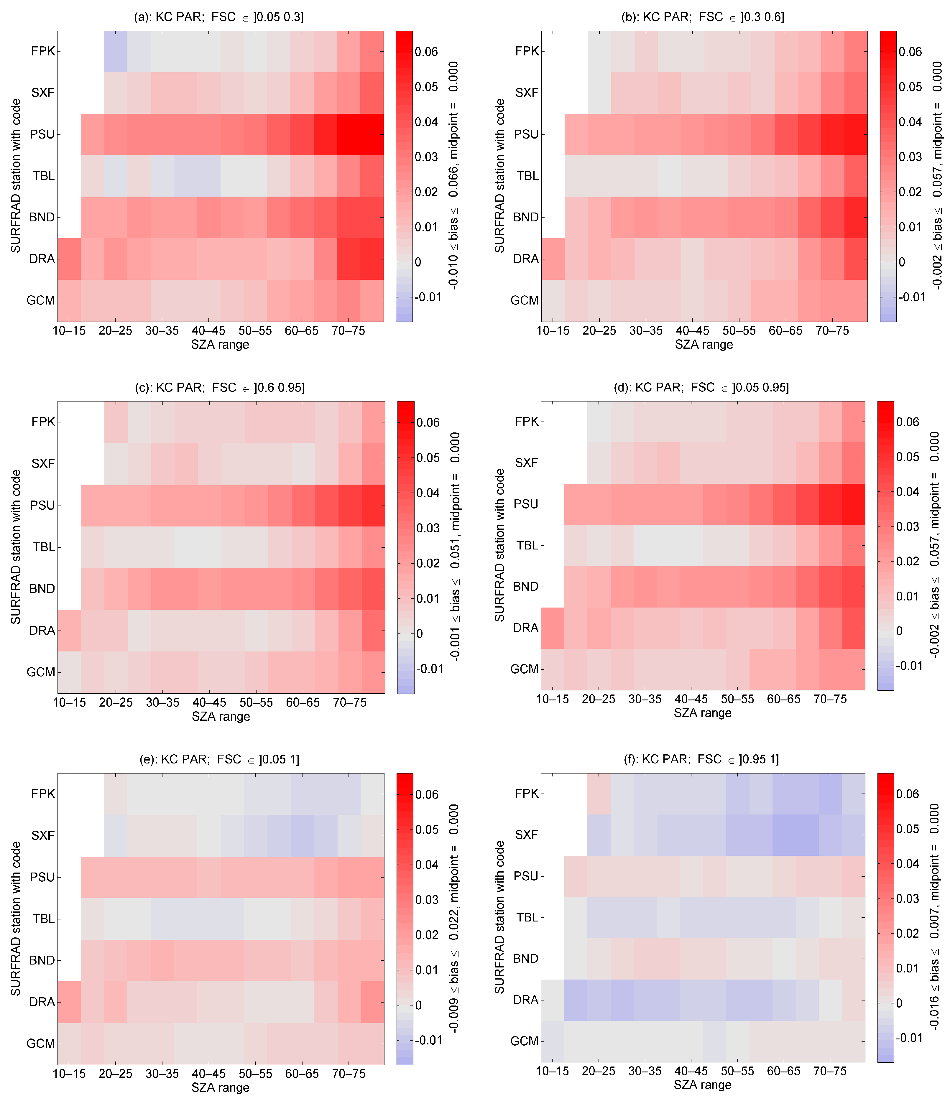
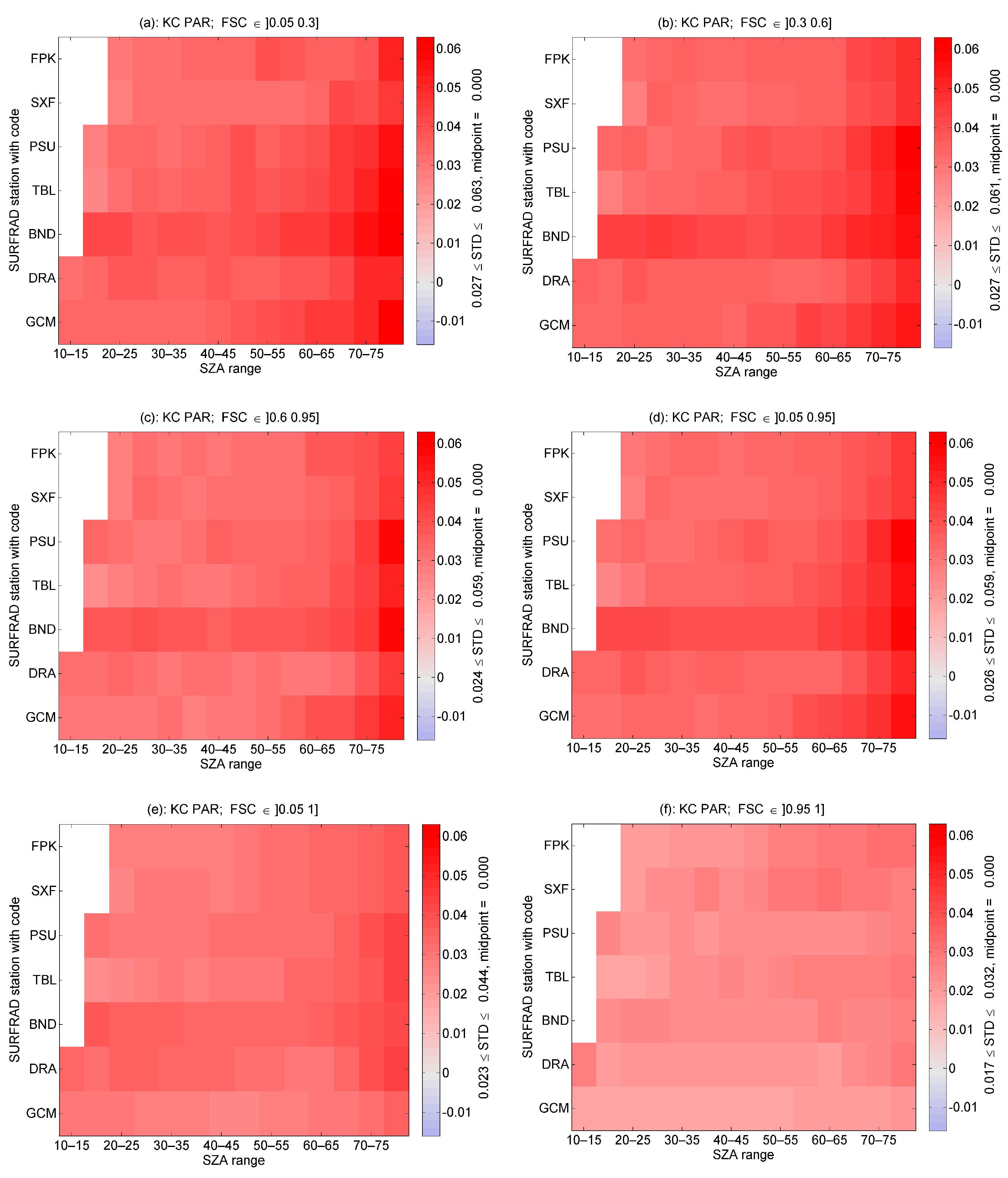
The bias exhibits slight changes with the station or the solar zenithal angle (Figure 13). It tends to increase as the solar zenithal angle increases above 60° for the C1, C2, C3, and any broken-cloud classes, and reach 0.03 as a whole, or 0.06 at stations Penn. State Univ. and Bondville. On the contrary, the standard deviations of the errors are fairly constant among stations and with changing solar zenithal angles (Figure 14).

These results demonstrate the good accuracy of the WN2024 model when applied to measurements from the SURFRAD network for any cloud conditions and broken-cloud conditions. De Blas et al. [31] also found that a single model may apply to the seven SURFRAD stations without significant loss.

6. Accuracy of the Combination of a Clear-Sky Model and the WN2024 Model in Any Cloudy Situation at SURFRAD Stations

In the previous section, the clear-sky PAR $E_{clear}^{PAR}$ was derived from the measurements themselves and, more precisely, from the clear-sky broadband irradiances $E_{clear}^{BB}$: $E_{clear}^{PAR}$ = (0.422 ± 0.006)$E_{clear}^{BB}$. It is a favorable case because the errors made on the modelling of $E_{clear}^{PAR}$ are limited. In this section, we address the case of using estimates of $E_{clear}^{PAR}$ that do not use ground-based measurements. Hence, this section offers another set of assessments, this time using a published PAR clear-sky model with its own uncertainties to independently evaluate $E_{clear}^{PAR}$.

The clear-sky model of Wandji Nyamsi et al. [38] was selected. It uses the most improved version of the k-distribution method and the correlated-k approximation [66,67], which is one of the schemes available in the libRadtran radiative transfer model, named “kato2andwandji” [65]. In this scheme, only 32 spectral bands over the large spectral range of [0.240, 4.606] µm are needed to calculate the broadband irradiance [66]. Wandji Nyamsi et al. [68] show that fluxes computed in the eleven spectral bands covering the PAR band are accurate. The eleven transmissivities taken from these eleven bands are spectrally resampled every 1 nm and then converted to fluxes. The resampled fluxes are aggregated over the PAR range [400, 700] nm, yielding the PAR fluxes. Similar approaches have been successfully applied to retrieve UV fluxes or daylight radiation [69,70]. The model uses as inputs the total column contents of ozone and water vapor, as well as the optical properties of aerosols provided by the Copernicus Atmosphere Monitoring Service (CAMS). Other variables are needed and are detailed in Wandji Nyamsi et al. [38]. Here, for simplicity and convenience, the retrieval of 1 min values of the inputs listed above was performed by machine-to-machine requests to the McClear web service on the Soda website [71] (www.soda-pro.com, accessed on 2 October 2022). Validation of the clear-sky model against SURFRAD measurements reveals similar or better performances than those of the Su et al. method [9]. The bias ranges from −3 to 13 W m⁻² (−1% to 5%), and the RMSE ranges from 8 to 18 W m⁻² (3% to 6%), depending on the station [38]. At all stations, the squared correlation is greater than 0.97. The relative values of the standard deviation are under 5%. If the statistical distribution of the errors is Gaussian, then the uncertainty (percentile 95) is under 10%, i.e., close to the uncertainty of the measurements (8%). Subsequently, when validating their own clear-sky model against the merging of all measurements performed in the SURFRAD network and another, Zhang et al. [12] reported similar performances: a squared correlation coefficient equal to 0.97, a bias of 2 W m⁻² (0.8%), and an RMSE of 18 W m⁻² (7.2%). These comparisons with ground-based measurements and similar works demonstrate the high quality of $E_{clear}^{PAR}$ using the Wandji Nyamsi et al. model [38].

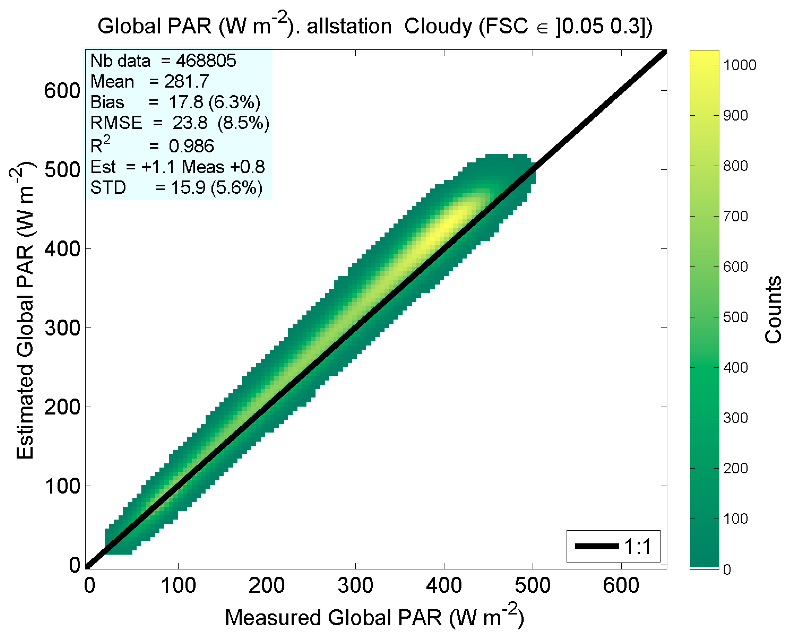
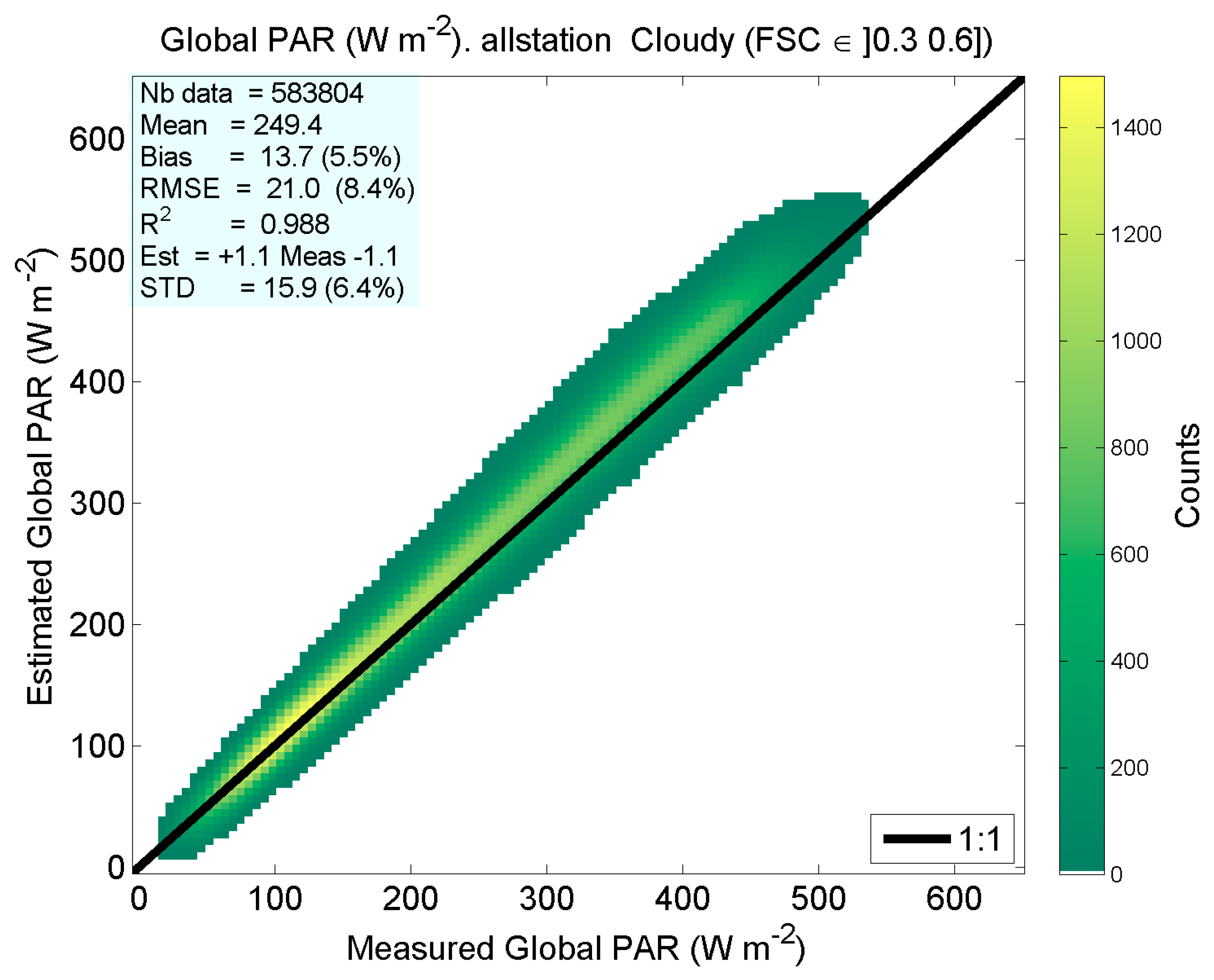
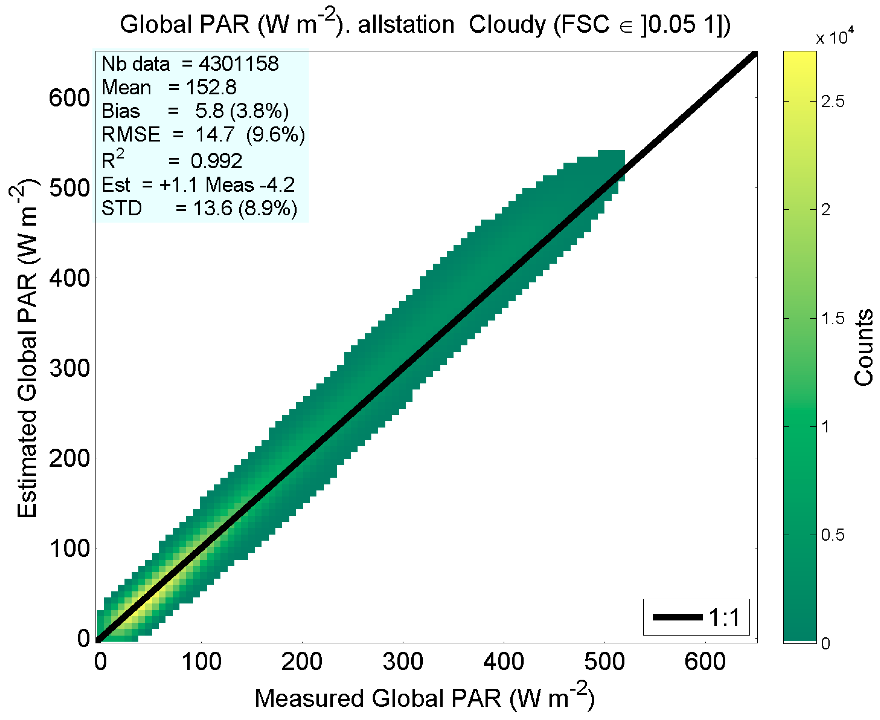
Next, $K_{c\_wn2024}^{PAR}$ obtained by Equation (4) is converted in $E_{WN2024}^{PAR}$ by using this new set of $E_{clear}^{PAR}$. As previously, the combination of the clear-sky model and the WN2024 model is assessed by comparing estimates against reference data. To better understand the results, three assessments are presented using the clear-sky index, the PAR, and the PAR clearness index, respectively. More precisely, the first assessment compares the estimates of $K_{c_{WN2024}}^{PAR}$ against $K_{c_{meas}}^{PAR}$, the second one deals with $E_{WN2024}^{PAR}$ against $E_{meas}^{PAR}$ and the third one with ${KT}_{WN2024}^{PAR}$ against ${KT}^{PAR}$. Relative bias, standard deviation, and RMSE were computed with respect to the means of $K_{c\_meas}^{PAR}$, $E_{meas}^{PAR}$, and ${KT}^{PAR}$. Figure 15, Figure 16, Figure 17, Figure 18, Figure 19 and Figure 20 exhibit the 2D histograms of measured PAR $E_{meas}^{PAR}$ and estimated PAR $E_{WN2024}^{PAR}$ for the six classes, all stations merged.

Table 4. Errors for each of the cloudy conditions, all stations merged and all years merged, for $K_c^{PAR}$ from the combination of a clear-sky model and the WN2024 model.

	C1	C2	C3	Any Broken-Cloud	Any Cloudy	Overcast
FSC	]0.05, 0.30]	]0.30, 0.60]	]0.60, 0.95]	]0.05, 0.95]	]0.05, 1.00]	]0.95, 1.00]
Mean value	0.94	0.87	0.74	0.83	0.58	0.39
Correl. Coeff.	0.944	0.977	0.980	0.978	0.990	0.987
Bias	0.06	0.04	0.03	0.04	0.02	0.00
Slope	0.99	1.03	1.02	1.03	1.05	1.01
Intercept	0.07	0.02	0.02	0.01	−0.02	−0.01
Standard dev.	0.05	0.06	0.05	0.06	0.05	0.04
RMSE	0.08	0.07	0.06	0.06	0.05	0.04

,

Table 5. Errors for each of the cloudy conditions, all stations merged and all years merged, for $E^{PAR}$ (in W m⁻²) from the combination of a clear-sky model and the WN2024 model.

	C1	C2	C3	Any Broken-Cloud	Any Cloudy	Overcast
FSC	]0.05, 0.30]	]0.30, 0.60]	]0.60, 0.95]	]0.05, 0.95]	]0.05, 1.00]	]0.95, 1.00]
Mean value	281.7	249.4	198.2	236.6	152.8	92.7
Correl. Coeff.	0.993	0.994	0.993	0.994	0.996	0.994
Bias	17.8	13.7	8.9	12.8	5.8	0.8
Slope	1.1	1.1	1.1	1.1	1.1	1.0
Intercept	0.8	−1.1	−1.7	−1.8	−4.2	−3.3
Standard dev.	15.9	15.9	13.9	15.5	13.6	9.1
RMSE	23.8	21.0	16.5	20.1	14.7	9.1

and

Table 6. Errors for each of the cloudy conditions, all stations merged and all years merged, for ${KT}^{PAR}$ from the combination of a clear-sky model and the WN2024 model.

	C1	C2	C3	Any Broken-Cloud	Any Cloudy	Overcast
FSC	]0.05, 0.30]	]0.30, 0.60]	]0.60, 0.95]	]0.05, 0.95]	]0.05, 1.00]	]0.95, 1.00]
Mean value	0.79	0.72	0.61	0.69	0.47	0.32
Correl. Coeff.	0.963	0.982	0.984	0.982	0.992	0.989
Bias	0.05	0.04	0.02	0.03	0.01	0.00
Slope	1.03	1.05	1.04	1.05	1.06	1.03
Intercept	0.03	0.00	0.00	−0.00	−0.02	−0.01
Standard dev.	0.04	0.04	0.04	0.04	0.04	0.03
RMSE	0.06	0.06	0.05	0.06	0.04	0.03

give the means, correlation coefficients, errors, and slopes of the fitting lines for each of the six classes, all stations merged, for $K_c^{PAR}$, $E^{PAR}$ and ${KT}^{PAR}$, respectively.

Figure 15, Figure 16, Figure 17, Figure 18, Figure 19 and Figure 20 show that the estimates are close to the measurements and fairly well aligned along the 1:1 line, with limited scattering in all the cloudy conditions. One may note a tendency to overestimate the PAR at values greater than 350 W m⁻². This is confirmed by the values of the slopes reported in Table 5, which are equal to 1.1, except for the overcast conditions where the slope is 1.0. This overestimation of the greatest values is also observed in $K_c^{PAR}$ and ${KT}^{PAR}$ with slopes greater than 1.00 in most cases (Table 4 and Table 6). The correlation coefficients are large for all variables and all cloudy conditions, greater than 0.99 for $E^{PAR}$, 0.94 for $K_c^{PAR}$, and 0.96 for ${KT}^{PAR}$.This tendency has been discussed in [38] and is possibly related to the assumed PAR-albedo computed with a constant of 0.47, which, realistically, should depend on the type of surface.

The results are very good in overcast conditions: the bias is equal to 0.8 W m⁻² for $E^{PAR}$, 0.00 for $K_c^{PAR}$ (Table 4) and 0.00 for ${KT}^{PAR}$ (Table 6). The slopes are, respectively, 1.0, 1.01, and 1.03, and the standard deviations of errors are, respectively, 9.1 W m⁻², 0.04, and 0.03. The RMSE for $E^{PAR}$ is 9 W m⁻² and is similar to the RMSE ranging from 4 to 6 W m⁻² reported by de Blas et al. [31] (read from their Figure 8) when testing several models after calibration against the SURFRAD measurements.

The results are less good in other cloudy conditions and, as a whole, worsen as the FSC decreases, i.e., when fewer and fewer scattered clouds are present. The bias for $E^{PAR}$ increases from 8.9 W m⁻² for class C3 to 17.8 W m⁻² for class C1 when the FSC is small ]0.05, 0.30]. The standard deviation of errors increases from 13.9 W m⁻² for class C3 to 15.9 W m⁻² for class C1. When all cloudy conditions are merged (any cloud), the bias, standard deviation, and RMSE are, respectively, 5.8, 13.6, and 14.7 W m⁻².

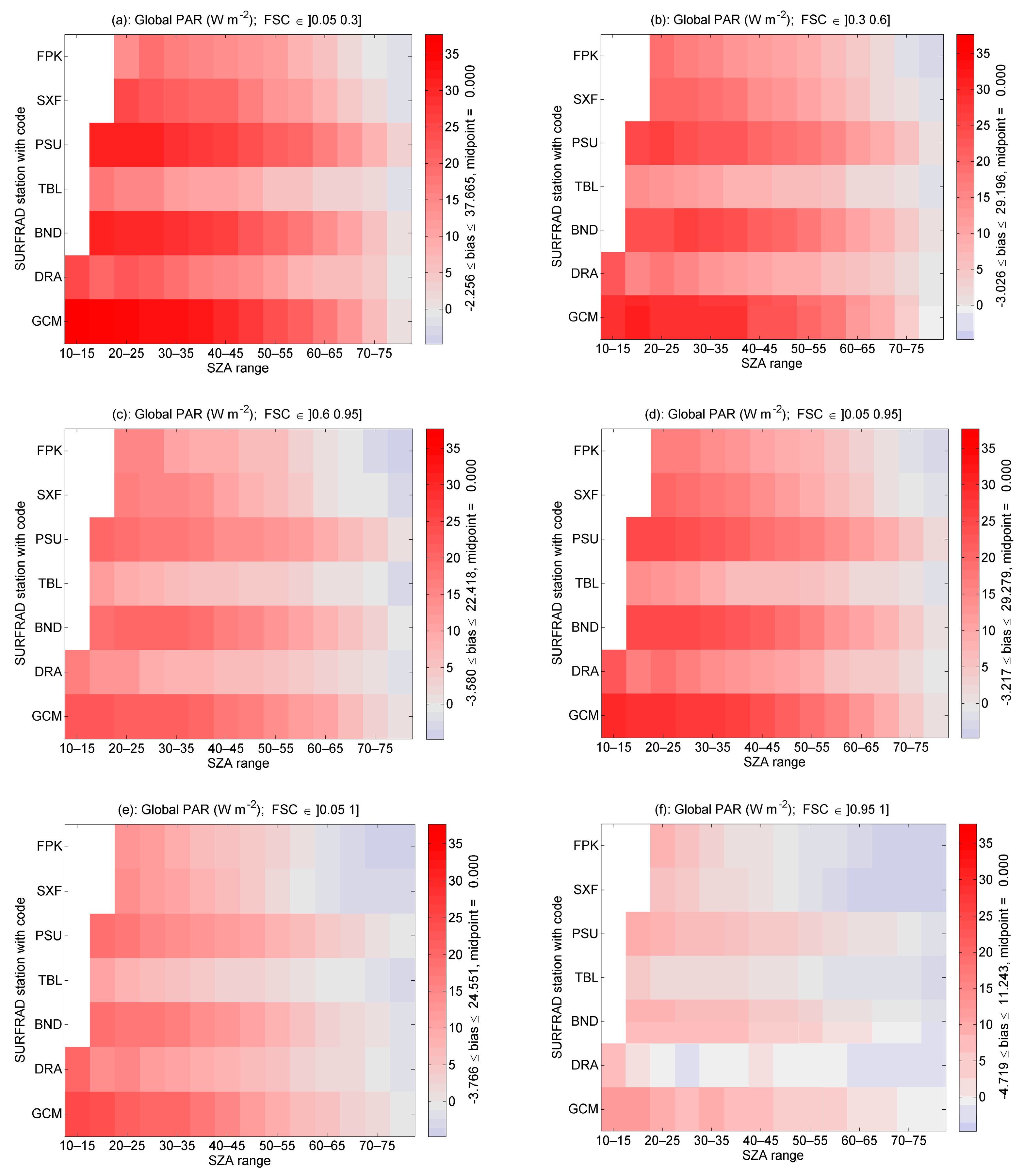
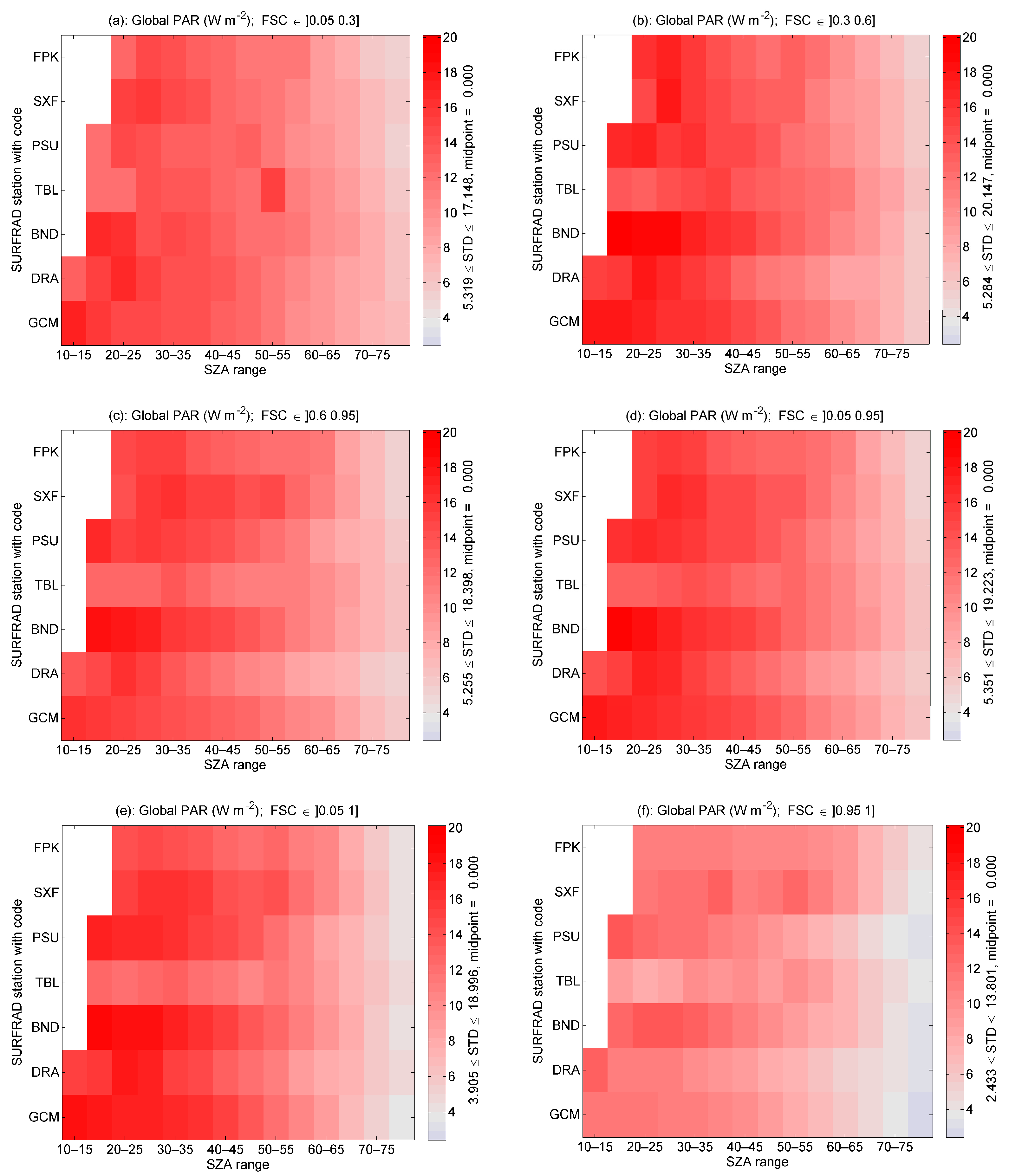
The bias for $E^{PAR}$ exhibits slight changes with the station or the solar zenithal angle (Figure 21). It tends to increase as the solar zenithal angle decreases for the any broken-cloud, C1, C2, and C3 classes. On the contrary, the standard deviations of the errors for $E^{PAR}$ are fairly constant among stations and with changing solar zenithal angles (Figure 22).

7. Discussion

Relationships between PAR and broadband clear-sky indices have been assessed here under broken-cloud and any cloudy conditions using appropriate ground-based measurements. Both indices are highly correlated, as expected. The PAR clear-sky index can be accurately expressed by an affine function of the broadband clear-sky index. The parameters of the function depend on the fractional sky cover, on the year, and on the site, in a manner that remains unclear presently. A possible track for explanation is the modeling of the ground reflective properties, which here are excerpted from the MODIS-derived data sets of BRDF parameters [72] used by the McClear web service. It is likely that changes in reflective properties in the PAR range are not properly accounted for in our models and may partly explain the results.

The first objective of the study is unachieved, as no accurate linear function could be extracted from these comparisons, contrary to the case of overcast conditions. A linear function is preferable to an affine function because it ensures that $E^{PAR}$ is null when $E^{BB}$ is null.

The linear WN2024 model provides fairly good results in any cloudy situation; the correlation coefficients are very large, and the scattering is limited, showing the ability of this model combined with the clear-sky model of Wandji Nyamsi et al. [38] to reproduce the variability of the measurements. This combination of models tends to overestimate the greatest PAR above 350 W m⁻². Accuracy is still far from the accuracy of the measurements: the relative bias ranges from 1% to 6%, and the relative RMSE ranges from 8 to 10%.

Nevertheless, our results for $E^{PAR}$ under any cloudy condition compare favorably with other works, which also found that a single model is sufficient for the seven SURFRAD stations and that performances decrease in cloudy conditions compared to clear-sky conditions [13,31]. For the same SURFRAD stations, Tang et al. [13] reported a bias of 6 W m⁻², an RMSE of 44 W m⁻², and a correlation coefficient of 0.94, which are comparable to ours: 6 W m⁻² (4% of the mean of $E^{PAR}$), 15 W m⁻² (10%), and 0.996, respectively.

When testing several models after calibration against the SURFRAD measurements, De Blas et al. [31] found RMSEs ranging from 8 to 11 W m⁻² (4 to 5% relative to the mean of $E^{PAR}$) depending on the model relative to the mean $E^{PAR}$. These values are better than ours: 15 W m⁻² (10%). This difference illustrates the benefit of calibrating empirical models against ground measurements and, at the same time, underlines the geographical limits of such methods.

Zhang et al. [12] dealt with measurements from two networks, including SURFRAD. They also found that the performance of their all-sky model was better in clear-sky conditions than in cloudy conditions. They reported a bias of 2 W m⁻², an RMSE of 51 W m⁻², and a correlation coefficient of 0.91 for cloudy conditions, and 2 W m⁻², 44 W m⁻², and 0.93 in all-sky conditions.

Thomas et al. [32] tested five published uncalibrated methods applied to broadband irradiances derived from satellite images against ground-based measurements performed at 33 sites located in the field of view of the MSG-prime satellites. They found that performances are better in clear-sky conditions than in cloudy situations. They reported relative biases ranging from 1% to 23%, relative RMSEs ranging from 25% to 36%, and correlation coefficients around 0.955. They also tested the PAR product available from the SARAH-3 data set [22] and found a relative bias of 9%, a relative RMSE of 27%, and a correlation coefficient of 0.954. These results in [32] are worse than those given above, but it should be taken into account that they include the uncertainty of these satellite-based models in estimating $E^{BB}$.

The role of the FSC in the assessment of $E^{PAR}$ from $E^{BB}$ is evidenced by the dependance of errors with the FSC and cannot be neglected. It is believed that more sophisticated models must be developed to better account for broken-cloud conditions in order to obtain better estimates of PAR. Contrary to expectations, this study has not provided good insights on how estimates of the fraction of pixel covered by clouds provided by analysis of satellite images could be exploited to improve the retrieval of PAR in broken-cloud conditions. Advanced techniques based on machine learning techniques and, more generally, on artificial intelligence would have likely provided a model able to accurately reproduce $E^{PAR}$ in any conditions. Such models require training on data sets, and this may impede the worldwide applicability of the models.

The present study has practical implications, as it shows that the WN2024 model is efficient, useful, and easy to implement for deriving the PAR clear-sky index from the broadband clear-sky index, even in broken-cloud conditions. Because the present work is entirely based on the analysis of ground-based measurements, it therefore exhibits limits in its geographical and temporal coverages. At first glance, it therefore may contradict the claim for worldwide applicability of the WN2024 model, but it must be recalled that the WN2024 model has been validated against a large number of RTM situations covering many geographical and climatic situations. Therefore, it is believed to be applicable worldwide with the same level of accuracy, and it is further believed that there is no need for local calibration. The authors are aware that they have no strong evidence to support this claim and recognize that potential limitations may exist when current cloud conditions have not been represented or have been inaccurately represented in the very large set of RTM simulations.

The application of the WN2024 model requests two clear-sky models, one for broadband irradiance and another one for PAR. Once these two models are established, their combination with the WN2024 model may apply to any measurement or estimate of the broadband irradiance $E^{BB}$ to derive $E^{PAR}$, whether $E^{BB}$ originates from measurements, satellite-based retrievals, or meteorological reanalysis. As several popular methods for retrieving $E^{BB}$ from satellite images use a so-called cloud index, or cloud effective albedo, that is directly related to the clear-sky index, they can be easily tuned into methods for estimating $E^{PAR}$ by using the WN2024 model and a PAR clear-sky model.

Our study does not deal with the direct and diffuse components of the PAR. These components are of utmost importance for accurate assessments of the radiation that reaches foliage in dense vegetation, algae in water, or vegetation in agriphotovoltaics. Estimating these components is the next track for research [4]. Several elements are already available and may help. The clear-sky model for PAR from Wandji Nyamsi et al. [38] includes its direct component and thus the diffuse part, and Wandji Nyamsi et al. [50] found that the PAR and broadband clear-sky indices were equal under any sky homogeneous conditions for the direct component. Once the PAR and its direct component are computed, the diffuse component is easily obtained.

8. Conclusions

The results demonstrate that clear-sky indices in the photosynthetically active radiation (PAR) range and broadband clear-sky indices are highly correlated in broken-cloud conditions using ground-based measurements obtained from the Surface Radiation Budget Network in the U.S.A. mainland. The indices are linked by affine functions whose parameters depend on the fractional sky cover (FSC), year, and site.

The WN2024 model relates both indices in a linear manner and has been validated against this same set of measurements and a great deal of RTM simulations. It was found that this model is also efficient in broken-cloud conditions with the same level of accuracy as in overcast conditions. This model can be combined with another model providing estimates of the PAR in clear-sky conditions to yield the PAR in any conditions.

When the PAR clear-sky model of [38] is used in combination with the WN2024 model, it was found that the result tends to overestimate the PAR measured at the SURFRAD stations as the FSC decreases, i.e., when fewer and fewer scattered clouds are present. The bias is equal to 1 W m⁻² in overcast conditions, up to 18 W m⁻² when the FSC is small, and 6 W m⁻² when all cloudy conditions are merged. The RMSEs are 5, 24, and 15 W m⁻², respectively. This may be different from other PAR clear-sky models.

Because of the robustness of our models, we find that the linear WN2024 and the clear-sky models can be combined with estimates of the broadband irradiance from satellites to yield estimates of PAR globally.

References

1. McCree, K.J. Test of current definitions of photosynthetically active radiation against leaf photosynthesis data. Agric. For. Meteorol. 1972, 10, 443–453. [Google Scholar] [CrossRef]
2. Akitsu, T.; Kume, A.; Hirose, Y.; Ijima, O.; Nasahara, K.N. On the stability of radiometric ratios of photosynthetically active radiation to global solar radiation in Tsukuba, Japan. Agric. For. Meteorol. 2015, 209–210, 59–68. [Google Scholar] [CrossRef]
3. Nwokolo, S. A global review of empirical models for estimating photosynthetically active radiation. Trends Renew. Energy 2018, 4, 236–327. [Google Scholar] [CrossRef]
4. Musleh, Y.J.K.; Rahman, T. Predictive models for photosynthetic active radiation irradiance in temperate climates. Renew. Sustain. Energy Rev. 2024, 200, 114599. [Google Scholar] [CrossRef]
5. LI-190R Quantum Sensor. Available online: https://www.licor.com/env/products/light/quantum.html (accessed on 15 March 2024).
6. Pinker, R.T.; Laszlo, I. Global distribution of photosynthetically active radiation as observed from satellites. J. Clim. 1992, 5, 56–65. Available online: www.jstor.org/stable/26197041 (accessed on 20 June 2024). [CrossRef]
7. Frouin, R.; Pinker, R.T. Estimating photosynthetically active radiation (PAR) at the Earth’s surface from satellite observations. Remote Sens. Environ. 1995, 51, 98–107. [Google Scholar] [CrossRef]
8. Frouin, R.; Murakami, H. Estimating photosynthetically available radiation at the ocean surface from ADEOS-II global imager data. J. Oceanogr. 2007, 63, 493–503. [Google Scholar] [CrossRef]
9. Su, W.; Charlock, T.P.; Rose, F.G.; Rutan, D. Photosynthetically active radiation from Clouds and the Earth’s Radiant Energy System (CERES) products. J. Geophys. Res. Biogeosci. 2007, 112, G02022. [Google Scholar] [CrossRef]
10. Müller, R.; Behrendt, T.; Hammer, A.; Kemper, A. A new algorithm for the satellite-based retrieval of solar surface irradiance in spectral bands. Remote Sens. 2012, 4, 622–647. [Google Scholar] [CrossRef]
11. Vindel, J.M.; Valenzuela, R.X.; Navarro, A.A.; Zarzalejo, L.F.; Paz-Gallardo, A.; Souto, J.A.; Méndez-Gómez, R.; Cartelle, D.; Casares, J.J. Modeling photosynthetically active radiation from satellite-derived estimations over mainland Spain. Remote Sens. 2018, 10, 849. [Google Scholar] [CrossRef]
12. Zhang, H.; Dong, X.; Xi, B.; Xin, X.; Liu, Q.; He, H.; Xie, X.; Li, L.; Yu, S. Retrieving high-resolution surface photosynthetically active radiation from the MODIS and GOES-16 ABI data. Remote Sens. Environ. 2021, 260, 112436. [Google Scholar] [CrossRef]
13. Tang, W.; Qin, J.; Yang, K.; Jiang, Y.; Pan, W. Mapping long-term and high-resolution global gridded photosynthetically active radiation using the ISCCP H-series cloud product and reanalysis data. Earth Syst. Sci. Data 2022, 14, 2007–2019. [Google Scholar] [CrossRef]
14. Nwokolo, S.C.; Ogbulezie, J.C.; Obiwulu, A.U. Impacts of climate change and meteo-solar parameters on Photosynthetically Active Radiation prediction using hybrid machine learning with physics-based models. Adv. Space Res. 2022, 70, 3614–3637. [Google Scholar] [CrossRef]
15. Pfeifroth, U.; Kothe, S.; Müller, R.; Trentmann, J.; Hollmann, R.; Fuchs, P.; Werscheck, M. Surface Radiation Data Set—Heliosat (SARAH)—Edition 2. Satellite Application Facility on Climate Monitoring: Darmstadt, Germany, 2017. [Google Scholar] [CrossRef]
16. Qu, Z.; Oumbe, A.; Blanc, P.; Espinar, B.; Gesell, G.; Gschwind, B.; Klüser, L.; Lefèvre, M.; Saboret, L.; Schroedter-Homscheidt, M.; et al. Fast radiative transfer parameterisation for assessing the surface solar irradiance: The Heliosat-4 method. Meteorol. Z. 2017, 26, 33–57. [Google Scholar] [CrossRef]
17. Müller, R.; Pfeifroth, U. Remote sensing of solar surface radiation—A reflection of concepts, applications and input data based on experience with the effective cloud albedo. Atmos. Meas. Tech. 2022, 15, 1537–1561. [Google Scholar] [CrossRef]
18. Chen, S.; Li, C.; Xie, Y.; Li, M. Global and direct solar irradiance estimation using deep learning and selected spectral satellite images. Appl. Energy 2023, 352, 121979. [Google Scholar] [CrossRef]
19. Aradpour, S.; Deng, Z. Remote sensing algorithm for retrieving global-scale sea surface solar irradiance. Environ. Monit. Assess. 2023, 195, 1355. [Google Scholar] [CrossRef]
20. Huang, C.; Shi, H.; Yang, D.; Gao, L.; Zhang, P.; Fu, D.; Xia, X.; Chen, Q.; Yuan, Y.; Liu, M.; et al. Retrieval of sub-kilometer resolution solar irradiance from Fengyun-4A satellite using a region-adapted Heliosat-2 method. Sol. Energy 2023, 264, 112038. [Google Scholar] [CrossRef]
21. Verbois, H.; Saint-Drenan, Y.-M.; Becquet, V.; Gschwind, B.; Blanc, P. Retrieval of surface solar irradiance from satellite imagery using machine learning: Pitfalls and perspectives. Atmos. Meas. Tech. 2023, 16, 4165–4181. [Google Scholar] [CrossRef]
22. Pfeifroth, U.; Drücke, J.; Kothe, S.; Trentmann, J.; Schröder, M.; Hollmann, R. SARAH-3—Satellite-based climate data records of surface solar radiation. Earth Syst. Sci. Data Discuss. 2024, 1–28. [Google Scholar] [CrossRef]
23. Boilley, A.; Wald, L. Comparison between meteorological re-analyses from ERA-Interim and MERRA and measurements of daily solar irradiation at surface. Renew. Energy 2015, 75, 135–143. [Google Scholar] [CrossRef]
24. Kobayashi, S.; Ota, Y.; Harada, Y.; Ebita, A.; Moriya, M.; Onoda, H.; Onogi, K.; Kamahori, H.; Kobayashi, C.; Endo, H.; et al. The JRA-55 reanalysis: General specifications and basic characteristics. J. Meteorol. Soc. Jpn. 2015, 93, 5–48. [Google Scholar] [CrossRef]
25. Hersbach, H.; Dee, D. ERA5 reanalysis is in production. ECMWF Newsl. 2016, 147, 7. [Google Scholar]
26. Gelaro, R.; McCarty, W.; Suárez, M.J.; Todling, R.; Molod, A.; Takacs, L.; Randles, C.A.; Darmenov, A.; Bosilovich, M.G.; Reichle, R.; et al. The modern-era retrospective analysis for research and applications, Version 2 (MERRA-2). J. Clim. 2017, 30, 5419–5454. [Google Scholar] [CrossRef]
27. Liu, C.; Allan, R.P.; Mayer, M.; Hyder, P.; Loeb, N.G.; Roberts, C.D.; Valdivieso, M.; Edwards, J.M.; Vidale, P.-L. Evaluation of satellite and reanalysis based global net surface energy flux and uncertainty estimates. J. Geophys. Res. Atmos. 2017, 122, 6250–6272. [Google Scholar] [CrossRef]
28. Trolliet, M.; Walawender, J.P.; Bourlès, B.; Boilley, A.; Trentmann, J.; Blanc, P.; Lefèvre, M.; Wald, L. Estimating downwelling solar irradiance at the surface of the tropical Atlantic Ocean: A comparison of PIRATA measurements against several re-analyses and satellite-derived data sets. Ocean. Sci. 2018, 14, 1021–1056. [Google Scholar] [CrossRef]
29. Yang, D.; Bright, J.M. Worldwide validation of 8 satellite-derived and reanalysis solar radiation products: A preliminary evaluation and overall metrics for hourly data over 27 years. Sol. Energy 2020, 210, 3–19. [Google Scholar] [CrossRef]
30. Thomas, C.; Dorling, S.; Wandji Nyamsi, W.; Wald, L.; Rubino, S.; Saboret, L.; Trolliet, M.; Wey, E. Assessment of five different methods for the estimation of surface photosynthetically active radiation from satellite imagery at three sites—Application to the monitoring of indoor soft fruit crops in southern UK. Adv. Sci. Res. 2019, 16, 229–240. [Google Scholar] [CrossRef]
31. de Blas, M.; García-Rodríguez, A.; García, I.; Torres, J.L. Validation and calibration of models to estimate photosynthetically active radiation considering different time scales and sky conditions. Adv. Space Res. 2022, 70, 1737–1760. [Google Scholar] [CrossRef]
32. Thomas, C.; Wandji Nyamsi, W.; Arola, A.; Pfeifroth, U.; Trentmann, J.; Dorling, S.; Laguarda, A.; Fischer, M.; Aculinin, A. Smart approaches for evaluating photosynthetically active radiation at various stations based on MSG prime satellite imagery. Atmosphere 2023, 14, 1259. [Google Scholar] [CrossRef]
33. Ferrera-Cobos, F.; Vindel, J.M.; Valenzuela, R.X.; González, J.A. Models for estimating daily photosynthetically active radiation in oceanic and Mediterranean climates and their improvement by site adaptation techniques. Adv. Space Res. 2020, 65, 1894–1909. [Google Scholar] [CrossRef]
34. García-Rodríguez, A.; García-Rodríguez, S.; Granados-López, D.; Díez-Mediavilla, M.; Alonso-Tristán, C. Extension of PAR models under local all-sky conditions to different climatic zones. Appl. Sci. 2022, 12, 2372. [Google Scholar] [CrossRef]
35. Bosch, J.L.; López, G.; Batlles, F.J. Global and direct photosynthetically active radiation parameterizations for clear-sky conditions. Agric. For. Meteorol. 2009, 149, 146–158. [Google Scholar] [CrossRef]
36. Wang, L.; Gong, W.; Feng, L.; Lin, A.; Hu, B.; Zhou, M. Estimation of hourly and daily photosynthetically active radiation in Inner Mongolia, China, from 1990 to 2012. Int. J. Climatol. 2015, 35, 3120–3131. [Google Scholar] [CrossRef]
37. Wandji Nyamsi, W.; Espinar, B.; Blanc, P.; Wald, L. Estimating the photosynthetically active radiation under clear skies by means of a new approach. Adv. Sci. Res. 2015, 12, 5–10. [Google Scholar] [CrossRef]
38. Wandji Nyamsi, W.; Blanc, P.; Augustine, J.A.; Arola, A.; Wald, L. A new clear-sky method for assessing photosynthetically active radiation at the surface level. Atmosphere 2019, 10, 219. [Google Scholar] [CrossRef]
39. Oumbe, A.; Qu, Z.; Blanc, P.; Lefèvre, M.; Wald, L.; Cros, S. Decoupling the effects of clear atmosphere and clouds to simplify calculations of the broadband solar irradiance at ground level. Geosci. Model Dev. 2014, 7, 1661–1669. [Google Scholar] [CrossRef]
40. Calbó, J.; Pages, D.; González, J.A. Empirical studies of cloud effects on UV radiation: A review. Rev. Geophys. 2005, 43, RG2002. [Google Scholar] [CrossRef]
41. Sabburg, J.; Calbó, J. Five years of cloud enhanced surface UV radiation measurements at two sites (in the Northern and Southern Hemispheres). Atmos. Res. 2009, 93, 902–912. [Google Scholar] [CrossRef]
42. Piedehierro, A.A.; Antón, M.; Cazorla, A.; Alados-Arboledas, L.; Olmo, F.J. Evaluation of enhancement events of total solar irradiance during cloudy conditions at Granada (Southeastern Spain). Atmos. Res. 2014, 135, 1–7. [Google Scholar] [CrossRef]
43. Pecenak, Z.K.; Mejia, F.A.; Kurtz, B.; Evan, A.; Kleissl, J. Simulating irradiance enhancement dependence on cloud optical depth and solar zenith angle. Sol. Energy 2016, 136, 675–681. [Google Scholar] [CrossRef]
44. Gueymard, C.A. Cloud and albedo enhancement impacts on solar irradiance using high frequency measurements from thermopile and photodiode radiometers. Part 1: Impacts on global horizontal irradiance. Sol. Energy 2017, 153, 755–765. [Google Scholar] [CrossRef]
45. Perez, R.; Ineichen, P.; Moore, K.; Kmiecik, M.; Chain, C.; George, R.; Vignola, F. A new operational model for satellite-derived irradiances: Description and validation. Sol. Energy 2002, 73, 307–317. [Google Scholar] [CrossRef]
46. Hammer, A.; Heinemann, D.; Hoyer, C.; Kuhlemann, R.; Lorenz, E.; Müller, R.; Beyer, H.G. Solar energy assessment using remote sensing technologies. Remote Sens. Environ. 2003, 86, 423–432. [Google Scholar] [CrossRef]
47. Rigollier, C.; Lefèvre, M.; Wald, L. The method Heliosat-2 for deriving shortwave solar radiation from satellite images. Sol. Energy 2004, 77, 159–169. [Google Scholar] [CrossRef]
48. Krotkov, N.A.; Herman, J.R.; Bhartia, P.K.; Fioletov, V.; Ahmad, Z. Satellite estimation of spectral surface UV irradiance: 2. Effects of homogeneous clouds and snow. J. Geophys. Res. Atmos. 2001, 106, 11743–11759. [Google Scholar] [CrossRef]
49. den Outer, P.N.; Slaper, H.; Kaurola, J.; Lindfors, A.; Kazantzidis, A.; Bais, A.F.; Feister, U.; Junk, J.; Janouch, M.; Josefsson, W. Reconstructing of erythemal ultraviolet radiation levels in Europe for the past 4 decades. J. Geophys. Res. Atmos. 2010, 115, D10102. [Google Scholar] [CrossRef]
50. Wandji Nyamsi, W.; Saint-Drenan, Y.-M.; Agustine, J.A.; Arola, A.; Wald, L. Evidence of linear relationships between clear-sky indices in photosynthetically active radiation and broadband ranges. Meteorol. Z. 2024, 33, 117–129. [Google Scholar] [CrossRef]
51. Ma, J.; Wu, H.; Wang, C.; Zhang, X.; Li, Z.; Wang, X. Multiyear satellite and surface observations of cloud fraction over China. J. Geophys. Res. Atmos. 2014, 119, 7655–7666. [Google Scholar] [CrossRef]
52. Bojanowski, J.S.; Stöckli, R.; Duguay-Tetzlaff, A.; Finkensieper, S.; Hollmann, R. Performance assessment of the COMET Cloud Fractional Cover Climatology across Meteosat generations. Remote Sens. 2018, 10, 804. [Google Scholar] [CrossRef]
53. Augustine, J.A.; DeLuisi, J.J.; Long, C.N. SURFRAD—A national surface radiation budget network for atmospheric research. Bull. Am. Meteorol. Soc. 2000, 81, 2341–2357. [Google Scholar] [CrossRef]
54. Peel, M.C.; Finlayson, B.L.; McMahon, T.A. Updated world map of the Köppen-Geiger climate classification. Hydrol. Earth Syst. Sci. 2007, 11, 1633–1644. [Google Scholar] [CrossRef]
55. SURFRAD FTP Server. Available online: https://gml.noaa.gov/aftp/data/radiation/surfrad/ (accessed on 17 March 2024).
56. Table of Uncertainties. Available online: https://gml.noaa.gov/aftp/data/radiation/surfrad/RadFlux/RadFlux_Uncert_Table.pdf (accessed on 17 March 2024).
57. Michalsky, J.; Dutton, E.G.; Nelson, D.; Wendell, J.; Wilcox, S.; Andreas, A.; Gotseff, P.; Myers, D.; Reda, I.; Stoffel, T.; et al. An extensive comparison of commercial pyrheliometers under a wide range of routine observing conditions. J. Atmos. Ocean. Technol. 2011, 28, 752–766. [Google Scholar] [CrossRef]
58. Long, C.N.; Ackerman, T.P.; Gaustad, K.L.; Cole, J.N.S. Estimation of fractional sky cover from broadband short-wave radiometer measurements. J. Geophys. Res. 2006, 111, D11204. [Google Scholar] [CrossRef]
59. Long, C.N.; Ackerman, T.P. Identification of clear skies from broadband pyranometer measurements and calculation of downwelling shortwave cloud effects. J. Geophys. Res. Atmos. 2000, 105, 15609–15626. [Google Scholar] [CrossRef]
60. Wandji Nyamsi, W.; Saint-Drenan, Y.-M.; Arola, A.; Wald, L. Further validation of the estimates of the downwelling solar radiation at ground level in cloud-free conditions provided by the McClear service: The case of Sub-Saharan Africa and the Maldives Archipelago. Atmos. Meas. Tech. 2023, 16, 2001–2036. [Google Scholar] [CrossRef]
61. Wandji Nyamsi, W.; Lindfors, A. Detecting clear-sky periods from photovoltaic power measurements. Meteorol. Appl. 2024, 31, e2201. [Google Scholar] [CrossRef]
62. Blanc, P.; Wald, L. The SG2 algorithm for a fast and accurate computation of the position of the Sun. Sol. Energy 2012, 86, 3072–3083. [Google Scholar] [CrossRef]
63. Mayer, B.; Kylling, A. The libRadtran software package for radiative transfer calculations-description and examples of use. Atmos. Chem. Phys. 2005, 5, 1855–1877. [Google Scholar] [CrossRef]
64. Emde, C.; Buras-Schnell, R.; Kylling, A.; Mayer, B.; Gasteiger, J.; Hamann, U.; Kylling, J.; Richter, B.; Pause, C.; Dowling, T.; et al. The libRadtran software package for radiative transfer calculations (version 2.0.1). Geosci. Model Dev. 2016, 9, 1647–1672. [Google Scholar] [CrossRef]
65. International Astronomical Union General Assembly, 2015: Resolution B3 on Recommended Nominal Conversion Constants for Selected Solar and Planetary Properties. Available online: https://www.iau.org/static/resolutions/IAU2015_English.pdf (accessed on 27 August 2024).
66. Kato, S.; Ackerman, T.; Mather, J.; Clothiaux, E. The k-distribution method and correlated-k approximation for shortwave radiative transfer model. J. Quant. Spectrosc. Radiat. Transf. 1999, 62, 109–121. [Google Scholar] [CrossRef]
67. Wandji Nyamsi, W.; Arola, A.; Blanc, P.; Lindfors, A.V.; Cesnulyte, V.; Pitkänen, M.R.A.; Wald, L. Technical Note: A novel parameterization of the transmissivity due to ozone absorption in the k-distribution method and correlated-k approximation of Kato et al. (1999) over the UV band. Atmos. Chem. Phys. 2015, 15, 7449–7456. [Google Scholar] [CrossRef]
68. Wandji Nyamsi, W.; Espinar, B.; Blanc, P.; Wald, L. How close to detailed spectral calculations is the k distribution method and correlated k approximation of Kato et al. (1999) in each spectral interval? Meteorol. Z. 2014, 23, 547–556. [Google Scholar] [CrossRef]
69. Wandji Nyamsi, W.; Pitkänen, M.R.A.; Aoun, Y.; Blanc, P.; Heikkilä, A.; Lakkala, K.; Bernhard, G.; Koskela, T.; Lindfors, A.V.; Arola, A.; et al. A new method for estimating UV fluxes at ground level in cloud-free conditions. Atmos. Meas. Tech. 2017, 10, 4965–4978. [Google Scholar] [CrossRef]
70. Wandji Nyamsi, W.; Blanc, P.; Dumortier, D.; Mouangue, R.; Arola, A.; Wald, L. Using Copernicus Atmosphere Monitoring Service (CAMS) products to assess illuminances at ground level under cloudless conditions. Atmosphere 2021, 12, 643. [Google Scholar] [CrossRef]
71. Gschwind, B.; Ménard, L.; Albuisson, M.; Wald, L. Converting a successful research project into a sustainable service: The case of the SoDa Web service. Environ. Model. Softw. 2006, 21, 1555–1561. [Google Scholar] [CrossRef]
72. Blanc, P.; Gschwind, B.; Lefèvre, M.; Wald, L. Twelve monthly maps of ground albedo parameters derived from MODIS data sets. In Proceedings of the IGARSS 2014, Quebec, QC, Canada, 13–18 July 2014; pp. 3270–3272. [Google Scholar] [CrossRef]
Figure 1. Map showing the locations of the seven SURFRAD sites (black diamonds). The orographic basemap is in the public domain and is from the Etopo1 data set from the National Oceanic and Atmospheric Administration of the United States of America.
Remotesensing 16 03718 g001
Figure 2. Schematic overview of the astronomical quantities, measurements, and derivatives.
Remotesensing 16 03718 g002
Figure 3. Mean of K c _ m e a s P A R for each data subset, each year at each station and all stations merged (ALL).
Remotesensing 16 03718 g003
Figure 4. Correlation coefficients between K c _ m e a s P A R and K c _ m e a s B B for each data subset, each year at each station and all stations merged (ALL).
Remotesensing 16 03718 g004
Figure 5. Slopes of the affine functions obtained by least-squares fitting for each subset, each year at each station and all stations merged.
Remotesensing 16 03718 g005
Figure 6. Intercepts of the affine functions obtained by least-squares fitting for each subset, each year at each station and all stations merged.
Remotesensing 16 03718 g006
Figure 7. The 2D histogram of measured K c _ m e a s P A R (horizontal axis) and estimated K c _ w n 2024 P A R (vertical axis) for the class ]0.05, 0.30] (C1), all stations merged. The color bar indicates the number of pairs in each class.
Remotesensing 16 03718 g007
Figure 8. The 2D histogram of measured K c _ m e a s P A R (horizontal axis) and estimated K c _ w n 2024 P A R (vertical axis) for the class ]0.30, 0.60] (C2), all stations merged. The color bar indicates the number of pairs in each class.
Remotesensing 16 03718 g008
Figure 9. The 2D histogram of measured K c _ m e a s P A R (horizontal axis) and estimated K c _ w n 2024 P A R (vertical axis) for the class ]0.60, 0.95] (C3), all stations merged. The color bar indicates the number of pairs in each class.
Remotesensing 16 03718 g009
Figure 10. The 2D histogram of measured K c _ m e a s P A R (horizontal axis) and estimated K c _ w n 2024 P A R (vertical axis) for the class ]0.05, 0.95] (any broken-cloud), all stations merged. The color bar indicates the number of pairs in each class.
Remotesensing 16 03718 g010
Figure 11. The 2D histogram of measured K c _ m e a s P A R (horizontal axis) and estimated K c _ w n 2024 P A R (vertical axis) for the class ]0.05, 1.00] (any cloudy), all stations merged. The color bar indicates the number of pairs in each class.
Remotesensing 16 03718 g011
Figure 12. The 2D histogram of measured K c _ m e a s P A R (horizontal axis) and estimated K c _ w n 2024 P A R (vertical axis) for the class ]0.95, 1.00] (overcast), all stations merged. The color bar indicates the number of pairs in each class.
Remotesensing 16 03718 g012
Figure 13. Bias in K c P A R at each station as a function of the solar zenithal angle (SZA) for each class of cloudy conditions.
Remotesensing 16 03718 g013
Figure 14. Standard deviation (STD) of errors in K c P A R at each station as a function of the solar zenithal angle (SZA) for each class of cloudy conditions.
Remotesensing 16 03718 g014
Figure 15. The 2D histogram of measured PAR E m e a s P A R (horizontal axis) and estimated PAR E W N 2024 P A R (vertical axis) for the class ]0.05, 0.30] (C1), all stations merged. The color bar indicates the number of pairs in each class.
Remotesensing 16 03718 g015
Figure 16. The 2D histogram of measured PAR E m e a s P A R (horizontal axis) and estimated PAR E W N 2024 P A R (vertical axis) for the class ]0.30, 0.60] (C2), all stations merged. The color bar indicates the number of pairs in each class.
Remotesensing 16 03718 g016
Figure 17. The 2D histogram of measured PAR E m e a s P A R (horizontal axis) and estimated PAR E W N 2024 P A R (vertical axis) for the class ]0.60, 0.95] (C3), all stations merged. The color bar indicates the number of pairs in each class.
Remotesensing 16 03718 g017
Figure 18. The 2D histogram of measured PAR E m e a s P A R (horizontal axis) and estimated PAR E W N 2024 P A R (vertical axis) for the class ]0.05, 0.95] (any broken-cloud), all stations merged. The color bar indicates the number of pairs in each class.
Remotesensing 16 03718 g018
Figure 19. The 2D histogram of measured PAR E m e a s P A R (horizontal axis) and estimated PAR E W N 2024 P A R (vertical axis) for the class ]0.05, 1.00] (any cloudy), all stations merged. The color bar indicates the number of pairs in each class.
Remotesensing 16 03718 g019
Figure 20. The 2D histogram of measured PAR E m e a s P A R (horizontal axis) and estimated PAR E W N 2024 P A R (vertical axis) for the class ]0.95, 1.00] (overcast), all stations merged. The color bar indicates the number of pairs in each class.
Remotesensing 16 03718 g020
Figure 21. Bias in E P A R at each station as a function of the solar zenithal angle (SZA) for each class of cloudy conditions.
Remotesensing 16 03718 g021
Figure 22. Standard deviation (STD) of errors in E P A R at each station as a function of the solar zenithal angle (SZA) for each class of cloudy conditions.
Remotesensing 16 03718 g022