Estimation of Forage Biomass in Oat (Avena sativa) Using Agronomic Variables through UAV Multispectral Imaging

Abstract

Accurate and timely estimation of oat biomass is crucial for the development of sustainable and efficient agricultural practices. This research focused on estimating and predicting forage oat biomass using UAV and agronomic variables. A Matrice 300 equipped with a multispectral camera was used for 14 flights, capturing 21 spectral indices per flight. Concurrently, agronomic data were collected at six stages synchronized with UAV flights. Data analysis involved correlations and Principal Component Analysis (PCA) to identify significant variables. Predictive models for forage biomass were developed using various machine learning techniques: linear regression, Random Forests (RFs), Support Vector Machines (SVMs), and Neural Networks (NNs). The Random Forest model showed the best performance, with a coefficient of determination R² of 0.52 on the test set, followed by Support Vector Machines with an R² of 0.50. Differences in root mean square error (RMSE) and mean absolute error (MAE) among the models highlighted variations in prediction accuracy. This study underscores the effectiveness of photogrammetry, UAV, and machine learning in estimating forage biomass, demonstrating that the proposed approach can provide relatively accurate estimations for this purpose.

1. Introduction

Several countries are exploring and implementing various novel strategies to improve the availability of range forage for livestock in order to ensure food security, economic well-being and social cohesion of people [1]. Nevertheless, the increase in food demand and environmental pressure on soils have highlighted the urgent need to adopt more sustainable and efficient agricultural practices and technologies. These should focus on mitigating negative impacts and ensuring the long-term sustained production and efficiency of these pastures [2,3,4]. Forages, which include a variety of crops such as grasses, legumes, and other species used for green fodder, hay, and silage, constitute the main source of livestock wealth and are fundamental to these industries [5,6]. Being essential for livestock feeding by providing the necessary nutrients for growth and production, it is crucial to increase the rate of genetic improvement and conservation of forages to maintain the industry’s competitiveness [7,8].

The most common grasses used as forage include forage corn, oat, wheat, barley, and rye grass, which are valued for their energy content and their ability to produce large volumes of biomass even in dry lands [9,10]. Among forage grasses, Avena sativa stands out as a highly important temporary grass worldwide due to its remarkable adaptability to a wide range of altitudes and climates [11]. In the Peruvian Andes, oat grows at altitudes ranging from 2500 to 4000 m above sea level and shows exceptional adaptability and high nutritional quality [12]. Its use, either alone or in combination with other forage legumes, enriches the protein content of rangelands, increasing their value as a food resource for livestock [13,14].

Agronomic variables related to yield, seedling growth, individual plant height, and others are essential as they play a crucial role in understanding and monitoring crop health and productivity [15]. They are also used to guide management practices, such as fertilizer application, irrigation, and harvesting [16]. Although conventional evaluation methods involve the use of manual measurement techniques and equipment, the limitations of direct observation make the process inefficient, time-consuming and prone to error [17]. Additionally, limiting measurements to only a few plants may not provide an accurate assessment of the entire field [18].

The use of emerging technologies that involve unmanned aerial vehicles (UAVs) in precision agriculture offers unprecedented covariables with high spectral, spatial, and temporal resolution, which could be linked to agronomic variables, deriving vegetation height data and multi-angle observations. Multispectral sensors represent a promising alternative for crop measurement and monitoring within the framework of precision agriculture [19]. This methodology relies on the intensive collection of spatiotemporal data and images to optimize resource use and improve agricultural production [20]. It also provides instruments and a variety of digital models to calculate plant height and other agronomic characteristics, which are utilized by UAV remote sensing technology through its various sensors [21]. This offers benefits such as ease of operation, flexibility, adaptability, and reduced costs [22], leading to a notable increase in its use within the agricultural research community [23,24].

In the context of precision agriculture, it is essential to have accurate phenological information to estimate agronomic variables from aerial images obtained with UAVs [25]. The precision agriculture approach using UAVs needs to be complemented with on-the-ground measurements, has demonstrated significant correlations, and has been successfully applied to a variety of crops such as maize [16,26], wheat [27,28], barley [29,30], and grasslands [31,32,33]. To assess morphological variables using unmanned aerial vehicles, indicators such as plant height [18], germination rate [34,35], emergence [36], and biomass [37,38,39], among others, are used. These characteristics are employed in traditional linear regression algorithms and empirical models to predict crop yield and biomass, combining crop spectra with these agronomic variables [38]. These characteristics are used in traditional linear regression algorithms and empirical models to predict crop yield and biomass, combining crop spectra with these agronomic variables. It is also necessary to consider that these methods are already being applied in various vegetable crops. However, they have not been developed under specific variables and conditions [40,41,42,43]. However, protocols must be evaluated and adapted to each specific crop for practical application and for the rapid extraction of image features that represent pasture yield traits [44].

In this context, the purpose of this study is to develop precise and efficient methods to estimate oat yield using the germination index, agronomic variables, and spectral indices obtained through UAVs equipped with multispectral cameras, all through robust predictive models. These methods will enable the development of innovative solutions and, in the medium to long term, improve the efficiency of forage production while maximizing both the yield and quality of crops. However, it is important to highlight that the originality of this study lies in its focus on obtaining effective data through unmanned aerial vehicles under the specific conditions of the Peruvian Andes, a perspective that has not been sufficiently explored in previous studies related to forage in these regions. Therefore, emphasizing this originality is crucial to underscore the unique contribution of this study.

2. Materials and Methods

2.1. Experimental Site

The field experiment was conducted at the Santa Ana Agricultural Experimental Center (hereafter referred to as Santa Ana), part of the National Institute of Agrarian Innovation (INIA) (75°13′17.60″W, 12°0′42.36″S), located in the Mantaro Valley in the central highlands of Peru. Santa Ana is situated at an altitude ranging from 3303 to 3325 m above sea level. The region’s climate is characterized by a rainy season from November to March, a transitional phase from April to October, and a dry season from May to August, with a total annual precipitation of 477 mm [45]. Average temperatures range from 3.90 to 20.2 °C, with the lowest temperatures and frequent frosts occurring between May and August [46,47].

The experimental work was carried out in plots, 15 m long by 5 m wide (Figure 1), each subdivided into five strips.

The oat lines tested in the experiment were INIA 2000 and SANTA ANA, both originating in North America, and introduced for grain production. After a process of genetic improvement and phenotypic selection in the Mantaro Valley, some showed potential for forage production. Their homogeneity has been studied for years, standardizing characteristics such as size, yield, disease resistance and adaptability to different altitudes. The latter generated five sublines called Santa Ana short medium size (SA-MB), Santa Ana early tall size (SA-PA), Santa Ana late medium size (SA-T), Santa Ana early low size (SA-PB), and Santa Ana medium high stature (SA-MA) (INIA 2000).

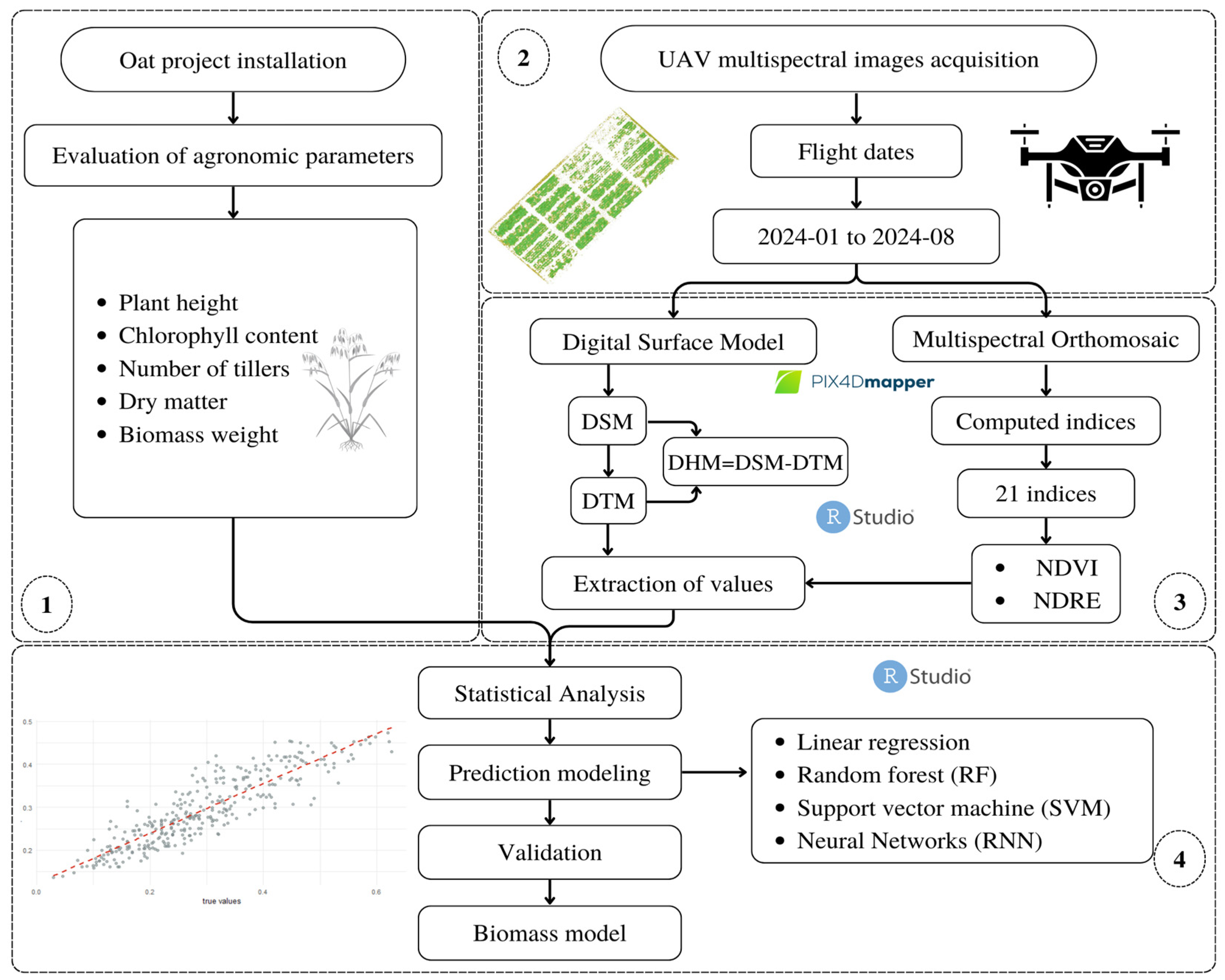
2.2. Methodological Framework

Figure 2 shows the comprehensive methodological framework used in this study, providing an overview of the sequential and integrative processes involved. The study is divided into several key stages: the first involves the collection of agronomic data, followed by the acquisition of information through UAV flights equipped with a multispectral camera. The third stage encompasses the extraction of spectral indices and photogrammetric processes, and finally, the training and validation of predictive models are conducted.

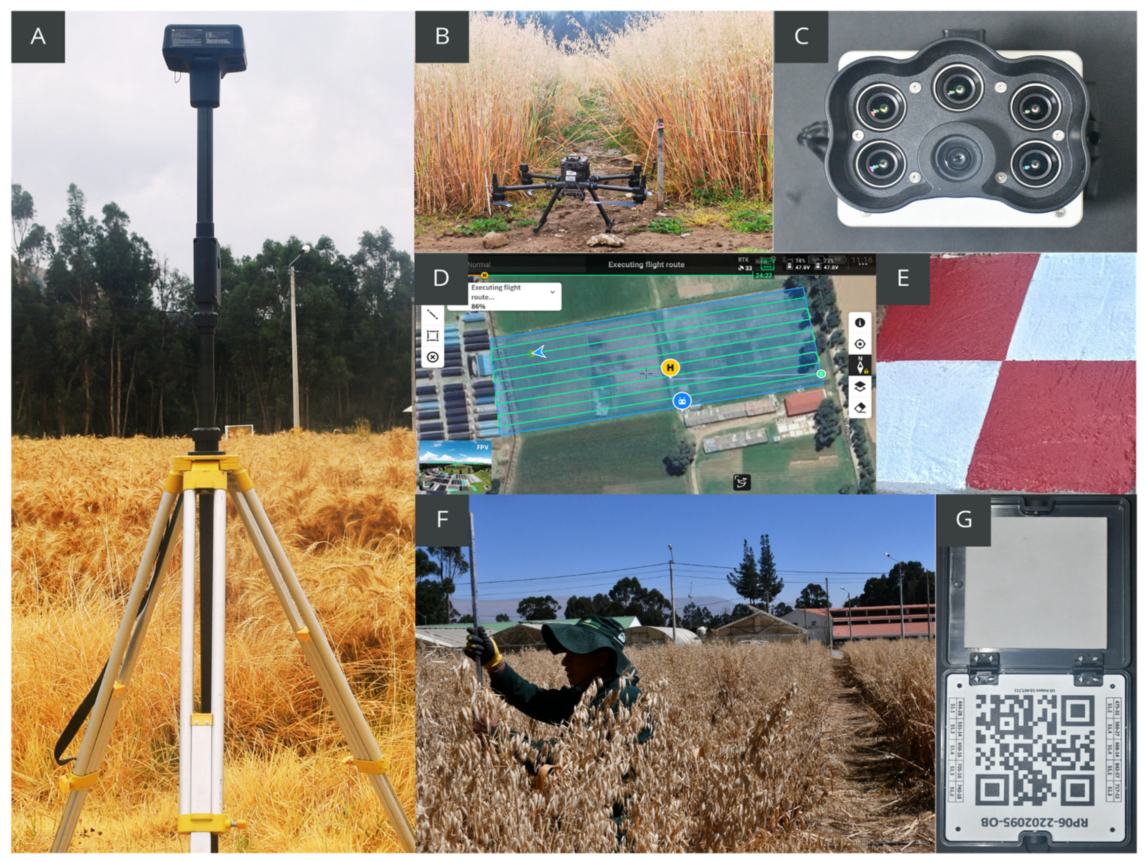
2.3. Image Acquisition and Preprocessing

The experiment was conducted using a multispectral camera MicaSense Red Edge P (Seattle, WA, USA) mounted on a DJI Matrice 300 RTK UAV (DJI Technology Co., Ltd., Shenzhen, China). The camera takes 16-bit multispectral digital images in five similar spectral bands—blue (475 ± 32 nm), green (560 ± 27 nm), red (668 ± 14 nm), NIR (842 ± 40 nm), and RE (717 ± 12 nm)—with a resolution of 1.6 megapixels ($1456 x 1088$ pixels); in addition, a GNSS receiver (D-RTK2 Mobile Station DJI, China) was used as a real-time kinematic (RTK) base station. Figure 3 shows the equipment used for capturing multispectral images in the evaluation plot.

The flight plan was executed around noon local time, at a height above ground of 150 m. Images were taken every 2.0 s with 75% front and side overlap. These digital images were stored in 16-bit .tiff format.

The process began with geolocating the images captured by the UAV equipped with a multispectral sensor, ensuring the accuracy of the geographic coordinates of the images. Six ground control points were used as fixed references on the terrain, allowing for correction of any deviation in the position of the images captured by the UAV. Once precise geolocation was established, individual images were aligned to form a coherent mosaic, a continuous and unified representation of the study area, where overlaps were removed and perspective differences were adjusted. Precise alignment is crucial to ensure that all geographic features are accurately represented in the mosaic.

Multispectral images were captured using the Micasense Red Edge P camera from an approximate height of 40 m, with an average of 14 flights conducted every 7 days. The UAV flight time was approximately 04 min and 15 s to cover the entire experimental field area.

During preprocessing, radiometric calibration and correction of the information were carried out. This step was essential to improve data quality by adjusting variations in lighting and atmospheric conditions that can affect the accuracy of measurements captured by the sensors. Radiometric calibration ensured that reflectance values in the images were consistent and comparable.

Photogrammetric processing was performed using Pix4D Pro Mapper v4.8.4. software (Prilly, Switzerland), geometrically corrected with field GCPs into the processing flow to enhance the topographic accuracy of the point cloud and the reflectance bands of the orthomosaic, with a final Ground Sampling Distance (GSD) of 2.8 cm. From the point cloud, a Digital Surface Model (DSM) was generated with the same resolution as the orthomosaic and exported in .tiff format.

Subsequently, a high-resolution orthomosaic was generated, geometrically corrected to maintain a uniform scale throughout its extent, eliminating distortions caused by perspective and topography. This allowed for precise measurements of distances, areas, and other features directly on the image.

Finally, spectral index maps were generated, such as the NDVI (Normalized Difference Vegetation Index), which are valuable tools for analyzing vegetation health and vigor. These indices were applied in various prediction algorithms, enabling informed decisions linked to precision agriculture.

2.4. Field Data Acquisition

The experimental work was carried out between December 2022 and July 2023. Twenty-four experimental plots measuring 16 m in length by 5 m in width were used, each subdivided into five rows. Six varieties of oats were selected based on their earliness and size, with four replications per variety. A total of 50 seeds were planted in each row, totaling 250 seeds per plot. Agronomic management followed conventional standards, including soil preparation with disc plowing and harrowing. Planting was carried out in rows, arranged in five rows per treatment, with 50 oat seeds planted in each row, spaced 30 cm apart.

Since planting coincided with the rainy season, additional irrigation was not necessary. Manual weeding was performed, and 150 kg of urea fertilizer was applied. Evaluations were conducted every thirty days throughout the experimental period. Additionally, six georeferenced concrete control points were installed in the surrounding area of the experimental plot.

In each plot, sampling points were marked every two meters along its length, specifically selecting the three central rows for evaluation. Biometric measurements of oat plants in the central rows were taken, with a total of 21 samples per plot. Plant height measurements were conducted from March to July 2023, using a 2 m aluminum ruler for data recording. Plant survival was assessed on four occasions in December 2022 and January and March 2023, applying the survival percentage formula [48].

$$\mathrm{\%} \mathrm{S}\mathrm{u}\mathrm{r}\mathrm{v}\mathrm{i}\mathrm{v}\mathrm{a}\mathrm{l}={\displaystyle \frac{(\mathrm{N}\mathrm{u}\mathrm{m}\mathrm{b}\mathrm{e}\mathrm{r} \mathrm{o}\mathrm{f} \mathrm{s}\mathrm{u}\mathrm{r}\mathrm{v}\mathrm{i}\mathrm{v}\mathrm{i}\mathrm{n}\mathrm{g} \mathrm{p}\mathrm{l}\mathrm{a}\mathrm{n}\mathrm{t}\mathrm{s})}{(\mathrm{N}\mathrm{u}\mathrm{m}\mathrm{b}\mathrm{e}\mathrm{r} \mathrm{o}\mathrm{f} \mathrm{p}\mathrm{l}\mathrm{a}\mathrm{n}\mathrm{t}\mathrm{s} \mathrm{p}\mathrm{l}\mathrm{a}\mathrm{n}\mathrm{t}\mathrm{e}\mathrm{d})}}\times 100$$

(1)

A flower count was conducted in March 2023. During the harvest on 25 July 2023, dry biomass was weighed using an analytical balance, and the number of tillers per plant was counted. In the post-harvest phase, seed weight was evaluated both per plant and per plot, proceeding with manual separation of straw from seeds and using a sorting machine for this purpose.

In the laboratory, two germination tests were conducted. The first test took place in April 2023 in an incubator at 25 °C, using four replicates of 100 seeds. Evaluations were conducted at 3, 7, and 10 days. The second test was conducted in July 2023 in a germination chamber at 25 °C under constant light and dark conditions, using trays with 72 holes filled with sterile peat. These evaluations were also conducted at 3, 7, and 10 days. Results were expressed as percentages of normal seedlings, abnormal seedlings, and hard, fresh, and dead seeds using the methodology described in [48].

$$\mathrm{\%} \mathrm{G}\mathrm{e}\mathrm{r}\mathrm{m}\mathrm{i}\mathrm{n}\mathrm{a}\mathrm{t}\mathrm{i}\mathrm{o}\mathrm{n}={\displaystyle \frac{(\mathrm{T}\mathrm{o}\mathrm{t}\mathrm{a}\mathrm{l} \mathrm{s}\mathrm{e}\mathrm{e}\mathrm{d}\mathrm{s} \mathrm{p}\mathrm{l}\mathrm{a}\mathrm{n}\mathrm{t}\mathrm{e}\mathrm{d})}{(\mathrm{T}\mathrm{o}\mathrm{t}\mathrm{a}\mathrm{l} \mathrm{s}\mathrm{e}\mathrm{e}\mathrm{d}\mathrm{s} \mathrm{g}\mathrm{e}\mathrm{r}\mathrm{m}\mathrm{i}\mathrm{n}\mathrm{a}\mathrm{t}\mathrm{e}\mathrm{d})}}\times 100$$

(2)

A total of six data collection sessions were conducted during the growing season, spanning from the early stem elongation stage to the late senescence stage. These field measurements were taken in December (14, 21) of 2022 and January 2023 (6,18), as well as on 22 February and 8 March 2023, on the same days as the studies and UAV flights conducted in December (14, 21, 28) of 2022, as well as January (6, 11, 18, 25), February (8, 10, 16, 22), and March (2, 8, 15) of 2023, totaling 14 flights to provide real-time ground data.

2.5. Extraction and Processing of Multispectral Images

For the processing and extraction of multispectral data, the photogrammetric process was initiated using Pix4D Pro Mapper software (Prilly, Switzerland). This software is essential for generating detailed orthomosaics from multiple images captured by the multispectral camera mounted on the UAV. This process included not only the generation of digital elevation models but also the fusion of spectral data to enhance the spatial and thematic resolution of the resulting images.

The R studio software (R Core Team) was used for the analysis and manipulation of the obtained geospatial data. Additionally, the Terra package for Hijmans [49] was employed for image processing and the extraction of spectral indices, and Quantum Geographical Information System software (QGIS 2.18.14, QGIS Development Team, Raleigh, NC, USA) was used for the vectorization of the images, enabling a more detailed analysis of the study plots.

For the extraction of indices, the derived spectral bands were used based on bibliographic equations from the Terra package [49]. With the indices calculated, a 30 cm buffer was created around the central point of each plant, and within this buffer, the zonal statistics of the maximum values of all pixels contained within the buffer were extracted.

To develop the benchmark models, we initially generated a set of 21 spectral indices. These indices included vegetation, soil, and water indices, and they are closely related to crop biomass. For each sampled point, a circular buffer with a radius of 0.25 m was used. The vegetation indices were calculated through different combinations of reflectance and compiled as predictors along with the pure spectral bands (

Table 1. Spectral indices derived from UAV-acquired multispectral images.

Indices	Equation	Description
Differenced Vegetation Index (DVI)	$Nir-Red$	[50]
Normalized Difference Vegetation Index (NDVI)	${\displaystyle \frac{Nir-Red}{Nir+Red}}$	[51]
Green Normalized Difference Vegetation (GNDVI)	${\displaystyle \frac{Nir-Green}{Nir+Green}}$	[52]
Normalized Difference Red Edge (NDRE)	${\displaystyle \frac{Nir-Re}{Nir+Re}}$	[52]
Enhanced Normalized Difference Vegetation Index (ENDVI)	${\displaystyle \frac{2\times Nir-Red-Blue}{2\times Nir+Red+Blue}}$	[53]
Renormalized Difference Vegetation Index (RDVI)	${\displaystyle \frac{Nir-Red}{\sqrt{Nir+Red}}}$	[54]
Enhanced Vegetation Index (EVI)	$G\times {\displaystyle \frac{(Nir-Red)}{(Nir+C1\times Red-C2\times Blue+L)}}$	[55]
Visible Difference Vegetation Index (VDVI)	${\displaystyle \frac{Nir-Red}{Nir+Red+Green}}$	[56]
Wide Dynamic Range Vegetation Index (WDRDVI)	${\displaystyle \frac{(Nir-Red)}{\sqrt{Nir+Red}}}$	[57]
Transformed Vegetation Index (TVI)	$0.5\times [120\times (Nir-Green\left)\right]$	[58]
Soil-Adjusted Vegetation index (SAVI)	${\displaystyle \frac{Nir-Red}{Nir+Red+L}}\times (1+L)$	[59]
Optimized Soil-Adjusted Vegetation Index (OSAVI)	${\displaystyle \frac{(Nir-Red)}{Nir+Red+0.16}}$	[59]
Content Validity Index (CVI)	$Nir\times \left({\displaystyle \frac{Red}{Green}}\right)$	[60]
Modified Soil Adjusted Vegetation Index (MSAVI)	${\displaystyle \frac{2\times Nir+1 \sqrt{{(2 x Nir+1)}^2-8\times (Nir-Red)}}{2}}$	[61]
Modified Chlorophyll Absorption in Reflectance Index (MCARI)	${\displaystyle \frac{\left(Red-Green\right)-2\times (Red-Blue)}{\frac{Red}{Green}}}$	[62]
Transformed Chlorophyll Absorption in the Reflectance Index (TCARI)	$3\times ((Red-Green)-0.2\times (Red-Blue)\times ({\displaystyle \frac{Red}{Green}}))$	[63]
Normalized Pigment Chlorophyll Reflectance (NPCI)	${\displaystyle \frac{Red-Blue}{Red+Blue}}$	[60,64]
Green Coverage Index (GCI)	${\displaystyle \frac{Nir}{Green}}-1$	[56]
Red-Edge Chlorophyll Index (RECI)	${\displaystyle \frac{Nir}{Re}}-1$	[65]
Structure Insensitive Pigment Index (SIPI)	${\displaystyle \frac{Nir-Blue}{Nir-Red}}$	[66]
Anthocyanin Reflectance Index (ARI)	${\displaystyle \frac{1}{Green}}-{\displaystyle \frac{1}{Red}}$	[67]

Multispectral imagery central wavelengths: Blue, Green, Red, Red edge (Re), and Nir: 474, 560, 668, 717, and 840 nm.

).

The selection of these indices was not random. Each index was chosen based on its theoretical and empirical capacity to reflect key aspects of crop condition and health, such as biomass, soil coverage, and plant water content, which are critical for accurate yield estimation.

We initially calculated a broad range of indices to ensure that we covered all potential variables that could influence oat yield. Subsequently, we applied statistical techniques to select the two most significant indices, which provided valuable information for the predictive models.

2.6. Data Analysis and Selection of Predictor Variables

For the analysis of agronomic data, homoscedasticity tests and normality tests [68] were conducted to determine the distribution and symmetry of the data. Additionally, boxplots were constructed to identify outliers, enabling efficient data cleaning and refinement.

Spectral indices were extracted for each flight date, totaling 28 flights for oat crop monitoring. Twenty-one spectral indices were evaluated in each flight. Subsequently, a correlation matrix was generated between agronomic variables and spectral indices derived from multispectral images, considering flight dates and days elapsed since planting, ranging from 20 to 250 days. Out of the 21 indices evaluated, only 2 exhibited suitable behavior or correlation for further processing: NDVI and NDRE.

Furthermore, a significance matrix was developed to identify indices showing higher Pearson’s correlation with agronomic variables. It was observed that data obtained beyond 100 days post-planting exhibited stronger correlations with agronomic variables measured in the field. The process included correlating variables derived from spectral indices with agronomic parameters measured using traditional techniques such as height, germination percentage, flower count, grain dry matter, stem count, survival percentage, and dry biomass weight. This correlation was crucial for identifying significant relationships and understanding complex patterns affecting biomass estimation.

Using this information, Principal Component Analysis (PCA) was performed considering only days post-planting exceeding 100. Subsequently, a detailed correlation analysis was conducted to identify spectral indices most strongly related to agronomic variables. This approach helped identify critical periods and the most relevant spectral indices. These tools enabled clustering of areas with similar characteristics and reduced data dimensionality, facilitating identification of the most relevant variables.

Identification of key variables for the study was accomplished through a Pearson correlation matrix. This matrix identified variables significantly correlated with the variable of interest, namely dry biomass weight and the most representative flight days.

2.6.1. Modeling and Estimation Algorithms

We use four predictive regression algorithms. First, linear regression models the relationship between independent variables and a dependent variable through a straight line, which is useful for predicting numerical value [69,70,71]. Second, Random Forest combines multiple decision trees to improve prediction accuracy and reduce overfitting [72,73,74].

Third, Neural Networks (NNs) are brain-inspired models composed of layers of interconnected nodes that process information and learn complex patterns through feedback [75]. These models are suitable for deep learning and complex pattern recognition problems [76,77].

Finally, Support Vector Machines (SVMs) are supervised learning algorithms that seek the optimal hyperplane to separate data into different classes in a high-dimensional space [78]. They are effective on both small and large datasets and can be applied to linear and nonlinear classification problems. Although they may face computational challenges with very large datasets, optimization techniques and advanced computational resources can enhance their efficiency [79,80].

2.6.2. Model Tuning and Evaluation

The response variable was selected as a vector, while the predictor variables were grouped into a matrix, with the data split into 70% for training and 30% for testing. The split was performed randomly and not based on different time periods.

To optimize the performance of the machine learning models, it is essential to fine-tune their hyperparameters. We used the training samples to calibrate the models using the Grid Search method [81,82] which exhaustively evaluates all possible combinations of hyperparameters. Ten-fold cross-validation and the coefficient of determination (R²) were employed as evaluation metrics to ensure the robustness of the models [83,84].

For Random Forest, the hyperparameters ‘ntree’ (testing values between 20 and 180) and ‘mtry’ (testing values between 2 and 14) were adjusted, with other parameters kept at their default settings. For the Support Vector Machine (SVM), ‘C’ (testing values between 0.01 and 10) and ‘Gamma’ (testing values between 0.1 and 1) were adjusted, while the remaining parameters were also set to their default values.

The architecture of the neural network used has two hidden layers with 6 and 5 neurons, respectively, with an input layer with the number of nodes equal to the number of predictive variables and the output layer with one neuron and a linear continuous response.

The modeling was carried out in R, using the ‘randomForest’, ‘e1071’ and neuralnet libraries [85].

3. Results

3.1. Descriptive Statistics of Agronomic Variables

Multiple metrics reflecting oat crop development were evaluated. Various descriptive statistics were analyzed (

Table 2. Descriptive agronomic statistics of oat variables.

Agronomic Variable	Prom	Mean	Min	Max	σ
Height (meters) (h)	1.50	1.50	1.13	1.88	0.15
Tillers (t)	29.97	29.00	5.00	61.00	11.57
Dry matter (kg) (dm)	0.29	0.28	0.03	0.63	0.12
Grain weight (kg) (gw)	0.04	0.04	0.00	0.10	0.02
Flowers (f)	14.76	16.00	3.00	26.00	5.38
Germination percentage (gp)	0.72	0.79	0.30	0.88	0.18
Germination in emergency chamber (gem)	0.62	0.71	0.15	0.78	0.18
Total plants (tp)	31.87	33.00	15.00	40.00	5.47
Survival rate (sr)	0.64	0.66	0.30	0.80	0.11
Germination rate (gr)	10.27	11.29	4.29	12.57	2.55

) for the parameters of each evaluated variable.

The oat at harvest reached an average height of 1.50 m, with a standard deviation of 0.15 m, and a range varying between 1.13 and 1.88 m. The number of stems per plant had a mean of 29.97, with a standard deviation of 11.57, ranging from 5 to 61 stems. Regarding dry matter, plants averaged 0.29 kg, with a standard deviation of 0.12 kg and a range from 0.03 to 0.63 kg. Grain yield per plant averaged 0.04 kg, with a standard deviation of 0.02 kg and a range from 0.00 to 0.10 kg. Additionally, an average of 14.76 flowers per plant was observed, with a standard deviation of 5.38, and a range fluctuating between 3 and 26 flowers. Germination data showed an average percentage of 72%, with a standard deviation of 18% and a range from 30% to 88%.

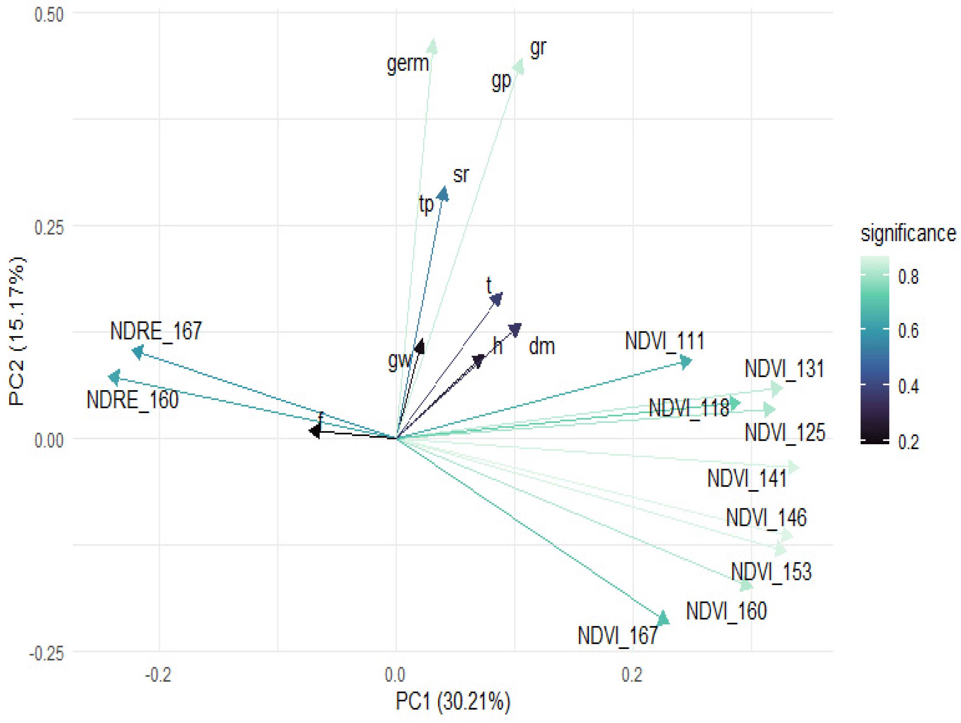
3.2. Spectral Variable Analysis

3.2.1. Significance Correlation Matrix

The correlation matrix (Figure 4) displays Pearson correlation coefficients between agronomic variables and filtered spectral indices, calculated using the Corrplot library for Wei T [86], reflecting their linear relationships. Matrix values range from −1 to 1, where 1 indicates a perfect positive correlation, −1 is a perfect negative correlation, and 0 is no correlation. The main diagonal of the matrix always holds 1, as each variable correlates perfectly with itself.

This analysis was crucial for identifying patterns, detecting multicollinearity, and selecting the most relevant variables concerning dry biomass weight (bw), without seeds. In the correlation analysis with dry matter (dm) as the variable of interest, varying levels of association with several variables were found.

The correlation coefficient between dry matter (dm) and NDRE_160 was −0.1, indicating a weak negative correlation. NDVI, measured on days 111, 131, 141, and 146, showed correlation values ranging from 0.15 to 0.21 with dry matter, suggesting a weak to moderate positive correlation. Similarly, agronomic variables exhibited a positive correlation of 0.2 with dry matter (dm). In contrast, the number of stems displayed a strong positive correlation of 0.76 with dry matter, suggesting that a higher number of stems is strongly associated with an increase in dry matter. Additionally, the grain weight showed a positive correlation of 0.2 with dry matter. The flight days that showed the highest correlation were 111, 118, 125, 131, 141, 146, 153, 160, and 167.

3.2.2. Principal Component Analysis

Principal Component Analysis (PCA) enabled a reduction in data dimensionality by eliminating redundancies and focusing the analysis on the most influential variables. This reduction not only simplified the complexity of the dataset but also decreased both squared and absolute errors in the predictive models, thereby enhancing their accuracy and efficiency. Consequently, PCA has established itself as a key tool for optimizing the performance of machine learning algorithms in biomass estimation and crop yield prediction [87,88,89,90].

Figure 5 shows PCA, where Principal Component 1 (PC1) explains 30.21% of the variance and Principal Component 2 (PC2) explains 15.17%. Each arrow represents an original variable projected onto the principal component space; the direction and length of the arrows indicate how these variables contribute to the components.

Variables NDRE_167 and NDRE_160 are negatively correlated with PC1, whereas NDVI variables (111, 118, 125, 131, 141, 146, 153, 160, 167) contribute significantly and positively to PC1. Other variables such as germ, gp, gr, sr, tp, t, gw, hr, and dm contribute to PC2 to varying degrees. The color of the arrows reflects their significance level, with darker colors indicating greater significance.

In particular, the dry matter variable “dm” projects primarily in the positive direction of PC2 and slightly in the negative direction of PC1, suggesting a positive correlation with Principal Component 2 and a slight negative correlation with Principal Component 1. The darker intensity of the “dm” arrow indicates moderate to high significance.

PCA reveals that NDVI variables strongly influence PC1, while other variables like germ and gp contribute more significantly to PC2. The variable “dm” stands out for its influence on PC2, correlating positively with other variables that also contribute to this component.

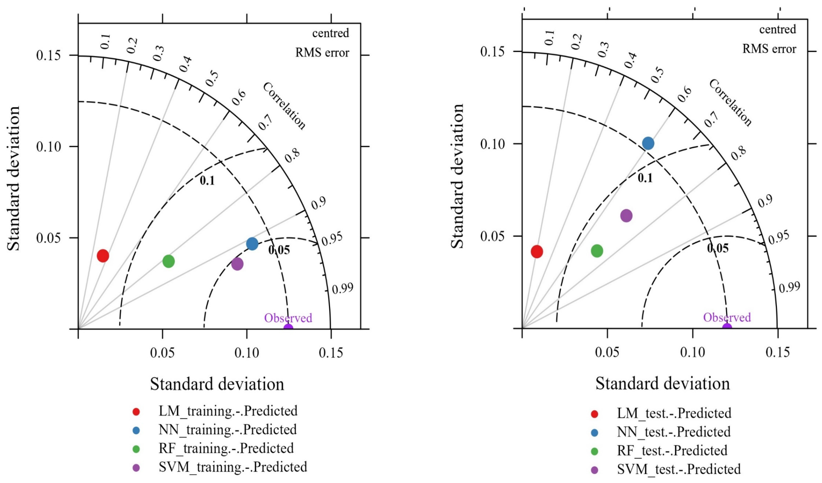
3.3. Model Performance

Figure 6 shows two Taylor diagrams illustrating the performance of the models used to estimate dry matter: linear regression, Neural Network, Random Forest, and Support Vector Machine. Each point on the graph represents the accuracy of these models in terms of standard deviation, correlation coefficient, and root mean square error (RMSE) for both the training and test datasets. In the test set, the Support Vector Machine shows strong performance with a correlation coefficient (r) of 0.93, followed by the Neural Network model with an r of 0.91, indicating high precision in predicting dry matter (dm).

The Random Forest and Support Vector Machine models show outstanding fit in the training set with r values of 0.70 and 0.72, respectively, demonstrating high learning capacity. However, their performance in the test set is more modest. Overall, the Support Vector Machine model exhibits the best overall performance, combining excellent fit in the training set with solid performance in the test set. On the other hand, the linear regression model has the lowest correlation coefficient values in both the test and training sets, highlighting its lower effectiveness compared to the other evaluated models.

The Support Vector Machine shows the best overall performance as it demonstrates low RMSE in both datasets and high r values. Additionally, the Random Forest model also performs well in the test set, although not as strongly as the SVM. The Neural Network model shows good fit in training but lower performance in testing, suggesting overfitting. The linear regression model performs the poorest, with the highest RMSE values and the lowest r values.

3.4. Predictor Estimation

In the results table of the linear regression (

Table 3. Characteristics and estimation of predictors.

Linear Regression
Residual		Coefficient
Min	−0.208		Intercept	NDVI 111	NDVI 125	NDVI 131	h
1Q	−0.091	Estimate	−0.439	0.541	−1.148	1.256	0.184
Median	−0.016	Std	0.188	0.256	0.457	0.363	0.045
3Q	0.075	Error	−2.336	2.123	−2.513	3.464	4.075
Max	0.314	t-values	0.02	0.034	0.012	0.004	5.8
Parameters	RF		SVM		NN
Hyperparameters	Node size	100	Cost	1	* HL 2	Neurons 5
	Trees	500	γ	0.1		Neurons 3
	N° var	4	ε	0.01
Residual	Mean of squared	0.011	N° of vectors	294
	% var	52.23	SVM	Radial

* 5% confidence Interval; RF (Random Forest), SVM (Support Vector Machine), NN (Neural Network); HL = hidden layer; 70% training set and 30% test set.

), coefficient estimates for various predictors used in the model are presented. The intercept has a value of −0.439 (p = 0.020104), which is significant and suggests that, in the absence of other factors, forage biomass would have a negative value. The coefficient for NDVI_111 is 0.541 (p = 0.034539), indicating a positive and significant relationship with biomass. On the other hand, NDVI_125 has a coefficient of −1.148 (p = 0.012474), showing a significant negative relationship. NDVI_131 has a coefficient of 1.256 (p = 0.000604), indicating a positive and highly significant relationship. Finally, plant height (h) has a coefficient of 0.184 (p = 5.805), also significant, implying that an increase in height is associated with an increase in forage biomass.

The hyperparameters and metrics of predictive models provide crucial information about their configuration and performance. In the Random Forest model, a node size of 100 indicates that each terminal node must have at least 100 observations, with 500 trees improving accuracy but increasing server processing time, and four variables considered for splitting each node. For the Support Vector Machine model, the cost parameter is set to one, balancing between a wide margin and correct classification of training points; gamma of 0.1 indicates that only nearby points influence the decision boundary; epsilon of 0.01 reflects high precision, and 294 support vectors are used. In the Neural Network model, two hidden layers are configured with five and three neurons, respectively, affecting its ability to capture complex patterns.

Regarding residual performance metrics, the mean squared residual is 0.011 for the Random Forest model, suggesting good accuracy, and the percentage of explained variance is 52.23%, indicating that this percentage of variability in the data is explained by the predictors used in the model, but also showing that 47.77% of the variability remains unexplained. The performance of different models shows variability in predictive capability. For linear regression, the coefficient of determination (R²) is 0.12 in the training set and 0.04 in the test set, indicating low explanatory power.

Table 4. Performance of predictive models.

	Linear Regression		RF		SVM		NN
Training	R2	0.12	R2	0.68	R2	0.87	R2	0.83
	RMSE	0.117	RMSE	0.080	RMSE	0.047	RMSE	0.051
	MAE	0.096	MAE	0.063	MAE	0.030	MAE	0.040
Test	R2	0.04	R2	0.52	R2	0.50	R2	0.35
	RMSE	0.119	RMSE	0.087	RMSE	0.085	RMSE	0.110
	MAE	0.097	MAE	0.069	MAE	0.066	MAE	0.086

5% confidence Interval; RF (Random Forest), SVM (Support Vector Machine), NN (Neural Network).

shows the performance of four models used (linear regression, Random Forest, Support Vector Machine, and Neural Networks) for estimating dry matter in the training and test datasets, evaluated using the metrics R², RMSE, and MAE. Random Forest and Support Vector Machine stand out with superior results: in training, RF achieves an R² of 0.68 with an RMSE of 0.080 and an MAE of 0.063, while SVM achieves an R² of 0.87 with an RMSE of 0.047 and an MAE of 0.030. In testing, RF obtains an R² of 0.68 with an RMSE of 0.080 and an MAE of 0.063, and SVM reaches an R² of 0.83 with an RMSE of 0.051 and an MAE of 0.040, demonstrating robust generalization performance.

On the other hand, Neural Networks show better performance in training with an R² of 0.83, but significantly decrease in testing with an R² of 0.35, indicating potential overfitting during training. In contrast, linear regression shows the lowest performance with an R² of 0.12 and 0.04, an RMSE of 0.117 and 0.119, and an MAE of 0.096 and 0.097 in training and testing, respectively. The Support Vector Machine demonstrates consistent performance in both training and testing, with an R² of 0.87 and 0.50, respectively, along with low RMSE and MAE values.

The Support Vector Machine proves to be the most effective model for this dataset, while linear regression exhibits more limited performance in comparison.

3.5. Predictive Model for Biomass Estimation

Figure 7 depicts the estimation of dry matter in forage oats using the evaluated models: LM (Linear Model), NN (Neural Network), RF (Random Forest), and SVM (Support Vector Machine). Each map displays the estimation in 0.25 m² grid cells, colored according to their weight in kilograms, allowing for observation of the variation in predictions from each model.

LM predominantly predicts medium weights (0.10 kg to 0.30 kg), with few cells at extreme values. NN shows greater variability, with cells ranging from 0.05 kg to 0.55 kg, highlighting areas with higher biomass. RF exhibits a trend similar to LM, with average values around 0.29 kg. In contrast, SVM shows a more balanced but conservative distribution, predominantly with lower weights (0.05 kg to 0.25 kg). Areas with gray outlines in all maps indicate regions with an estimated dry matter of zero due to the absence of vegetation.

These maps allow for comparing the predicted biomass distribution by each model, facilitating understanding of their differences. In summary, SVM is the model that most closely approximates the average dry matter evaluated in the field, with an estimation ranging between 0.05 kg and 0.25 kg, demonstrating its effectiveness in estimating dry matter in forage oats.

4. Discussion

The use of UAVs for biomass estimation has proven to be an efficient and accurate method, as indicated by a coefficient of determination (R²) of 0.52. Although this value is lower than those reported in previous studies, such as that by Lussem [91], who recorded R² values between 0.56 and 0.73, it is important to note that the RMSE values in his study were considerably higher, ranging from 0.274 to 0.416. On the other hand, studies like Coelho’s [92], report significantly higher R² values (0.70–0.89), which better capture data variability, albeit with higher absolute errors (RMSE from 370 to 1825 kg ha⁻¹). In contrast, the present study reports an RMSE of 0.080 and MAE of 0.063, suggesting that while a model with a higher R² may better explain variance, the higher absolute and squared errors could reduce its reliability due to sensitivity to deviations or outliers [93,94,95]. Therefore, balancing explanatory power and accuracy is crucial in the selection of estimation models. Despite these differences, the UAV approach continues to provide suitable and often superior estimates in many contexts [96,97].

Estimating biomass in crops through remote sensing involves several critical and interconnected objectives aimed at improving model accuracy and applicability. One of the primary goals is to identify the variables that correlate with reference biomass obtained in the field, which requires careful selection and evaluation of different sensors and remote sensing techniques [98]. Equally important is the development of accurate and scalable models that incorporate both parametric and non-parametric algorithms, and the integration of data from multiple sensors to enhance estimation precision [91]. However, it is crucial to recognize that the accuracy of these estimates can be affected by various sources of uncertainty. Environmental factors, such as light conditions, wind, and humidity, can significantly influence UAV image capture, highlighting the need for detailed analyses to identify and mitigate these potential errors [99]. Additionally, the spatial and temporal scale of the data plays a vital role, as different resolutions can significantly impact the accuracy of biomass models, necessitating constant methodological adjustments [98]. While the progress made is promising, applying these models on a larger scale presents additional challenges [100]. The transferability of these models across diverse geographic and temporal conditions must be rigorously evaluated to ensure their robustness and accuracy in large-scale applications [91,97,101]. In this context, it is essential to consider how environmental variability might affect the applicability of the results in different regions and under varying climatic conditions.

Finally, to advance toward more efficient and precise methodologies in global agricultural management, it is crucial not only to enhance the accuracy of existing models but also to address the identified limitations, such as environmental factors and model scalability, in future research. Emphasizing the importance of a critical and thorough evaluation of the results ensures that the proposed solutions are viable and effective in a broader agricultural context.

The use of machine learning models such as regression, Random Forest, Support Vector Machines, and Neural Networks for biomass estimation using UAVs has been extensively researched. Regression is useful for handling highly correlated predictors and has been effective in predicting biomass in various vegetation types, notably reducing dimensionality and improving estimation accuracy [102]. RF is robust and accurate, successfully used in estimating biomass in different forests and crops, including forage oats, due to its ability to handle datasets with many features without overfitting [5,103]. The Support Vector Machine, capable of handling nonlinear and high-dimensional data, has also proven effective in biomass prediction using complex spectral data, although proper parameter selection can be challenging [104]. Neural Networks, on the other hand, can model complex nonlinear relationships and have been used in numerous studies to predict biomass, providing a significant advantage by combining multiple spectral and temporal variables, as seen in Bazzo [33]. The literature and current research suggest that combining spectral data with machine learning algorithms can significantly enhance biomass estimation accuracy, with each model offering specific advantages that can be exploited to improve estimation precision and robustness, serving as valuable tools for crop management and monitoring [73].

When applying different modeling approaches for biomass estimation via UAVs, it has been observed that each technique has its own strengths and limitations. For instance, linear regression is straightforward and easily interpretable but may fail to capture complex nonlinear relationships between input variables and biomass. Random Forest, which constructs multiple decision trees and averages their results, has proven robust and accurate but can be prone to overfitting with noisy datasets [32,91]. Support Vector Machines are effective in high-dimensional problems with small samples, although selecting appropriate parameters can be challenging.

Artificial Neural Networks are powerful for modeling complex nonlinear relationships and have shown high accuracy in biomass estimation, though their interpretability and tendency to become stuck in local minima can be significant disadvantages [33]. These findings are consistent with other research utilizing UAVs for biomass estimation across different pasture types and vegetation [5], emphasizing the importance of selecting the appropriate model based on dataset characteristics and study objectives.

5. Conclusions

The germination index showed low correlations with the target variable, rendering it insignificant for the predictive model. Statistical analyses revealed it is more closely associated with other variables not directly linked to the target variable. In contrast, dry matter is strongly correlated with NDVI values and plant height, indicating that these variables are more predictive. NDVI values, reflecting vegetation health along with dry matter and height, serve as better indicators of crop status and performance. Therefore, focusing on these variables enhances predictive model accuracy.

Using UAVs to estimate forage biomass is a powerful tool that offers high resolution and flexibility in agricultural monitoring. However, to maximize its benefits, logistical, technical, and validation challenges must be overcome, alongside considerations of environmental conditions. With proper implementation, UAVs have the potential to revolutionize crop management practices and provide valuable data for agricultural decision-making.

The analysis of predictive models, including Random Forest, Support Vector Machines, and Neural Networks, has revealed significant variations in terms of accuracy and performance. The presentation of these results has been complemented by an explanation of the hyperparameters and the incorporation of visualizations, with the aim of providing a clearer and more practical perspective. This approach not only highlights the effectiveness of the models but also facilitates the interpretation and application of the results in real-world contexts, contributing to a more effective integration into agricultural decision-making. Consequently, an approach has been adopted that strives to make the models more accessible and useful.

References

1. Gupta, A.K.; Sharma, M.L.; Khan, M.A.; Pandey, P.K. Promotion of improved forage crop production technologies: Constraints and strategies with special reference to climate change. In Molecular Interventions for Developing Climate-Smart Crops: A Forage Perspective; Springer: Singapore, 2023; pp. 229–236. [Google Scholar] [CrossRef]
2. Trevisan, L.R.; Brichi, L.; Gomes, T.M.; Rossi, F. Estimating Black Oat Biomass Using Digital Surface Models and a Vegetation Index Derived from RGB-Based Aerial Images. Remote Sens. 2023, 15, 1363. [Google Scholar] [CrossRef]
3. Garland, G. Sustainable management of agricultural soils: Balancing multiple perspectives and tradeoffs. In EGU General Assembly Conference Abstracts; EGU: Vienna, Austria, 2023. [Google Scholar] [CrossRef]
4. Francaviglia, R.; Almagro, M.; Vicente-Vicente, J.L. Conservation Agriculture and Soil Organic Carbon: Principles, Processes, Practices and Policy Options. Soil Syst. 2023, 7, 17. [Google Scholar] [CrossRef]
5. Sharma, P.; Leigh, L.; Chang, J.; Maimaitijiang, M.; Caffé, M. Above-Ground Biomass Estimation in Oats Using UAV Remote Sensing and Machine Learning. Sensors 2022, 22, 601. [Google Scholar] [CrossRef] [PubMed]
6. Fodder, K.; Jimenez-Ballesta, R.; Srinivas Reddy, K.; Samuel, J.; Kumar Pankaj, P.; Gopala Krishna Reddy, A.; Rohit, J.; Reddy, K.S. Fodder Grass Strips for Soil Conservation and Soil Health. Chem. Proc. 2022, 10, 58. [Google Scholar] [CrossRef]
7. Katoch, R. Nutritional Quality of Important Forages. In Techniques in Forage Quality Analysis; Springer: Singapore, 2023; pp. 173–185. [Google Scholar] [CrossRef]
8. Barrett, B.A.; Faville, M.J.; Nichols, S.N.; Simpson, W.R.; Bryan, G.T.; Conner, A.J. Breaking through the feed barrier: Options for improving forage genetics. Anim. Prod. Sci. 2015, 55, 883–892. [Google Scholar] [CrossRef]
9. Kim, K.S.; Tinker, N.A.; Newell, M.A. Improvement of Oat as a Winter Forage Crop in the Southern United States. Crop Sci. 2014, 54, 1336–1346. [Google Scholar] [CrossRef]
10. McCartney, D.; Fraser, J.; Ohama, A. Annual cool season crops for grazing by beef cattle. A Canadian Review. Can. J. Anim. Sci. 2011, 88, 517–533. [Google Scholar] [CrossRef]
11. Kumar, S.; Vk, S.; Sanjay, K.; Priyanka; Gaurav, S.; Jyoti, K.; Kaushal, R. Identification of stable oat wild relatives among Avena species for seed and forage yield components using joint regression analysis. Ann. Plant Soil Res. 2022, 24, 601–605. [Google Scholar] [CrossRef]
12. Espinoza-Montes, F.; Nuñez-Rojas, W.; Ortiz-Guizado, I.; Choque-Quispe, D. Forage production and interspecific competition of oats (Avena sativa) and common vetch (Vicia sativa) association under dry land and high-altitude conditions. Rev. De. Investig. Vet. Del. Peru. 2018, 29, 1237–1248. [Google Scholar] [CrossRef]
13. INEI. Sistema Estadistico Nacional-Provincia de Lima 2018, 1–508. Available online: https://www.inei.gob.pe/media/MenuRecursivo/publicaciones_digitales/Est/Lib1583/15ATOMO_01.pdf (accessed on 4 September 2024).
14. Aníbal, C.; Mayer, F. Producción de Carne y Leche Bovina en Sistemas Silvopastoriles; Instituto Nacional de Tecnología Agropecuaria: Buenos Aires, Argentina, 2017. [Google Scholar]
15. Santacoloma-Varón, L.E.; Granados-Moreno, J.E.; Aguirre-Forero, S.E. Evaluación de variables agronómicas, calidad del forraje y contenido de taninos condensados de la leguminosa Lotus corniculatus en respuesta a biofertilizante y fertilización química en condiciones agroecológicas de trópico alto andino colombiano. Entramado 2017, 13, 222–233. [Google Scholar] [CrossRef]
16. Mariana, M.P. Determinación de Variables Agronómicas del Cultivo de Maíz Mediante Imágenes Obtenidas Desde un Vehículo Aéreo no Tripulado (VANT). Thesis Instituto Mexicano de Tecnología del Agua, Jiutepec, Mexico, 2017. Available online: http://repositorio.imta.mx/handle/20.500.12013/1750 (accessed on 4 September 2024).
17. Watanabe, K.; Guo, W.; Arai, K.; Takanashi, H.; Kajiya-Kanegae, H.; Kobayashi, M.; Yano, K.; Tokunaga, T.; Fujiwara, T.; Tsutsumi, N.; et al. High-throughput phenotyping of sorghum plant height using an unmanned aerial vehicle and its application to genomic prediction modeling. Front. Plant Sci. 2017, 8, 254051. [Google Scholar] [CrossRef] [PubMed]
18. Matsuura, Y.; Heming, Z.; Nakao, K.; Qiong, C.; Firmansyah, I.; Kawai, S.; Yamaguchi, Y.; Maruyama, T.; Hayashi, H.; Nobuhara, H. High-precision plant height measurement by drone with RTK-GNSS and single camera for real-time processing. Sci. Rep. 2023, 13, 6329. [Google Scholar] [CrossRef]
19. Ji, Y.; Chen, Z.; Cheng, Q.; Liu, R.; Li, M.; Yan, X.; Li, G.; Wang, D.; Fu, L.; Ma, Y.; et al. Estimation of plant height and yield based on UAV imagery in faba bean (Vicia faba L.). Plant Methods 2022, 18, 26. [Google Scholar] [CrossRef]
20. Ibiev, G.Z.; Savoskina, O.A.; Chebanenko, S.I.; Beloshapkina, O.O.; Zavertkin, I.A. Unmanned Aerial Vehicles (UAVs)-One of the Digitalization and Effective Development Segments of Agricultural Production in Modern Conditions. In AIP Conference Proceedings; AIP Publishing: Melville, NY, USA, 2022; Volume 2661. [Google Scholar] [CrossRef]
21. Hütt, C.; Bolten, A.; Hüging, H.; Bareth, G. UAV LiDAR Metrics for Monitoring Crop Height, Biomass and Nitrogen Uptake: A Case Study on a Winter Wheat Field Trial. PFG-J. Photogramm. Remote Sens. Geoinf. Sci. 2023, 91, 65–76. [Google Scholar] [CrossRef]
22. Plaza, J.; Criado, M.; Sánchez, N.; Pérez-Sánchez, R.; Palacios, C.; Charfolé, F. UAV Multispectral Imaging Potential to Monitor and Predict Agronomic Characteristics of Different Forage Associations. Agronomy 2021, 11, 1697. [Google Scholar] [CrossRef]
23. Radoglou-Grammatikis, P.; Sarigiannidis, P.; Lagkas, T.; Moscholios, I. A compilation of UAV applications for precision agriculture. Comput. Netw. 2020, 172, 107148. [Google Scholar] [CrossRef]
24. Lottes, P.; Khanna, R.; Pfeifer, J.; Siegwart, R.; Stachniss, C. UAV-Based Crop and Weed Classification for Smart Farming. In Proceedings of the 2017 IEEE International Conference on Robotics and Automation (ICRA), Singapore, 29 May–3 June 2017. [Google Scholar]
25. Munghemezulu, C.; Mashaba-Munghemezulu, Z.; Ratshiedana, P.E.; Economon, E.; Chirima, G.; Sibanda, S. Unmanned Aerial Vehicle (UAV) and Spectral Datasets in South Africa for Precision Agriculture. Data 2023, 8, 98. [Google Scholar] [CrossRef]
26. Gitelson, A.A.; Vina, A.; Arkebauer, T.J.; Rundquist, D.C.; Keydan, G.; Leavitt, B. Remote estimation of leaf area index and green leaf biomass in maize canopies. Geophys. Res. Lett. 2003, 30, 1248. [Google Scholar] [CrossRef]
27. Belton, D.; Helmholz, P.; Long, J.; Zerihun, A. Crop Height Monitoring Using a Consumer-Grade Camera and UAV Technology. PFG-J. Photogramm. Remote Sens. Geoinf. Sci. 2019, 87, 249–262. [Google Scholar] [CrossRef]
28. Hassan, M.A.; Yang, M.; Fu, L.; Rasheed, A.; Zheng, B.; Xia, X.; Xiao, Y.; He, Z. Accuracy assessment of plant height using an unmanned aerial vehicle for quantitative genomic analysis in bread wheat. Plant Methods 2019, 15, 37. [Google Scholar] [CrossRef]
29. Schreiber, L.V.; Atkinson Amorim, J.G.; Guimarães, L.; Motta Matos, D.; Maciel da Costa, C.; Parraga, A. Above-ground Biomass Wheat Estimation: Deep Learning with UAV-based RGB Images. Appl. Artif. Intell. 2022, 36. [Google Scholar] [CrossRef]
30. Bendig, J.; Bolten, A.; Bennertz, S.; Broscheit, J.; Eichfuss, S.; Bareth, G. Estimating Biomass of Barley Using Crop Surface Models (CSMs) Derived from UAV-Based RGB Imaging. Remote Sens. 2014, 6, 10395–10412. [Google Scholar] [CrossRef]
31. Jin, Y.; Yang, X.; Qiu, J.; Li, J.; Gao, T.; Wu, Q.; Zhao, F.; Ma, H.; Yu, H.; Xu, B. Remote Sensing-Based Biomass Estimation and Its Spatio-Temporal Variations in Temperate Grassland, Northern China. Remote Sens. 2014, 6, 1496–1513. [Google Scholar] [CrossRef]
32. Zhang, H.; Sun, Y.; Chang, L.; Qin, Y.; Chen, J.; Qin, Y.; Chen, J.; Qin, Y.; Du, J.; Yi, S.; et al. Estimation of Grassland Canopy Height and Aboveground Biomass at the Quadrat Scale Using Unmanned Aerial Vehicle. Remote Sens. 2018, 10, 851. [Google Scholar] [CrossRef]
33. Bazzo, C.O.G.; Kamali, B.; Hütt, C.; Bareth, G.; Gaiser, T. A Review of Estimation Methods for Aboveground Biomass in Grasslands Using, U.A.V. Remote Sens. 2023, 15, 639. [Google Scholar] [CrossRef]
34. Kurbanov, R.; Panarina, V.; Polukhin, A.; Lobachevsky, Y.; Zakharova, N.; Litvinov, M.; Rebouh, N.Y.; Kucher, D.E.; Gureeva, E.; Golovina, E.; et al. Evaluation of Field Germination of Soybean Breeding Crops Using Multispectral Data from UAV. Agronomy 2023, 13, 1348. [Google Scholar] [CrossRef]
35. Chen, R.; Chu, T.; Landivar, J.A.; Yang, C.; Maeda, M.M. Monitoring cotton (Gossypium hirsutum L.) germination using ultrahigh-resolution UAS images. Precis. Agric. 2018, 19, 161–177. [Google Scholar] [CrossRef]
36. Zhang, Y.; Liu, T.; He, J.; Yang, X.; Wang, L.; Guo, Y. Estimation of peanut seedling emergence rate of based on UAV visible light image. In Proceedings of the International Conference on Agri-Photonics and Smart Agricultural Sensing Technologies (ICASAST 2022), Zhengzhou, China, 4–6 August 2022; Volume 12349, pp. 259–265. [Google Scholar] [CrossRef]
37. Greaves, H.E.; Vierling, L.A.; Eitel, J.U.H.; Boelman, N.T.; Magney, T.S.; Prager, C.M.; Griffin, K.L. Estimating aboveground biomass and leaf area of low-stature Arctic shrubs with terrestrial LiDAR. Remote Sens. Environ. 2015, 164, 26–35. [Google Scholar] [CrossRef]
38. Li, K.Y.; de Lima, R.S.; Burnside, N.G.; Vahtmäe, E.; Kutser, T.; Sepp, K.; Pinheiro, V.H.C.; Yang, M.-D.; Vain, A.; Sepp, K. Toward Automated Machine Learning-Based Hyperspectral Image Analysis in Crop Yield and Biomass Estimation. Remote Sens. 2022, 14, 1114. [Google Scholar] [CrossRef]
39. Cáceres, Y.Z.; Torres, B.C.; Archi, G.C.; Zanabria Mallqui, R.; Pinedo, L.E.; Trucios, D.C.; Ortega Quispe, K.A. Analysis of Soil Quality through Aerial Biomass Contribution of Three Forest Species in Relict High Andean Forests of Peru. Malaysian Journal Soil Science. 2024, 28, 38–52. [Google Scholar]
40. Naveed Tahir, M.; Zaigham Abbas Naqvi, S.; Lan, Y.; Zhang, Y.; Wang, Y.; Afzal, M.; Cheema, M.J.M.; Amir, S. Real time estimation of chlorophyll content based on vegetation indices derived from multispectral UAV in the kinnow orchard. Int. J. Precis. Agric. Aviat. 2018, 1, 24–31. [Google Scholar] [CrossRef]
41. Fei, S.; Hassan, M.A.; Xiao, Y.; Su, X.; Chen, Z.; Cheng, Q.; Duan, F.; Chen, R.; Ma, Y. UAV-based multi-sensor data fusion and machine learning algorithm for yield prediction in wheat. Precis. Agric. 2023, 24, 187–212. [Google Scholar] [CrossRef]
42. Yue, J.; Yang, G.; Tian, Q.; Feng, H.; Xu, K.; Zhou, C. Estimate of winter-wheat above-ground biomass based on UAV ultrahigh-ground-resolution image textures and vegetation indices. ISPRS J. Photogramm. Remote Sens. 2019, 150, 226–244. [Google Scholar] [CrossRef]
43. Zhai, W.; Li, C.; Cheng, Q.; Mao, B.; Li, Z.; Li, Y.; Ding, F.; Qin, S.; Fei, S.; Chen, Z. Enhancing Wheat Above-Ground Biomass Estimation Using UAV RGB Images and Machine Learning: Multi-Feature Combinations, Flight Height, and Algorithm Implications. Remote Sens. 2023, 15, 3653. [Google Scholar] [CrossRef]
44. Quirós, J.J.; McGee, R.J.; Vandemark, G.J.; Romanelli, T.; Sankaran, S. Field phenotyping using multispectral imaging in pea (Pisum sativum L) and chickpea (Cicer arietinum L). Eng. Agric. Environ. Food 2019, 12, 404–413. [Google Scholar] [CrossRef]
45. Ortega Quispe, K.A.; Valerio Deudor, L.L. Captación y almacenamiento pluvial como modelo histórico para conservación del agua en los Andes peruanos. Desafios 2023, 14, e385. [Google Scholar] [CrossRef]
46. IGP. Atlas Climático de Precipitación y Temperatura del Aire de la Cuenca del Río Mantaro; Consejo Nacional del Ambiente: Lima, Peru, 2005.
47. Ccopi-Trucios, D.; Barzola-Rojas, B.; Ruiz-Soto, S.; Gabriel-Campos, E.; Ortega-Quispe, K.; Cordova-Buiza, F. River Flood Risk Assessment in Communities of the Peruvian Andes: A Semiquantitative Application for Disaster Prevention. Sustainability 2023, 15, 13768. [Google Scholar] [CrossRef]
48. ISTA. Reglas Internacionales para el Análisis de las Semillas; International Seed Testing Association: Bassersdorf, Switzerland, 2016; pp. 1–384. [Google Scholar] [CrossRef]
49. Hijmans, J. Package “terra” Spatial Data Analysis 2024. Available online: https://cran.r-project.org/web/packages/terra/terra.pdf (accessed on 4 September 2024).
50. Huete, A.R.; Liu, H.Q.; Batchily, K.; Van Leeuwen, W. A comparison of vegetation indices over a global set of TM images for EOS-MODIS. Remote Sens. Environ. 1997, 59, 440–451. [Google Scholar] [CrossRef]
51. Koppe, W.; Li, F.; Gnyp, M.L.; Miao, Y.; Jia, L.; Chen, X.; Zhang, F.; Bareth, G. Evaluating multispectral and hyperspectral satellite remote sensing data for estimating winter wheat growth parameters at regional scale in the North China plain. Photogramm. Fernerkund. Geoinf. 2010, 2010, 167–178. [Google Scholar] [CrossRef]
52. Gitelson, A.A.; Kaufman, Y.J.; Merzlyak, M.N. Use of a green channel in remote sensing of global vegetation from EOS-MODIS. Remote Sens. Environ. 1996, 58, 289–298. [Google Scholar] [CrossRef]
53. Strong, C.J.; Burnside, N.G.; Llewellyn, D. The potential of small-Unmanned Aircraft Systems for the rapid detection of threatened unimproved grassland communities using an Enhanced Normalized Difference Vegetation Index. PLoS ONE 2017, 12, e0186193. [Google Scholar] [CrossRef] [PubMed]
54. Jordan, C.F. Derivation of Leaf-Area Index from Quality of Light on the Forest Floor. Ecology 1969, 50, 663–666. [Google Scholar] [CrossRef]
55. Huete, A.; Didan, K.; Miura, T.; Rodriguez, E.P.; Gao, X.; Ferreira, L.G. Overview of the radiometric and biophysical performance of the MODIS vegetation indices. Remote Sens. Environ. 2002, 83, 195–213. [Google Scholar] [CrossRef]
56. Wu, C.; Niu, Z.; Gao, S. The potential of the satellite derived green chlorophyll index for estimating midday light use efficiency in maize, coniferous forest and grassland. Ecol. Indic. 2012, 14, 66–73. [Google Scholar] [CrossRef]
57. Gitelson, A.A.; Gritz, Y.; Merzlyak, M.N. Relationships between leaf chlorophyll content and spectral reflectance and algorithms for non-destructive chlorophyll assessment in higher plant leaves. J. Plant Physiol. 2003, 160, 271–282. [Google Scholar] [CrossRef]
58. Gitelson, A.A.; Kaufman, Y.J.; Stark, R.; Rundquist, D. Novel algorithms for remote estimation of vegetation fraction. Remote Sens. Environ. 2002, 80, 76–87. [Google Scholar] [CrossRef]
59. Richardson, A.J.; Wiegand, C.L. Distinguishing Vegetation from Soil Background Information. Photogramm. Eng. Remote Sens. 1977, 43, 1541–1552. [Google Scholar]
60. Vincini, M.; Frazzi, E.; D’Alessio, P. A broad-band leaf chlorophyll vegetation index at the canopy scale. Precis. Agric. 2008, 9, 303–319. [Google Scholar] [CrossRef]
61. Schleicher, T.D.; Bausch, W.C.; Delgado, J.A.; Ayers, P.D. Evaluation and Refinement of the Nitrogen Reflectance Index (NRI) for Site-Specific Fertilizer Management. In Proceedings of the 2001 ASAE Annual Meeting, Sacramento, CA, USA, 29 July–1 August 2001; p. 1. [Google Scholar] [CrossRef]
62. Daughtry, C.S.T.; Walthall, C.L.; Kim, M.S.; De Colstoun, E.B.; McMurtrey, J.E. Estimating Corn Leaf Chlorophyll Concentration from Leaf and Canopy Reflectance. Remote Sens. Environ. 2000, 74, 229–239. [Google Scholar] [CrossRef]
63. Eitel, J.U.H.; Long, D.S.; Gessler, P.E.; Smith, A.M.S. Using in-situ measurements to evaluate the new RapidEyeTM satellite series for prediction of wheat nitrogen status. Int. J. Remote Sens. 2007, 28, 4183–4190. [Google Scholar] [CrossRef]
64. Pereira, F.R.d.S.; de Lima, J.P.; Freitas, R.G.; Dos Reis, A.A.; do Amaral, L.R.; Figueiredo, G.K.D.A.; Lamparelli, R.A.; Magalhães, P.S.G. Nitrogen variability assessment of pasture fields under an integrated crop-livestock system using UAV, PlanetScope, and Sentinel-2 data. Comput. Electron. Agric. 2022, 193, 106645. [Google Scholar] [CrossRef]
65. Karnati, R.; Prasad, M.V.S. a Prediction of Crop Monitoring Indices (NDVI,MSAVI,RECI) and Estimation of Nitrogen Concentration on Leaves for Possible of Optimizing the Time of Harvest with the Help of Sensor Networks in Guntur Region, Andhra Pradesh, India. with agent based modeling. Int. J. Adv. Sci. Comput. Appl. 2023, 2, 19–30. [Google Scholar] [CrossRef]
66. Kureel, N.; Sarup, J.; Matin, S.; Goswami, S.; Kureel, K. Modelling vegetation health and stress using hypersepctral remote sensing data. Model. Earth Syst. Environ. 2022, 8, 733–748. [Google Scholar] [CrossRef]
67. Yang, C.; Everitt, J.H.; Bradford, J.M.; Murden, D. Airborne hyperspectral imagery and yield monitor data for mapping cotton yield variability. Precis. Agric. 2004, 5, 445–461. [Google Scholar] [CrossRef]
68. Yang, K.; Tu, J.; Chen, T. Homoscedasticity: An overlooked critical assumption for linear regression. Gen. Psychiatr. 2019, 32, e100148. [Google Scholar] [CrossRef]
69. Hope, T.M.H. Linear regression. In Machine Learning: Methods and Applications to Brain Disorders; Acamedic Press: Cambridge, MA, USA, 2020; pp. 67–81. [Google Scholar] [CrossRef]
70. Dhulipala, S.; Patil, G.R. Freight production of agricultural commodities in India using multiple linear regression and generalized additive modelling. Transp. Policy 2020, 97, 245–258. [Google Scholar] [CrossRef]
71. Hastie, T.; Tibshirani, R.; Friedman, J. Springer Series in Statistics The Elements of Statistical Learning Data Mining, Inference, and Prediction. Math. Intell. 2008, 27, 83–85. [Google Scholar]
72. Bhavsar, H.; Ganatra, A. A Comparative Study of Training Algorithms for Supervised Machine Learning. Int. J. Soft Comput. Eng. (IJSCE) 2012, 2, 2231–2307. [Google Scholar]
73. Breiman, L. Random Forests. Mach. Learn. 2001, 45, 5–32. [Google Scholar] [CrossRef]
74. Liaw, A.; Wiener, M. Classification and Regression by randomForest. R News 2002, 2, 18–22. [Google Scholar]
75. Mammone, A.; Turchi, M.; Cristianini, N. Support vector machines. Wiley Interdiscip. Rev. Comput. Stat. 2009, 1, 283–289. [Google Scholar] [CrossRef]
76. Capparuccia, R.; De Leone, R.; Marchitto, E. Integrating support vector machines and neural networks. Neural Netw. 2007, 20, 590–597. [Google Scholar] [CrossRef] [PubMed]
77. Lecun, Y.; Bengio, Y.; Hinton, G. Deep learning. Nature 2015, 521, 436–444. [Google Scholar] [CrossRef] [PubMed]
78. Leng, Y.; Xu, X.; Qi, G. Combining active learning and semi-supervised learning to construct SVM classifier. Knowl. Based Syst. 2013, 44, 121–131. [Google Scholar] [CrossRef]
79. Williams, H.A.M.; Jones, M.H.; Nejati, M.; Seabright, M.J.; Bell, J.; Penhall, N.D.; Barnett, J.J.; Duke, M.D.; Scarfe, A.J.; Ahn, H.S.; et al. Robotic kiwifruit harvesting using machine vision, convolutional neural networks, and robotic arms. Biosyst. Eng. 2019, 181, 140–156. [Google Scholar] [CrossRef]
80. Cortes, C.; Vapnik, V.; Saitta, L. Support-Vector Networks Editor; Kluwer Academic Publishers: New York, USA, 1995; Volume 20. [Google Scholar]
81. Przybyło, J.; Jabłoński, M. Using Deep Convolutional Neural Network for oak acorn viability recognition based on color images of their sections. Comput. Electron. Agric. 2019, 156, 490–499. [Google Scholar] [CrossRef]
82. A Ilemobayo, J.; Durodola, O.; Alade, O.; J Awotunde, O.; T Olanrewaju, A.; Falana, O.; Ogungbire, A.; Osinuga, A.; Ogunbiyi, D.; Ifeanyi, A.; et al. Hyperparameter Tuning in Machine Learning: A Comprehensive Review. J. Eng. Res. Rep. 2024, 26, 388–395. [Google Scholar] [CrossRef]
83. Defalque, G.; Santos, R.; Bungenstab, D.; Echeverria, D.; Dias, A.; Defalque, C. Machine learning models for dry matter and biomass estimates on cattle grazing systems. Comput. Electron. Agric. 2024, 216, 108520. [Google Scholar] [CrossRef]
84. Natekin, A.; Knoll, A. Gradient boosting machines, a tutorial. Front. Neurorobot 2013, 7, 21. [Google Scholar] [CrossRef]
85. Hornik, K. Resampling Methods in R: The boot Package. R News 2002, 2, 2–7. [Google Scholar]
86. Wei, T.; Simko, V.; Levy, M.; Xie, Y.; Jin, Y.; Zemla, J. Package “Corrplot” Title Visualization of a Correlation Matrix Needs Compilation. 2022. Available online: https://cran.r-project.org/web/packages/corrplot/corrplot.pdf (accessed on 4 September 2024).
87. Greenacre, M.; Groenen, P.J.F.; Hastie, T.; D’Enza, A.I.; Markos, A.; Tuzhilina, E. Principal component analysis. Nat. Rev. Methods Primers 2022, 2, 100. [Google Scholar] [CrossRef]
88. Gilbertson, J.K.; van Niekerk, A. Value of dimensionality reduction for crop differentiation with multi-temporal imagery and machine learning. Comput. Electron. Agric. 2017, 142, 50–58. [Google Scholar] [CrossRef]
89. Jollife, I.T.; Cadima, J. Principal component analysis: A review and recent developments. Philos. Trans. R. Soc. A Math. Phys. Eng. Sci. 2016, 374, 20150202. [Google Scholar] [CrossRef]
90. Hasan, B.M.S.; Abdulazeez, A.M. A Review of Principal Component Analysis Algorithm for Dimensionality Reduction. J. Soft Comput. Data Min. 2021, 2, 20–30. [Google Scholar] [CrossRef]
91. Lussem, U.; Bolten, A.; Menne, J.; Gnyp, M.L.; Schellberg, J.; Bareth, G. Estimating biomass in temperate grassland with high resolution canopy surface models from UAV-based RGB images and vegetation indices. J. Appl. Remote Sens. 2019, 13, 1. [Google Scholar] [CrossRef]
92. Coelho, A.P.; de Faria, R.T.; Leal, F.T.; Barbosa, J.d.A.; Dalri, A.B.; Rosalen, D.L. Estimation of irrigated oats yield using spectral indices. Agric. Water Manag. 2019, 223, 105700. [Google Scholar] [CrossRef]
93. Chai, T.; Draxler, R.R. Root mean square error (RMSE) or mean absolute error (MAE)? -Arguments against avoiding RMSE in the literature. Geosci. Model. Dev. 2014, 7, 1247–1250. [Google Scholar] [CrossRef]
94. Cort, W.J.; Matsuura, K. Advantages of the mean absolute error (MAE) over the root mean square error (RMSE) in assessing average model performance. Clim. Res. 2005, 30, 79–82. [Google Scholar]
95. Hyndman, R.J.; Koehler, A.B. Another look at measures of forecast accuracy. Int. J. Forecast. 2006, 22, 679–688. [Google Scholar] [CrossRef]
96. Peters, K.C.; Hughes, M.P.; Daley, O. Field-scale calibration of the PAR Ceptometer and FieldScout CM for real-time estimation of herbage mass and nutritive value of rotationally grazed tropical pasture. Smart Agric. Technol. 2022, 2, 100037. [Google Scholar] [CrossRef]
97. Lu, B.; Proctor, C.; He, Y. Investigating different versions of PROSPECT and PROSAIL for estimating spectral and biophysical properties of photosynthetic and non-photosynthetic vegetation in mixed grasslands. GIsci Remote Sens. 2021, 58, 354–371. [Google Scholar] [CrossRef]
98. Zhang, Q.; Xu, L.; Zhang, M.; Wang, Z.; Gu, Z.; Wu, Y.; Shi, Y.; Lu, Z. Uncertainty analysis of remote sensing pretreatment for biomass estimation on Landsat OLI and Landsat ETM+. ISPRS Int. J. Geoinf. 2020, 9, 48. [Google Scholar] [CrossRef]
99. Lu, D.; Chen, Q.; Wang, G.; Liu, L.; Li, G.; Moran, E. A survey of remote sensing-based aboveground biomass estimation methods in forest ecosystems. Int. J. Digit. Earth 2016, 9, 63–105. [Google Scholar] [CrossRef]
100. Song, Q.; Albrecht, C.M.; Xiong, Z.; Zhu, X.X. Biomass Estimation and Uncertainty Quantification From Tree Height. IEEE J. Sel. Top. Appl. Earth Obs. Remote Sens. 2023, 16, 4833–4845. [Google Scholar] [CrossRef]
101. Grüner, E.; Astor, T.; Wachendorf, M. Biomass prediction of heterogeneous temperate grasslands using an SFM approach based on UAV imaging. Agronomy 2019, 9, 54. [Google Scholar] [CrossRef]
102. Barboza, T.O.C.; Ardigueri, M.; Souza, G.F.C.; Ferraz, M.A.J.; Gaudencio, J.R.F.; Santos, A.F.d. Performance of Vegetation Indices to Estimate Green Biomass Accumulation in Common Bean. AgriEngineering 2023, 5, 840–854. [Google Scholar] [CrossRef]
103. Pizarro, S.; Pricope, N.G.; Figueroa, D.; Carbajal, C.; Quispe, M.; Vera, J.; Alejandro, L.; Achallma, L.; Gonzalez, I.; Salazar, W.; et al. Implementing Cloud Computing for the Digital Mapping of Agricultural Soil Properties from High Resolution UAV Multispectral Imagery. Remote Sens. 2023, 15, 3203. [Google Scholar] [CrossRef]
104. Sinde-González, I.; Gil-Docampo, M.; Arza-García, M.; Grefa-Sánchez, J.; Yánez-Simba, D.; Pérez-Guerrero, P.; Abril-Porras, V. Biomass estimation of pasture plots with multitemporal UAV-based photogrammetric surveys. Int. J. Appl. Earth Obs. Geoinf. 2021, 101, 102355. [Google Scholar] [CrossRef]
Figure 1. Location of the field experiment and experimental design of six local oat varieties in Santa Ana, showing the ground control points (GCPs).
Remotesensing 16 03720 g001
Figure 2. Description of the methodological framework employed in this research; DSM (Digital Surface Model); DTM (Digital Terrain Model); DHM (Digital Height Model).
Remotesensing 16 03720 g002
Figure 3. (A) DJI RTK V2 GNSS, (B) UAV Matrice 300, (C) Micasense Red Edge P camera, (D) flight plan, (E) ground control point (GCP), (F) evaluation plot, and (G) Calibrate Reflectance Panel (CRP).
Remotesensing 16 03720 g003
Figure 4. Correlation coefficients between agronomic variables and spectral variables over time. r—Pearson correlation coefficient; significant at the 5% probability level; X = not significant.
Remotesensing 16 03720 g004
Figure 5. Principal Component Analysis of agronomic and spectral variables.
Remotesensing 16 03720 g005
Figure 6. The Taylor diagram compares the performance of linear regression (LM), Neural Network (NN), Random Forest (RF), and Support Vector Machine (SVM) models in predicting dry matter (dm) based on standard deviation, correlation coefficient, and RMSE for both training and test datasets.
Remotesensing 16 03720 g006
Figure 7. Representation of dry matter estimated through prediction models for oat cultivation.
Remotesensing 16 03720 g007