Effects of Extreme Climatic Events on the Autumn Phenology in Northern China Are Related to Vegetation Types and Background Climates

Abstract

The increased intensity and frequency of extreme climate events (ECEs) have significantly impacted vegetation phenology, further profoundly affecting the structure and functioning of terrestrial ecosystems. However, the mechanisms by which ECEs affect the end of the growing season (EOS), a crucial phenological phase, remain unclear. In this study, we first evaluated the temporal variations in the EOS anomalies in Northern China (NC) based on the Normalized Difference Vegetation Index (NDVI) and Enhanced Vegetation Index (EVI) from 2001 to 2018. We then used event coincidence analysis (ECA) to assess the susceptibility of EOS to four ECEs (i.e., extreme heat, extreme cold, extreme wet and extreme dry events). Finally, we examined the dependence of the response of EOS to ECEs on background climate conditions. Our results indicated a slight decrease in the proportion of areas experiencing extreme heat and dry events (1.10% and 0.66% per year, respectively) and a slight increase in the proportion of areas experiencing extreme wet events (0.77% per year) during the preseason period. Additionally, EOS exhibited a delaying trend at a rate of 0.25 days/a during the study period. The susceptibility of EOS to ECEs was closely related to local hydrothermal conditions, with higher susceptibility to extreme dry and extreme hot events in drier and warmer areas and higher susceptibility to extreme cold and extreme wet events in wetter regions. Grasslands, in contrast to forests, were more sensitive to extreme dry, hot and cold events due to their weaker resistance to water deficits and cold stress. This study sheds light on how phenology responds to ECEs across various ecosystems and hydrothermal conditions. Our results could also provide a valuable guide for ecosystem management in arid regions.

1. Introduction

The timing of life-history events of organisms, that is, phenology, is highly sensitive to climate change [1,2,3]. Phenological shifts profoundly impact ecosystem functioning and stability, further significantly influencing surface energy fluxes and carbon balance [4,5,6]. As a result, growing efforts have been made over the last decade to elucidate how plant phenology shifts under climate warming [7,8,9,10]. Autumn phenology has been shown to play a more significant role than spring phenology in driving inter-annual variations in plant carbohydrate reserves and ecosystem productivity [11,12,13]. However, changes in autumn phenology and the underlying mechanisms of the phonological response to climate change are not yet fully understood [14,15,16].

In recent decades, global warming has markedly increased the frequency and intensity of extreme climatic events (ECEs) like droughts, floods, heatwaves and cold waves [17,18,19]. These events can significantly disrupt the normal phenological cycles of vegetation [19,20,21]. Satellite data and field observations consistently indicate the substantial effects of ECEs on autumn phenology [22,23,24]. However, the effects of ECEs varied widely depending on the intensities, duration and frequencies of these events, and they also varied across diverse vegetation types. For instance, high heat stress has been shown to accelerate vegetation senescence in the Tibetan Plateau [21], whereas moderate heat stress delayed leaf senescence in temperate deciduous forests in the United States [25]. In arid biomes, extreme precipitation events tended to extend the end of the growing season (EOS), while in humid biomes, extreme wet events induced premature leaf discoloration [26]. Continuous drought has been shown to facilitate leaf senescence in autumn, exhibiting strong lagging and cumulative effects [27,28]. Conversely, increased drought stress in summer and autumn retarded the EOS in deciduous forests and alpine steppe [24,25,29]. Given the diverse and complex roles of ECEs, a thorough investigation of the impact of ECEs on autumn phenology is critically needed.

Most research on vegetation responses to extreme climatic events (ECEs) has focused on the long-term relationships between vegetation and climatic extremes, typically employing conventional statistical methods such as correlation and linear regression [23,30,31]. However, few studies have considered the discrete nature of extreme events, i.e., extreme events occur only when values exceed thresholds near the upper or lower limits [32,33]. Thus, attributing vegetation growth events to concurrent extreme climate events is particularly challenging. Event coincidence analysis (ECA) provides an effective approach to addressing this challenge [33]. Different from the traditional statistical methods (i.e., correlation, linear regression), ECA specifically concentrates on the simultaneous occurrence of extreme events. This approach considers that the response of plants to climatic factors is typically nonlinear and plant growth is adversely affected only when climatic thresholds are exceeded [34,35]. Therefore, ECA would be a better tool for the attribution of vegetation phenology anomalies [36].

Northern China (NC) is a vast region characterized by diverse and complex climates and encompasses extensive forests and grasslands [37,38,39]. In addition, NC is known for its persistent wind, frequent sandstorms and soil erosion and thus is a climate-sensitive region with a fragile ecological environment [40]. In recent years, NC has experienced significant warming and drying trends, leading to a substantial increase in the frequency of extreme heat and drought events [41,42]. These changes are projected to have profound effects on vegetation phenology and surface ecological processes [42]. Nevertheless, systematic studies on EOS responses to extreme climates in NC remain limited, and the mechanisms driving these responses are still not fully understood.

In the study, we utilized the EOS obtained from the Normalized Difference Vegetation Index (NDVI) and Enhanced Vegetation Index (EVI) to assess the influence of four ECEs (i.e., extreme hot, cold, wet and dry events) on EOS across different climate backgrounds and vegetation types in NC. This study aimed to (1) evaluate the temporal trend of the ECEs and EOS anomalies; (2) use the ECA method to evaluate the probability of simultaneous occurrences between EOS anomalies and ECEs, and (3) assess the susceptibility of EOS to ECEs across divergent background climate and vegetation types. We hypothesized that though the impact of all ECEs on EOS dynamics may vary across different ecoregions, the effects of extreme hot and extreme dry events would be more prominent than those of extreme cold and extreme wet events. Our findings could shed light on the mechanism of extreme climate effects on ecological communities and support the efficient management of ecosystems, particularly in arid regions with fragile ecological balances.

2. Materials and Methods

2.1. Study Area

Northern China (NC) is located between latitudes 31.29 and 54.59°N and longitudes 73.41 and 135.10°E (Figure 1). The elevation of the NC region decreases gradually from west to east. The landform of this region is complex and diverse, comprising mountains, plateaus, basins, hills and plains. The region is characterized by a temperate climate, with the mean annual temperature ranging from −5.21 °C to 17.88 °C and the annual cumulative precipitation ranging from 20.41 mm to 1829.11 mm over 2001–2018. The precipitation shows a distinct east-to-west gradient, which results in corresponding changes in the vegetation across the region. The dominant types of natural vegetation in this region comprise coniferous forests, broadleaf forests, steppes and meadows. Forests are mainly distributed in the northeast and east, while grasslands are primarily located in the north and northwest.

2.2. Datasets

The Normalized Differential Vegetation Index (NDVI) and Enhanced Vegetation Index (EVI) based on the Moderate Resolution Imaging Spectroradiometer (MODIS) over 2001–2018 were used to extract the EOS time series. NDVI and EVI datasets were extracted from the MOD13C1 (v.6), which has a temporal resolution of 16 days and a spatial resolution of 0.05°. These datasets provide detailed quality assurance flags that facilitate the accurate monitoring of vegetation phenology and have been extensively utilized for investigating phenological responses to climatic change at both global and regional scales [22,30].

Climate data, including 3-hourly temperature and daily precipitation during 2001–2018, were acquired from the China Meteorological Forcing (CMF) dataset, which has a spatial resolution of 0.1°. The CMF dataset is a fusion of remote-sensing products, reanalysis datasets and in situ station data [43]. It is highly effective in reducing bias and is widely used in climate studies across China [44]. We aggregated the 3-hourly and daily data into monthly values and derived four climate variables, i.e., monthly maximum temperature, monthly minimum temperature, monthly mean temperature and monthly accumulated precipitation.

Vegetation type data were obtained from the Vegetation Maps of China, which has a proportional scale of 1:1,000,000. The high accuracy of these land cover data ensures the retention of real information [39,45]. We converted the polygon layer into a 0.1° × 0.1° raster dataset and identified four dominant vegetation biomes in NC, that is, coniferous forests, broadleaf forests, steppes and meadows, to study the impact of climate extremes on autumn phenology.

2.3. Methodology

2.3.1. Extraction of Vegetation Phenology

To eliminate the impacts of areas with sparse vegetation, we first excluded pixels with an annual NDVI below 0.1 or an annual EVI below 0.08 [16,24]. Next, we used a Savitzky–Golay (SG) filter to smoothen the NDVI (or EVI) time series for reconstructing the curve of annual NDVI (or EVI). The SG filtering method, which eliminates noise while preserving the original shape and width of the signal, has been widely utilized for data smoothing and noise reduction [46]. The moving window was set to 4, and the quadratic function was used to fit the curve with an iteration time of 20 [46].

We determined the EOS of individual years using two algorithms, i.e., the thresholds and changing characteristics in the temporal NDVI (or EVI) profile. Next, the averaged EOS obtained from these two methods was utilized to minimize the uncertainty associated with different algorithms.

The first method used was based on a dynamic-threshold approach [47,48]. This method defines the annual threshold using the NDVI (or EVI) ratio:

$${\mathrm{X}}_{\mathrm{r}\mathrm{a}\mathrm{t}\mathrm{i}\mathrm{o}}={\displaystyle \frac{\mathrm{X}-{\mathrm{X}}_{\mathrm{m}\mathrm{i}\mathrm{n}}}{{\mathrm{X}}_{\mathrm{m}\mathrm{a}\mathrm{x}}-{\mathrm{X}}_{\mathrm{m}\mathrm{i}\mathrm{n}}}}$$

(1)

where X, X_max and X_min are the daily NDVI (or EVI), the maximum NDVI (or EVI) and the minimum NDVI (or EVI) values in a year, respectively. The EOS was determined as the date when X_ratio decreased to 0.5 [16].

Another method was a double-logistic approach. This method does not require thresholds or other empirical constraints and has been fast developed and widely used to extract phenology on a regional scale [49]. In this study, a double logistic function with a seven-parameter was applied to fit the NDVI (or EVI) time series [49].

$$\mathrm{y}\left(\mathrm{t}\right)={\mathrm{a}}_1+({\mathrm{a}}_2-{\mathrm{a}}_7\mathrm{t})\left[{\displaystyle \frac{1}{1+{\mathrm{e}}^{({\mathrm{a}}_3-\mathrm{t})/{\mathrm{a}}_4}}}-{\displaystyle \frac{1}{1+{\mathrm{e}}^{({\mathrm{a}}_5-\mathrm{t})/{\mathrm{a}}_6}}}\right]$$

(2)

where y(t) represents NDVI (or EVI) at day t, a₁ refers to the background NDVI (or EVI) and a₂ represents the difference between the background and the amplitude of the late summer and autumn plateau in NDVI (or EVI) units. a₃ and a₅ represent the midpoints in the days of the year of the transitions for green-up and senescence, respectively. a₄ and a₆ are normalized slope coefficients. a₇ refers to the “greendown” parameter that accounts for the NDVI (or EVI) greendown phenomenon in the mid-summertime. The EOS was determined as the date when the curvature change rate reached its local extrema.

The bilinear interpolation algorithm was finally applied to interpolate the EOS data from 0.05° to 0.1° to match the spatial resolution of the climatic data.

2.3.2. Definition of ECEs and EOS Anomalies

We focused on four ECEs, i.e., extreme hot (characterized by maximum temperature), extreme cold (characterized by minimum temperature), extreme wet and extreme dry events (both characterized by accumulated precipitation). For each pixel, the length of preseason ranged from the month where the mean multiyear average EOS occurred to its preceding three months, as the climate during this period is closely relevant to EOS [50]. Given that the EOS in NC ranges from September to November (Figure S1), we specified the preseason as June to September, July to October and August to November for pixels where the multiyear mean EOS was located in September, October and November, respectively. Next, for each pixel, we calculated the climate indices characterizing each ECE (i.e., maximum temperature, minimum temperature, accumulated precipitation) in the preseason period in each year.

To identify the extreme events, we first applied trend elimination on the preseason climate (or EOS) time series to remove the long-term trends [35]. Then, we defined extremes based on the standardized anomalies (measured in standard deviation (STD)). Specifically, we employed two different thresholds, i.e., 1 STD and 1.5 STD [19,35]. Extreme hot and extreme wet events were defined as occurrences when the corresponding characterizing variable exceeded 1 (or 1.5) STD, while extreme cold and drought events were defined as occurrences when the corresponding characterizing variable fell below 1 (or 1.5) STD. Similarly, positive EOS anomalies and negative EOS anomalies were defined as EOS standardized anomalies exceeding or falling below 1 (or 1.5) STD, respectively.

$${\mathsf{\lambda }}_{\mathrm{i}}={\displaystyle \frac{{\mathrm{X}}_{\mathrm{i}}-\mathrm{m}\mathrm{e}\mathrm{a}\mathrm{n}\left(\mathrm{X}\right)}{\mathrm{s}\mathrm{t}\mathrm{d}\left(\mathrm{X}\right)}}$$

(3)

where λ indicates the standardized anomaly, ${\mathrm{X}}_{\mathrm{i}}$ indicates the value of the climate variable (or EOS) during the preseason of the year i, $\mathrm{m}\mathrm{e}\mathrm{a}\mathrm{n}\left(\mathrm{X}\right)$ represents the multi-year average value of the specific climate variable (or EOS) and $\mathrm{s}\mathrm{t}\mathrm{d}\left(\mathrm{X}\right)$ represents the STD value of the specific climate variable (or EOS).

2.3.3. Trends of ECEs and EOS Anomalies

To analyze the temporal trend of the area affected by ECEs and EOS anomalies, we first identified the areas (number of pixels) where each ECE (or EOS anomalies) occurred each year. Subsequently, we employed a linear regression analysis with the year serving as the independent variable and the number of pixels experiencing ECEs (EOS anomalies) serving as the dependent variable. The positive and negative regression coefficients indicated an increase and a decrease in the areas affected by ECEs (or EOS anomalies) over the study period, respectively.

2.3.4. Coincidence Rate (CR) between ECEs and EOS Anomalies

We employed the ECA method to calculate CRs between EOS anomalies and ECEs [19,35]. CRs were used to represent the ratio of the number of coincident ECEs and EOS anomalies to the total number of ECEs from 2001 to 2018. Higher and lower CRs indicated higher and lower susceptibilities of EOS to ECEs, respectively [35].

To detect the robustness of the results, we performed a shuffle test to evaluate the statistical significance of the CR [19]. The sequence of ECEs was randomly shuffled, while the sequence of EOS anomalies was kept the same. Next, the CR for the random time series was calculated. After repeating this process 1000 times, the CR of the shuffled sequence was compared to that of the initial sequence. CRs that fell outside 99.5% of the surrogate distribution were considered significant.

To explore the relationship between the EOS response to ECEs and the background climate, we plotted heat maps displaying CRs in different colors, with the preseason temperature and precipitation as the x-axis and the y-axis, respectively.

2.3.5. EOS Sensitivity to Climate Extremes

The CRs indicate the probability of simultaneous occurrences between EOS anomalies and ECEs, but how EOS responds to varying intensities of ECEs is unknown. To address this problem, we additionally assessed the sensitivity of EOS (recorded as St) to ECEs.

First, we converted the anomaly of climate extremes (in STD) to absolute values. Next, we divided the vegetation anomalies by the absolute values of the ECEs and averaged the results for the corresponding extreme years [19]. The results (in STD/STD) are expressed as the deviations in EOS due to the unit of climate extremes, and the positive and negative signs indicate a delay and advance in EOS caused by the particular extreme climate event, respectively.

3. Results

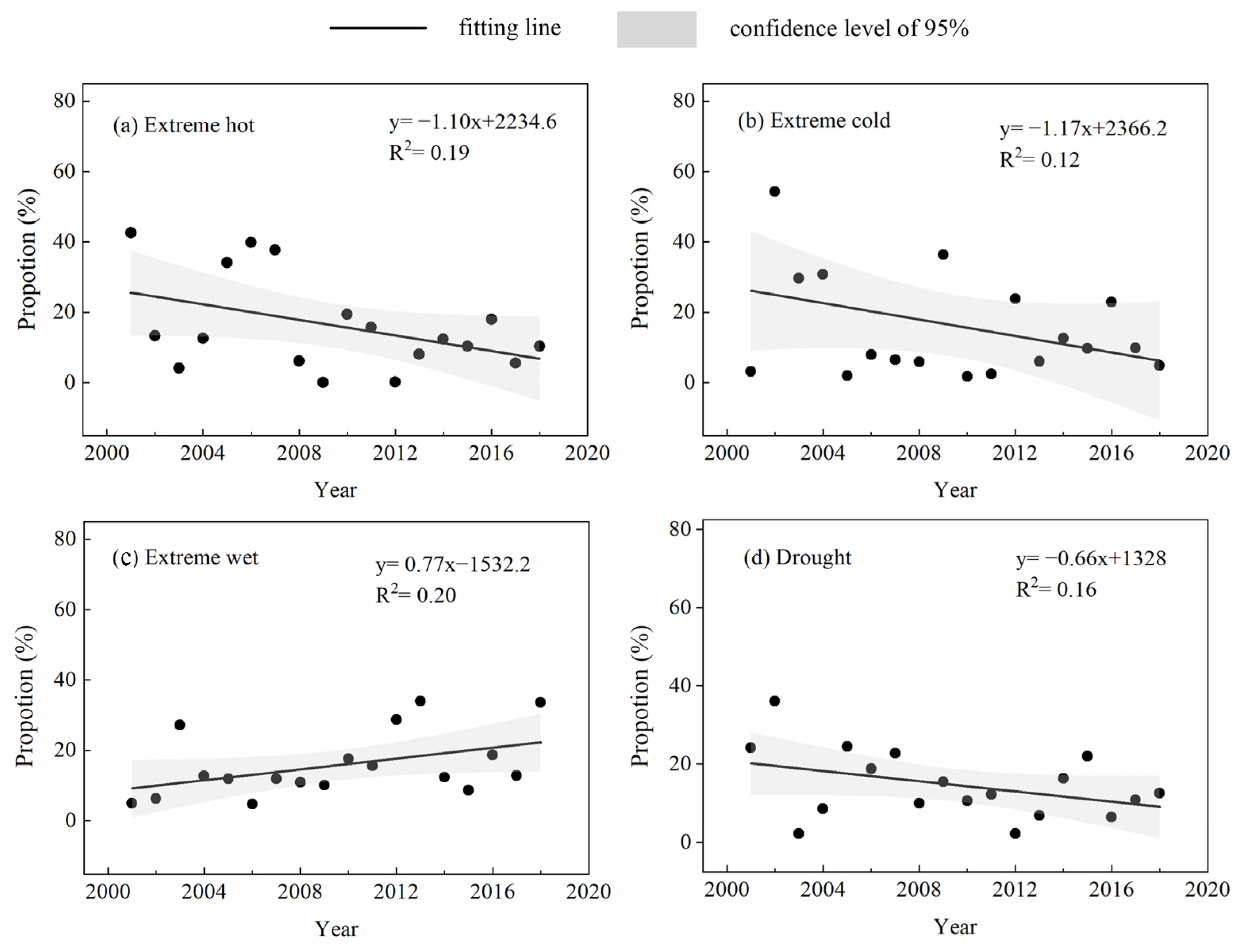
3.1. Temporal Variations in ECEs and EOS Anomalies

We explored the spatial distribution and change in the areas affected by ECEs and EOS anomalies (Figure 2 and Figure 3). The multiyear mean proportion of the affected areas was highest for extreme hot events (16.16%), followed by extreme cold events (16.14%), extreme wet events (15.72%) and extreme dry events (14.57%). Regarding changes in the proportion of affected areas, the proportion of extreme hot and extreme dry events exhibited a marginally significant (p = 0.06 and p = 0.07) decreasing trend of 1.10% and 0.66% per year, respectively. In contrast, extreme wet events showed a marginally significant increase of 0.77% per year (p = 0.06). Unlike these events, the change in the proportion of areas affected by extreme cold events was not significant (p = 0.16).

We analyzed the temporal variation in EOS across NC and found that it exhibited notable spatial heterogeneity (Figure S2). In total, 69.11% of the areas exhibited a trend towards delayed EOS, with 10.21% being significant (p < 0.05). The delayed EOS was mainly distributed in eastern Inner Mongolia. On the contrary, advanced EOS was predominantly observed in northeastern China and the northern Tibetan Plateau. Across the entire study region, EOS exhibited a delaying trend at a rate of 0.25 days/a during the period 2001–2018. For EOS anomalies, no significant trend (p > 0.1) was observed in either negative or positive EOS anomalies (Figure 3).

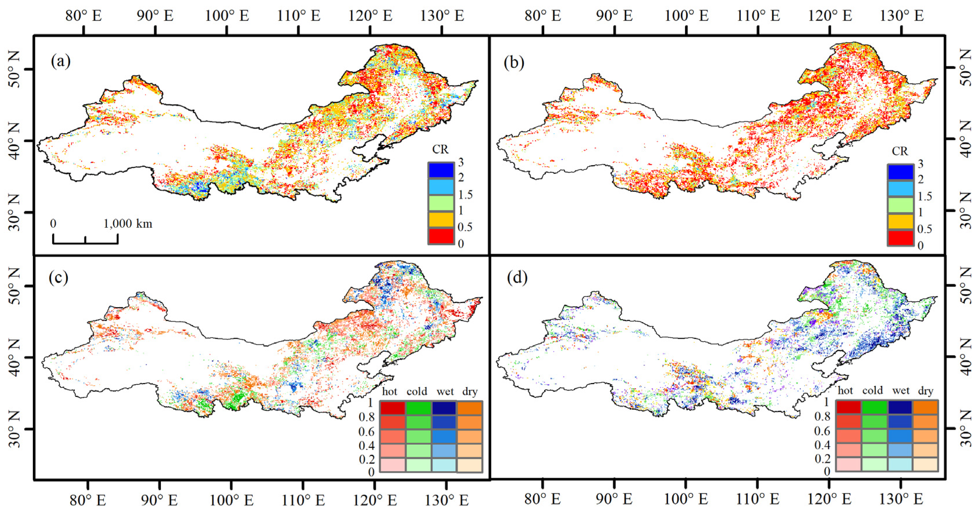
3.2. CR between ECEs and EOS Anomalies

We compared the spatial distribution of CR between ECEs and EOS anomalies based on 1 and 1.5 STD and found a similar spatial pattern for both (Table S1, Figures S3 and S4). Therefore, we used only the CR based on 1 STD in the subsequent analyses.

The CR between negative EOS anomalies and ECEs, calculated using the original sequence of ECEs, was significantly larger in 87.31% of the pixels compared to the values obtained by randomly shuffling the ECEs time series (Figure S5). Similarly, for positive EOS anomalies, the observed CR in 72.52% of the pixels was significantly greater than that derived from the shuffled sequence. These findings suggest that EOS anomalies and ECEs were not randomly associated, indicating a strong relationship between EOS anomalies and ECEs.

Spatial heterogeneity in the total rate of coincidence was observed for each EOS anomaly (Figure 4) Negative EOS anomalies exhibited high coincidence with all ECEs, with the total CR exceeding 0.5 in 73.33% of the pixels. This coincidence was particularly pronounced in regions near the Tibetan Plateau, where the total CR exceeded 1. In contrast, positive EOS anomalies exhibited a lower coincidence with ECEs, with the total CR below 0.5 in 67.80% of the pixels. In addition, no distinct spatial variation was detected in CR for positive EOS anomalies.

Among the extreme events, the CRs between the negative EOS anomalies and extreme dry (CR_{dry_N}), hot (CR_{hot_N}), cold (CR_{cold_N}) and wet (CR_{wet_N}) events were 0.31, 0.28, 0.24 and 0.14, respectively (Figure 5). This result indicated that extreme dry, hot and cold events were more closely related to negative EOS anomalies compared to extreme wet events. Spatially, the effects of these events varied across regions and vegetation types (Figure 4). For instance, extreme dry events substantially impacted negative EOS anomalies in steppes and meadows, where most CR_{dry_N} values exceeded 0.3. Extreme hot events dominated the occurrence of negative EOS anomalies in 28.30% of pixels, especially in broadleaf forests and steppes. In 22.11% of the pixels, particularly in the meadow biome, extreme cold events had a greater impact on EOS anomalies than other events. In contrast to the aforementioned climate events, extreme wet events were more closely relevant to the occurrence of positive EOS anomalies, with a mean CR_{wet_P} of 0.23. This vital effect was primarily observed in the eastern regions and at the edge of the Tibetan Plateau.

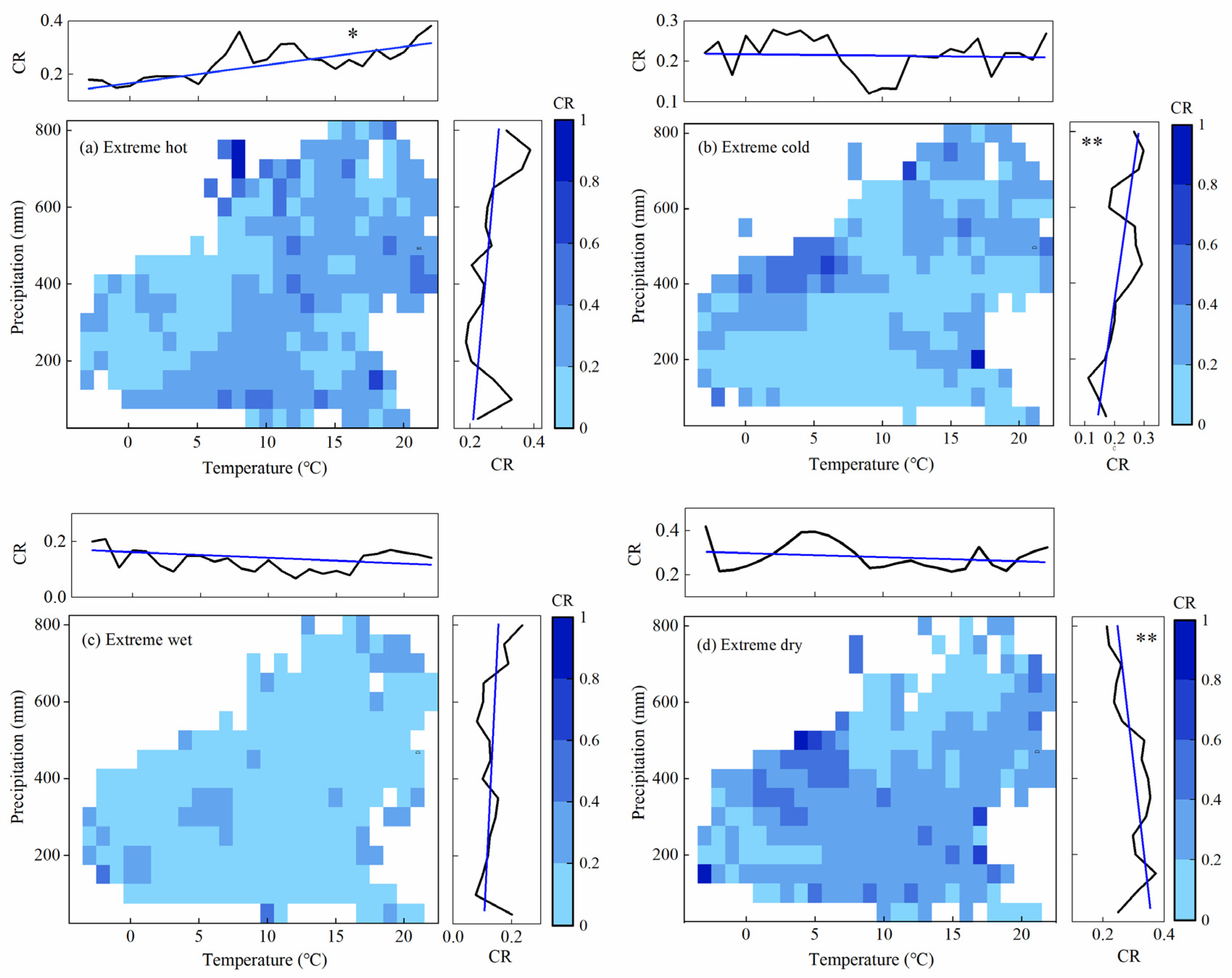
3.3. Dependency of CR on Local Climate Conditions

We found that CR_{hot_N}, CR_{cold_N} and CR_{dry_N} displayed a distinct pattern along the preseason temperatures or precipitation gradients (Figure 6). Specifically, an increase in the preseason temperature was markedly associated with a higher CR_{hot_N}, indicating that the early EOS events were more affected by heat stress in warmer regions. CR_{cold_N} and CR_{dry_N} were significantly associated with preseason precipitation, with CR_{cold_N} showing a positive and CR_{dry_N} showing a negative correlation. Oppositely, for CR_{wet_N}, the correlations with local climates were found to be insignificant, implying the absence of a clear pattern in the negative effect of extreme wet events on EOS along the local climate. In the case of the CR between positive EOS anomalies and ECEs, CR_wet-P exhibited a significant positive correlation with precipitation, meaning the extreme wet events resulted in more delayed EOS events in wetter regions (Figure 7). However, the CRs for other ECEs (i.e., CR_hot-P, CR_cold-P and CR_dry-P) did not exhibit clear tendencies along temperature or precipitation gradients, suggesting that the response of positive EOS anomalies to these climate events were less influenced by background climate conditions.

We further analyzed the CRs between EOS anomalies and the relevant ECEs across the hydrothermal conditions for each vegetation type. This analysis aimed to investigate the consistency and variation in the susceptibilities of EOS to ECEs across different biomes.

Figure 8 shows the CRs for each climate event in all biomes, and we found that CRs varied among biomes. Specifically, the CR_{hot_N} of broadleaf forests (CR_{hot_N} = 0.31) was higher than that of steppes (CR_{hot_N} = 0.28), meadows (CR_{hot_N} = 0.27) and coniferous forests (CR_{hot_N} = 0.22), indicating that the EOS in broadleaf forests was more susceptible to extreme hot events compared to that in other biomes. Additionally, extreme wet events emerged as a more crucial factor for EOS in forests (CR_{wet_P} = 0.26) than in grasslands (CR_{wet_P} = 0.21). In contrast, the CR_{cold_N} and CR_{dry_N} were higher in steppes and meadows, suggesting that extreme cold and extreme dry events exerted a profound impact on EOS in grasslands.

The dependency pattern of CRs on background climates was generally consistent across vegetation types (Figure 8). Specifically, a higher CR_{hot_N} was observed in warmer regions, while CR_{cold_N} and CR_{wet_P} increased with rising precipitation. For extreme dry events, it exhibited mild variations in CR across biomes. To be specific, broadleaf forests and steppes showed a decreasing trend in CR_{dry_N} with increasing precipitation, whereas the other two biomes did not exhibit a distinct trend along precipitation gradients.

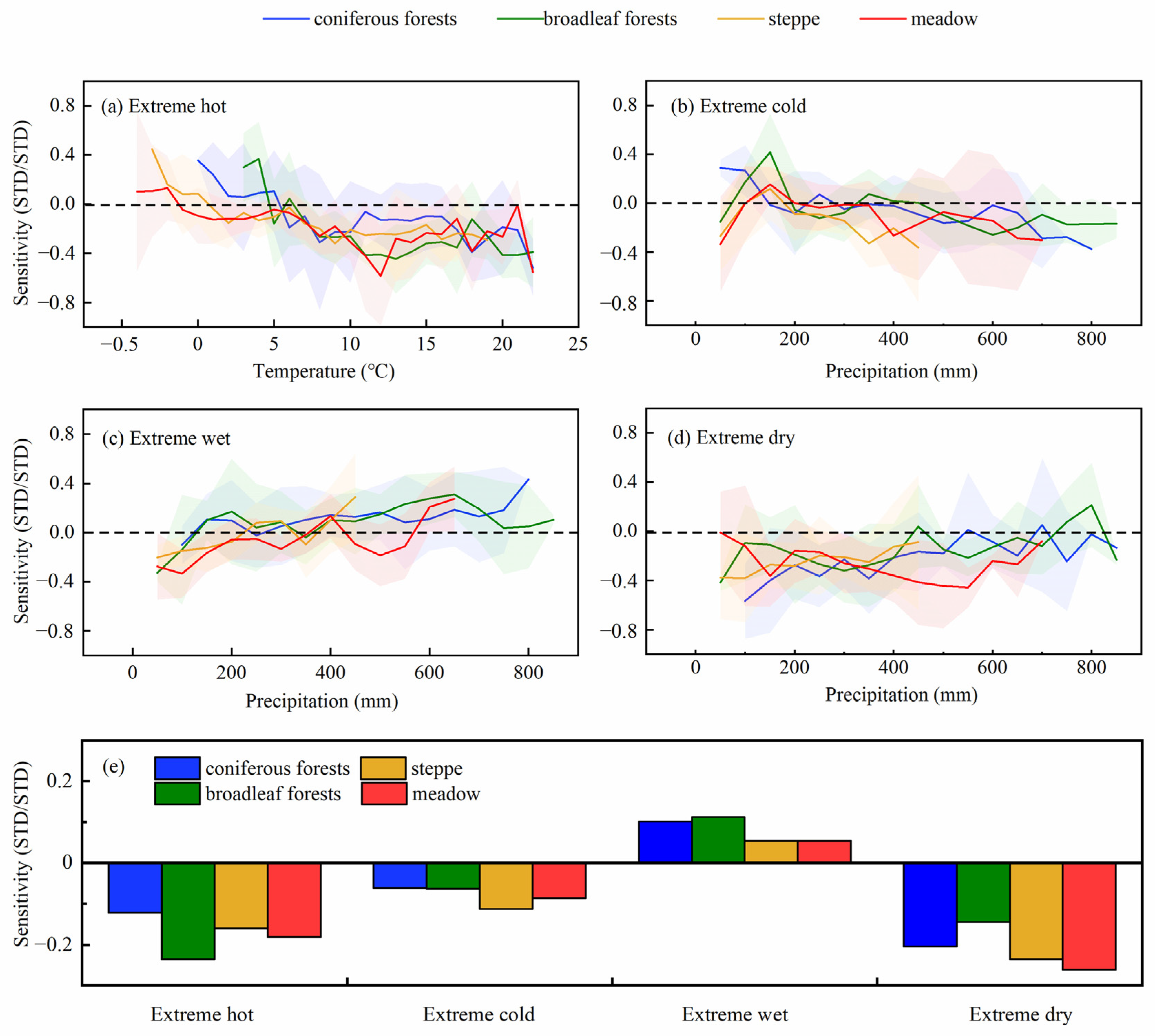
3.4. Sensitivity of EOS to ECEs

The sensitivities of EOS to ECEs across various background hydrothermal conditions are illustrated in Figure 9. We observed that the sensitivity of EOS to extreme heat (St_hot) was initially positive and gradually decreased with rising temperature in regions with temperatures below 5 °C. In areas with temperatures exceeding 5 °C, St_hot reversed to negative. This result indicates that the advancement effect of hot events was higher in warmer regions. St_cold was positive in regions with precipitation below 200 mm. Conversely, in areas with more than 200 mm of precipitation, St_cold reversed to negative and decreased with increasing precipitation, that is, extreme cold events accelerated EOS, and this effect became more prominent with higher precipitation levels. In the case of the sensitivity of EOS to extreme wet events, St_wet continued to increase with increasing precipitation, implying that EOS was more sensitive to extreme cold events in wetter areas. Regarding St_dry, it remained consistently negative for all vegetation types but varied among biomes along precipitation gradients. Specifically, the St_dry in forests and steppes increased with higher precipitation levels, while the St_dry in meadows showed no distinct trend along the precipitation gradient. This observation suggests that the negative impact of drought events on EOS in forests and steppes diminished with increasing precipitation, while the EOS response to drought events in meadows showed no clear pattern along the precipitation gradient. These findings indicate that the pattern of the sensitivities of EOS to ECEs across various temperature and precipitation gradients closely resembles the pattern of CRs, further suggesting that CR patterns may be influenced by the sensitivities of EOS to extreme climate conditions.

For the variations in the sensitivity of EOS to ECEs across different vegetation types (Figure 9), EOS in grasslands responded more sensitively to extreme dry (St = −0.25), hot (St = −0.16) and cold (St = −0.09), while the EOS in forests was more susceptible to extreme wet events (St = 0.11).

4. Discussion

4.1. Changes in ECEs and EOS

In this study, we found that extreme cold events and extreme hot events in preseason, i.e., generally summer and autumn, slightly decreased over 2001–2018. Since extreme cold and extreme hot events were characterized by a minimum temperature and maximum temperature, respectively, this finding suggests that the temperature increase was more prominent at night than during the day. Our findings align with the global diurnal asymmetric warming in recent years, with stronger nighttime warming compared to daytime warming on the global land surface [47]. In terms of moisture conditions, we observed that extreme wet events slightly increased, while drought occurrences decreased, which supports the fact that prolonged droughts have reduced in frequency and precipitation has displayed more significant fluctuations in grasslands in northern China [24]. In addition to summer and autumn, significant changes in climate extremes have also occurred during spring and winter. For instance, cold events have diminished, while heat events have become more prevalent during these seasons in temperate China [38]. Additionally, drought events in winter and spring have shown an increasing trend across most of China [51]. These extreme climate changes in the spring and winter seasons can affect phenology and should not be ignored.

Consistent with the previous studies in China that identified a delaying trend in autumn phenology [52,53], our findings similarly reveal a delayed EOS and an expansion of areas experiencing delayed EOS events from 2001 to 2018 in Northern China. These delayed EOS and increased EOS anomalies suggest an extension of the growing season, which could potentially enhance vegetation productivity and carbon assimilation [54,55]. For instance, a delay of 3 d yr⁻¹ in leaf senescence would lead to an increase of 5 g C m⁻² yr⁻¹ in net ecosystemic productivity in late summer in forests [56]. Given the ongoing climate warming and associated increase in extreme climate events, vegetation phenology is expected to change significantly [18]. Therefore, it is crucial to examine the effects of extreme climates on the shifts in EOS and further assess the functions and sustainability of terrestrial ecosystems [1,57].

4.2. Regulation of Background Climates on the Response of EOS to ECEs

We found that extreme dry and extreme hot events were the primary drivers of EOS anomalies in Northern China, which corroborates previous reports demonstrating that drought and heat stresses had a noticeable influence on autumn phenology in many temperate areas [30,58]. We observed that the negative effects of extreme drought and hot events on EOS were more pronounced in drier and warmer regions, respectively. Consistent with our study, existing studies also highlight the strong dependence of the EOS response to extreme climates on local hydrothermal conditions. For instance, a previous study found that drought was the main factor contributing to the advancement of EOS in warm regions in alpine and temperate grasslands of China [59].Moreover, recent research suggested that advancement in leaf senescence due to drought was predominantly observed in warmer and drier regions [22]. Several factors may explain these phenomena. First, the study regions are characterized by higher evapotranspiration and lower soil moisture. High evapotranspiration between the saturated leaf interior and the ambient air could lead to stomata closure and prevent excessive xylem pressure [60], further severely limiting photosynthesis and carbon assimilation [61]. Second, abscisic acid, which regulates the activities of antioxidant enzymes and mitigates cellular damage under high-temperature conditions, may become less effective under frequent extreme heat, resulting in delayed EOS [24]. Lastly, heat stress can also catalyze protein degradation in plants [19,62], accelerating leaf senescence [63,64].

At the community level, we found that grasslands, including steppes and meadows, were more susceptible to extreme hot and extreme dry events compared to forests. The finding is consistence with other studies suggesting that autumn phenology in grasslands exhibits a more pronounced response to heat and drought stresses than in forests [30,65]. The disparity in responses to heat events between forests and grasslands may be attributed to the fact that high temperatures could accelerate the evaporation of plants, leading to increased soil water loss [39], and this effect is more pronounced in grasslands, which primarily grow in drier environments. Consequently, grasslands are more sensitive to extreme hot events than forests. In terms of the response to drought events, the difference between forests and grasslands may be related to the species-specific physiological structures. Water availability plays a limiting factor for plant growth in arid environments [66]. Herbs typically have shallower roots and thus primarily absorb water at the surface soil layer [67]. Therefore, they are more vulnerable to drought events [68]. By contrast, deep-rooted plants, such as forest trees, are less likely to be affected by water stress due to their ability to access deeper water reserves [69,70]. Accordingly, forests are less susceptible and exhibit slower responses to drought events compared to grasslands [71,72].

We found that the influence of extreme cold events on early EOS events was more pronounced in high-precipitation regions across all vegetation types. This observation aligns with the finding that wet and cold conditions at high altitudes facilitate earlier EOS in Central Asia [30]. The underlying reason may be the elevated autumnal frost damage due to higher moisture levels at low temperatures, which increases the risk of injury to plant cells and tissues, leading to earlier leaf discoloration [29,73]. On the other hand, high soil moisture in colder areas could limit nutrient availability to plants, thereby constraining plant growth [74]. Consistent with previous studies demonstrating a higher sensitivity of shrubland to extreme cold compared with forests in arid areas [30], we observed that grasslands were more susceptible to cold events than woody plants. This is likely because the low temperatures in grasslands act as a limiting factor, thereby enhancing the susceptibility of herbs to frost damage [75]. Furthermore, the greater accumulation of antifreeze proteins, cryoprotective compounds and sugars and higher productivity in forests may contribute to their lower sensitivity to cold stress [76]. For instance, studies have shown that higher sugar levels in forest vegetation help modulate tissue osmolality and retain the stability of the leaf membranes under low temperatures [11,77].

In the present study, extreme wet events generally resulted in delayed EOS, and the susceptibility of EOS to extreme wet events increased under wetter conditions. This finding supports the evidence of positive sensitivities of autumn phenology to excessive wetness in drylands [78]. This phenomenon may be attributed to the typically dry conditions of the target region, where increased precipitation could significantly mitigate these dry conditions [79]. Interestingly, the coincidence rates between extreme wet events and delayed EOS events for coniferous forests decreased when precipitation exceeded approximately 700 mm (Figure 8c). This reduction may be due to the high soil moisture in coniferous forests, which creates an anaerobic environment in the plant root zone under excess precipitation, thereby inhibiting vegetation growth [80,81].

4.3. Limitations of the Study

The study has several limitations. First, the relatively coarse spatial resolution of satellite data and the uncertainty in phenological metrics extraction algorithms may have contributed to inaccuracies in phenology data. Thus, higher spatial resolution satellite data and optimized approaches for extracting phenology information are urgently needed. Additionally, autumn phenology can be influenced by other factors, such as solar radiation, atmospheric CO₂ levels [82], and nutrient availability [83]. However, accounting for all these factors in large-scale remote sensing applications is challenging due to their number and complexity. Consequently, the study focused solely on the key drivers, i.e., extreme temperature events and extreme precipitation events, which are well recognized for their substantial impact on phenology. Future research should consider additional climatic and ecological factors to provide a more comprehensive understanding of changes in autumn phenological events. Moreover, this study concentrated on individual extreme climate events, overlooking the potential effects of compound extreme climate events on vegetation phenology. However, compound extreme events might exert more profound impacts on ecosystems than their univariate counterparts [18]. Future research on the effects of compound extreme events, utilizing a combination of remote sensing and in situ data collected through field sampling and experiments, is essential to enhancing our understanding of the mechanisms underlying autumn phenological responses to climate change.

5. Conclusions

Using the EOS time series extracted from MODIS NDVI and EVI, we examined the response of autumn phenology to extreme climate events in Northern China. Our analysis revealed a slight decrease in the areas experiencing extreme heat and dry events and a slight increase in the areas experiencing extreme wet events from 2001 to 2018. In addition, we observed a delaying trend of EOS during the study period. The susceptibility of EOS to ECEs was closely related to local hydrothermal conditions, with higher susceptibility to extreme dry and extreme hot events in drier and warmer areas and higher susceptibility to extreme cold and extreme wet events in wetter regions. Among the vegetation types, grasslands were more sensitive to extreme dry, hot and cold events, whereas forests were more susceptible to extreme wet events. This study enhances our comprehension of the autumn phenological response to multiple extreme climates across various biomes and local hydrothermal environments. Future field manipulative experiments focusing on additional climatic factors and compound extreme climates are necessary to further understand the mechanisms underlying the autumn phenology response to climate change.

References

1. Piao, S.; Liu, Q.; Chen, A.; Janssens, I.A.; Fu, Y.; Dai, J.; Liu, L.; Lian, X.; Shen, M.; Zhu, X. Plant phenology and global climate change: Current progresses and challenges. Glob. Change Biol. 2019, 25, 1922–1940. [Google Scholar] [CrossRef] [PubMed]
2. Richardson, A.D.; Keenan, T.F.; Migliavacca, M.; Ryu, Y.; Sonnentag, O.; Toomey, M. Climate change, phenology, and phenological control of vegetation feedbacks to the climate system. Agric. For. Meteorol. 2013, 169, 156–173. [Google Scholar] [CrossRef]
3. Chen, H.; Zhao, J.; Zhang, H.; Zhang, Z.; Guo, X.; Wang, M. Detecting the response characteristics and thresholds of grassland spring phenology to climatic factors in the Mongolian Plateau. Ecol. Indic. 2023, 153, 110440. [Google Scholar]
4. Körner, C.; Möhl, P.; Hiltbrunner, E. Four ways to define the growing season. Ecol. Lett. 2023, 26, 1277–1292. [Google Scholar] [CrossRef]
5. Li, Y.; Zhang, W.; Schwalm, C.R.; Gentine, P.; Smith, W.K.; Ciais, P.; Kimball, J.S.; Gazol, A.; Kannenberg, S.A.; Chen, A.; et al. Widespread spring phenology effects on drought recovery of Northern Hemisphere ecosystems. Nat. Clim. Change 2023, 13, 182–188. [Google Scholar] [CrossRef]
6. Piao, S.; Wang, X.; Park, T.; Chen, C.; Lian, X.; He, Y.; Bjerke, J.W.; Chen, A.; Ciais, P.; Tømmervik, H.; et al. Characteristics, drivers and feedbacks of global greening. Nat. Rev. Earth Environ. 2020, 1, 14–27. [Google Scholar] [CrossRef]
7. Fu, Y.; He, H.S.; Zhao, J.; Larsen, D.R.; Zhang, H.; Sunde, M.G.; Duan, S. Climate and Spring Phenology Effects on Autumn Phenology in the Greater Khingan Mountains, Northeastern China. Remote Sens. 2018, 10, 449. [Google Scholar] [CrossRef]
8. Liu, Q.; Fu, Y.; Zhu, Z.; Liu, Y.; Liu, Z.; Huang, M.; Janssens, I.; Piao, S. Delayed autumn phenology in the Northern Hemisphere is related to change in both climate and spring phenology. Glob. Change Biol. 2016, 22, 3702–3711. [Google Scholar] [CrossRef]
9. Olsson, C.; Jönsson, A.M. A model framework for tree leaf colouring in Europe. Ecol. Model. 2015, 316, 41–51. [Google Scholar] [CrossRef]
10. Ren, P.; Liu, Z.; Zhou, X.; Peng, C.; Xiao, J.; Wang, S.; Li, X.; Li, P. Strong controls of daily minimum temperature on the autumn photosynthetic phenology of subtropical vegetation in China. For. Ecosyst. 2021, 8, 31. [Google Scholar] [CrossRef]
11. Bao, G.; Jin, H.; Tong, S.; Chen, J.; Huang, X.; Bao, Y.; Shao, C.; Mandakh, U.; Chopping, M.; Du, L. Autumn phenology and its covariation with climate, spring phenology and annual peak growth on the mongolian plateau. Agric. For. Meteorol. 2021, 298, 108312. [Google Scholar] [CrossRef]
12. Caparros-Santiago, J.A.; Rodriguez-Galiano, V.; Dash, J. Land surface phenology as indicator of global terrestrial ecosystem dynamics: A systematic review. ISPRS J. Photogramm. Remote Sens. 2021, 171, 330–347. [Google Scholar] [CrossRef]
13. Wang, X.; Wu, C.; Liu, Y.; Peñuelas, J.; Peng, J. Earlier leaf senescence dates are constrained by soil moisture. Glob. Change Biol. 2022, 29, 1557–1573. [Google Scholar] [CrossRef] [PubMed]
14. Gallinat, A.S.; Primack, R.B.; Wagner, D.L. Autumn, the neglected season in climate change research. Trends Ecol. Evol. 2015, 30, 169–176. [Google Scholar] [CrossRef]
15. Vitasse, Y.; Baumgarten, F.; Zohner, C.M.; Rutishauser, T.; Pietragalla, B.; Gehrig, R.; Dai, J.; Wang, H.; Aono, Y.; Spark, T.H. The great acceleration of plant phenological shifts. Nat. Clim. Change 2022, 12, 300–302. [Google Scholar] [CrossRef]
16. Wu, C.; Peng, J.; Ciais, P.; Peñuelas, J.; Wang, H.; Beguería, S.; Andrew Black, T.; Jassal, R.S.; Zhang, X.; Yuan, W.; et al. Increased drought effects on the phenology of autumn leaf senescence. Nat. Clim. Change 2022, 12, 943–949. [Google Scholar] [CrossRef]
17. Crabbe, R.A.; Dash, J.; Rodriguez-Galiano, V.F.; Janous, D.; Pavelka, M.; Marek, M.V. Extreme warm temperatures alter forest phenology and productivity in europe. Sci. Total Environ. 2016, 563, 486–495. [Google Scholar] [CrossRef]
18. Hao, Z. Compound events and associated impacts in China. iScience 2022, 25, 104689. [Google Scholar] [CrossRef]
19. Zhong, R.; Yan, K.; Gao, S.; Yang, K.; Zhao, S.; Ma, X.; Zhu, P.; Fan, L.; Yin, G. Response of grassland growing season length to extreme climatic events on the Qinghai-Tibetan Plateau. Sci. Total Environ. 2024, 909, 168488. [Google Scholar] [CrossRef]
20. Deng, H.; Yin, Y.; Han, X. Vulnerability of vegetation activities to drought in Central Asia. Environ. Res. Lett. 2020, 15, 084005. [Google Scholar] [CrossRef]
21. Li, P.; Liu, Z.; Zhou, X.; Xie, B.; Li, Z.; Luo, Y.; Zhu, Q.; Peng, C. Combined control of multiple extreme climate stressors on autumn vegetation phenology on the Tibetan Plateau under past and future climate change. Agric. For. Meteorol. 2021, 308, 108571. [Google Scholar] [CrossRef]
22. Bai, W.; Wang, H.; Dai, J.; Ge, Q. Changes in peak greenness timing and senescence duration codetermine the responses of leaf senescence date to drought over Mongolian grassland. Agric. For. Meteorol. 2024, 345, 109869. [Google Scholar] [CrossRef]
23. Ge, W.; Han, J.; Zhang, D.; Wang, F. Divergent impacts of droughts on vegetation phenology and productivity in the Yungui Plateau, southwest China. Ecol. Indic. 2021, 127, 107743. [Google Scholar] [CrossRef]
24. Zhao, Z.; Wang, X.; Li, R.; Luo, W.; Wu, C. Impacts of climate extremes on autumn phenology in contrasting temperate and alpine grasslands in China. Agric. For. Meteorol. 2023, 336, 109495. [Google Scholar] [CrossRef]
25. Xie, Y.; Wang, X.; Silander, J.A., Jr. Deciduous forest responses to temperature, precipitation, and drought imply complex climate change impacts. Proc. Natl. Acad. Sci. USA 2015, 112, 13585–13590. [Google Scholar] [CrossRef]
26. Zeppel, M.J.B.; Wilks, J.V.; Lewis, J.D. Impacts of extreme precipitation and seasonal changes in precipitation on plants. Biogeosciences 2014, 11, 3083–3093. [Google Scholar] [CrossRef]
27. Peng, J.; Wu, C.; Zhang, X.; Wang, X.; Gonsamo, A. Satellite detection of cumulative and lagged effects of drought on autumn leaf senescence over the Northern Hemisphere. Glob. Change Biol. 2019, 25, 2174–2188. [Google Scholar] [CrossRef]
28. Ren, P.; Li, P.; Tang, J.; Li, T.; Liu, Z.; Zhou, X.; Peng, C. Satellite monitoring reveals short-term cumulative and time-lag effect of drought and heat on autumn photosynthetic phenology in subtropical vegetation. Environ. Res. 2023, 239, 117364. [Google Scholar] [CrossRef]
29. Xie, Y.; Wang, X.; Wilson, A.M.; Silander, J.A., Jr. Predicting autumn phenology: How deciduous tree species respond to weather stressors. Agric. For. Meteorol. 2018, 250, 127–137. [Google Scholar] [CrossRef]
30. Gao, X.; Tao, Z.; Dai, J. Significant influences of extreme climate on autumn phenology in Central Asia grassland. Ecol. Indic. 2023, 155, 111056. [Google Scholar] [CrossRef]
31. Ying, H.; Zhang, H.; Zhao, J.; Shan, Y.; Zhang, Z.; Guo, X.; Rihan, W.; Deng, G. Effects of spring and summer extreme climate events on the autumn phenology of different vegetation types of Inner Mongolia, China, from 1982 to 2015. Ecol. Indic. 2020, 111, 105974. [Google Scholar] [CrossRef]
32. Berdugo, M.; Delgado-Baquerizo, M.; Soliveres, S.; Hernández-Clemente, R.; Zhao, Y.; Gaitán, J.J.; Gross, N.; Saiz, H.; Maire, V.; Lehmann, A.; et al. Global ecosystem thresholds driven by aridity. Science 2020, 367, 787–790. [Google Scholar] [CrossRef] [PubMed]
33. Donges, J.F.; Schleussner, C.F.; Siegmund, J.F.; Donner, R.V. Event coincidence analysis for quantifying statistical interrelationships between event time series. Eur. Phys. J. Spec. Top. 2016, 225, 471–487. [Google Scholar] [CrossRef]
34. Baumbach, L.; Siegmund, J.F.; Mittermeier, M.; Donner, R.V. Impacts of temperature extremes on European vegetation during the growing season. Biogeosciences 2017, 14, 4891–4903. [Google Scholar] [CrossRef]
35. Zhang, Y.; Hong, S.; Liu, D.; Piao, S. Susceptibility of vegetation low-growth to climate extremes on Tibetan Plateau. Agric. For. Meteorol. 2023, 331, 109323. [Google Scholar] [CrossRef]
36. Liu, D.; Wang, T.; Yang, T.; Yan, Z.; Liu, Y.; Zhao, Y.; Piao, S. Deciphering impacts of climate extremes on Tibetan grasslands in the last fifteen year. Sci. Bull. 2019, 64, 446–454. [Google Scholar] [CrossRef]
37. Duo, A.; Zhao, W.; Qu, X.; Jing, R.; Xiong, K. Spatio-temporal variation of vegetation coverage and its response to climate change in North China plain in the last 33 years. Int. J. Appl. Earth Obs. Geoinf. 2016, 53, 103–117. [Google Scholar]
38. Mo, Y.; Zhang, X.; Liu, Z.; Zhang, J.; Hao, F.; Fu, Y. Effects of Climate Extremes on Spring Phenology of Temperate Vegetation in China. Remote Sens. 2023, 15, 686. [Google Scholar] [CrossRef]
39. He, Z.; Du, J.; Chen, L.; Zhu, X.; Lin, P.; Zhao, M.; Fang, S. Impacts of recent climate extremes on spring phenology in arid-mountain ecosystems in China. Agric. For. Meteorol. 2018, 260–261, 31–40. [Google Scholar] [CrossRef]
40. Wu, J.; Zheng, X.; Zhao, L.; Fan, J.; Liu, J. Effects of ecological programs and other factors on soil wind erosion between 1981–2020. Remote Sens. 2022, 14, 5322. [Google Scholar] [CrossRef]
41. Xie, T.; Ding, T.; Wang, J.; Zhang, Y.; Gao, H.; Zhao, X.; Zhao, L. Weather pattern conducive to the extreme summer heat in North China and driven by atmospheric teleconnections. Environ. Res. Lett. 2023, 18, 104025. [Google Scholar] [CrossRef]
42. Zhang, Y.; Hao, Z.; Feng, S.; Zhang, X.; Hao, F. Changes and driving factors of compound agricultural droughts and hot events in eastern China. Agric. Water Manag. 2022, 263, 107485. [Google Scholar] [CrossRef]
43. He, J.; Yang, K.; Tang, W.; Lu, H.; Qin, J.; Chen, Y.Y.; Li, X. The first high-resolution meteorological forcing dataset for land process studies over China. Sci. Data 2020, 7, 25. [Google Scholar] [CrossRef] [PubMed]
44. Yang, K.; Jie, H.; Tang, W.; Qin, J.; Cheng, C. On downward shortwave and longwave radiations over high altitude regions: Observation and modeling in the Tibetan plateau. Agric. For. Meteorol. 2010, 150, 38–46. [Google Scholar] [CrossRef]
45. Peng, J.; Wu, C.; Wang, X.; Lu, L. Spring phenology outweighed climate change in determining autumn phenology on the Tibetan Plateau. Int. J. Climatol. 2021, 41, 3725–3742. [Google Scholar] [CrossRef]
46. Chen, J.; Jonsson, P.; Tamura, M.; Gu, Z.H.; Matsushita, B.; Eklundh, L. A simple method for reconstructing a high quality NDVI time-series data set based on the Savitzky-Golay filter. Remote Sens. Environ. 2004, 91, 332–344. [Google Scholar] [CrossRef]
47. Wu, C.; Wang, X.; Wang, H.; Ciais, P.; Peñuelas, J.; Myneni, R.B.; Desai, A.R.; Gough, C.M.; Gonsamo, S.; Black, A.T.; et al. Contrasting responses of autumn-leaf senescence to daytime and night-time warming. Nat. Clim. Change 2018, 8, 1092–1096. [Google Scholar] [CrossRef]
48. Piao, S.; Fang, J.; Zhou, L.; Ciais, P.; Zhu, B. Variations in satellite-derived phenology in china’s temperate vegetation. Glob. Change Biol. 2006, 12, 672–685. [Google Scholar] [CrossRef]
49. Elmore, A.J.; Guinn, S.M.; Minsley, B.J.; Richardson, A.D. Landscape controls on the timing of spring, autumn, and growing season length in mid-Atlantic forests. Glob. Change Biol. 2012, 18, 656–674. [Google Scholar] [CrossRef]
50. Guo, M.; Wu, C.; Peng, J.; Lu, L.; Li, S. Identifying contributions of climatic and atmospheric changes to autumn phenology over mid-high latitudes of Northern Hemisphere. Glob. Planet. Change 2021, 197, 103396. [Google Scholar] [CrossRef]
51. Tao, Z.; Dai, J.; Wang, X.; Wang, Y. Influence of Early-Season Drought on the Peak of Growing Season in China Varies by Drought Timing and Biomes. Forests 2024, 15, 1027. [Google Scholar] [CrossRef]
52. Gao, X.; Dai, J.; Tao, Z.; Shahzad, K.; Wang, H. Autumn phenology of tree species in China is associated more with climate than with spring phenology and phylogeny. Front. Plant Sci. 2023, 14, 1040758. [Google Scholar] [CrossRef] [PubMed]
53. Ge, Q.; Wang, H.; Rutishauser, T.; Dai, J. Phenological response to climate change in China: A meta-analysis. Glob. Change Biol. 2015, 21, 265–274. [Google Scholar] [CrossRef] [PubMed]
54. Chen, S.; Fu, Y.H.; Hao, F.; Li, X.; Zhou, S.; Liu, C.; Tang, J. Vegetation phenology and its ecohydrological implications from individual to global scales. Geogr. Sustain. 2022, 3, 334–338. [Google Scholar] [CrossRef]
55. Lv, Y.; Zhang, L.; Li, P.; He, H.; Ren, X.; Xie, Z.; Wang, Y.; Wang, A.; Shi, F.; Chang, R.; et al. Improving Phenology Representation of Deciduous Forests in the Community Land Model: Evaluation and Modification Using Long-Term Observations in China. J. Adv. Model. Earth Syst. 2023, 15, e2023MS003655. [Google Scholar] [CrossRef]
56. Dragoni, D.; Rahman, A.F. Trends in fall phenology across the deciduous forests of the Eastern USA. Agric. For. Meteorol. 2012, 157, 96–105. [Google Scholar] [CrossRef]
57. Ren, S.; Qin, Q.; Ren, H.; Sui, J.; Zhang, Y. New model for simulating autumn phenology of herbaceous plants in the Inner Mongolian Grassland. Agric. For. Meteorol. 2019, 275, 136–145. [Google Scholar] [CrossRef]
58. Wang, M.; Li, P.; Peng, C.; Xiao, J.; Zhou, X.; Luo, Y.; Zhang, C. Divergent responses of autumn vegetation phenology to climate extremes over northern middle and high latitudes. Glob. Ecol. Biogeogr. 2022, 31, 2281–2296. [Google Scholar] [CrossRef]
59. Yuan, Z.; Tong, S.; Bao, G.; Chen, J.; Yin, S.; Li, F.; Sa, C.; Bao, Y. Spatiotemporal variation of autumn phenology responses to preseason drought and temperature in alpine and temperate grasslands in China. Sci. Total Environ. 2023, 859, 160373. [Google Scholar] [CrossRef]
60. Yuan, W.; Zheng, Y.; Piao, S.; Ciais, P.; Lombardozzi, D.; Wang, Y.; Ryu, Y.; Chen, G.; Dong, W.; Hu, Z.; et al. Increased atmospheric vapor pressure deficit reduces global vegetation growth. Sci. Adv. 2019, 5, eaax1396. [Google Scholar] [CrossRef]
61. McDowell, N.; Pockman, W.T.; Allen, C.D.; Breshears, D.D.; Cobb, N.; Kolb, T.; Plaut, J.; Sperry, J.; West, A.; Williams, D.G.; et al. Mechanisms of plant survival and mortality during drought: Why do some plants survive while others succumb to drought? New Phytol. 2008, 178, 719–739. [Google Scholar] [CrossRef] [PubMed]
62. Gulen, H.; Eris, A. Effect of heat stress on peroxidase activity and total protein content in strawberry plants. Plant Sci. 2004, 166, 739–744. [Google Scholar] [CrossRef]
63. Fracheboud, Y.; Luquez, V.; Bjorken, L.; Sjodin, A.; Tuominen, H.; Jansson, S. The control of autumn senescence in European aspen. Plant Physiol. 2009, 149, 1982–1991. [Google Scholar] [CrossRef] [PubMed]
64. Ueda, T.; Seo, S.; Ohashi, Y.; Hashimoto, J. Circadian and senescence-enhanced expression of a tobacco cysteine protease gene. Plant Mol. Biol. 2000, 44, 649–657. [Google Scholar] [CrossRef]
65. Sun, M.; Li, X.; Xu, H.; Wang, K.; Anniwaer, N.; Hong, S. Drought thresholds that impact vegetation reveal the divergent responses of vegetation growth to drought across China. Glob. Change Biol. 2024, 30, e16998. [Google Scholar] [CrossRef]
66. Ji, H.; Yang, G.; Lv, X.; Jia, B.; Xu, Z.; Wang, Y. Climate extremes drive the phenology of a dominant species in meadow steppe under gradual warming. Sci. Total Environ. 2023, 869, 161687. [Google Scholar] [CrossRef]
67. An, S.; Chen, X.; Zhang, X.; Lang, W.; Ren, S.; Xu, L. Precipitation and minimum temperature are primary climatic controls of alpine grassland autumn phenology on the Qinghai-Tibet Plateau. Remote Sens. 2020, 12, 431. [Google Scholar] [CrossRef]
68. Propastin, P.; Kappas, M.; Muratova, N.R. Inter-annualchanges in vegetation activities and their relationship totemperature and precipitation in central asia from 1982 to 2003. J. Environ. Inform. 2008, 12, 75–87. [Google Scholar] [CrossRef]
69. Schwinning, S.; Davis, K.; Richardson, L.; Ehleringer, J.R. Deuterium enriched irrigation indicates different forms of rain use in shrub/grass species of the Colorado Plateau. Oecologia 2002, 130, 345–355. [Google Scholar] [CrossRef]
70. Müller, P.; Li, X.P.; Niyogi, K.K. Non-photochemical quenching. A response to excess light energy. Plant Physiol. 2001, 125, 1558–1566. [Google Scholar] [CrossRef]
71. Davis, S.D.; Mooney, H.A. Comparative water relations of adjacent California shrub and grassland communities. Oecologia 1985, 66, 522–529. [Google Scholar] [CrossRef] [PubMed]
72. Zhai, D.; Gao, X.; Li, B.; Yuan, Y.; Li, Y.; Liu, W.; Xu, J. Diverse chronic responses of vegetation aboveground net primary productivity to climatic changes on Three-River Headwaters region. Ecol. Indic. 2022, 139, 108925. [Google Scholar] [CrossRef]
73. Cong, N.; Shen, M.; Piao, S. Spatial variations in responses of vegetation autumn phenology to climate change on the Tibetan Plateau. J. Plant Ecol. 2017, 10, 744–752. [Google Scholar] [CrossRef]
74. Fu, Y.H.; Piao, S.; Delpierre, N.; Hao, F.; Hänninen, H.; Liu, Y.; Sun, W.; Janssens, I.; Campioli, M. Larger temperature response of autumn leaf senescence than spring leaf-out phenology. Glob. Change Biol. 2018, 24, 2159–2168. [Google Scholar] [CrossRef]
75. Shen, X.; Jiang, M.; Lu, X. Diverse impacts of day and night temperature on spring phenology in freshwater marshes of the Tibetan Plateau. Limnol. Oceanogr. Lett. 2022, 8, 323–329. [Google Scholar] [CrossRef]
76. Yuan, M.; Wang, L.; Lin, A.; Liu, Z.; Qu, S. Variations in land surface phenology and their response to climate change in Yangtze River basin during 1982–2015. Theor. Appl. Climatol. 2018, 137, 1659–1674. [Google Scholar] [CrossRef]
77. Gusta, L.V.; Wisniewski, M. Understanding plant cold hardiness: An opinion. Physiol. Plant. 2013, 147, 4–14. [Google Scholar] [CrossRef]
78. Wu, L.; Zhao, C.; Li, J.; Yan, Y.; Han, Q.; Li, C.; Zhu, J. Impact of extreme climates on land surface phenology in Central Asia. Ecol. Indic. 2023, 146, 109832. [Google Scholar] [CrossRef]
79. Yuan, M.; Zhao, L.; Lin, A.; Wang, L.; Li, Q.; She, D.; Qu, S. Impacts of preseason drought on vegetation spring phenology across the Northeast China Transect. Sci. Total Environ. 2020, 738, 140297. [Google Scholar] [CrossRef]
80. Li, P.; Zhu, Q.; Peng, C.; Zhang, J.; Wang, M.; Zhang, J.; Ding, J.; Zhou, X. Change in autumn vegetation phenology and the climate controls from 1982 to 2012 on the Qinghai–Tibet Plateau. Front. Plant Sci. 2020, 10, 1677. [Google Scholar] [CrossRef]
81. Yang, Y.; Guan, H.; Shen, M.; Liang, W.; Jiang, L. Changes in autumn vegetation dormancy onset date and the climate controls across temperate ecosystems in China from 1982 to 2010. Glob. Change Biol. 2015, 21, 652–665. [Google Scholar] [CrossRef] [PubMed]
82. Orsenigo, S.; Mondoni, A.; Rossi, G.; Abeli, T. Some like it hot and some like it cold, but not too much: Plant responses to climate extremes. Plant Ecol. 2014, 215, 677–688. [Google Scholar] [CrossRef]
83. Estiarte, M.; Penuelas, J. Alteration of the phenology of leaf senescence and fall in winter deciduous species by climate change: Effects on nutrient proficiency. Glob. Change Biol. 2015, 21, 1005–1017. [Google Scholar] [CrossRef] [PubMed]
Figure 1. Spatial distribution of mean annual temperature (a), mean annual precipitation (b), elevation (c) and vegetation types (Source: The Vegetation Maps of China with a proportional scale of 1:1,000,000) (d) in Northern China.
Remotesensing 16 03724 g001
Figure 2. Trends in the proportion of areas affected by extreme climate events in the preseason period during 2001–2018. The lines represent the linear fitting lines and the shaded areas are the 95% confidence bands of the fits.
Remotesensing 16 03724 g002
Figure 3. Trends in the proportion of areas experiencing EOS anomalies during 2001–2018. The lines represent the linear fitting lines and the shaded areas are the 95% confidence bands of the fits.
Remotesensing 16 03724 g003
Figure 4. Spatial distributions of the coincidence rates (CRs) between EOS anomalies and extreme climatic events (ECEs) in Northern China. (a) Total CR between the negative EOS anomalies and ECEs. (b) Total CR between the positive EOS anomalies and ECEs. (c) The CRs between the negative EOS anomalies and individual ECEs. (d) The CRs between the positive EOS anomalies with individual ECEs. Only climate extremes with the highest CRs are displayed at each pixel in (c,d).
Remotesensing 16 03724 g004
Figure 5. Percentage of the pixels of coincidence rates (CRs) between EOS anomalies and extreme climate extremes (ECEs) and the averaged CR for each ECE. The dark and light colors indicate the CRs are significant and non-significant, respectively.
Remotesensing 16 03724 g005
Figure 6. Distribution in the coincidence rates (CRs) between the negative EOS anomalies and extreme climate extremes along the preseason climate gradients. The black lines in the panels above and to the right of heat maps indicate the mean CRs against the preseason temperature in each bin of 1 °C or preseason precipitation in each bin of 50 mm, respectively. The blue lines represent the linear fitting lines of CRs. ** p < 0.01. * p < 0.05. Pixels that occur less than ten times within a 1 °C and 50 mm precipitation range were excluded to ensure the reliability.
Remotesensing 16 03724 g006
Figure 7. Distribution in the coincidence rates (CRs) between positive EOS anomalies and extreme climate extremes along the preseason climate gradients. The black lines in the panels above and to the right of heat maps indicate the mean CRs against the preseason temperature in each bin of 1 °C or preseason precipitation in each bin of 50 mm, respectively. The blue lines represent the linear fitting lines of CRs. ** p < 0.01. Pixels that occur less than ten times within a 1 °C and 50 mm precipitation range were excluded to ensure the reliability.
Remotesensing 16 03724 g007
Figure 8. Distribution of coincidence rates (CRs) between EOS anomalies and extreme climate extremes along preseason temperature and precipitation gradients. (a) CR of negative EOS anomalies and extreme hot events. (b) CR of negative EOS anomalies and extreme cold events. (c) CR of positive EOS anomalies and extreme wet events. (d) CR of negative EOS anomalies and extreme dry events. The shaded areas show the standard deviation. Note: Pixels that were fewer than 10 occurrences within a 1 °C temperature and a 50 mm precipitation range were excluded to ensure the reliability.
Remotesensing 16 03724 g008
Figure 9. Distribution in sensitivity of EOS to extreme climate events of four vegetation types along preseason temperature and precipitation gradients. The shaded areas represent the standard deviation. Note: Pixels that were fewer than 10 occurrences within a 1 °C temperature and a 50 mm precipitation range were excluded to ensure reliability.
Remotesensing 16 03724 g009
Disclaimer/Publisher’s Note: The statements, opinions and data contained in all publications are solely those of the individual author(s) and contributor(s) and not of MDPI and/or the editor(s). MDPI and/or the editor(s) disclaim responsibility for any injury to people or property resulting from any ideas, methods, instructions or products referred to in the content.