Automated Recognition of Snow-Covered and Icy Road Surfaces Based on T-Net of Mount Tianshan

Abstract

The Tianshan Expressway plays a crucial role in China’s “Belt and Road” strategy, yet the extreme climate of the Tianshan Mountains poses significant traffic safety risks, hindering local economic development. Efficient detection of hazardous road surface conditions (RSCs) is vital to address these challenges. The complexity and variability of RSCs in the region, exacerbated by harsh weather, make traditional surveillance methods inadequate for real-time monitoring. To overcome these limitations, a vision-based artificial intelligence approach is urgently needed to ensure effective, real-time detection of dangerous RSCs in the Tianshan road network. This paper analyzes the primary structures and architectures of mainstream neural networks and explores their performance for RSC recognition through a comprehensive set of experiments, filling a research gap. Additionally, T-Net, specifically designed for the Tianshan Expressway engineering project, is built upon the optimal architecture identified in this study. Leveraging the split-transform-merge structure paradigm and asymmetric convolution, the model excels in capturing detailed information by learning features across multiple dimensions and perspectives. Furthermore, the integration of channel, spatial, and multi-head attention modules enhances the weighting of key features, making the T-Net particularly effective in recognizing the characteristics of snow-covered and icy road surfaces. All models presented in this paper were trained on a custom RSC dataset, compiled from various sources. Experimental results indicate that the T-Net outperforms fourteen once state-of-the-art (SOTA) models and three models specifically designed for RSC recognition, with 97.44% accuracy and 9.79% loss on the validation set.

1. Introduction

The Tianshan Expressway is a critical transportation artery in Xinjiang, which plays a crucial role in the economic development of the region. Furthermore, the perennial snow accumulation in the Tianshan region, accounting for one-third of China’s snow resources, significantly exacerbates snow and ice hazards on the roadways. From October to March, extreme weather phenomena such as snowfall, snow accumulation, and blowing snow, as well as ice formation in mountainous areas, pose severe risks to transportation, human lives, and property. These conditions represent a significant meteorological hazard, disrupting the normal operation of expressways in Northern Xinjiang during the cold season and significantly impacting local economic development. Therefore, it is imperative to develop an effective method for the real-time surveillance of road surface conditions (RSCs) on the Tianshan Expressway.

In recent years, various methods for RSC recognition have been proposed, which can be categorized into contact and non-contact approaches [1]. Contact approaches primarily rely on embedded sensors, including capacitive sensors [2,3,4,5], fiber optic sensors [6,7], and resonant sensors [8]. Although these detection devices typically achieve high accuracy on clean surfaces, the presence of various types of impurities on road surfaces can significantly affect measurement accuracy. Additionally, the installation and maintenance of contact sensors require cutting the road surface, potentially disrupting traffic flow and reducing the lifespan of the road. As a result, capacitive, optical, and resonant methods have been applied within a restricted scope of RSC recognition. Non-contact approaches primarily rely on light sources and photoelectric detectors, including polarization detection [9,10,11], infrared detection [12,13], and multi-wavelength detection [14]. These optical detection technologies position the light source device at a certain height near the road and fix the light receiving device on the opposite side, using a wired transmission method. The high costs of installation, communication, and maintenance, coupled with substantial power consumption, make dense installation of these systems along road sections challenging, thereby also limiting their applicability in certain scenarios.

Recent advancements in deep learning have led to the emergence of camera-based approaches [15,16,17,18,19,20,21,22,23,24,25]. This non-contact method, relying on camera images for RSC recognition, has achieved higher accuracy compared to traditional methods. Pan et al. conducted a comparative study on the performance of four convolutional neural network (CNN) models (VGG16, ResNet50, Inception-v3, and Xception) in addressing RSC recognition problems, identifying ResNet50 as the optimal model for recognizing winter RSCs [15]. Dewangan et al., proposed a CNN-based network for complex scene road recognition called RCNet [18]. Huang et al., developed a transfer-learning model based on Inception-v3 for RSC recognition and used a residual neural network to segment flooded road areas [20]. Yang et al., tackled the challenges of complex and variable road scenes, low recognition rates of traditional machine-learning methods, and poor generalization capability by proposing an RSC-recognition algorithm based on residual neural networks [22]. Chen et al. addressed the issues of high cost and limited detection range in conventional hardware-based RSC-detection technologies by proposing a high-speed RSC detection method based on a U-Net fusion model [25].

Despite the fact that deep-learning models for RSC recognition have shown promise, most rely on pre-trained architectures with only superficial adjustments, such as the integration of attention mechanisms. However, the selection of these models is often not well justified, lacking rigorous comparisons with alternative structures or architectures. Most of them are trained on public datasets such as ImageNet and CIFAR. Therefore, it is crucial to compare their performances on specific RSC datasets, as they may not be suitable for RSC recognition. Current research has largely overlooked a comprehensive evaluation of various neural network designs for RSC recognition, which is a critical gap in the field. Addressing this gap is essential for advancing the development of more robust and effective RSC recognition systems. Given this situation, this study aims to develop a more effective method for recognizing RSCs on the Tianshan Expressway, which is crucial for enhancing road safety. The main contributions of the research are summarized as follows.

• A custom dataset covering six types of RSCs was compiled by using highway cameras, mobile lenses, and online resources. Subsequently, illumination correction and standardization processing were implemented to ensure compatibility with deep-learning models. In view of the scarcity of publicly available standardized datasets of road surface meteorological conditions internationally and the relative shortage of picture resources of road surface conditions in extreme weather, this dataset has contributed invaluable resources for improving the accuracy of the RSC recognition models.
• To overcome the limitations of existing RSC recognition methods, a novel model, T-Net, was proposed. It adopts a split-transform-merge paradigm with four distinct branching blocks, multiple attention mechanisms, and three trainable classification heads, allowing it to capture the diversity and complexity of the RSCs. Meanwhile, in order to fill the research gap and answer the question of which structure or architecture of the deep-learning model should be selected for an RSC recognition scenario, the performance differences of deep learning neural networks with different structures and architectures were explored and analyzed.
• The T-Net constructed is particularly beneficial for engineers and policymakers focused on road safety and transportation infrastructure in extreme climates such as those common in the Tianshan region. By exploring various combinations in convolution methods, attention mechanisms, loss functions, and optimizers, this study offers practical solutions for real-time RSC recognition, bridging the gap between theoretical research and practical application.

The remainder of this paper is organized as follows: Section 2 outlines the development of classical image recognition neural networks and RSC recognition models, Section 3 describes the preparation of the dataset and the architecture of the T-Net model, Section 4 provides the experimental settings and results, Section 5 presents a comprehensive discussion based on experimental outcomes, and Section 6 gives a summary of the paper.

2. Related Work

From our perspective, the latest networks are not always superior to older ones. Although new network architectures typically introduce more advanced algorithms and technologies, they do not consistently achieve superior performance in certain scenarios. Performance depends on various factors, including the complexity of the task, characteristics of the dataset, and the adaptability of the model. Therefore, a review of existing neural network architectures and RSC recognition models was conducted in preparation for the subsequent experiments in this section.

2.1. Different Features and Structures of Neural Networks

The rapid advancement of neural networks began in 2012 with the advent of deep-learning techniques and advancements in computational resources, which led to significant breakthroughs in computer vision. In the field of image recognition, neural networks can be categorized as follows:

From a design philosophy and core mechanism perspective, neural networks can be classified into two primary types: CNN-based and transformer-based. In CNN-based neural networks, two main design structures are prevalent. The first is the sequential (or chain) structure, typically formed by sequentially stacking a series of convolutional and pooling layers to create a linear network flow. Examples include AlexNet [26], VGG [27], ResNet [28], and others. The simplicity and intuitiveness of this structure render it facile to understand and implement. Notably, ResNet introduced residual connections, laying the foundation for deeper convolutional neural networks. The second type is the multi-branch structure, also known as the Inception structure. Xie et al. described this as a split-transform-merge model paradigm [29]. This structure uses multiple branches at the same level with different convolutional kernels or pooling operations, concatenating the output of each branch, as seen in GoogLeNet [30] and the Inception series [31,32]. The advantage of the multi-branch structure lies in its ability to simultaneously capture features at different scales and levels, enhancing the network’s expressive power. In transformer-based neural networks, although their design principles and mechanisms differ from CNN-based models, most still adopt a sequential connection structure. Examples include the Vision Transformer (ViT) [33], the Swin Transformer [34], and others. It is worth noting that the ViT represents a pioneering milestone by effectively integrating the self-attention mechanism from the transformer architecture into computer vision. Despite the fact that transformer-based models have demonstrated remarkable performance on benchmarks such as ImageNet, surpassing traditional CNNs and advancing the field of neural network research, they still encounter challenges, including a high number of parameters, demanding computational requirements, a lack of spatial inductive bias, limited adaptability to diverse tasks, and training complexities.

In terms of application scenarios, networks are mainly categorized as either standard or lightweight. Standard networks typically include models that excel on large-scale tasks, characterized by larger parameters and higher computational complexity. Examples include ResNet, ResNeXt, GoogLeNet, Inception, Inception-ResNet, ViT, ResViT, Swin Transformer, DenseNet [35], ConvNeXt [36], and others. Notably, ConvNeXt, proposed in 2022, demonstrates performance comparable to transformer-based networks when the convolutional architecture is well designed. In contrast, due to the increasing demand for neural networks in resource-constrained environments, studies [37,38,39,40,41,42,43,44] have increasingly focused on the development of lightweight neural networks. Recent examples specifically designed for mobile devices and embedded systems include MobileNet [40], EfficientNet [41], MobileViT [42], EfficientViT [43], and others. The core designs of MobileNet consist of depthwise separable convolution and width multipliers, which significantly reduce the computational cost and parameter count. EfficientNet achieves optimal performance through a compound scaling method. MobileViT adopts a hybrid CNN and transformer architecture, enhancing network convergence and inference speed through a CNN while incorporating spatial information through a transformer to improve network transferability. EfficientViT, the latest lightweight deep-learning model, incorporates a sandwich layout and cascaded group attention as fundamental components, surpassing existing efficient models and achieving an optimal balance between inference speed and accuracy.

Based on design approaches, neural networks can be divided into two major types: manually designed networks and neural architecture search (NAS) networks. Manual design of neural network architecture excels in flexibility and interpretability. Examples include GoogLeNet, DenseNet, ConvNeXt, and others. However, manual design is limited by the challenge of fully exploring potential data features, as effective neural network structure design requires significant expertise and experimentation. NAS methods aim to automate this process, providing more efficient discovery and optimization of neural network architectures. High-performance networks derived from NAS include MobileNet, EfficientNet, RegNet [44] and others. Although NAS methods have achieved good results, they also face several challenges, including high demands on computational resources, complexities in defining effective search spaces, uncertainties in performance evaluation, and limitations in generalization and applicability. Addressing these challenges is crucial for advancing NAS methods to enhance their efficiency and reliability in practical applications.

As discussed above, a wide range of neural network structures and architectures are used in image recognition, with key features and design methods outlined in

Table 1. Networks with different key features or design methods.

Classes	Model and Version	Key Feature or Design Method
Normal network	AlexNet [26]	sequential structure
	VGG [27]	sequential structure
	GoogLeNet [30]	multi-branch structure
	Inception [31]	multi-branch structure
	ResNet [28]	sequential structure with residual connection
	Inception-ResNet [32]	multi-branch structure with residual connection
	ResNeXt [29]	multi-branch structure with residual connection
	DenseNet [35]	sequential structure with dense connection
	ViT [33]	sequential structure with self-attention
	ResViT [33]	sequential structure with residual connection and self-attention
	Swin Transformer [34]	sequential structure with self-attention in shifted window
	ConvNeXt [36]	ResNet based on Swin Transformer design idea
Lightweight network	ShuffleNet [37,38]	hand-designed CNN architecture
	MobileNet [39,40]	NAS CNN architecture
	EfficientNet [41]	NAS CNN architecture
	RegNet [44]	NAS CNN architecture
	MobileViT [42]	hand-designed CNN-Transformer hybrid architecture
	EfficientViT [43]	NAS CNN-Transformer hybrid architecture

. However, many networks are optimized on datasets such as ImageNet and CIFAR, which do not necessarily guarantee good performance on other datasets. In practical applications, a suitable network architecture should be chosen based on a comprehensive consideration of task scenarios, data resources, computational resources, and other factors.

2.2. RSC Recognition Models

In recent years, deep learning neural networks for RSC recognition have gained widespread attention. In 2019, Pan et al., compared the performance of four CNN models (VGG16, ResNet50, Inception-v3, and Xception) to solve road condition classification problems. The results indicated that ResNet50 is the optimal model for classifying winter road surface conditions [15]. Yang et al. proposed an Inception-v3 model based on transfer learning to address the low accuracy of conventional methods for recognizing wet and dry RSC [16]. In 2020, Lee et al., introduced a convolutional network to identify black ice on roads to prevent traffic accidents of automated vehicles [17]. In 2021, Dewangan et al., developed the RCNet to tackle the challenges of complex scenes, varied road structures, and inappropriate lighting conditions on RSC recognition tasks [18]. In 2022, Wang et al., addressed the issue of low accuracy on RSC recognition tasks using an improved Inception-ResNet-v2 algorithm [19]. Huang et al., employed a transfer-learning model based on Inception-v3 for road surface slippery condition recognition and used a full-resolution residual network to segment waterlogged areas on roads [20]. Xie et al., developed a city RSC model using a pretrained CNN model to fill gaps in city highway condition recognition [21]. Yang et al., addressed the challenges of complex and variable road surface slippery condition recognition, low recognition rates of conventional machine-learning methods, and poor generalization capabilities by proposing a road surface slippery condition recognition algorithm based on high/low attention residual neural networks [22]. In 2023, Lee et al. constructed a deep-learning architecture for detecting black ice on roads using a pretrained ResNet-v2 and compared the performance of different models. The results showed that R101-FPN is the best model [23]. Kou et al., used a ResNeSt network for RSC recognition and proposed an active suspension control algorithm based on RSC recognition, improving performance of the suspension system effectively [24]. Chen et al., tackled the issues of high cost and limited detection range of conventional hardware-based RSC recognition technologies by proposing a high-speed RSC recognition method based on a U-Net fusion model [25].

While the aforementioned models have demonstrated significant advantages for RSC recognition, most of them rely on pretrained models and were fine-tuned on their specific datasets, or only minor modifications such as adding attention mechanisms were made to the original architectures. There is no reason why they chose that model. Notably, there is a clear research gap in the current body of work on road surface recognition, as few existing studies on road surface condition recognition have thoroughly investigated or compared the performance of different neural network structures and architectures from previous works.

3. Materials and Methods

3.1. Dataset

Based on statistical records of extreme weather conditions affecting traffic control on the Tianshan Expressway and the analysis of meteorological data obtained along the routes (available at https://cxfw.jtyst.xinjiang.gov.cn/home/index, accessed on 13 January 2024), the severity of ice and snow hazards on the Tianshan Expressway was categorized into road icing, blowing snow, and heavy snow. Given this situation, a custom dataset was compiled for the Tianshan Expressway using highway cameras, mobile lenses, and online resources. Among them, road icing and blowing snow, as extreme weather phenomena, have relatively low numbers. To ensure the balance of data samples and prevent the model from over-learning the features of a certain type, data augmentation was carried out for all to increase the number of images to 1500. The detailed sample size is shown in

Table 2. Distribution of dataset.

Road Categories	Dry	Fully Snowy	Icy	Snow-Blowing	Snow-Melting	Wet
Original	898	499	275	92	336	402
Augmentation	1500	1500	1500	1500	1500	1500
Sample size (MB)	28.6	17.2	36.0	19.8	38.1	27.6

. The dataset includes the following road surface types: (1) dry road; (2) fully snowy road; (3) icy road; (4) snow-blowing road; (5) snow-melting road; and (6) wet road. Examples of these data types are illustrated in Figure 1.

3.2. Data Preprocessing

Carrying out data augmentation prior to splitting the dataset into training, validation, and test sets may introduce potential correlations among these sets. This could undermine the independence of the validation and test sets, compromising the accuracy and reliability of model performance evaluations. To mitigate this issue, the dataset is firstly divided into three distinct sets and data augmentation is subsequently applied to each set independently. The specific processing steps are as follows:

• Data Resizing: The images were resized to 224 × 224 pixels, a standard size in deep learning due to its balance between computational efficiency and model performance. This size is widely used in pretrained models, such as those trained on ImageNet, and has proven successful in models such as the VGG and ResNet.
• Dataset split: The dataset was randomly divided into training, validation, and testing sets, comprising 60%, 20%, and 20% of the overall dataset, respectively.
• Adjustment of Brightness: Road surface conditions are often complex and variable, leading to issues such as occlusion between objects and non-uniform lighting. These problems manifest as regions of excessive brightness or darkness in images, which can obscure or blur critical details. Additionally, these factors can cause different types of road surfaces to appear similar, thereby increasing the difficulty of recognition. To address these challenges, an adaptive correction algorithm based on a two-dimensional gamma function was employed to adjust image illumination intensity [45]. The results of this correction are shown in Figure 2.
• Data Augmentation: Data augmentation is a crucial step for addressing dataset imbalance, where some labels have significantly more images than others. This method generates additional data from existing samples by applying transformations such as flipping, rotating, cropping, scaling, and color adjustments. In this study, the OpenCV and NumPy libraries were employed for data augmentation. By applying random flipping, random translation, random rotation, and Gaussian noise addition, the number of images was increased to 9000.
• Data Normalization: Pixel values were normalized to zero mean and unit standard deviation to accelerate model convergence. The mean values of the dataset were [0.550, 0.565, 0.568] and standard deviations were [0.082, 0.082, 0.085] for the red, green, and blue channels, respectively.

3.3. Network Architecture

T-Net employs a unique structural paradigm known as the split-transform-merge framework comprising four distinct Conv blocks, multiple attention mechanisms, and three classification heads. This framework aims to comprehensively capture the diversity of RSCs by leveraging information along different dimensions. The entire process of compressing and extracting information from feature image to linear tensor, including the changes in feature map dimensions and the number of channels, is illustrated in Figure 3. For example, given a 224 × 224 pixels image as input, after passing through Conv Block-1, the feature map size changes to 111 × 111, and the number of channels increases from the initial 3 channels (RGB) to 32. Subsequently, after passing through Conv Block-2 and Conv Block-3, the feature map becomes 109 × 109 × 64. Notably, each white “Out Layer” represents 32 channels. The codes and models used in this study can be accessed at https://github.com/Elijah0405/T-Net, accessed on 4 March 2024.

The intermediate sections of the model introduce a convolutional block attention module (CBAM) to enhance the focus on critical information after merging each branch. CBAM combines spatial and channel attention to improve the weighting of essential information throughout the model. Furthermore, T-Net incorporates asymmetric convolutions in the second and third branches to increase sensitivity to fine-grained details in images. Experimental results demonstrate the significant benefits of asymmetric convolutions in improving classification accuracy.

In the final classification stage, T-Net introduces an innovative feature that incorporates three distinct classification heads to compress information from multiple channels into six channels using various strategies. This design aims to enhance the model’s adaptability and performance. The first classification head combines the multi-head self-attention (MHSA) module with fully connected layers, allowing the model to effectively collaborate among multiple heads, each focusing on different features, thereby comprehensively capturing critical information. The second classification head integrates the CBAM with fully connected layers, further emphasizing crucial information and enhancing the model’s accuracy for RSC recognition. The third classification head relies solely on fully connected layers to facilitate information integration. Trainable coefficients are incorporated into each classification head, allowing the model to dynamically adjust these coefficients during training. This adaptability ensures superior performance under varying conditions. Detailed structural parameters of the model are listed in

Table 3. Structural parameters of T-Net.

Seq	Layers		Patch Size/Stride/Padding	Output Size
1	Conv1		3 × 3/2/0	111 × 111 × 32
2	Conv2		3 × 3/1/0	109 × 109 × 64
3	Conv3		3 × 3/1/1	109 × 109 × 64
4	Branch 1-1	MaxPool	3 × 3/2/0	54 × 54 × 64
5	Branch 1-2	AvgPool	3 × 3/2/0	54 × 54 × 64
6	Branch 1-3	Conv1	3 × 3/2/0	54 × 54 × 96
7	CBAM			54 × 54 × 224
8	Branch 2-1	Conv3	1 × 1/1/0	54 × 54 × 64
9		Conv2	3 × 3/1/0	52 × 52 × 96
10	Branch 2-2	Conv3	1 × 1/1/0	54 × 54 × 64
11		Conv4	7 × 1/1/3	54 × 54 × 64
12		Conv4	1 × 7/1/3	54 × 54 × 64
13		Conv2	3 × 3/1/0	52 × 52 × 96
14	CBAM			52 × 52 × 192
15	Branch 3-1	Conv1	3 × 3/2/0	25 × 25 × 96
16		Conv4	3 × 1/1/1	25 × 25 × 96
17		Conv4	1 × 3/1/1	25 × 25 × 96
18	Branch 3-2	Conv3	1 × 1/1/0	52 × 52 × 96
19		MaxPool	3 × 3/2/0	25 × 25 × 96
20	Branch 3-3	Conv3	1 × 1/1/0	52 × 52 × 96
21		AvgPool	3 × 3/2/0	25 × 25 × 96
22	Branch 3-4	Conv1	3 × 3/2/0	25 × 25 × 96
23	CBAM			25 × 25 × 384
24	Conv1		3 × 3/2/0	12 × 12 × 512
25	Branch 4-1	Transformer		1 × 1 × 512
26		Linear		1 × 1 × 6
27	Branch 4-2	CBAM		12 × 12 × 512
28		MaxPool	12 × 12/1/0	1 × 1 × 512
29		Linear		1 × 1 × 6
30	Branch 4-3	MaxPool	12 × 12/1/0	1 × 1 × 512
31		Linear		1 × 1 × 6

.

3.3.1. Conv Layer

Specifically, four Conv modules were designed, each comprising a convolution layer, normalization layer, and activation layer. Conv1 applies a 3 × 3 kernel with a stride of 2 to reduce image size and modify the number of channels. Conv2 employs a 3 × 3 kernel with a stride of 1 to increase the number of channels while reducing the image size by 2 pixels. Conv3 uses a 1 × 1 kernel to increase the number of channels. Conv4 utilizes an asymmetric kernel to extract fine-grained features. These modules are the key elements of the T-Net. The procedure applied by the Conv structures can be expressed as follows:

$$C\left(a,b\right)={\sum }_{p=1}^x{\sum }_{q=1}^{y}I\left(a+p-1,b+q-1\right)\times K(p,q)$$

(1)

$$\left\{\begin{array}{c}\mathrm{Mean} \left(\mathrm{M}\mathrm{i}\mathrm{n}\mathrm{i}\mathrm{b}\mathrm{a}\mathrm{t}\mathrm{c}\mathrm{h}\right):{\mu }_B={\displaystyle \frac{1}{m}}{\sum }_{i=1}^m{x}_i\\ \mathrm{Variance} \left(\mathrm{M}\mathrm{i}\mathrm{n}\mathrm{i}\mathrm{b}\mathrm{a}\mathrm{t}\mathrm{c}\mathrm{h}\right): {\sigma }_B^2={\displaystyle \frac{1}{m}}{\sum }_{i=1}^m{\left(x_i-{\mu }_B\right)}^2\\ {\mathrm{N}\mathrm{o}\mathrm{r}\mathrm{m}\mathrm{a}\mathrm{l}\mathrm{i}\mathrm{z}\mathrm{e}: \widehat{x}}_l={\displaystyle \frac{x_i-{\mu }_B}{\left.\sqrt{(}{\sigma }_B^2+ϵ\right)}}\\ {\mathrm{S}\mathrm{c}\mathrm{a}\mathrm{l}\mathrm{e}\&\mathrm{S}\mathrm{h}\mathrm{i}\mathrm{f}\mathrm{t}: y}_i=Y{\widehat{x}}_l+\beta =B{N}_{Y,\beta }\left(x_i\right)\end{array}\right.$$

(2)

$$ReLU=\max \left(0,x\right)=\left\{\begin{array}{c}0, x<0\\ x, x>0\end{array}\right.$$

(3)

Equation (1) represents the convolution process where $C(a,b)$ is the output result of the convolution operation at position $(a,b)$, while $I(a+p-1,b+q-1)$ is the input information of the image at position ($a+p-1,b+q-1$), where $a$ and $b$ iterate from 1 to X − x + 1 and Y − y + 1, respectively (with X being the image width and Y being the image height). $K(p,q)$ is the convolution parameter at position $(p,q)$, representing the weight learned during the training process. The summation over $p$ and $q$ indicates that the convolution kernel moves across the entire input image, generating new output values at position $(a,b)$ with each movement. The size of the kernel is determined by x and y.

The batch normalization process is expressed in Equation (2), where ${\mu }_B$ is the average value, m is the input minibatch, ${\sigma }_B^2$ is the variance, ${\widehat{x}}_l$ is the result of the normalization, and $Y$ and $\beta$ are the learnable parameters.

Equation (3) is the activation function, where $\mathrm{x}$ represents the input data. The derivative of the ReLU function is always equal to 1 in the positive region, avoiding the occurrence of a vanishing or exploding gradient problem.

3.3.2. Pooling Layer

The non-significant features can be diminished by applying a pooling operator with an average value or by mapping a subregion to its maximum value:

$$P_{\mathrm{avg}}(I)={\displaystyle \frac{1}{T}}{\sum }_{u=1}^T{i}_u$$

(4)

$$P_{\mathrm{m}\mathrm{a}\mathrm{x}}(I)=max{i}_u$$

(5)

where vector $i$ comprises the activation values from the respective pooling regions of T pixels in the image. In the downsampling strategy scenario presented here, Equation (5) is applied to the T-Net.

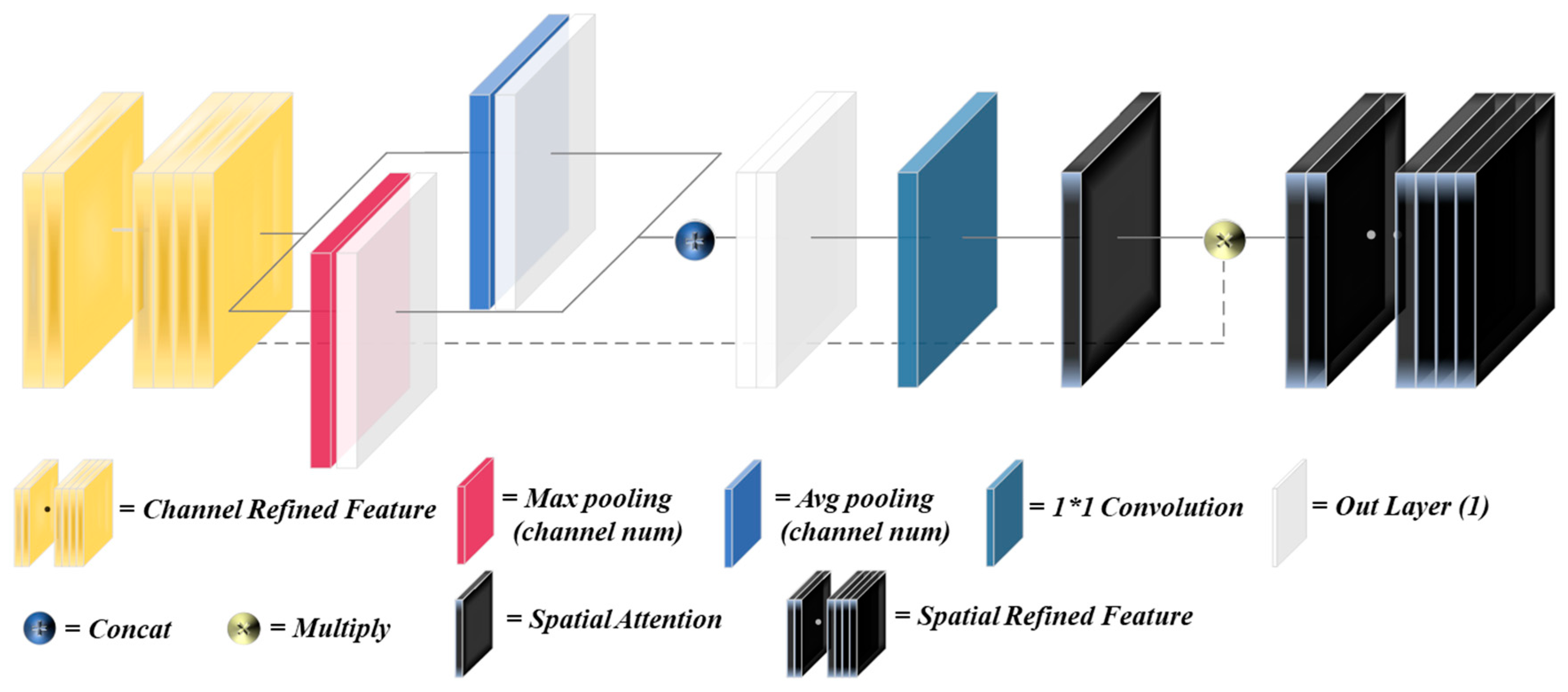
3.3.3. Channel and Spatial Attention

The channel and spatial attention mechanisms in T-Net are referred to as the convolutional block attention module (CBAM). The CBAM module, shown in Figure 4, Figure 5 and Figure 6, describes the calculation process for each attention map.

The overall computation process of the CBAM module can be summarized as follows:

$$\begin{array}{c}{\mathrm{F}}^{\prime }={\mathrm{M}}_{\mathrm{c}}\left(\mathrm{F}\right)\otimes \mathrm{F}\\ {\mathrm{F}}^{″}={\mathrm{M}}_{\mathrm{s}}\left({\mathrm{F}}^{\prime }\right)\otimes {\mathrm{F}}^{\prime }\end{array}$$

(6)

Given an intermediate feature map $\mathrm{F}\in {\mathbb{R}}^{C\times H\times W}$ as input, then the channel attention module generates a one-dimensional channel attention map $\mathrm{M}\mathrm{c}\in {\mathbb{R}}^{C\times 1\times 1}$, and the spatial attention module generates a two-dimensional spatial attention map $\mathrm{M}\mathrm{s}\in {\mathbb{R}}^{1\times H\times W}$. where $\otimes$ denotes element-wise multiplication.

In the channel attention module, the input feature map undergoes global average pooling and global max pooling separately. The results of average pooling and max pooling are then processed using a shared multilayer perceptron. The outputs of the shared multi-layer perceptron are summed and then passed through a sigmoid activation function to obtain the channel attention map, which provides weights ranging from 0 to 1 for each channel in the input feature map. Finally, the weights are applied to the input feature map through multiplication, channel-wise. The computation process of the channel attention mechanism can be expressed as follows:

$$\begin{array}{ll}{\mathrm{M}}_{\mathrm{c}}\left(\mathrm{F}\right)& =\sigma \left(MLP\right(\mathrm{A}\mathrm{v}\mathrm{g}\mathrm{P}\mathrm{o}\mathrm{o}\mathrm{l}\left(\mathrm{F}\right))+MLP(\mathrm{M}\mathrm{a}\mathrm{x}\mathrm{P}\mathrm{o}\mathrm{o}\mathrm{l}\left(\mathrm{F}\right)\left)\right)\\ & =\sigma \left({\mathrm{W}}_1\left({\mathrm{W}}_0\left({\mathrm{F}}_{\mathrm{avg}}^{\mathrm{c}}\right)\right)+{\mathrm{W}}_1\left({\mathrm{W}}_0\left({\mathrm{F}}_{\mathrm{m}\mathrm{a}\mathrm{x}}^{\mathrm{c}}\right)\right)\right)\end{array}$$

(7)

where $\sigma$ denotes the sigmoid function, ${\mathrm{W}}_0\in {\mathbb{R}}^{C/r\times C}$, and ${\mathrm{W}}_1\in {\mathbb{R}}^{C\times C/r}$.

In the spatial attention module, the input feature map undergoes average pooling and max pooling respectively along the channel dimensions. These results are stacked and passed through a standard convolutional layer to reduce the number of channels to 1. After applying the sigmoid activation function, a two-dimensional spatial attention map is generated, providing weights ranging from 0 to 1 for each spatial location in the input feature map. Finally, the weights are applied to the input feature map through element-wise multiplication. The specific calculation process is as follows:

$$\begin{array}{ll}{\mathrm{M}}_{\mathrm{s}}\left(\mathrm{F}\right)& =\sigma \left(f^{7\times 7}\left(\right[\mathrm{A}\mathrm{v}\mathrm{g}\mathrm{P}\mathrm{o}\mathrm{o}\mathrm{l}\left(\mathrm{F}\right);\mathrm{M}\mathrm{a}\mathrm{x}\mathrm{P}\mathrm{o}\mathrm{o}\mathrm{l}\left(\mathrm{F}\right)\left]\right)\right)\\ & =\sigma \left(f^{7\times 7}\left(\left[{\mathrm{F}}_{\mathrm{avg}}^{\mathrm{s}};{\mathrm{F}}_{\max }^{\mathrm{s}}\right]\right)\right)\end{array}$$

(8)

where $\sigma$ denotes the sigmoid function and $f^{7\times 7}$ represents a convolution operation with the filter size 7 × 7.

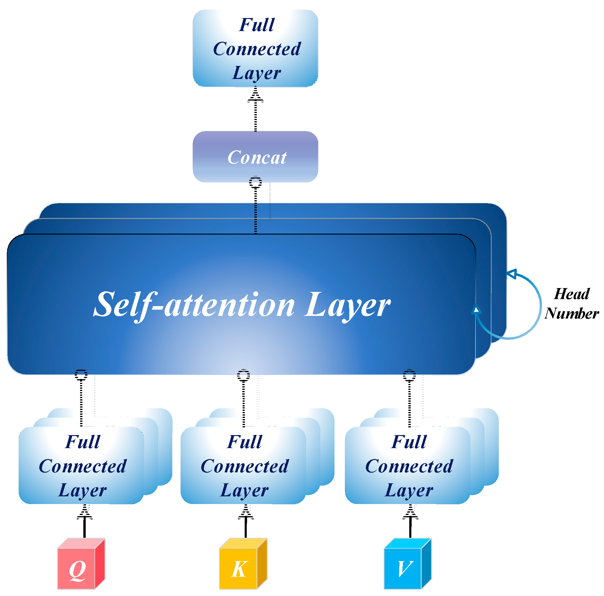
3.3.4. Multi-Head Self-Attention

Multi-head self-attention mechanisms are formed by a number of self-attention mechanisms, as illustrated in Figure 7 and expressed as follows:

$$\mathrm{M}\mathrm{u}\mathrm{l}\mathrm{t}\mathrm{i}\mathrm{H}\mathrm{e}\mathrm{a}\mathrm{d}(Q,K,V)=\mathrm{C}\mathrm{o}\mathrm{n}\mathrm{c}\mathrm{a}\mathrm{t}\left({\mathrm{h}\mathrm{e}\mathrm{a}\mathrm{d}}_1,\dots ,{\mathrm{h}\mathrm{e}\mathrm{a}\mathrm{d}}_h\right)W^O$$

(9)

where ${head}_i$ represents the attention mechanisms $\mathrm{A}\mathrm{t}\mathrm{t}\mathrm{e}\mathrm{n}\mathrm{t}\mathrm{i}\mathrm{o}\mathrm{n}\left(Q{W}_i^Q,K{W}_i^K,V{W}_i^V\right)$, with the trainable parameter matrices $W_i^Q\in {\mathbb{R}}^{d_{\mathrm{model}}\times d_k},W_i^K\in {\mathbb{R}}^{d_{\mathrm{model}}\times d_k},W_i^V\in {\mathbb{R}}^{d_{\mathrm{model}}\times d_v}$ and $W^O\in {\mathbb{R}}^{h{d}_v\times d_{\mathrm{model}}}$. Where $W_i^Q$, $W_i^K$, and $W_i^V$ are the query, key, and value transformation matrices for ${\mathrm{h}\mathrm{e}\mathrm{a}\mathrm{d}}_i$, and $W^O$ is the output transformation matrix. Each attention mechanism represents a distinct space, and multiple mechanisms enable the derivation of diverse representation spaces. Each mechanism utilizes unique Query, Key, and Value weight matrices, which are initialized randomly. Consequently, multi-head attention allows the model to collectively attend to information across various representation subspaces and positions.

4. Results

4.1. Performance Testing of Different Network Architectures for RSC Recognition

Comparative results of performance differences among various networks on the custom RSC dataset were presented in this section. Based on the neural network classifications described in Section 2.1, several network structures and architectures in different versions were selected, as detailed in

Table 4. Comparison with different structures and architectures networks.

Model and Version	#param. (M)	FLOPs (G)	Accuracy	Loss
VGG-16	134.29	15.48	90.50%	66.47%
Inception-v4	48.35	12.73	96.11%	19.74%
ResNet-18	11.18	1.81	94.50%	21.79%
ResNet-50	23.52	4.09	93.78%	22.40%
Inception-ResNet-v2	30.37	9.27	97.05%	11.12%
ResNeXt-50	22.99	4.23	96.39%	15.26%
DenseNet-121	6.96	2.83	96.89%	12.87%
ViT-base	85.80	0.20	90.44%	59.00%
Swin Transformer-base	86.75	0.18	87.67%	55.32%
ConvNeXt-base	87.57	0.65	93.00%	69.20%
T-Net	6.03	1.69	97.44%	9.79%
ShuffleNet-v2-x2	5.36	0.58	95.27%	15.18%
EfficientNet-b0	4.02	0.38	92.83%	29.50%
EfficientViT-m2	3.96	0.20	88.17%	36.99%
MobileNet-v3-large	4.21	0.22	93.39%	23.78%
MobileViT-small	4.94	0.85	94.17%	27.11%

. Various combinations of hyperparameters, including the number of epochs, learning rate, batch size, and weight decay, along with different optimizers such as SGD and Adam, were systematically explored. These efforts aimed to address overfitting and underfitting issues, ultimately optimizing the performance of each model. The loss function employed was cross-entropy loss, and the primary learning rate strategy was cosine decay. To further evaluate the effectiveness of these networks, key metrics such as parameter counts, FLOPs, accuracy, and loss were employed. The loss value, derived from the cross-entropy loss function, measures how closely the predicted probabilities align with the actual labels, with lower cross entropy indicating better alignment. Specifically, the training set loss reflects how well the model fits the training data, while the validation dataset loss indicates its ability to transfer and generalize to unseen data.

As shown in Table 4, the T-Net achieves the highest accuracy at 97.44% and the lowest loss at 9.79%, outperforming other models in both 6.03 M parameters and 1.69 GFLOPs. Inception-ResNet-v2 follows closely with an accuracy of 97.05% and a loss of 11.12%, but at the cost of greater model complexity, with 30.37 M parameters and 9.27 GFLOPs. DenseNet-121 ranks third, delivering a strong performance with 96.89% accuracy and 12.87% loss, while maintaining a relatively low parameter count of 6.96 M. Other high-performing models, such as the ResNeXt-50 and the Inception-v4, also achieve accuracies exceeding 96%, but with higher losses of 15.26% and 19.74%, respectively. In contrast, models such as the VGG-16, ViT-base, and ConvNeXt-base, which have large parameter sizes, tend to be less efficient and are more susceptible to overfitting, resulting in diminished performance. Figure 8 further highlights the superiority of the T-Net, with its performance curves consistently outperforming those of other models on both the training and validation sets, indicating that it has greater efficiency and generalization capabilities.

For lightweight networks, Table 4 demonstrates that the ShuffleNet-v2-x2 achieves the highest accuracy of 95.27% and the lowest loss of 15.18%. In contrast, the EfficientViT-m2 exhibits the lowest accuracy of 88.17% and the highest loss of 36.99%. Other models, such as the EfficientNet-b0, the MobileNet-v3-large, and the MobileViT-small, display accuracy and loss that fall between these extremes. As shown in Figure 9, despite the ShuffleNet-v2-x2 having a slower convergence trend on the training set, with its curve positioned further inward, it surpasses all other lightweight models on the validation set, indicating strong robustness and generalization capability. Contrary to the performance of the ShuffleNet-v2-x2, the EfficientViT-m2 performs well on the training set with the fastest convergence trend, but it performs the worst on the validation set.

4.2. Comparsion with Specilized RSC Recognition Networks

Based on the review in Section 2.2, three RSC classification models were selected for evaluation: RCNet, Inception-ResNet-v2 with SE module, and ResNet18 with high/low attention. Meanwhile, the original Inception-ResNet-v2 and ResNet18 were added for comparison. The experimental setup followed the guidelines outlined in Section 4.1.

As shown in

Table 5. Comparison with specialized RSC recognition neural networks.

Model and Version	#param. (M)	FLOPs (G)	Accuracy	Loss
RCNet	3.78	5.48	89.33%	33.32%
Inception-ResNet-v2 with SE module	31.87	8.62	97.39%	10.32%
Inception-ResNet-v2	30.37	9.27	97.05%	11.12%
ResNet18 with high/low attention	11.88	2.02	94.94%	17.84%
ResNet-18	11.18	1.81	94.50%	21.79%
T-Net	6.03	1.69	97.44%	9.79%

, the performance comparison highlights significant variations among the models in terms of accuracy, computational cost, and model complexity. The T-Net achieves the highest accuracy at 97.44% with the lowest loss of 9.79%, while maintaining a relatively low computational load of 1.69 GFLOPs and a parameter count of 6.0M. The Improved Inception-ResNet-v2 model, integrated with the SE module, demonstrates exceptional performance, achieving an accuracy of 97.39% and a loss of 10.32%. In comparison, the standard Inception-ResNet-v2 exhibits a slight decrease in accuracy to 97.05% and an increase in loss to 11.12%. The ResNet18 model, utilizing high/low attention, shows significant enhancements with an accuracy of 94.94% and a loss of 17.84%. This marks an improvement of 0.44% percentage points in accuracy and a reduction of 3.95% in loss compared to the original model. Notably, both versions maintain similar parameter counts and computational demands, indicating that the proposed improvement effectively enhances model performance without imposing a substantial increase in computational burden.

As illustrated in Figure 10, the T-Net consistently outperforms the other models during the first fifty epochs, showing a clear advantage in both accuracy and loss variations. While the performance of the T-Net remains superior in the early stages, the Improved Inception-ResNet-v2 begins to close the gap in the latter epochs, converging to nearly the same validation accuracy and loss by the final epoch. This convergence reflects the strong learning capabilities of both models, however the T-Net retains its advantage with fewer parameters and lower computational costs, as outlined in Table 5.

4.3. Ablation Experiment

The previous two subsections provided a comprehensive exploration of various deep learning neural network structures and architectures for RSC recognition. In this subsection, a systematic experiment is conducted to assess the impact of removing or replacing key components within T-Net, aiming to identify the specific modules that contribute to the enhancement of the model performance.

Table 6. Comparison of ablation experiment results.

	#param. (M)	FLOPs (G)	Accuracy	Loss
Baseline	6.03	1.69	97.44%	9.79%
CBAM	5.97	1.69	95.94%	14.77%
MHSA	2.54	1.65	96.89%	12.73%
Normal Conv. 🞇 Asym. Conv.	6.48	2.76	96.78%	10.34%
Group Conv. 🞇 All Conv.	3.56	0.97	93.17%	33.75%
Hswish 🞇 ReLU	6.03	1.69	97.12%	13.97%

“” means remove certain module. “🞇” means using A substitute for B. Asym. is the abbreviation for asymmetric.

shows that the CBAM and MHSA modules both enhance performance, with CBAM demonstrating more effectiveness in boosting accuracy and reducing loss. The removal of the CBAM module results in a decrease in accuracy to 95.94% and an increase in loss to 14.77%. The exclusion of the MHSA module leads to a reduction in accuracy to 96.89% and an increase in loss to 12.73%. Although the MHSA module significantly increases the parameter count, it fails to bring about a substantial improvement in accuracy. Substituting asymmetric convolutions with regular convolutions leads to a 0.66% decrease in accuracy and a 0.55% increase in loss, while the employment of group convolutions results in a substantial 4.27% drop in accuracy and a 23.96% rise in loss. Finally, the switch from ReLU to Hswish has a slight effect, with a 0.32% decrease in accuracy and a relatively large 4.18% increase in loss.

4.4. Confusion Matrix and Model Evaluation

To further evaluate the performance of T-Net, a confusion matrix was constructed to assess its accuracy in predicting different RSCs, as shown in Figure 11. Various metrics [48,49,50], such as accuracy, recall, specificity, precision, F1-score, area under the receiver operating characteristic curve (AUC), and false discovery rate (FDR) were calculated from the confusion matrix using true positive (TP), false negative (FN), true negative (TN), and false positive (FP) values, as detailed in

Table 7. Brief description of evaluation metrics.

Evaluation Metrics	Expression
Accuracy	${\displaystyle \frac{T_P+T_N}{T_P+T_N+F_P+F_N}}$
Recall	${\displaystyle \frac{T_P}{T_P+F_N}}$
Specificity	${\displaystyle \frac{T_N}{T_N+F_P}}$
Precision	${\displaystyle \frac{T_P}{T_P+F_P}}$
F1-score	${\displaystyle \frac{2\ast T_P}{2\ast T_P+F_P+F_N}}$
AUC	${\displaystyle \frac{1}{2}}\left({\displaystyle \frac{T_P}{T_P+F_N}}+{\displaystyle \frac{T_N}{T_N+F_P}}\right)$
FDR	$1-{\displaystyle \frac{T_N}{T_N+F_P}}$

. The results for each subdataset, including dry road, fully snowy road, icy road, snow-blowing road, snow-melting road, and wet road, are presented in

Table 8. Performance evaluation of T-Net.

Categories	Accuracy	Recall	Specificity	Precision	F1-Score	AUC	FPR
dry road	0.988	0.943	0.997	0.986	0.964	0.970	0.003
fully snowy road	0.996	0.980	0.999	0.997	0.988	0.990	0.001
icy road	0.993	0.990	0.993	0.967	0.979	0.992	0.007
snow-blowing road	0.996	0.990	0.995	0.977	0.988	0.998	0.005
snow-melting road	0.983	0.940	0.992	0.959	0.949	0.966	0.008
wet road	0.971	0.930	0.979	0.900	0.915	0.955	0.021

.

Table 8 presents the classification performance of the model on six different road surface categories. Overall, the model performs well in RSC recognition, especially for the fully snowy road and snow-blowing road. The accuracy, recall, specificity, and AUC are all close to 1, indicating that the model has an extremely high discrimination ability for these two RSCs, and the FPRs are only 0.001 and 0.005, respectively. Meanwhile, the performance on dry roads is also quite excellent, with an accuracy of 0.988 and a specificity of 0.997, meaning that the model can accurately identify the vast majority of dry road samples. However, the performance on snow-melting roads and wet roads is slightly inferior. Although the accuracy is still relatively high, achieving 0.983 and 0.971, respectively, their precision and F1-score are slightly lower compared to other categories, especially the precision on wet road surfaces, which is only 0.9.

5. Discussion

5.1. Comparison and Analysis of Different Neural Networks for RSC Recognition

For the sequential structure models, VGG, ResNet18, ResNet50, and DensNet were selected. The choice of the two ResNet versions is due to their differing structures—BasicBlock in ResNet18 and Bottleneck in ResNet50. However, the residual connections in ResNet do not achieve optimal performance under complex and variable road surface conditions. Notably, the deeper ResNet50 model is more prone to overfitting, highlighting that increasing network depth alone does not necessarily improve performance, especially when handling high-dimensional and complex data. Remarkably, DenseNet-121 exhibits outstanding performance levels despite not utilizing the split-transform-merge structure. The dense connectivity in DenseNet enables greater feature reuse and smoother information flow throughout the network, which mitigates the risk of gradient vanishing and enhances its learning capacity, making it particularly well-suited for RSC recognition.

For the multi-branch structure models, Inception-v4, Inception-ResNet-v2, ResNeXt-50, and T-Net were selected. Inception-ResNet-v2 and ResNeXt-50 demonstrate strong performance, primarily due to their split-transform-merge paradigm and effective residual connections. This architectural design enables models to capture features across multiple scales and perspectives, promoting feature reuse and enhancing their recognition capabilities in complex environments. Among the five top-performing models, T-Net stands out for its efficiency, achieving a balanced trade-off between parameter count, computational cost, and accuracy. This success is attributed to the integration of the split-transform-merge structure paradigm, spatial attention, channel attention, and self-attention mechanisms, which heightens the sensitivity of the model to critical features and enables the capture of complex patterns effectively.

For transformer-based models, the ViT and Swin Transformer were assessed. While the ViT achieves higher accuracy, the Swin Transformer proves more effective in reducing loss, suggesting that the sliding window mechanism plays a pivotal role in improving model robustness and generalization. However, a notable overfitting trend is observed in transformer-based models, particularly during the latter stages of training, including ConvNeXt, which is inspired by the design structure of the transformer. Consequently, an early stopping mechanism is recommended to preserve generalization and prevent excessive fitting to training data in these models.

For the lightweight models, ShuffleNet-v2-x2 is distinguished by its use of a channel shuffle mechanism, achieving superior accuracy and low loss despite its higher parameter count. This demonstrates the effectiveness of its carefully designed architecture in balancing complexity and performance. In contrast, the lower accuracy of the EfficientViT-m2 suggests limitations associated with its self-attention mechanisms, which may require more extensive training or larger datasets to fully achieve its potential.

In conclusion, the success of top-performing models such as the Inception-ResNet-v2, ResNeXt-50, and DenseNet-121 for RSC recognition can be attributed to their multi-branch, residual, and dense connection architectures, which enable these models to capture intricate features from diverse perspectives. Moreover, these outcomes underscore the importance of integrating advanced modules, such as CBAM, MHSA, SE, high/low attention, and channel shuffle. Incorporating these elements can further bolster the robustness and performance of models in practical applications, ensuring they are better equipped to handle the challenges posed by RSC recognition.

5.2. Key Modules in T-Net

The ablation experimental results underscore the importance of several key modules in enhancing the performance of T-Net, particularly CBAM and asymmetric convolutions. CBAM introduces spatial and channel attention mechanisms that effectively prioritize important information within feature maps, significantly enhancing the ability to capture essential details. In contrast, the MHSA module has a limited impact on the improvement of accuracy. The increase in parameters does not lead to a significant improvement in performance, indicating that the MHSA plays an auxiliary rather than a key role in the overall architecture.

On the other hand, asymmetric convolutions demonstrate relatively larger benefits than normal convolutions in feature extraction, significantly impacting both accuracy and loss. By utilizing varying kernel sizes, asymmetric convolutions effectively capture multi-scale features, leading to improved model performance for RSC recognition. Additionally, the use of group convolutions, which reduce computational demands by dividing channels, results in marked performance declines. This suggests a trade-off between model complexity and accuracy, highlighting the importance of balancing these factors during network design.

In summary, the integration of CBAM and asymmetric convolutions emerges as a pivotal strategy for enhancing the performance of T-Net. Future research should aim to further optimize these attention mechanisms and convolutional structures to achieve better outcomes while maintaining computational efficiency. This exploration will likely provide valuable insights for refining T-Net and improving its capabilities in various applications.

5.3. Advantage and Limitation of T-Net

T-Net shows outstanding performance in various road surface categories, with particularly high accuracy in fully snowy roads and snow- blowing roads. The results reveal the strong ability of the model to distinguish these critical road surface conditions, which is essential for applications that require precise identification of hazardous situations. The high recall for fully snowy roads further indicates its effectiveness in identifying dangerous conditions, significantly reducing the risk of undetected hazards. Additionally, the high specificity scores for fully snowy roads and dry roads highlight the reliability of the model in minimizing false positives and ensuring accurate classification of non-hazardous conditions. However, it should be noted that the high recognition rate for blowing snow might be due to the limited sample size, enabling the model to fully grasp the characteristics of the available data.

Despite its advantages in accurately identifying snowy and dry road surface conditions, the model has significant limitations, especially for wet roads. The recall for this category implies a potential risk of insufficient detection of hazardous wet conditions, which is crucial for road safety. Similarly, the precision for wet roads suggests a relatively higher FPR, indicating frequent misclassification of other road categories as wet. This problem could result in inappropriate responses, such as unnecessary warnings or inefficient resource allocation. The F1-score for wet roads further reflects the constraints in this case. The cause of this phenomenon lies in the fact that the wet road surface inherently possesses a relatively high reflectivity, which is highly similar to that of the icy road, the melting-snow road, and the darker dry road. This is a challenging issue for RSC recognition.

6. Conclusions

Conventional methods have fallen short of meeting the real-time RSC monitoring requirements of the Tianshan Highway network, failing to align effectively with practical needs. Against this backdrop, this study introduces T-Net, an innovative neural network designed under a split-transform-merge paradigm. T-Net is purposefully built to monitor road conditions in real time and accurately detect ice and snow hazards, providing robust support for road safety assurance.

T-Net achieves an impressive balance between inference speed and accuracy, showcasing significant advantages. It surpasses 14 previous SOTA models and 3 networks specifically tailored for RSC tasks. Notably, models with multi-branch architectures, residual connections, and dense connections—such as Inception-ResNet-v2, ResNeXt-50, DenseNet-121, and T-Net—demonstrated superior performance for RSC recognition. The T-Net, in particular, delivered remarkable results, achieving a classification accuracy of 98.7%, a recall of 96.2%, a specificity of 99.3%, a precision of 96.4%, an F1-score of 96.4%, an AUC of 97.9%, and an FDR of 0.8%.

While these outcomes are promising, it is essential to acknowledge certain limitations of the T-Net. For instance, it has a greater probability of misclassifying the wet roads as other roads, and its performance in the complex environment of the Tianshan Highway network still awaits further validation. Future research will aim to address these shortcomings by continuously optimizing the architecture of T-Net and integrating it into a comprehensive road monitoring system to establish robust RSC data engineering. Additionally, a semantic segmentation variant of T-Net will be developed. Future experiments will also investigate how the performance of model evolves as dataset sizes increase, aiming to enhance its applicability for RSC recognition.

References

1. Ou, Y.; Pu, X.; Zhou, X.C.; Lu, Y.; Ren, Y.; Sun, D.Q. Research progress of road icing monitoring technology. Highway 2013, 4, 191–196. [Google Scholar]
2. Shao, J. Fuzzy categorization of weather conditions for thermal mapping. J. Appl. Meteorol. Climatol. 2000, 39, 1784–1790. [Google Scholar] [CrossRef]
3. Troiano, A.; Pasero, E.; Mesin, L. New system for detecting road ice formation. Trans. Instrum. Meas. 2010, 60, 1091–1101. [Google Scholar] [CrossRef]
4. Flatscher, M.; Neumayer, M.; Bretterklieber, T.; Schweighofer, B. Measurement of complex dielectric material properties of ice using electrical impedance spectroscopy. In Proceedings of the 2016 IEEE Sensors, Orlando, FL, USA, 30 October–3 November 2016; pp. 1–3. [Google Scholar]
5. Troiano, A.; Naddeo, F.; Sosso, E.; Camarota, G.; Merletti, R.; Mesin, L. Assessment of force and fatigue in isometric contractions of the upper trapezius muscle by surface EMG signal and perceived exertion scale. Gait Posture 2008, 28, 179–186. [Google Scholar] [CrossRef]
6. Amoiropoulos, K.; Kioselaki, G.; Kourkoumelis, N.; Ikiades, A. Shaping beam profiles using plastic optical fiber tapers with application to ice sensors. Sensors 2020, 20, 2503. [Google Scholar] [CrossRef]
7. Siegl, A.; Neumayer, M.; Bretterklieber, T. Fibre optical ice sensing: Sensor model and icing experiments for different ice types. In Proceedings of the 2020 IEEE International Instrumentation and Measurement Technology Conference, Dubrovnik, Croatia, 25–28 May 2020; pp. 1–6. [Google Scholar]
8. Li, X.; Shih, W.Y.; Vartuli, J.; Milius, D.L.; Prud’homme, R.; Aksay, I.A.; Shih, W.-H. Detection of water-ice transition using a lead zirconate titanate/brass transducer. J. Appl. Phys. 2002, 92, 106–111. [Google Scholar] [CrossRef]
9. Gu, H.; Li, B.; Zhang, X.; Chen, Q.; He, J. Detection of road surface water and ice based on polarization measurement. Electron. Meas. Technol. 2011, 34, 99–102. [Google Scholar]
10. Horita, Y.; Shibata, K.; Maeda, K.; Hayashi, Y. Omni-directional polarization image sensor based on an omni-directional camera and a polarization filter. In Proceedings of the 2009 6th IEEE International Conference on Advanced Video and Signal Based Surveillance, Genova, Italy, 2–4 September 2009; pp. 280–285. [Google Scholar]
11. Casselgren, J.; Sjödahl, M. Polarization resolved classification of winter road condition in the near-infrared region. Appl. Opt. 2012, 51, 3036–3045. [Google Scholar] [CrossRef]
12. Sun, Z.Q.; Zhang, J.Q.; Zhao, Y.S. Laboratory studies of polarized light reflection from sea ice and lake ice in visible and near infrared. Geosci. Remote Sens. Lett. 2012, 10, 170–173. [Google Scholar] [CrossRef]
13. Jonsson, P.; Casselgren, J.; Thörnberg, B. Road surface status classification using spectral analysis of NIR camera images. Sensors 2014, 15, 1641–1656. [Google Scholar] [CrossRef]
14. Jonsson, P. Remote sensor for winter road surface status detection. In Proceedings of the 2011 IEEE Sensors, Limerick, Ireland, 28–31 October 2011; pp. 1285–1288. [Google Scholar]
15. Pan, G.Y.; Fu, L.P.; Yu, R.F.; Muresan, M. Evaluation of alternative pre-trained convolutional neural networks for winter road surface condition monitoring. In Proceedings of the 2019 5th International Conference on Transportation Information and Safety, Liverpool, UK, 14–17 July 2019; pp. 614–620. [Google Scholar]
16. Yang, W.; Zhou, K.X.; Liu, J.J.; Zhang, Z.Z.; Wang, T. Road surface wet and dry state recognition method based on transfer learning and Inception-v3 model. Electronics 2019, 14, 912–916. [Google Scholar]
17. Lee, H.; Kang, M.; Song, J.; Hwang, K. The detection of black ice accidents for preventative automated vehicles using convolutional neural networks. Electronics 2020, 9, 2178. [Google Scholar] [CrossRef]
18. Dewangan, D.K.; Sahu, S.P. RCNet: Road classification convolutional neural networks for intelligent vehicle system. Intell. Serv. Robot. 2021, 14, 199–214. [Google Scholar] [CrossRef]
19. Wang, J.; Huang, D.Q.; Guo, X. Urban traffic road surface condition recognition algorithm based on improved Inception-ResNet-v2. Sci. Technol. Eng. 2019, 22, 2524–2530. [Google Scholar]
20. Huang, L.H.; Chang, H.D.; Cui, K.J.; Gao, J.Y.; Li, J. A Detection System for Road Surface Slippery Condition Based on Convolutional Neural Networks. Automob. Appl. Technol. 2022, 47, 18–21. [Google Scholar]
21. Xie, Q.; Kwon, T.J. Development of a highly transferable urban winter road surface classification model: A deep learning approach. Transp. Res. Rec. 2022, 2676, 445–459. [Google Scholar] [CrossRef]
22. Yang, L.M.; Huang, D.Q.; Wei, X.; Wang, J. Deep learning-based identification of slippery state of road surface. Automob. Appl. Technol. 2022, 12, 137–142. [Google Scholar]
23. Lee, S.Y.; Jeon, J.S.; Le, T.H.M. Feasibility of Automated Black Ice Segmentation in Various Climate Conditions Using Deep Learning. Buildings 2023, 13, 767. [Google Scholar] [CrossRef]
24. Kou, F.R.; Hu, K.L.; Chen, R.C.; He, H.Y. Model predictive control of Active Suspension based on Road surface condition recognition by ResNeSt. Control. Decis. 2023, 39, 1849–1858. [Google Scholar]
25. Chen, S.J.; Liu, P.Y.; Bai, Y.B.; Wang, T.; Yuan, J. Computer vision based High-speed pavement condition detection method. Automob. Appl. Technol. 2023, 42, 44–51. [Google Scholar]
26. Krizhevsky, A.; Sutskever, I.; Hinton, G.E. Imagenet classification with deep convolutional neural networks. In Proceedings of the Advances in Neural Information Processing Systems 25 (NIPS 2012), Lake Tahoe, NA, USA, 3–6 December 2012; p. 25. [Google Scholar]
27. Simonyan, K.; Zisserman, A. Very deep convolutional networks for large-scale image recognition. arXiv 2014, arXiv:1409.1556. [Google Scholar]
28. He, K.M.; Zhang, X.Y.; Ren, S.Q.; Sun, J. Deep residual learning for image recognition. In Proceedings of the 2016 IEEE Conference on Computer Vision and Pattern Recognition, Las Vegas, NV, USA, 27–30 June 2016; pp. 770–778. [Google Scholar]
29. Xie, S.N.; Girshick, R.; Dollár, P.; Tu, Z.W.; He, K.M. Aggregated residual transformations for deep neural networks. In Proceedings of the 2017 IEEE Conference on Computer Vision and Pattern Recognition, Honolulu, HI, USA, 21–26 July 2017; pp. 1492–1500. [Google Scholar]
30. Szegedy, C.; Liu, W.; Jia, Y.Q.; Sermanet, P.; Reed, S.; Anguelov, D.; Erhan, D.; Vanhoucke, V.; Rabinovich, A. Going deeper with convolutions. In Proceedings of the 2015 IEEE Conference on Computer Vision and Pattern Recognition, Boston, MA, USA, 7–12 June 2015; pp. 1–9. [Google Scholar]
31. Szegedy, C.; Vanhoucke, V.; Ioffe, S.; Shlens, J.; Wojna, Z. Rethinking the inception architecture for computer vision. In Proceedings of the 2016 AAAI Conference on Artificial Intelligence, Phoenix, AZ, USA, 12–17 February 2016; pp. 2818–2826. [Google Scholar]
32. Szegedy, C.; Ioffe, S.; Vanhoucke, V.; Alemi, A. Inception-v4, inception-resnet and the impact of residual connections on learning. In Proceedings of the 2017 AAAI Conference on Artificial Intelligence, San Francisco, CA, USA, 4–9 February 2017; Volume 31. [Google Scholar]
33. Dosovitskiy, A.; Beyer, L.; Kolesnikov, A.; Weissenborn, D.; Zhai, X.; Unterthiner, T.; Dehghani, M.; Minderer, M.; Heigold, G.; Gelly, S.; et al. An image is worth 16 × 16 words: Transformers for image recognition at scale. arXiv 2010, arXiv:2010.11929. [Google Scholar]
34. Liu, Z.; Lin, Y.T.; Cao, Y.; Hu, H.; Wei, Y.X.; Zhang, Z.; Lin, S.; Guo, B. Swin transformer: Hierarchical vision transformer using shifted windows. In Proceedings of the 2021 IEEE/CVF International Conference on Computer Vision, Montreal, BC, Canada, 11–17 October 2021; pp. 10012–10022. [Google Scholar]
35. Huang, G.; Liu, Z.; van der Maaten, L.; Weinberger, K.Q. Densely connected convolutional networks. In Proceedings of the 2015 IEEE Conference on Computer Vision and Pattern Recognition, Boston, MA, USA, 7–12 June 2015; pp. 4700–4708. [Google Scholar]
36. Liu, Z.; Mao, H.Z.; Wu, C.Y.; Feichtenhofer, C.; Darrell, T.; Xie, S. A convnet for the 2020s. In Proceedings of the 2022 IEEE/CVF Conference on Computer Vision and Pattern Recognition, New Orleans, LA, USA, 18–24 June 2022; pp. 11976–11986. [Google Scholar]
37. Zhang, X.Y.; Zhou, X.Y.; Lin, M.X.; Sun, J. Shufflenet: An extremely efficient convolutional neural network for mobile devices. In Proceedings of the 2018 IEEE Conference on Computer Vision and Pattern Recognition, Salt Lake City, UT, USA, 18–22 June 2018; pp. 6848–6856. [Google Scholar]
38. Ma, N.N.; Zhang, X.Y.; Zheng, H.T.; Sun, J. Shufflenet v2: Practical guidelines for efficient cnn architecture design. In Proceedings of the 2018 European Conference on Computer Vision, Heidelberg, Germany, 8–14 September 2018; pp. 116–131. [Google Scholar]
39. Sandler, M.; Howard, A.; Zhu, M.L.; Zhmoginov, A.; Chen, L.C. Mobilenetv2: Inverted residuals and linear bottlenecks. In Proceedings of the 2018 IEEE Conference on Computer Vision and Pattern Recognition, Salt Lake City, UT, USA, 18–22 June 2018; pp. 4510–4520. [Google Scholar]
40. Howard, A.; Sandler, M.; Chu, G.; Chen, L.C.; Chen, B.; Tan, M.; Wang, W.; Zhu, Y.; Pang, R.; Vasudevan, V.; et al. Searching for mobilenetv3. In Proceedings of the 2019 IEEE/CVF International Conference on Computer Vision, Seoul, Republic of Korea, 27 October–2 November 2019; pp. 1314–1324. [Google Scholar]
41. Tan, M.X.; Le, Q. Efficientnet: Rethinking model scaling for convolutional neural networks. arXiv 2019, arXiv:1905.11946. [Google Scholar]
42. Mehta, S.; Rastegari, M. Mobilevit: Light-weight, general-purpose, and mobile-friendly vision transformer. arXiv 2021, arXiv:2110.02178. [Google Scholar]
43. Liu, X.Y.; Peng, H.W.; Zheng, N.X.; Yang, Y.; Hu, H.; Yuan, Y. EfficientViT: Memory Efficient Vision Transformer with Cascaded Group Attention. In Proceedings of the 2023 IEEE/CVF Conference on Computer Vision and Pattern Recognition, Vancouver, BC, Canada, 18–22 June 2023; pp. 14420–14430. [Google Scholar]
44. Radosavovic, I.; Kosaraju, R.R.; Girshick, R.; He, K.M.; Dollár, P. Designing network design spaces. In Proceedings of the 2020 IEEE/CVF Conference on Computer Vision and Pattern Recognition, Seattle, WA, USA, 14–19 June 2020; pp. 10428–10436. [Google Scholar]
45. Lee, S.; Kwon, H.; Han, H.; Lee, G.; Kang, B. A space-variant luminance map based color image enhancement. Trans. Consum. Electron. 2010, 56, 2636–2643. [Google Scholar] [CrossRef]
46. Woo, S.; Park, J.; Lee, J.Y.; Kweon, I.S. CBAM: Convolutional Block Attention Module. In Proceedings of the 2018 European Conference on Computer Vision, Munich, Germany, 8–14 September 2018; pp. 3–19. [Google Scholar]
47. Vaswani, A.; Shazeer, N.; Parmar, N.; Uszkoreit, J.; Jones, L.; Gomez, A.N.; Kaiser, L.; Polosukhin, I. Attention is all you need. In Proceedings of the Advances in Neural Information Processing Systems, Long Beach, CA, USA, 4–9 December 2017; p. 30. [Google Scholar]
48. Badrinarayanan, V.; Kendall, A.; Cipolla, R. Segnet: A deep convolutional encoder-decoder architecture for image segmentation. Trans. Pattern Anal. Mach. Intell. 2017, 39, 2481–2495. [Google Scholar] [CrossRef]
49. Peng, B.; Li, Y.X.; He, L.; Fan, K.L.; Tong, L. Road segmentation of UAV RS image using adversarial network with multi-scale context aggregation. In Proceedings of the 2018 IEEE International Geoscience and Remote Sensing Symposium, Valencia, Spain, 22–27 July 2018; pp. 6935–6938. [Google Scholar]
50. Ioffe, S.; Szegedy, C. Batch normalization: Accelerating deep network training by reducing internal covariate shift. In Proceedings of the 2015 International Conference on Machine Learning, Lille, France, 6–11 July 2015; pp. 448–456. [Google Scholar]
Figure 1. Dataset samples. (a) dry road; (b) fully snowy road; (c) icy road; (d) snow-blowing road; (e) snow-melting road; (f) wet road.
Remotesensing 16 03727 g001
Figure 2. Brightness adjustment of dataset samples. (a) dry road; (b) fully snowy road; (c) icy road; (d) snow-blowing road; (e) snow-melting road; (f) wet road.
Remotesensing 16 03727 g002
Figure 3. The architecture of T-Net. This model employs a split-transform-merge structural paradigm, extracting feature information from image to linear tensor. The white cubes represent the “Out Layer” that comes after every convolutional layer, or pooling layer, which has 32 channels.
Remotesensing 16 03727 g003
Figure 4. The structure of the channel and spatial attention module [46]. The module comprises two sequential sub-modules: channel attention and spatial attention. After each merging operation in T-Net, CBAM adaptively refines intermediate feature maps, amplifying the weights of key features to enhance their prominence.
Remotesensing 16 03727 g004
Figure 5. The diagram of channel attention. The sub-module leverages max-pooling and average-pooling outputs, enhancing channel feature representation.
Remotesensing 16 03727 g005
Figure 6. The diagram of spatial attention. The sub-module processes max-pooled and average-pooled features along the channel axis and passes them through a convolutional layer, enhancing spatial feature representation.
Remotesensing 16 03727 g006
Figure 7. Multi-head attention [47] consists of several attention layers running in parallel.
Remotesensing 16 03727 g007
Figure 8. Performance curves of top five networks.
Remotesensing 16 03727 g008
Figure 9. Performance curves of five lightweight networks.
Remotesensing 16 03727 g009
Figure 10. Performance curves of four RSC networks.
Remotesensing 16 03727 g010
Figure 11. Confusion matrix of T-Net on test set.
Remotesensing 16 03727 g011