

Aberration Modulation Correlation Method for Dim and Small Space Target Detection

Abstract
:1. Introduction
- (1)
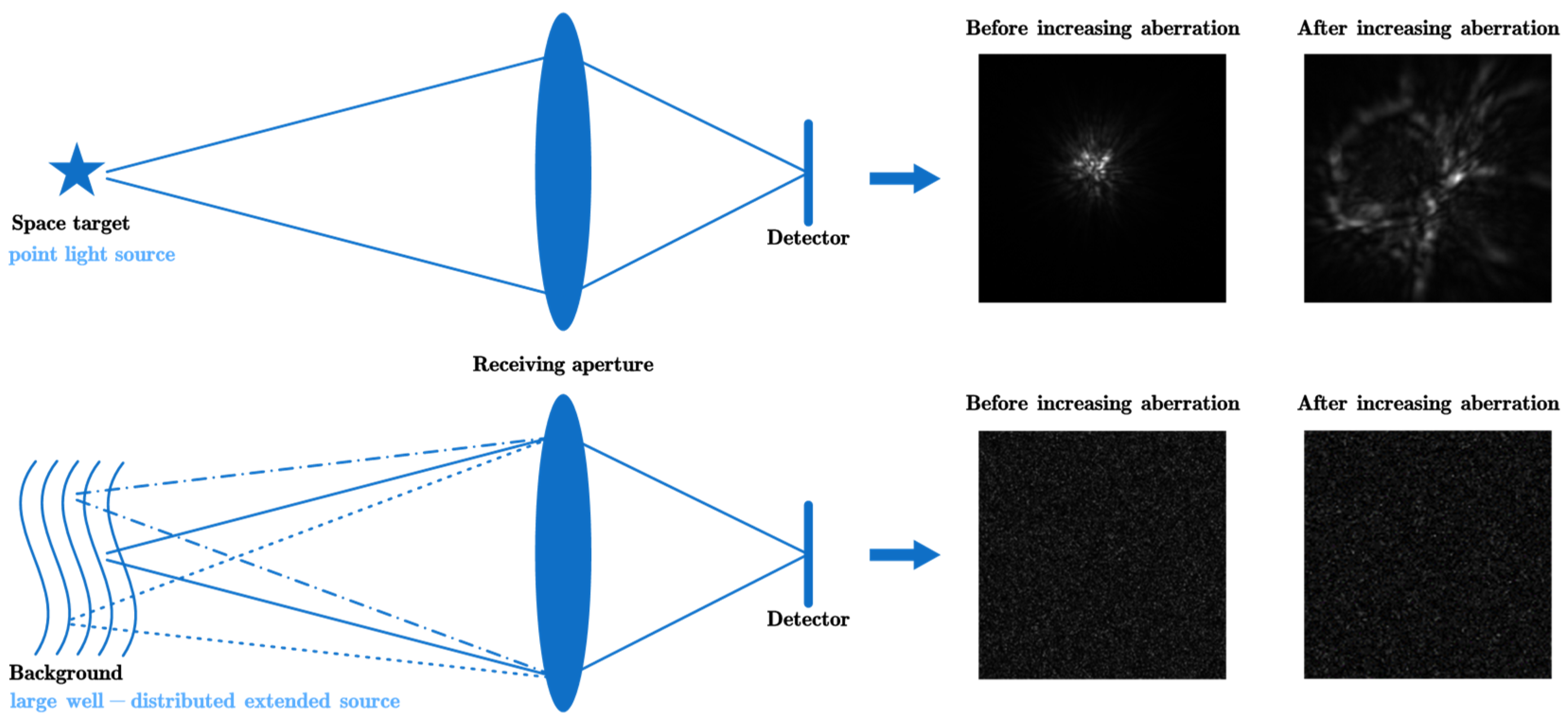
- To detect dim and small space targets, we proposed a target detection method based on aberration modulation and signal correlation (AMCM).
- (2)
- By performing active aberration modulation using the adaptive optics system and employing matched filtering for target-related detection, the feasibility and application potential of AMCM were preliminarily validated based on a self-constructed database and experiments.
- (3)
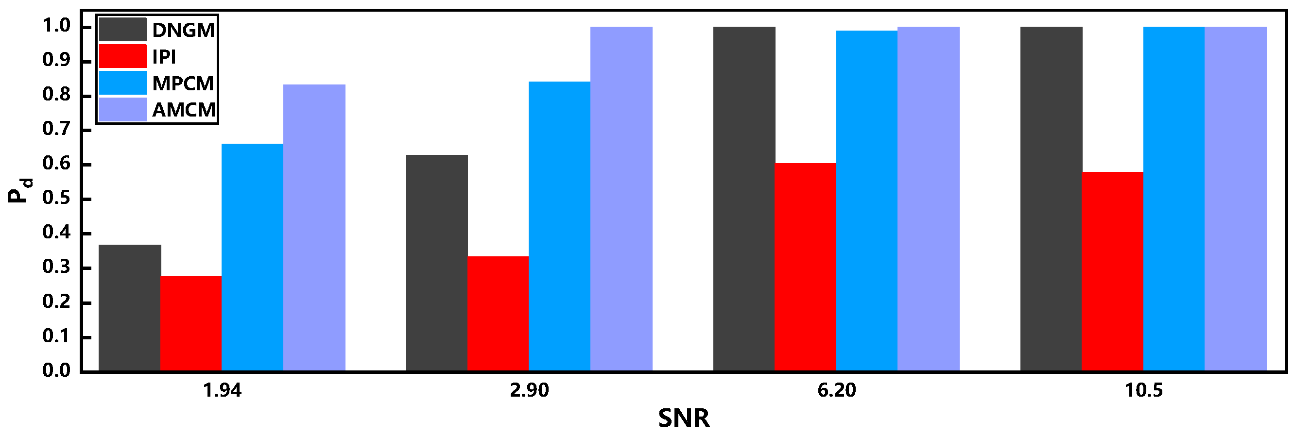
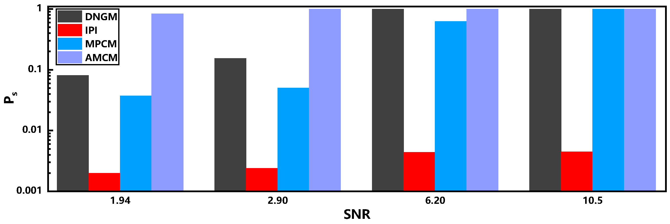
- Compared to traditional algorithm-based methods, AMCM achieved effective detection of targets with an SNR of 2, showing significant performance improvement.
2. Method
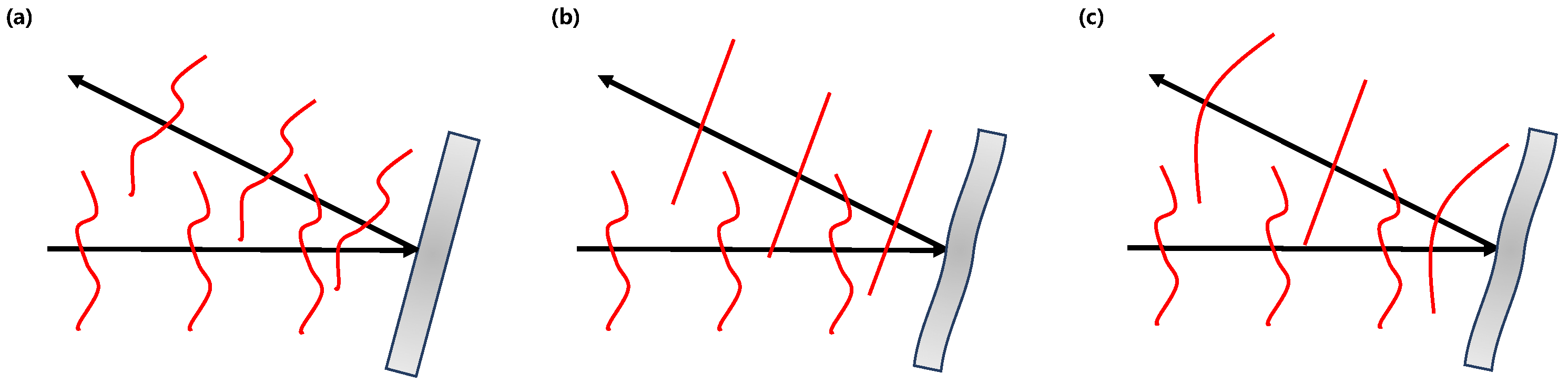
2.1. Principle
2.2. Process
2.3. Image Algorithm
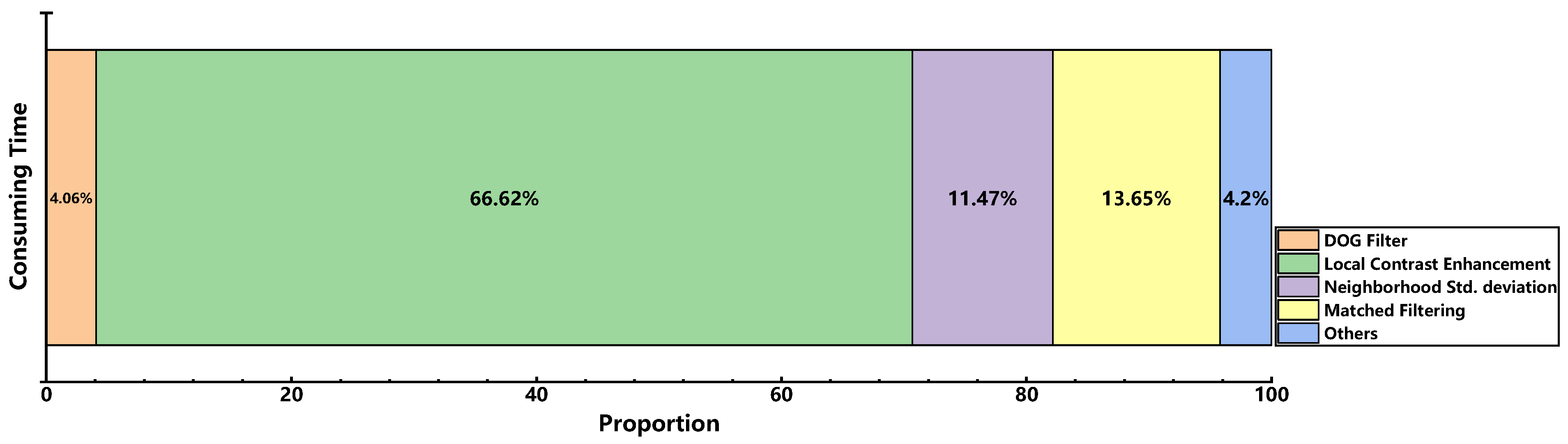
2.3.1. Pretreatment
- (1)
- DoG filter
- (2)
- Local contrast enhancement
- (3)
- Neighborhood Std. deviation
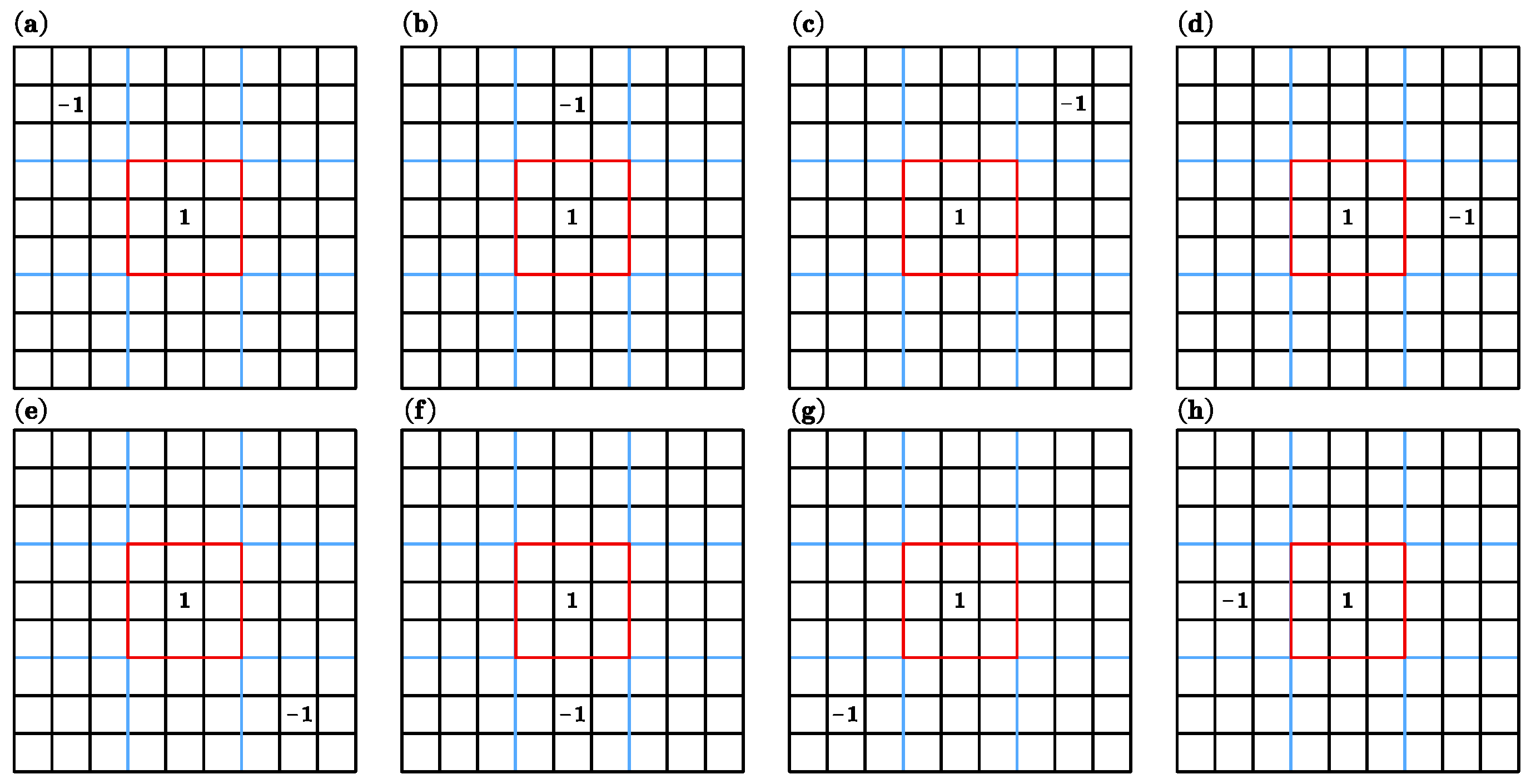
2.3.2. Matched Filtering
2.3.3. Post-Treatment
3. Results
3.1. Simulation
3.1.1. Data Generation
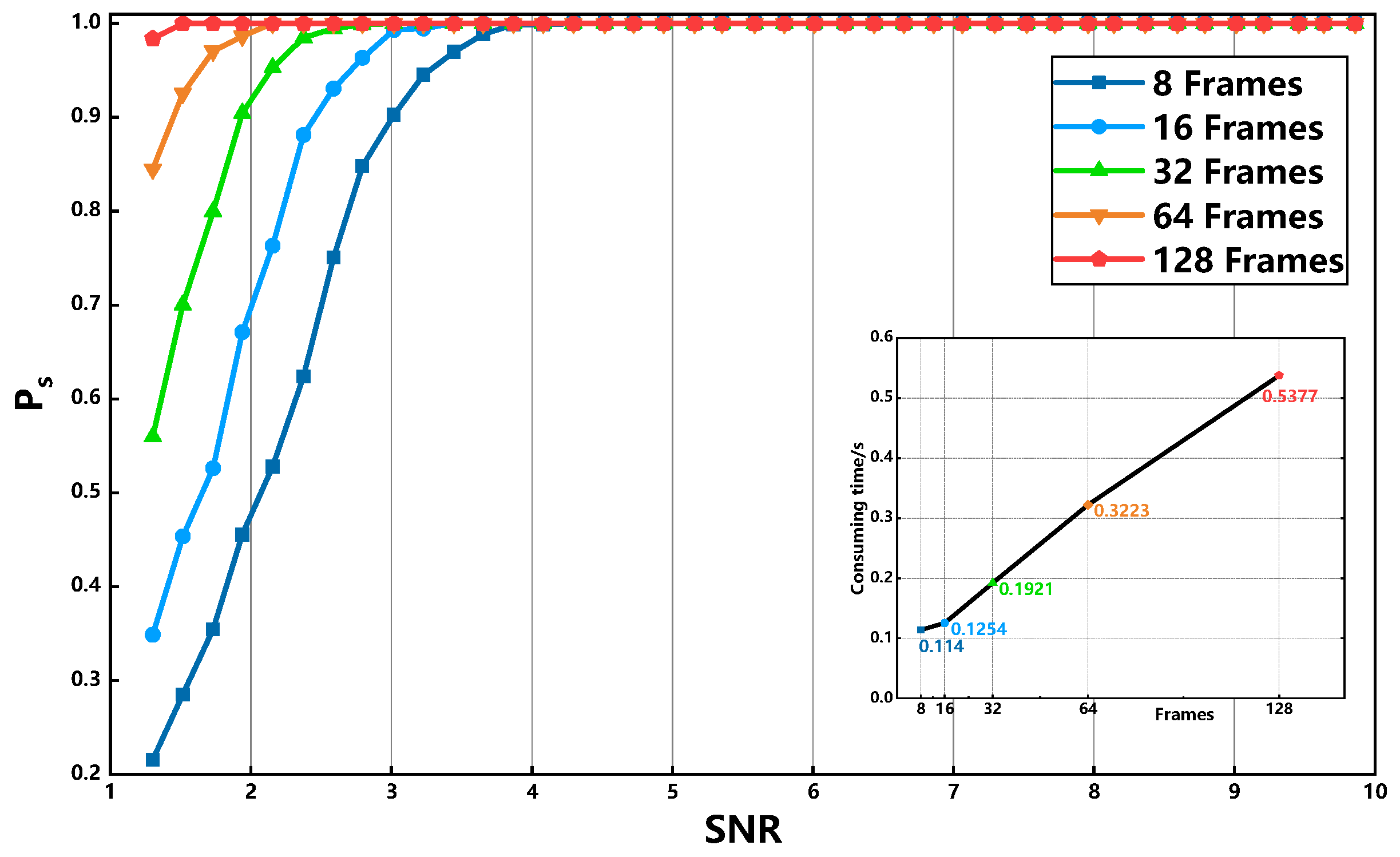
3.1.2. Sample Size
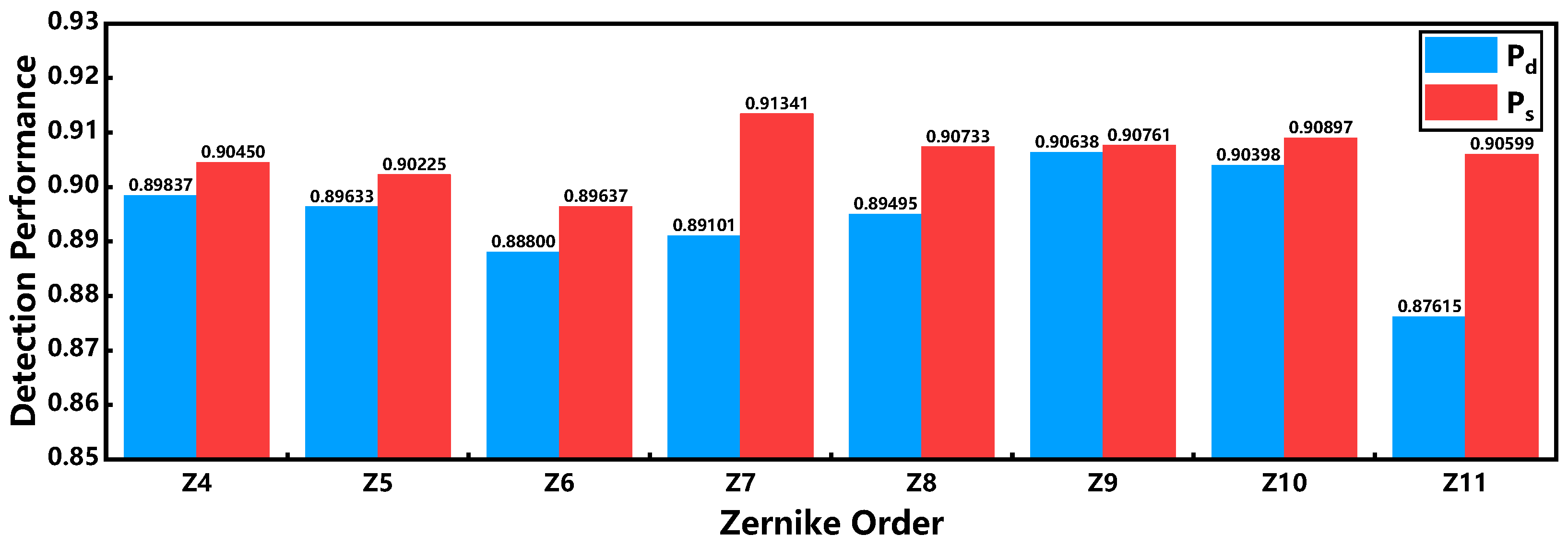
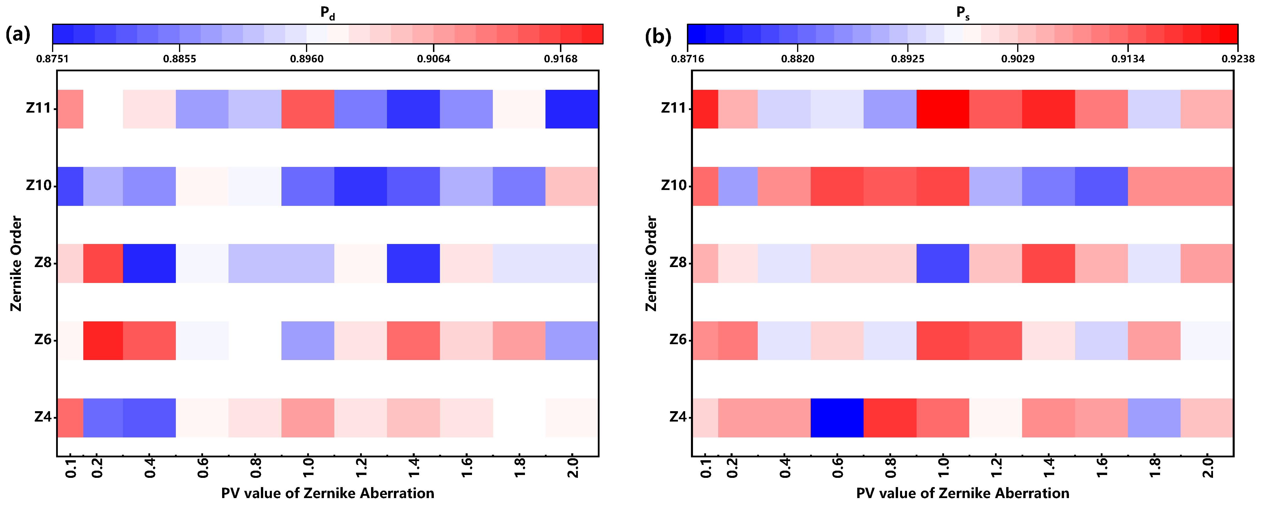
3.1.3. Aberration Type with Different PV Values
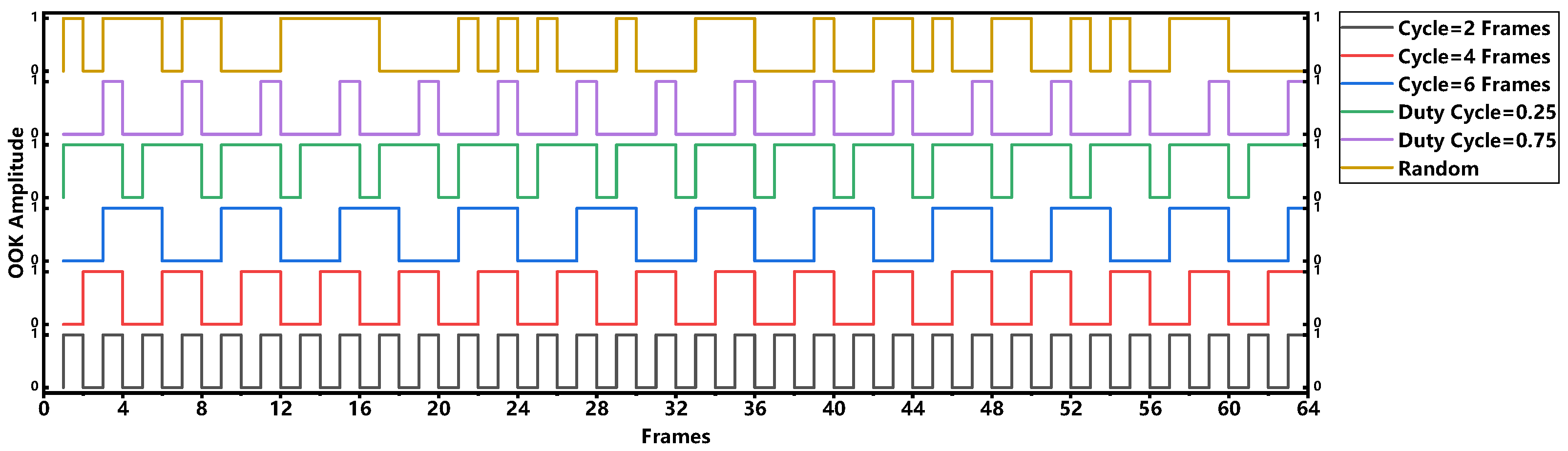
3.1.4. AMS
3.1.5. Classification Performance
3.1.6. Horizontal Comparison
3.2. Experiment
4. Discussion
4.1. Features and Applications of the Method
4.2. Factors Affecting Algorithms
4.3. Future Research Directions
4.3.1. Method Combination
4.3.2. Optical Simulation Computing Device
4.3.3. Moving Object Detection
4.3.4. Hyperparameter Search
Author Contributions
Funding
Data Availability Statement
Conflicts of Interest
References
- Leibovich, M.; Papanicolaou, G.; Tsogka, C. Generalized correlation-based imaging for satellites. SIAM J. Imaging Sci. 2020, 13, 1331–1366. [Google Scholar] [CrossRef]
- Woods, D.; Shah, R.; Johnson, J.; Pearce, E.; Lambour, R.; Faccenda, W. Asteroid detection with the space surveillance telescope. In Proceedings of the AMOS Conference, Maui, HI, USA, 10–13 September 2013. [Google Scholar]
- Zhao, M.; Li, W.; Li, L.; Hu, J.; Ma, P.; Tao, R. Single-Frame Infrared Small-Target Detection: A survey. IEEE Geosci. Remote Sens. Mag. 2022, 10, 87–119. [Google Scholar] [CrossRef]
- Nie, J.; Qu, S.; Wei, Y.; Zhang, L.; Deng, L. An infrared small target detection method based on multiscale local homogeneity measure. Infrared Phys. Technol. 2018, 90, 186–194. [Google Scholar] [CrossRef]
- Li, Y.; Zhang, Y. Robust infrared small target detection using local steering kernel reconstruction. Pattern Recognit. 2018, 77, 113–125. [Google Scholar] [CrossRef]
- Xia, C.; Li, X.; Zhao, L.; Yu, S. Modified graph Laplacian model with local contrast and consistency constraint for small target detection. IEEE J. Sel. Top. Appl. Earth Obs. Remote Sens. 2020, 13, 5807–5822. [Google Scholar] [CrossRef]
- Ren, X.; Yue, C.; Ma, T.; Wang, J.; Wang, J.; Wu, Y.; Weng, Z. Adaptive parameters optimization model with 3D information extraction for infrared small target detection based on particle swarm optimization algorithm. Infrared Phys. Technol. 2021, 117, 103838. [Google Scholar] [CrossRef]
- Zhou, D.; Wang, X. Research on high robust infrared small target detection method in complex background. IEEE Geosci. Remote Sens. Lett. 2023, 20, 6007705. [Google Scholar] [CrossRef]
- Lee, I.H.; Park, C.G. Infrared small target detection algorithm using an augmented intensity and density-based clustering. IEEE Trans. Geosci. Remote Sens. 2023, 61, 5002714. [Google Scholar] [CrossRef]
- Zhou, D.; Wang, X. Robust Infrared Small Target Detection Using a Novel Four-Leaf Model. IEEE J. Sel. Top. Appl. Earth Obs. Remote Sens. 2023, 17, 1462–1469. [Google Scholar] [CrossRef]
- Gao, C.; Meng, D.; Yang, Y.; Wang, Y.; Zhou, X.; Hauptmann, A.G. Infrared patch-image model for small target detection in a single image. IEEE Trans. Image Process. 2013, 22, 4996–5009. [Google Scholar] [CrossRef]
- Zhang, X.; Ding, Q.; Luo, H.; Hui, B.; Chang, Z.; Zhang, J. Infrared small target detection based on an image-patch tensor model. Infrared Phys. Technol. 2019, 99, 55–63. [Google Scholar] [CrossRef]
- Zhang, C.; He, Y.; Tang, Q.; Chen, Z.; Mu, T. Infrared small target detection via interpatch correlation enhancement and joint local visual saliency prior. IEEE Trans. Geosci. Remote Sens. 2021, 60, 5001314. [Google Scholar] [CrossRef]
- Dai, Y.; Wu, Y. Reweighted infrared patch-tensor model with both nonlocal and local priors for single-frame small target detection. IEEE J. Sel. Top. Appl. Earth Obs. Remote Sens. 2017, 10, 3752–3767. [Google Scholar] [CrossRef]
- Pang, D.; Shan, T.; Li, W.; Ma, P.; Tao, R.; Ma, Y. Facet derivative-based multidirectional edge awareness and spatial–temporal tensor model for infrared small target detection. IEEE Trans. Geosci. Remote Sens. 2021, 60, 5001015. [Google Scholar] [CrossRef]
- Li, Z.; Liao, S.; Wu, M.; Zhao, T.; Yu, H. Strengthened Local Feature-Based Spatial–Temporal Tensor Model for Infrared Dim and Small Target Detection. IEEE Sens. J. 2023, 23, 23221–23237. [Google Scholar] [CrossRef]
- Ju, M.; Luo, J.; Liu, G.; Luo, H. ISTDet: An efficient end-to-end neural network for infrared small target detection. Infrared Phys. Technol. 2021, 114, 103659. [Google Scholar] [CrossRef]
- Zhang, M.; Zhang, R.; Yang, Y.; Bai, H.; Zhang, J.; Guo, J. ISNet: Shape matters for infrared small target detection. In Proceedings of the IEEE/CVF Conference on Computer Vision. and Pattern Recognition, New Orleans, LA, USA, 18–24 June 2022; pp. 877–886. [Google Scholar] [CrossRef]
- Hou, Q.; Wang, Z.; Tan, F.; Zhao, Y.; Zheng, H.; Zhang, W. RISTDnet: Robust infrared small target detection network. IEEE Geosci. Remote Sens. Lett. 2021, 19, 7000805. [Google Scholar] [CrossRef]
- Yao, S.; Zhu, Q.; Zhang, T.; Cui, W.; Yan, P. Infrared image small-target detection based on improved FCOS and spatio-temporal features. Electronics 2022, 11, 933. [Google Scholar] [CrossRef]
- Wang, W.; Xiao, C.; Dou, H.; Liang, R.; Yuan, H.; Zhao, G.; Chen, Z.; Huang, Y. CCRANet: A Two-Stage Local Attention Network for Single-Frame Low-Resolution Infrared Small Target Detection. Remote Sens. 2023, 15, 5539. [Google Scholar] [CrossRef]
- Wang, H.; Zhou, L.; Wang, L. Miss detection vs. false alarm: Adversarial learning for small object segmentation in infrared images. In Proceedings of the IEEE/CVF International Conference on Computer Vision, Seoul, Republic of Korea, 27 October–2 November 2019; pp. 8509–8518. [Google Scholar] [CrossRef]
- Dai, Y.; Wu, Y.; Zhou, F.; Barnard, K. Asymmetric contextual modulation for infrared small target detection. In Proceedings of the IEEE/CVF Winter Conference on Applications of Computer Vision, Virtual, 5–9 January 2021; pp. 950–959. [Google Scholar] [CrossRef]
- Dai, Y.; Li, X.; Zhou, F.; Qian, Y.; Chen, Y.; Yang, J. One-stage cascade refinement networks for infrared small target detection. IEEE Trans. Geosci. Remote Sens. 2023, 61, 5000917. [Google Scholar] [CrossRef]
- Conforti, G. Zernike aberration coefficients from Seidel and higher-order power-series coefficients. Opt. Lett. 1983, 8, 407–408. [Google Scholar] [CrossRef] [PubMed]
- Milanfar, P. Two-dimensional matched filtering for motion estimation. IEEE Trans. Image Process 2002, 8, 438–444. [Google Scholar] [CrossRef] [PubMed]
- Kenneth, R. Castleman, Digital Image Processing; Prentice Hall Press: Saddle River, NJ, USA, 1996. [Google Scholar]
- Wei, Y.; You, X.; Li, H. Multiscale patch-based contrast measure for small infrared target detection. Pattern Recognit. 2016, 58, 216–226. [Google Scholar] [CrossRef]
- Koz, A.; Alatan, A.A. Oblivious Spatio-Temporal Watermarking of Digital Video by Exploiting the Human Visual System. IEEE Trans. Circuits Syst. Video Technol. 2008, 18, 326–337. [Google Scholar] [CrossRef]
- Kim, S.; Lee, J. Scale invariant small target detection by optimizing signal-to-clutter ratio in heterogeneous background for infrared search and track. Pattern Recognit. 2012, 45, 393–406. [Google Scholar] [CrossRef]
- Wang, C.; Luo, M.; Su, X.; Lan, X.; Sun, Z.; Gao, J.; Ye, M.; Zhu, J. A sliding-window based signal processing method for characterizing particle clusters in gas-solids high-density CFB reactor. Chem. Eng. J. 2023, 452, 139141. [Google Scholar] [CrossRef]
- Sortino, M. Application of Statistical Filtering for Optical Detection of Tool Wear. Int. J. Mach. Tools Manuf. 2003, 43, 493–497. [Google Scholar] [CrossRef]
- Qin, T.; Mu, G.; Zhao, P.; Tan, Y.; Liu, Y.; Zhang, S.; Luo, Y.; Hao, Q.; Chen, M.; Tang, X. Mercury telluride colloidal quantum-dot focal plane array with planar p-n junctions enabled by in situ electric field–activated doping. Sci. Adv. 2023, 9, eadg7827. [Google Scholar] [CrossRef]
- Dudzik, M.C. Electro-Optical Systems Design, Analysis, and Testing. In The Infrared and Electro-Optical Systems Handbook; Environment Research Institute of Michigan & SPIE: Ann Arbor, MI, USA, 1993; Volume 4. [Google Scholar]
- Guo, Y.; Chen, K.; Zhou, J.; Li, Z.; Han, W.; Rao, X.; Bao, H.; Yang, J.; Fan, X.; Rao, C. High-resolution visible imaging with piezoelectric deformable secondary mirror: Experimental results at the 1.8-m adaptive telescope. Opto-Electron. Adv. 2023, 6, 230039-1. [Google Scholar] [CrossRef]
- Isautier, P.; Pan, J.; DeSalvo, R.; Ralph, S.E. Stokes Space-Based Modulation Format Recognition for Autonomous Optical Receivers. J. Light. Technol. 2015, 33, 5157–5163. [Google Scholar] [CrossRef]
- Cook, J.; Ramadas, V. When to consult precision-recall curves. Stata J. 2020, 20, 131–148. [Google Scholar] [CrossRef]
- Wu, L.; Ma, Y.; Fan, F.; Wu, M.; Huang, J. A Double-Neighborhood Gradient Method for Infrared Small Target Detection. IEEE Geosci. Remote Sens. Lett. 2020, 18, 1476–1480. [Google Scholar] [CrossRef]
- Liu, K.; Zhang, Y.; Gao, T.; Tong, F.; Liu, P.; Li, W.; Li, M. A handheld rapid detector of soil total nitrogen based on phase-locked amplification technology. Comput. Electron. Agric. 2024, 224, 109233. [Google Scholar] [CrossRef]
- Cheng, J.; Xu, Y.; Wu, L.; Wang, G. A Digital Lock-In Amplifier for Use at Temperatures of up to 200 °C. Sensors 2016, 16, 1899. [Google Scholar] [CrossRef] [PubMed]
- Enz, C.C.; Temes, G.C. Circuit Techniques for Reducing the Effects of Op-Amp Imperfections: Autozeroing, Correlated Double Sampling, and Chopper Stabilization. Proc. IEEE 1996, 84, 1584–1614. [Google Scholar] [CrossRef]
- Tanriover, I.; Dereshgi, S.A.; Aydin, K. Metasurface enabled broadband all optical edge detection in visible frequencies. Nat. Commun. 2023, 14, 6484. [Google Scholar] [CrossRef]
- Bustio-Martínez, L.; Cumplido, R.; Letras, M.; Hernández-León, R.; Feregrino-Uribe, C.; Hernández-Palancar, J. FPGA/GPU-based Acceleration for Frequent Itemsets Mining: A Comprehensive Review. ACM Comput. Surv. 2021, 54, 179. [Google Scholar] [CrossRef]
- Chen, C.L.P.; Li, H.; Wei, Y.; Xia, T.; Tang, Y.Y. A Local Contrast Method for Small Infrared Target Detection. IEEE Trans. Geosci. Remote Sens. 2014, 52, 574–581. [Google Scholar] [CrossRef]
- Han, J.; Ma, Y.; Zhou, B.; Fan, F.; Liang, K.; Fang, Y. A Robust Infrared Small Target Detection Algorithm Based on Human Visual System. IEEE Geosci. Remote Sens. Lett. 2014, 11, 2168–2172. [Google Scholar] [CrossRef]
- Xie, K.; Fu, K.; Zhou, T.; Zhang, J.; Yang, J.; Wu, Q. Small target detection based on accumulated center-surround difference measure. Infrared Phys. Technol. 2014, 67, 229–236. [Google Scholar] [CrossRef]
- Ren, X.; Wang, J.; Ma, T.; Bai, K.; Ge, M.; Wang, Y. Infrared dim and small target detection based on three-dimensional collaborative filtering and spatial inversion modeling. Infrared Phys. Technol. 2019, 101, 13–24. [Google Scholar] [CrossRef]
- Genin, L.; Champagnat, F.; Le Besnerais, G.; Coret, L. Point object detection using a NL-means type filter. In Proceedings of the 2011 18th IEEE International Conference on Image Processing, Brussels, Belgium, 11–14 September 2011; pp. 3533–3536. [Google Scholar] [CrossRef]
- Abdeldayem, H.; Frazier, D.O. Optical computing. Commun. ACM 2007, 50, 60–62. [Google Scholar] [CrossRef]
- Zhou, Y.; Zheng, H.; Kravchenko, I.I.; Valentine, J. Flat optics for image differentiation. Nat. Photonics 2020, 14, 316–323. [Google Scholar] [CrossRef]
- Xu, Y.; Huang, L.; Jiang, W.; Guan, X.; Hu, W.; Yi, L. End-to-End Learning for 100G-PON Based on Noise Adaptation Network. J. Light. Technol. 2024, 42, 2328–2337. [Google Scholar] [CrossRef]
- Qiang, Y.; Jiao, L.C.; Bao, Z. Study on mechanism of dynamic programming algorithm for dim target detection. In Proceedings of the 6th International Conference on Signal Processing, Beijing, China, 26–30 August 2002; Volume 2, pp. 1403–1406. [Google Scholar]
- Liou, R.J.; Azimi-Sadjadi, M.R. Dim target detection using high order correlation method. IEEE Trans. Aerosp. Electron. Syst. 1993, 29, 841–856. [Google Scholar] [CrossRef]
- Jin, D.; Lei, J.; Peng, B.; Li, W.; Ling, N.; Huang, Q. Deep Affine Motion Compensation Network for Inter Prediction in VVC. IEEE Trans. Circuits Syst. Video Technol. 2022, 32, 3923–3933. [Google Scholar] [CrossRef]
- Tang, K.; Astola, J.; Neuvo, Y. Nonlinear multivariate image filtering techniques. IEEE Trans. Image Process 1995, 4, 788–798. [Google Scholar] [CrossRef]
- Lancaster, J.; Lorenz, R.; Leech, R.; Cole, J.H. Bayesian Optimization for Neuroimaging Pre-processing in Brain Age Classification and Prediction. Front. Aging Neurosci. 2018, 10, 28. [Google Scholar] [CrossRef]
- Thangaraj, R.; Pant, M.; Abraham, A.; Bouvry, P. Particle swarm optimization: Hybridization perspectives and experimental illustrations. Appl. Math. Comput. 2011, 217, 5208–5226. [Google Scholar] [CrossRef]
- Ji, J.; Song, S.; Tang, C.; Gao, S.; Tang, Z.; Todo, Y. An artificial bee colony algorithm search guided by scale-free networks. Inf. Sci. 2019, 473, 142–165. [Google Scholar] [CrossRef]


Disclaimer/Publisher’s Note: The statements, opinions and data contained in all publications are solely those of the individual author(s) and contributor(s) and not of MDPI and/or the editor(s). MDPI and/or the editor(s) disclaim responsibility for any injury to people or property resulting from any ideas, methods, instructions or products referred to in the content. |
© 2024 by the authors. Licensee MDPI, Basel, Switzerland. This article is an open access article distributed under the terms and conditions of the Creative Commons Attribution (CC BY) license (https://creativecommons.org/licenses/by/4.0/).
Share and Cite
Jiang, C.; Li, J.; Liu, S.; Xian, H. Aberration Modulation Correlation Method for Dim and Small Space Target Detection. Remote Sens. 2024, 16, 3729. https://doi.org/10.3390/rs16193729
Jiang C, Li J, Liu S, Xian H. Aberration Modulation Correlation Method for Dim and Small Space Target Detection. Remote Sensing. 2024; 16(19):3729. https://doi.org/10.3390/rs16193729
Chicago/Turabian StyleJiang, Changchun, Junwei Li, Shengjie Liu, and Hao Xian. 2024. "Aberration Modulation Correlation Method for Dim and Small Space Target Detection" Remote Sensing 16, no. 19: 3729. https://doi.org/10.3390/rs16193729