


Evaluating Ecological Drought Vulnerability from Ecosystem Service Value Perspectives in North China

 ,
,
Abstract
:1. Introduction
2. Materials
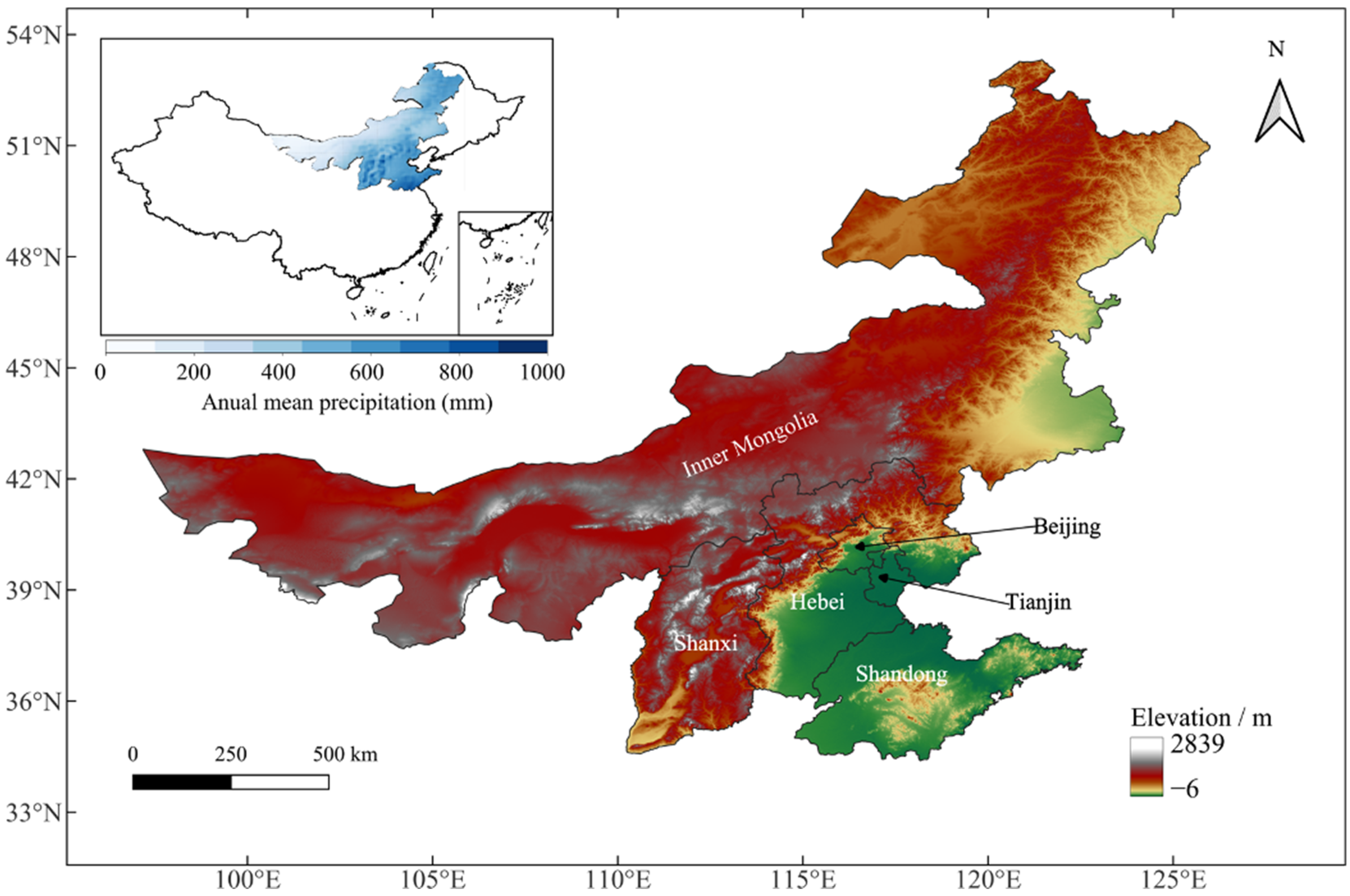
2.1. Study Region
2.2. Dataset
3. Method
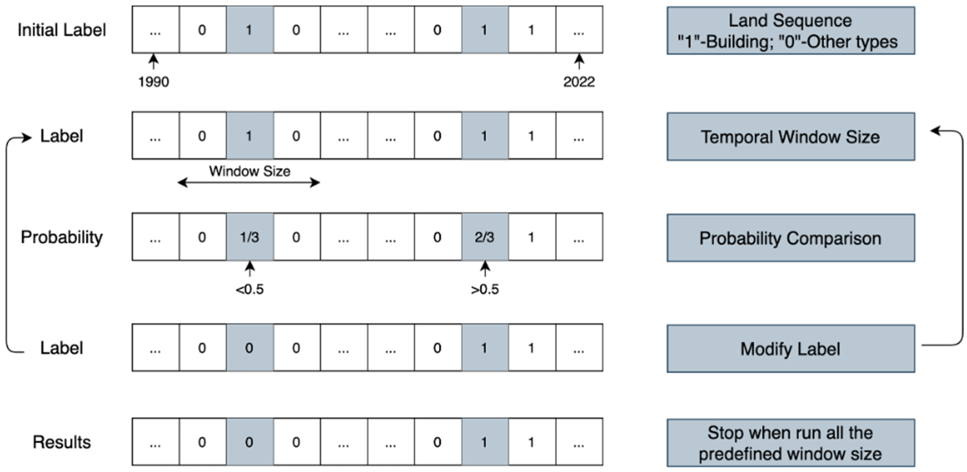
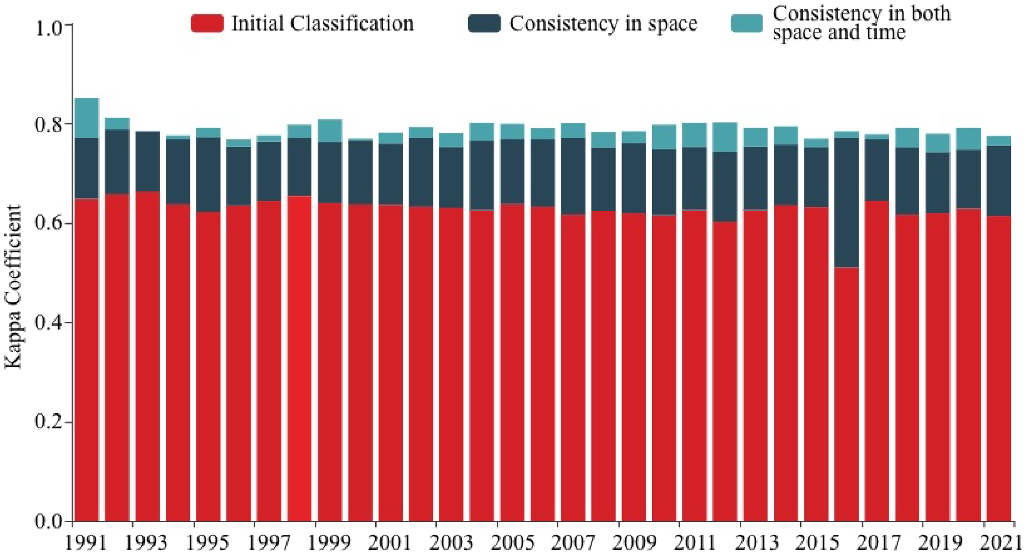
3.1. Optimizing Land Use Classification Based on Google Earth Engine
3.2. Constructing Ecosystem Service Value Dynamic Assessment Methods Based on Google Earth Engine
3.3. Constructing Ecological Drought Index
3.3.1. Ecological Water Deficit
3.3.2. Standardized Ecological Water Deficit Index
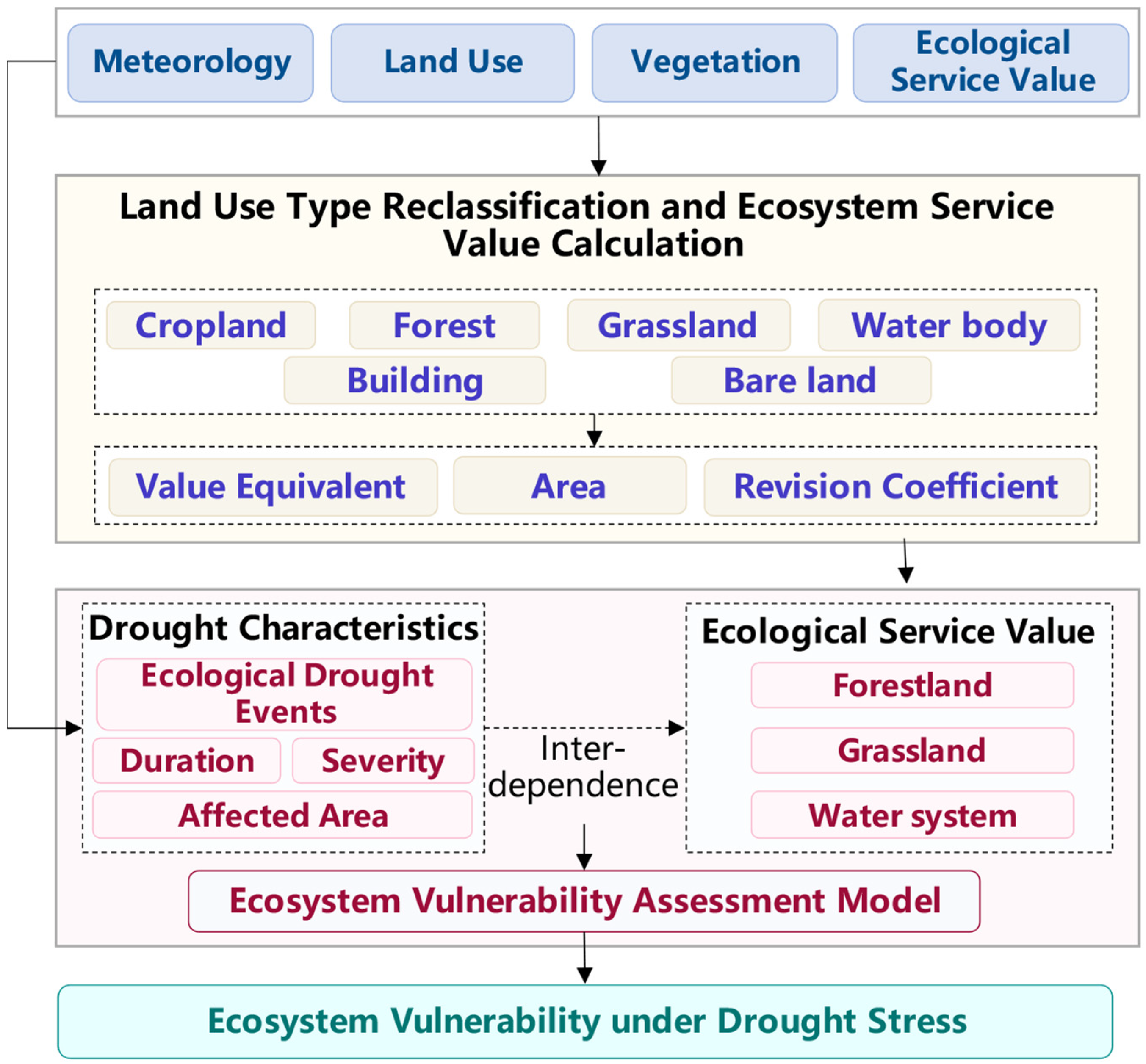
3.4. Vulnerability Assessment of Ecosystems
4. Results
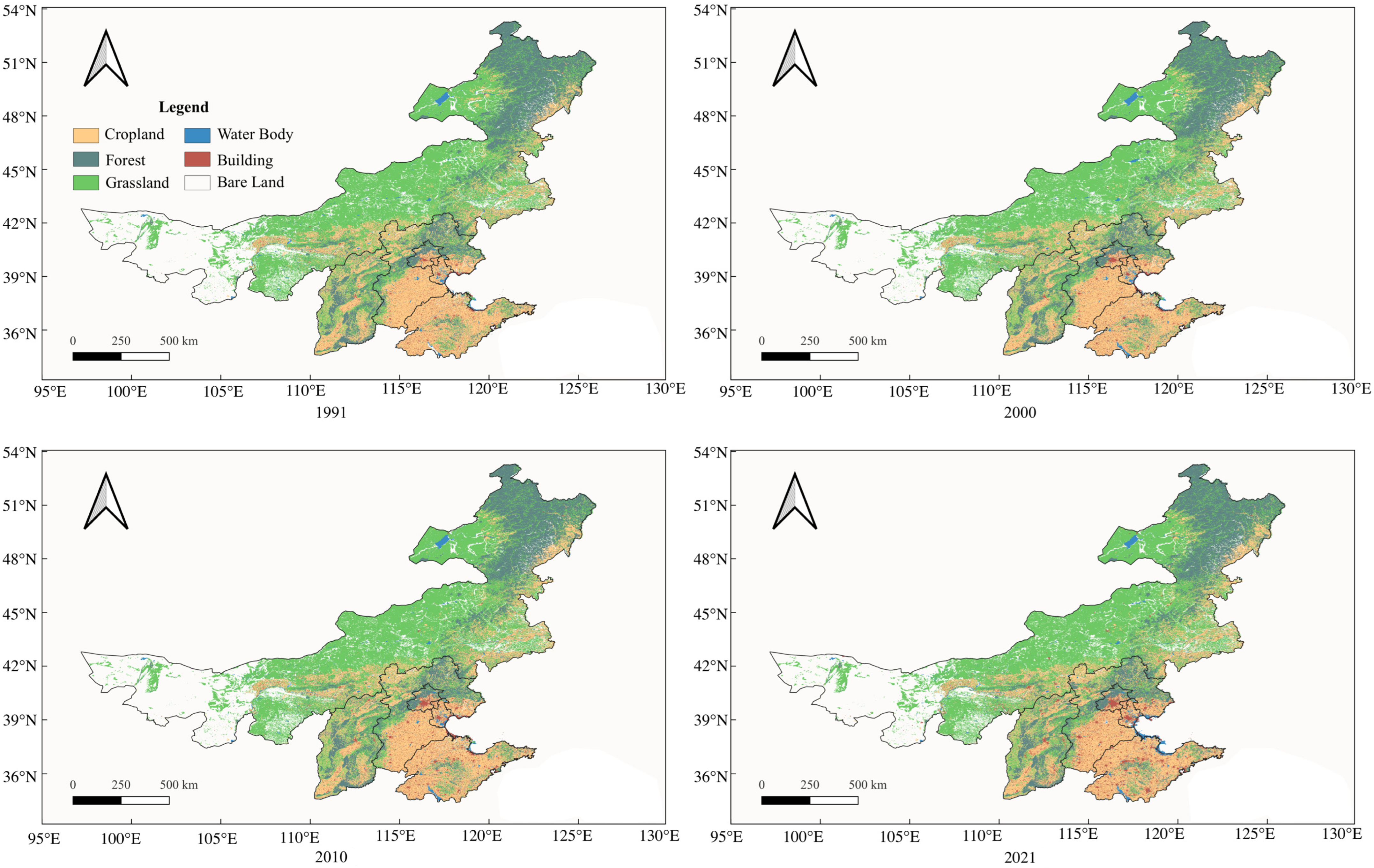
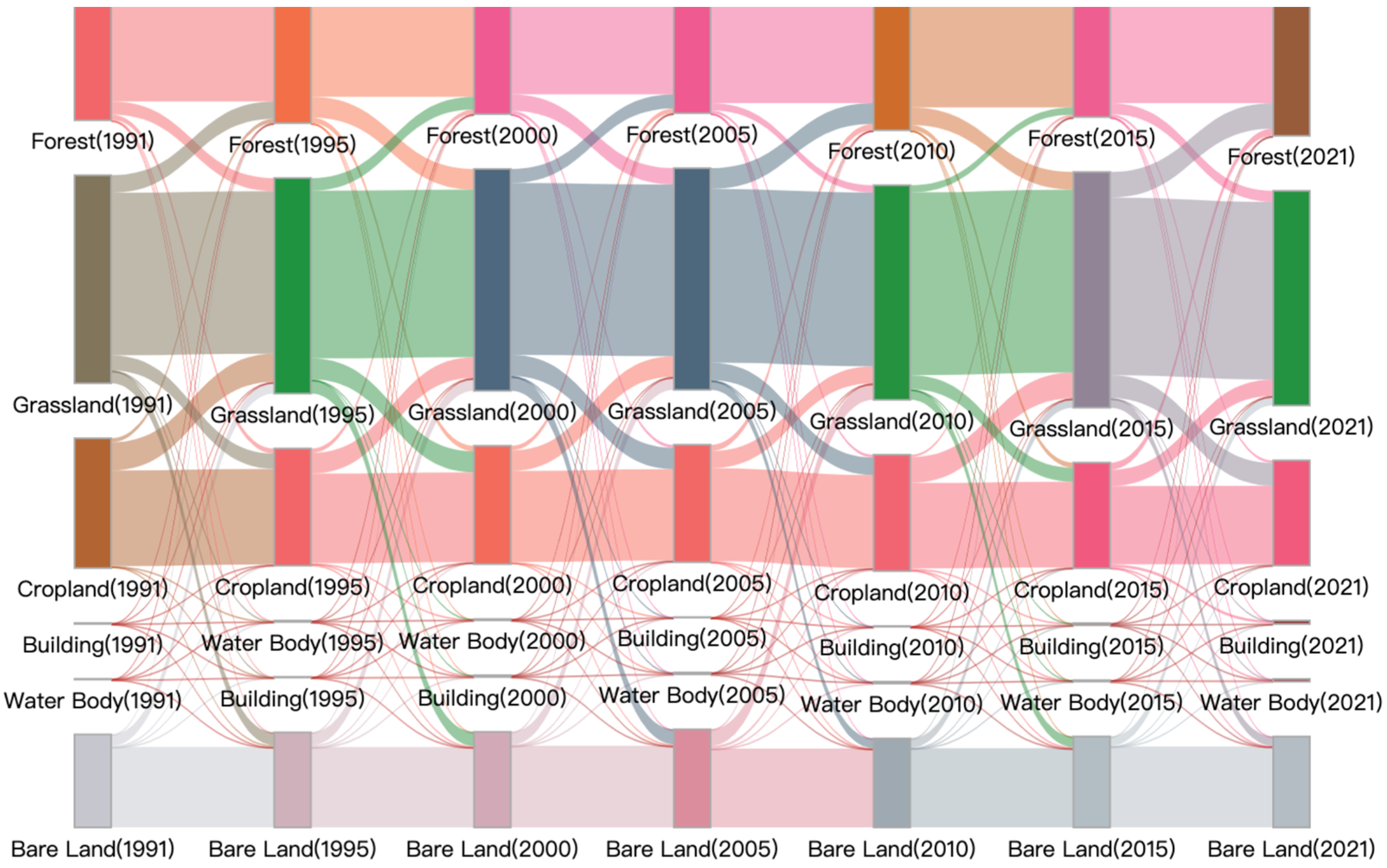
4.1. Land Use Change in North China
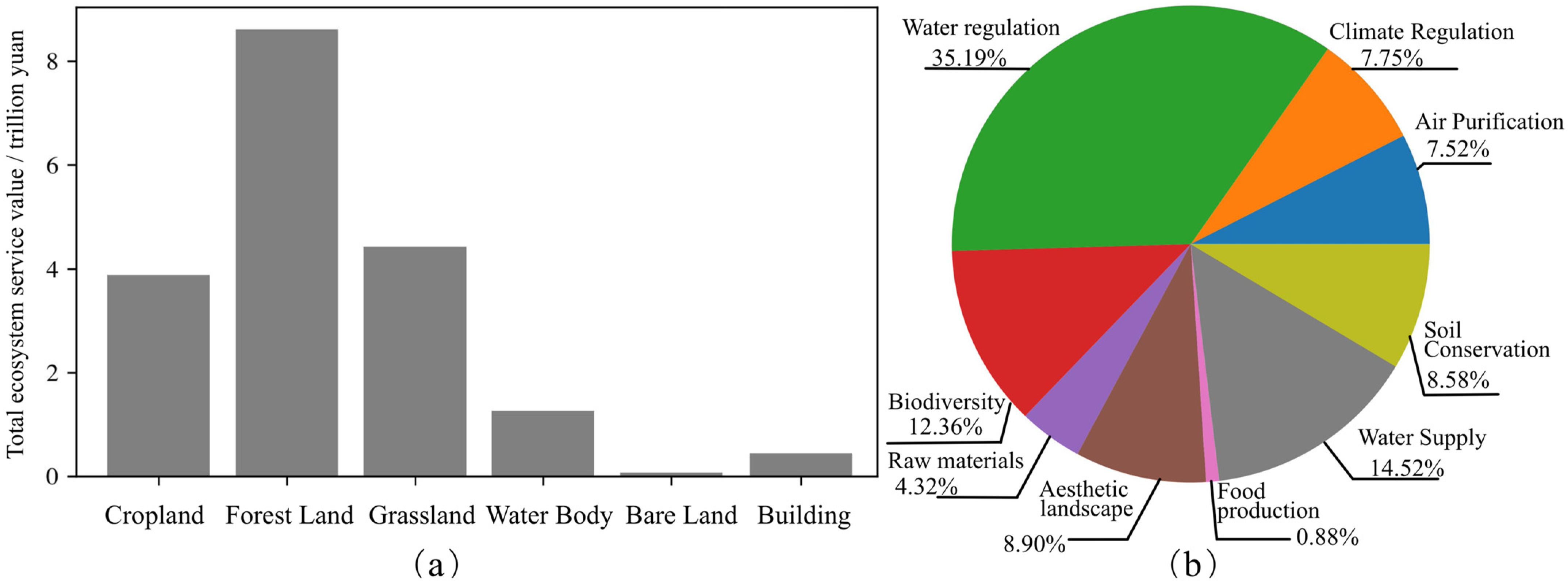
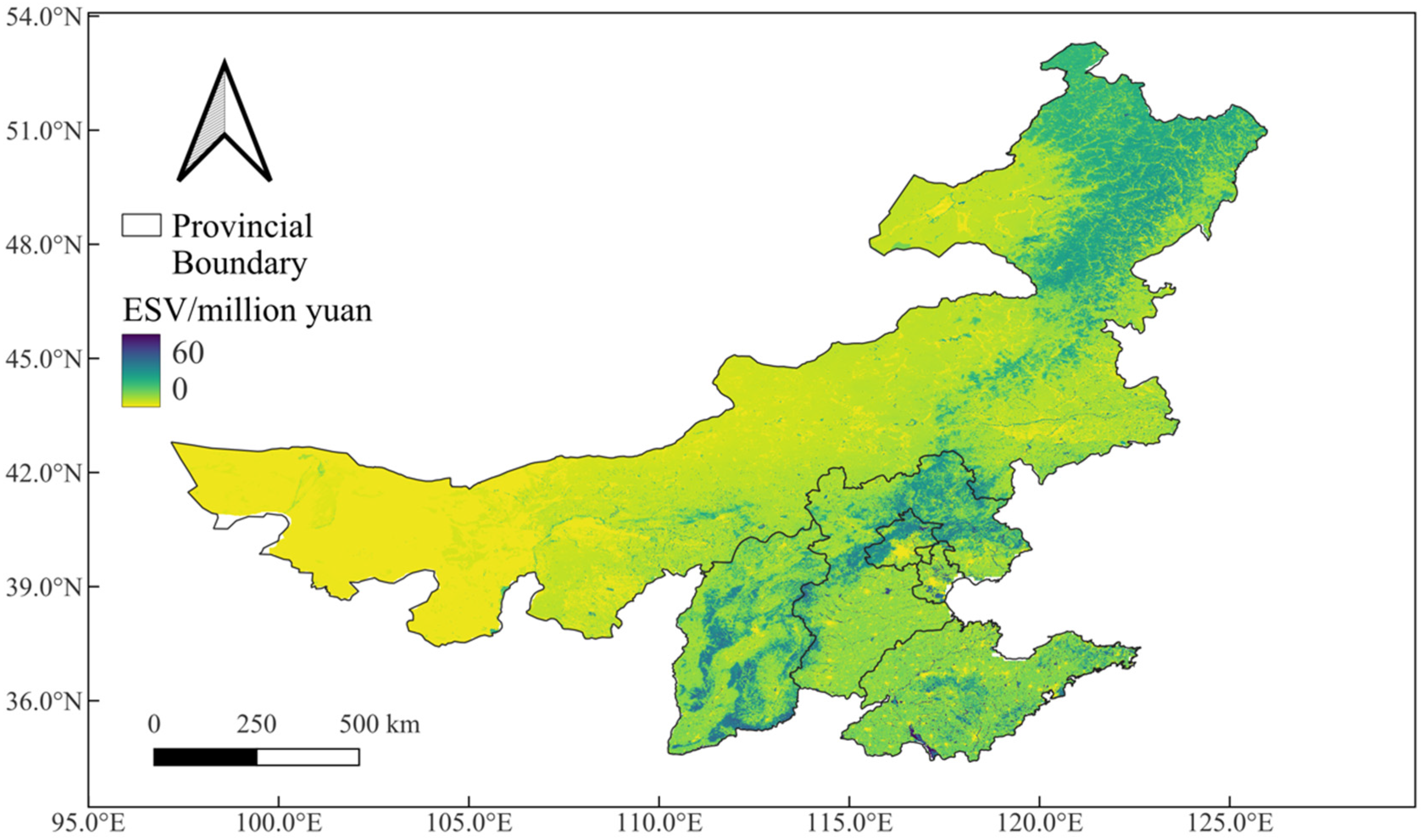
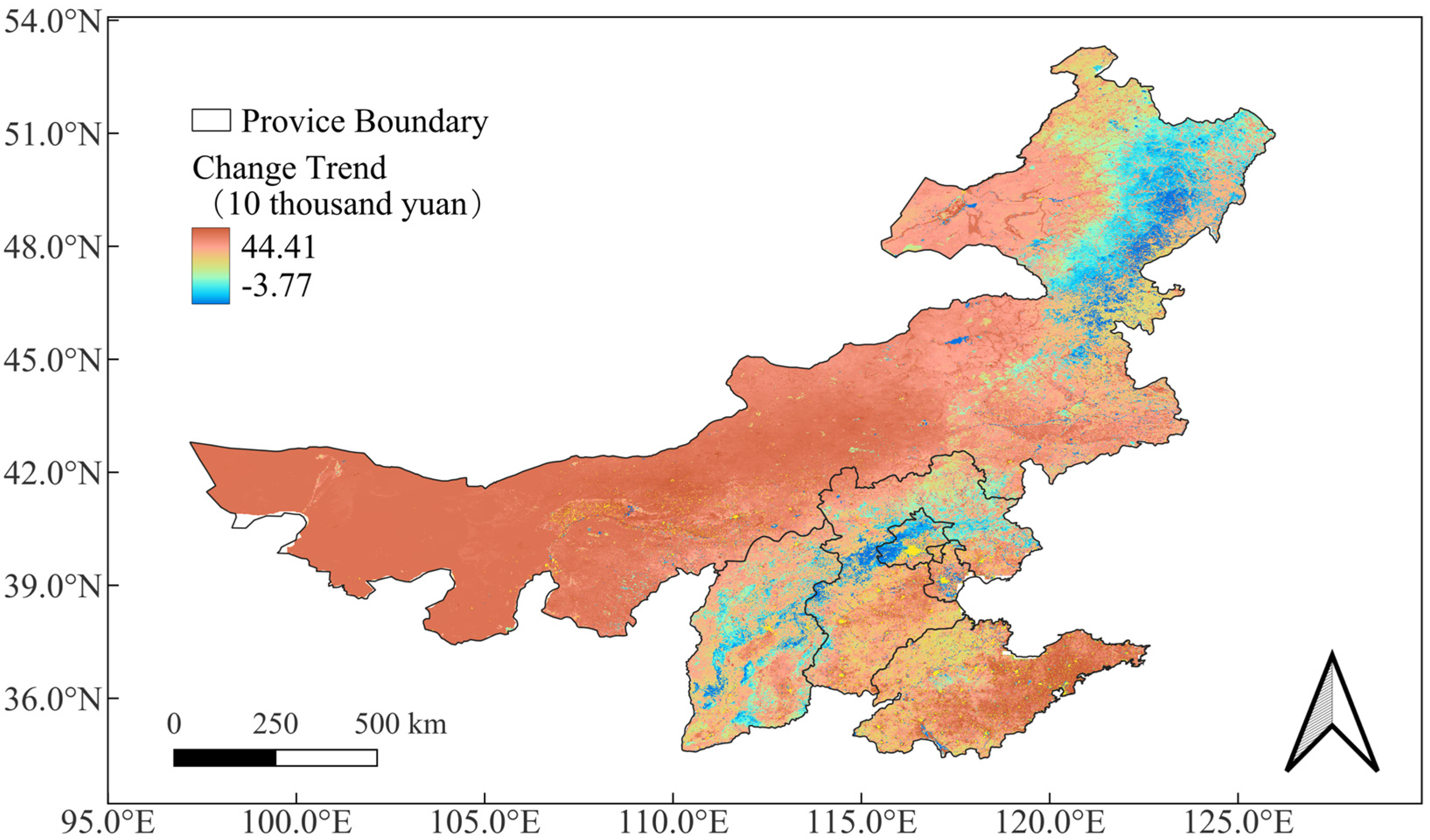
4.2. Spatiotemporal Dynamics of Ecosystem Service Values in North China
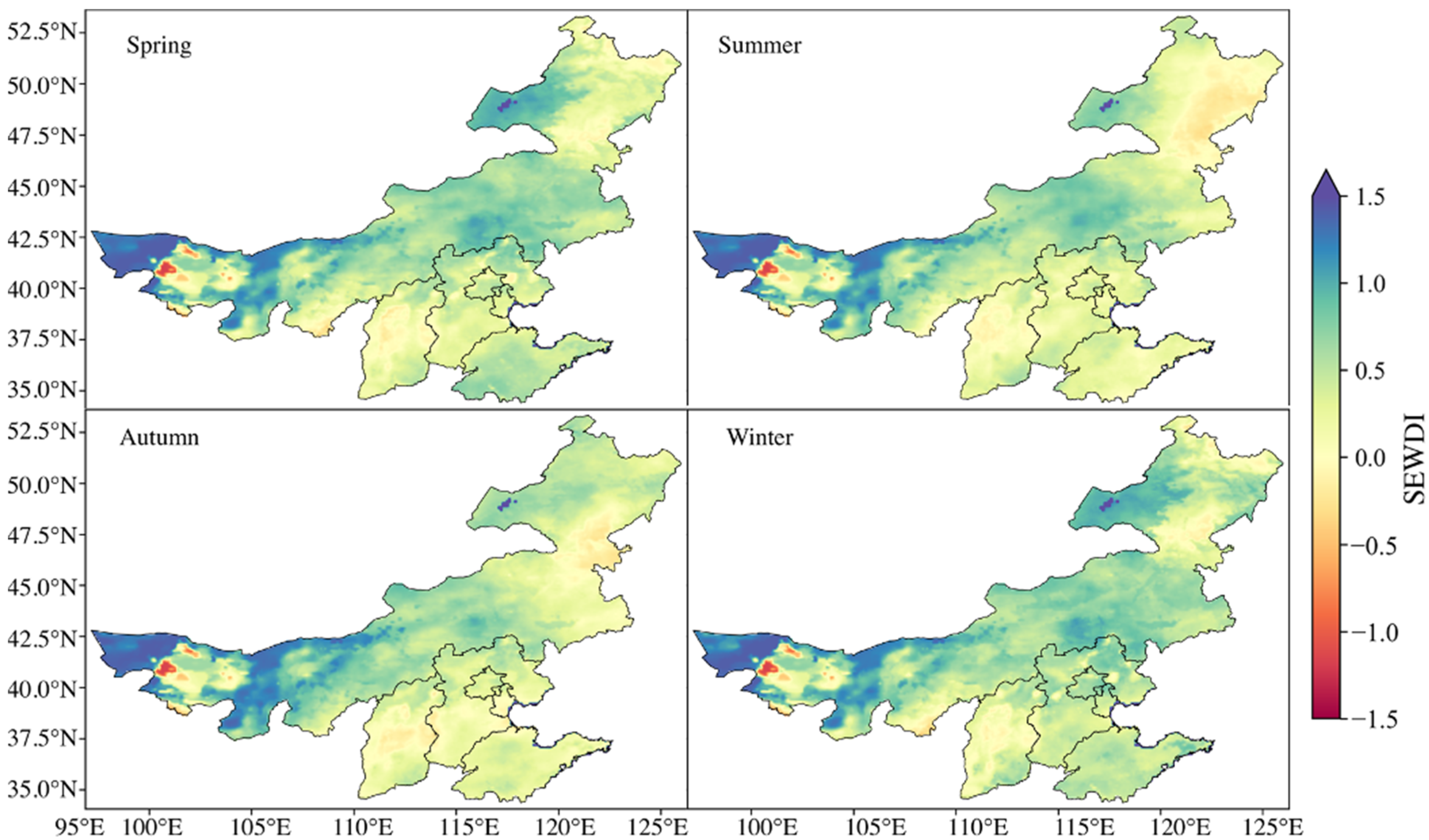
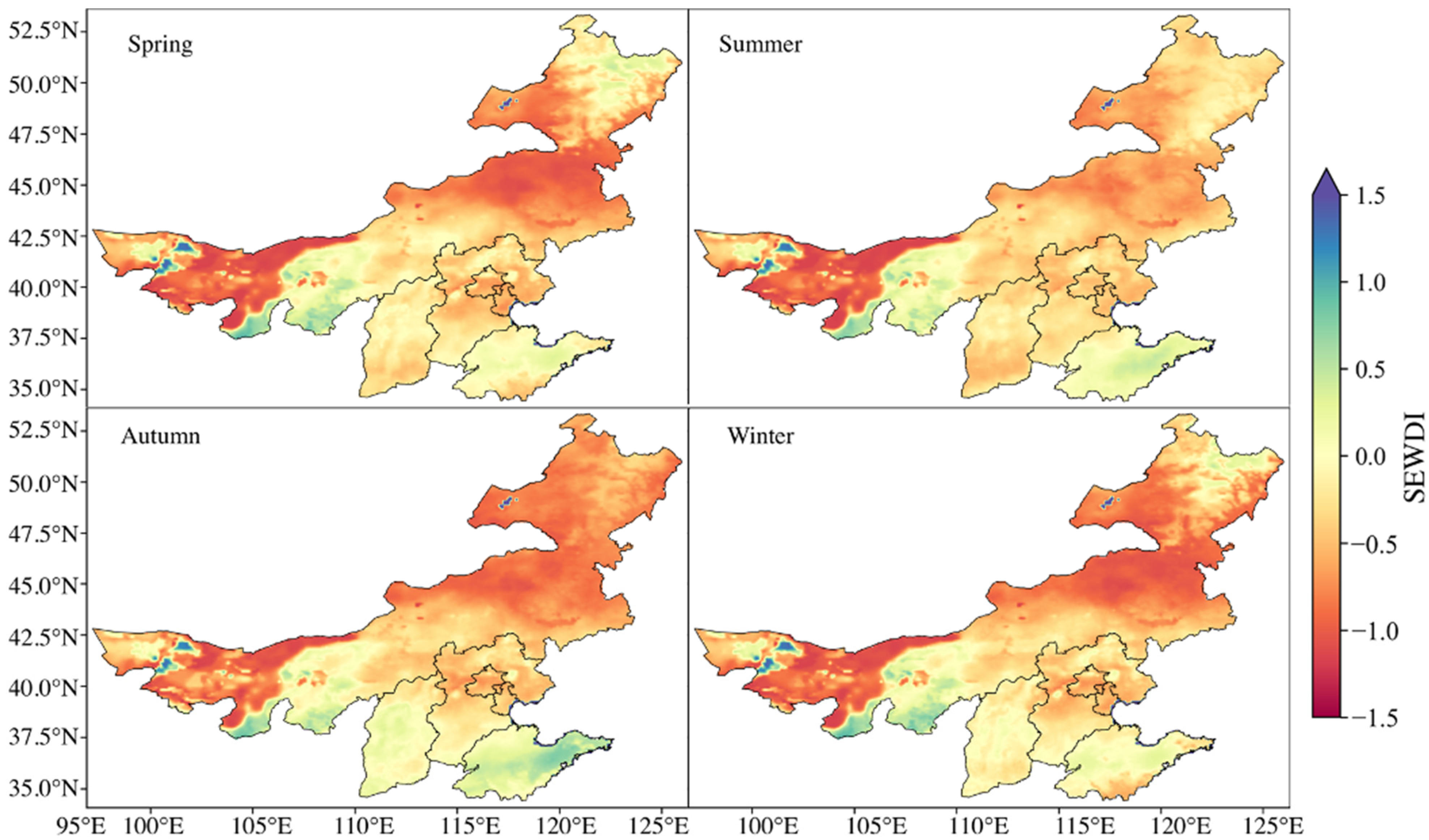
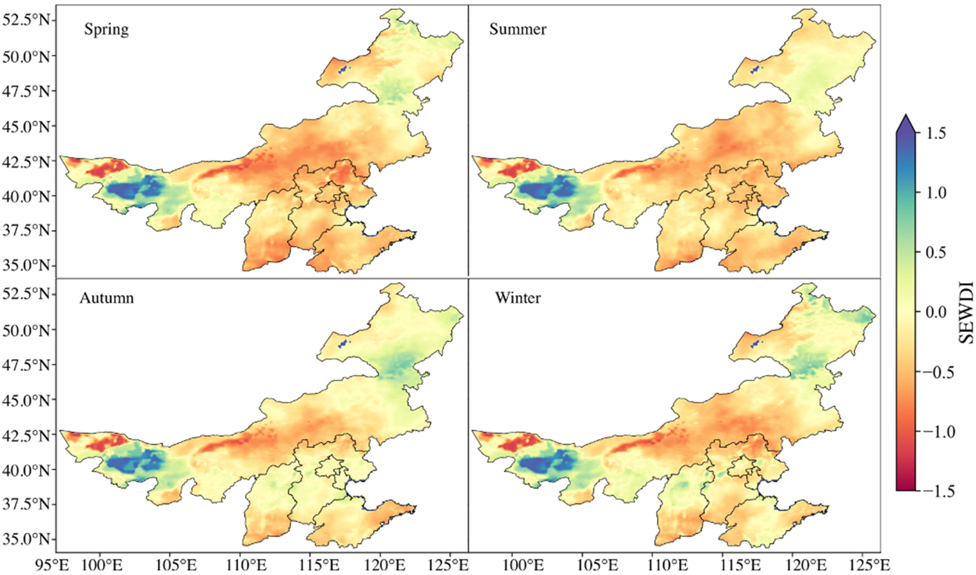
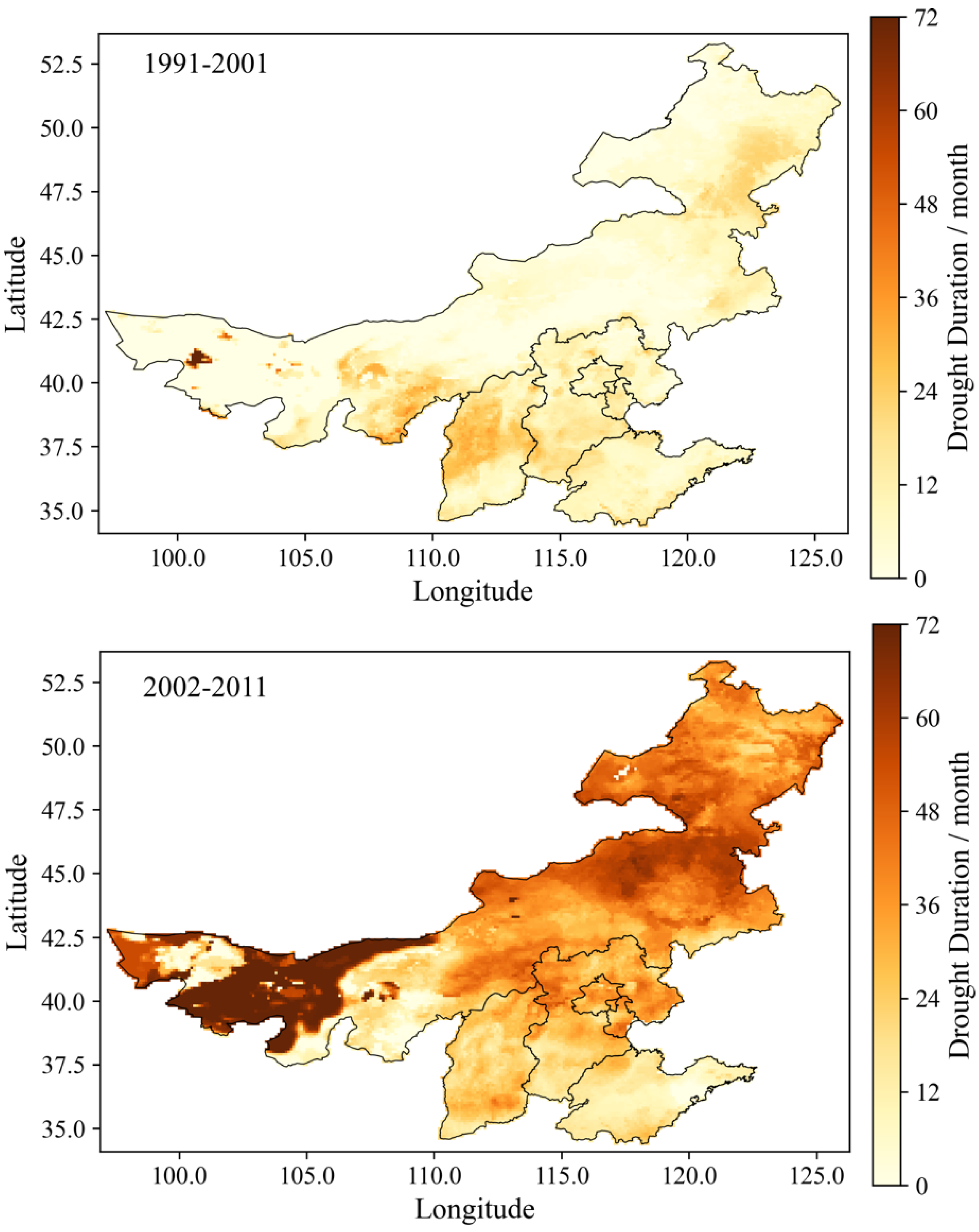
4.3. Spatiotemporal Variation of Ecological Drought
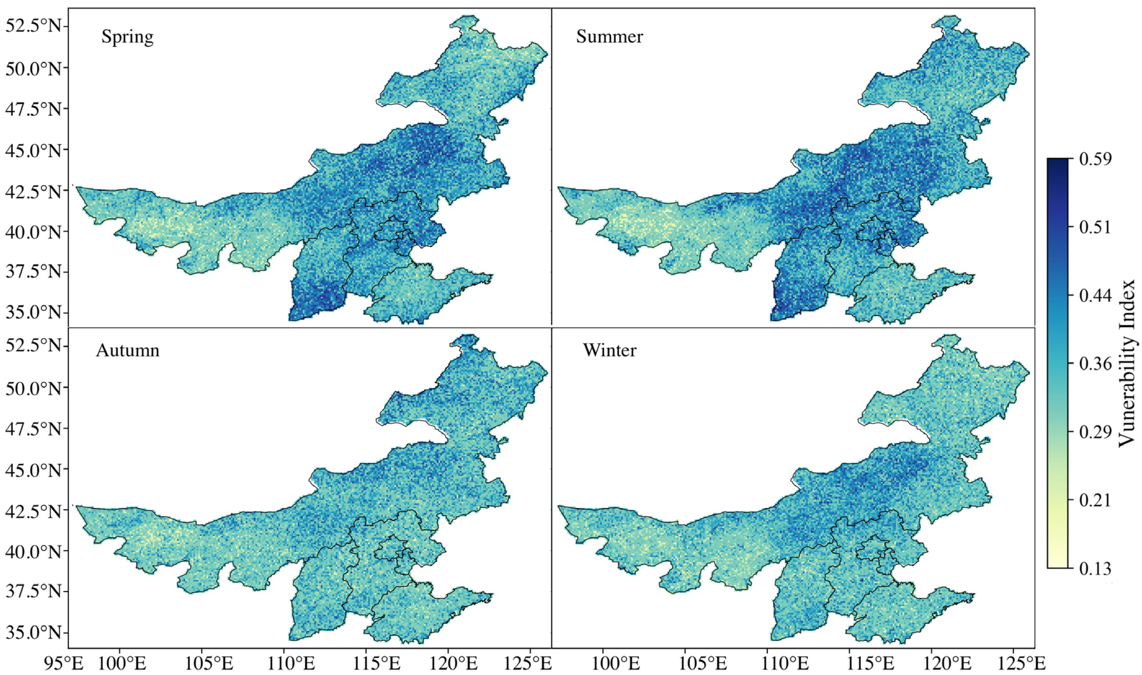
4.4. Ecosystem Vulnerability Assessment
5. Discussion
5.1. Ecological Drought and Its Impact on ESV in North China
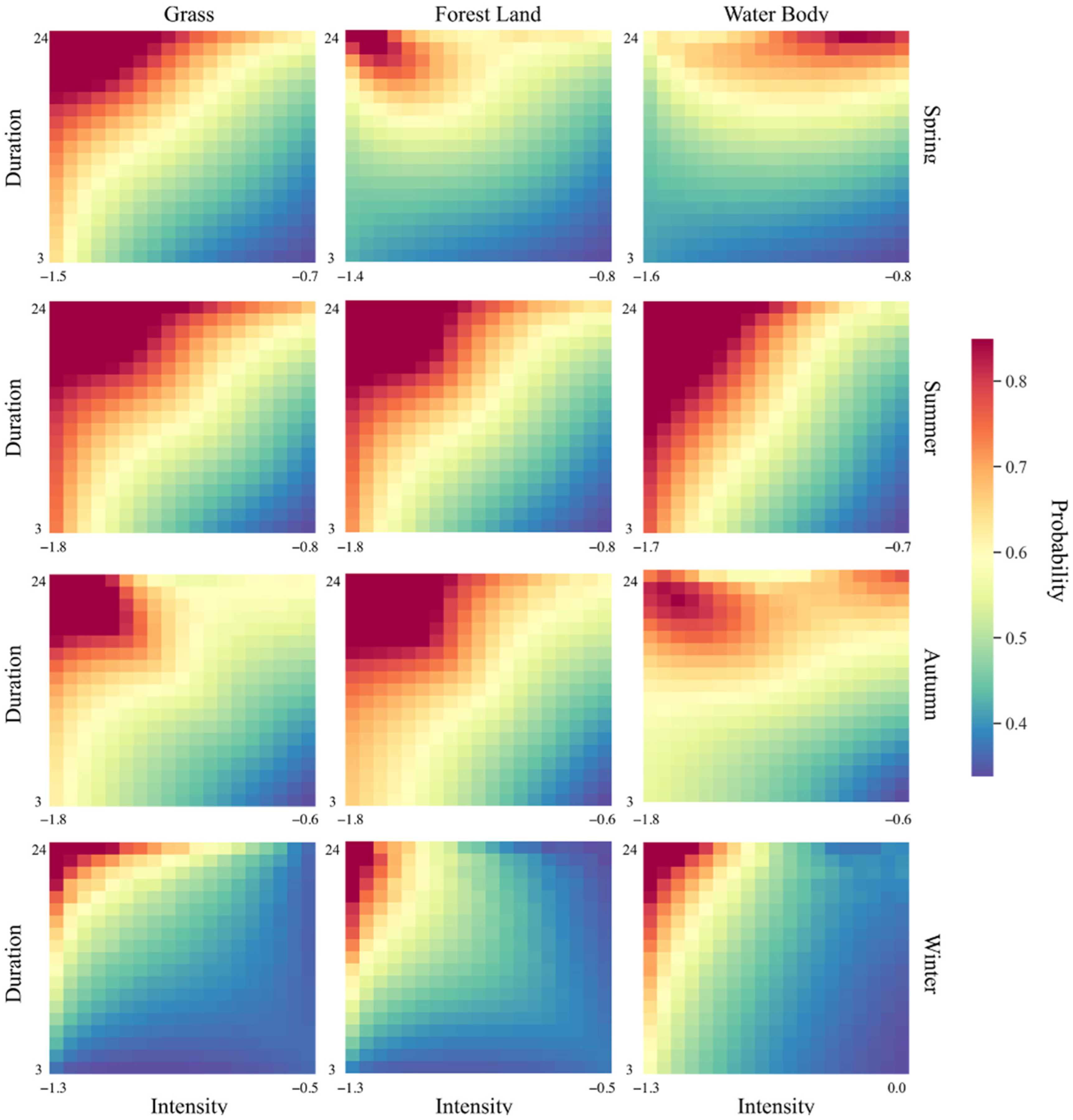
5.2. Drought Vulnerability across Vegetation Types and Seasonal Variations
6. Conclusions
Author Contributions
Funding
Data Availability Statement
Conflicts of Interest
References
- Shin, H. A critical review of robot research and future research opportunities: Adopting a service ecosystem perspective. Int. J. Contemp. Hosp. Manag. 2022, 34, 2337–2358. [Google Scholar] [CrossRef]
- Lin, L.; Wei, X.; Luo, P.; Wang, S.; Kong, D.; Yang, J. Ecological Security Patterns at Different Spatial Scales on the Loess Plateau. Remote Sens. 2023, 15, 1011. [Google Scholar] [CrossRef]
- Costanza, R. Valuing natural capital and ecosystem services toward the goals of efficiency, fairness, and sustainability. Ecosyst. Serv. 2020, 43, 101096. [Google Scholar] [CrossRef]
- Hasan, S.; Zhen, L.; Miah, M.; Ahamed, T.; Samie, A. Impact of land use change on ecosystem services: A review. Environ. Dev. 2020, 34, 100527. [Google Scholar] [CrossRef]
- Pan, F.; Shu, N.; Wan, Q.; Huang, Q. Land Use Function Transition and Associated Ecosystem Service Value Effects Based on Production-Living-Ecological Space: A Case Study in the Three Gorges Reservoir Area. Land 2023, 12, 391. [Google Scholar] [CrossRef]
- Xie, L.; Wang, H.; Liu, S. The ecosystem service values simulation and driving force analysis based on land use/land cover: A case study in inland rivers in arid areas of the Aksu River Basin, China. Ecol. Indic. 2022, 138, 108828. [Google Scholar] [CrossRef]
- Yu, H.; Yang, J.; Sun, D.; Li, T.; Liu, Y. Spatial Responses of Ecosystem Service Value during the Development of Urban Agglomerations. Land 2022, 11, 165. [Google Scholar] [CrossRef]
- Ding, M.; Liu, W.; Xiao, L.; Zhong, F.; Lu, N.; Zhang, J.; Zhang, Z.; Xu, X.; Wang, K. Construction and optimization strategy of ecological security pattern in a rapidly urbanizing region: A case study in central-south China. Ecol. Indic. 2022, 136, 108604. [Google Scholar] [CrossRef]
- Zhu, S.; Huang, J.; Zhao, Y. Coupling coordination analysis of ecosystem services and urban development of resource-based cities: A case study of Tangshan city. Ecol. Indic. 2022, 136, 108706. [Google Scholar] [CrossRef]
- Peng, K.; Jiang, W.; Ling, Z.; Hou, P.; Deng, Y. Evaluating the potential impacts of land use changes on ecosystem service value under multiple scenarios in support of SDG reporting: A case study of the Wuhan urban agglomeration. J. Clean. Prod. 2021, 307, 127321. [Google Scholar] [CrossRef]
- Jiang, Y.; Guan, D.; He, X.; Yin, B.; Zhou, L.; Sun, L.; Huang, D.; Li, Z.; Zhang, Y. Quantification of the coupling relationship between ecological compensation and ecosystem services in the Yangtze River Economic Belt, China. Land Use Policy 2022, 114, 105995. [Google Scholar] [CrossRef]
- Pan, N.; Guan, Q.; Wang, Q.; Sun, Y.; Li, H.; Ma, Y. Spatial Differentiation and Driving Mechanisms in Ecosystem Service Value of Arid Region:A case study in the middle and lower reaches of Shule River Basin, NW China. J. Clean. Prod. 2021, 319, 128718. [Google Scholar] [CrossRef]
- Wu, J.; Wang, G.; Chen, W.; Pan, S.; Zeng, J. Terrain gradient variations in the ecosystem services value of the Qinghai-Tibet Plateau, China. Glob. Ecol. Conserv. 2022, 34, e02008. [Google Scholar] [CrossRef]
- Liang, J.; Xie, Y.; Sha, Z.; Zhou, A. Modeling urban growth sustainability in the cloud by augmenting Google Earth Engine (GEE). Comput. Environ. Urban Syst. 2020, 84, 101542. [Google Scholar] [CrossRef]
- Ma, S.; Huang, J.; Chai, Y. Proposing a GEE-Based Spatiotemporally Adjusted Value Transfer Method to Assess Land-Use Changes and Their Impacts on Ecosystem Service Values in the Shenyang Metropolitan Area. Sustainability 2021, 13, 12694. [Google Scholar] [CrossRef]
- Fathi-Taperasht, A.; Shafizadeh-Moghadam, H.; Sadian, A.; Xu, T.; Nikoo, M.R. Drought-induced vulnerability and resilience of different land use types using time series of MODIS-based indices. Int. J. Disaster Risk Reduct. 2023, 91, 103703. [Google Scholar] [CrossRef]
- Li, Y.; Zhang, W.; Schwalm, C.R.; Gentine, P.; Smith, W.K.; Ciais, P.; Kimball, J.S.; Gazol, A.; Kannenberg, S.A.; Chen, A.; et al. Widespread spring phenology effects on drought recovery of Northern Hemisphere ecosystems. Nat. Clim. Chang. 2023, 13, 182–188. [Google Scholar] [CrossRef]
- Liu, Y.; You, C.; Zhang, Y.; Chen, S.; Zhang, Z.; Li, J.; Wu, Y. Resistance and resilience of grasslands to drought detected by SIF in inner Mongolia, China. Agric. For. Meteorol. 2021, 308–309, 108567. [Google Scholar] [CrossRef]
- Machado-Silva, F.; Peres, L.F.; Gouveia, C.M.; Enrich-Prast, A.; Peixoto, R.B.; Pereira, J.M.C.; Marotta, H.; Fernandes, P.J.F.; Libonati, R. Drought Resilience Debt Drives NPP Decline in the Amazon Forest. Global Biogeochem. Cycles 2021, 35, e2021GB007004. [Google Scholar] [CrossRef]
- Xu, C.; Ke, Y.; Zhou, W.; Luo, W.; Ma, W.; Song, L.; Smith, M.D.; Hoover, D.L.; Wilcox, K.R.; Fu, W.; et al. Resistance and resilience of a semi-arid grassland to multi-year extreme drought. Ecol. Indic. 2021, 131, 108139. [Google Scholar] [CrossRef]
- Yao, Y.; Fu, B.; Liu, Y.; Li, Y.; Wang, S.; Zhan, T.; Wang, Y.; Gao, D. Evaluation of ecosystem resilience to drought based on drought intensity and recovery time. Agric. For. Meteorol. 2022, 314, 108809. [Google Scholar] [CrossRef]
- Liu, X.; Zhu, X.; Pan, Y.; Bai, J.; Li, S. Performance of different drought indices for agriculture drought in the North China Plain. J. Arid Land 2018, 10, 507–516. [Google Scholar] [CrossRef]
- Cai, X.; Zhang, W.; Fang, X.; Zhang, Q.; Zhang, C.; Chen, D.; Cheng, C.; Fan, W.; Yu, Y. Identification of Regional Drought Processes in North China Using MCI Analysis. Land 2021, 10, 1390. [Google Scholar] [CrossRef]
- Jarvis, A.; Reuter, H.I.; Nelson, A.; Guevara, E. Hole-Filled SRTM for the Globe Version 4. CGIAR-CSI SRTM 90 m. 2008. Available online: https://csidotinfo.wordpress.com/data/srtm-90m-digital-elevation-database-v4-1/ (accessed on 13 June 2024).
- Muñoz Sabater, J. ERA5-Land Monthly Averaged Data from 1981 to Present. Copernicus Climate Change Service (C3S) Climate Data Store (CDS). 2019. Available online: https://cds.climate.copernicus.eu/datasets/reanalysis-era5-land-monthly-means?tab=overview (accessed on 18 November 2022).
- Cao, Y.; Kong, L.; Zhang, L.; Ouyang, Z. The balance between economic development and ecosystem service value in the process of land urbanization: A case study of China’s land urbanization from 2000 to 2015. Land Use Policy 2021, 108, 105536. [Google Scholar] [CrossRef]
- Xie, G.; Zhang, C.; Zhen, L.; Zhang, L. Dynamic changes in the value of China’s ecosystem services. Ecosyst. Serv. 2017, 26, 146–154. [Google Scholar] [CrossRef]
- Yin, C.; He, Q.; Xie, P.; Liu, Y.; Zhang, Y.; Chen, W.; Bi, Q. Spatiotemporal variation of the ecosystem service value in China based on surface area. Ecol. Indic. 2023, 148, 110067. [Google Scholar] [CrossRef]
- Gao, F.; Cui, J.; Zhang, S.; Xin, X.; Zhang, S.; Zhou, J.; Zhang, Y. Spatio-Temporal distribution and driving factors of ecosystem service value in a fragile hilly area of North China. Land 2022, 11, 2242. [Google Scholar] [CrossRef]
- Xu, D.; Ding, X. Assessing the impact of desertification dynamics on regional ecosystem service value in North China from 1981 to 2010. Ecosyst. Serv. 2018, 30, 172–180. [Google Scholar] [CrossRef]
- Chi, D.; Wang, H.; Li, X.; Liu, H.; Li, X. Estimation of the ecological water requirement for natural vegetation in the Ergune River basin in Northeastern China from 2001 to 2014. Ecol. Indic. 2018, 92, 141–150. [Google Scholar] [CrossRef]
- O’Connor, R.C.; Germino, M.J.; Barnard, D.M.; Andrews, C.M.; Bradford, J.B.; Pilliod, D.S.; Arkle, R.S.; Shriver, R.K. Small-scale water deficits after wildfires create long-lasting ecological impacts. Environ. Res. Lett. 2020, 15, 044001. [Google Scholar] [CrossRef]
- Vicente-Serrano, S.M.; Miralles, D.G.; Domínguez-Castro, F.; Azorin-Molina, C.; Kenawy, A.E.; McVicar, T.R.; Tomás-Burguera, M.; Beguería, S.; Maneta, M.; Peña-Gallardo, M. Global Assessment of the Standardized Evapotranspiration Deficit Index (SEDI) for Drought Analysis and Monitoring. J. Clim. 2018, 31, 5371–5393. [Google Scholar] [CrossRef]
- Deb, P.; Kiem, A.S.; Willgoose, G. A linked surface water-groundwater modelling approach to more realistically simulate rainfall-runoff non-stationarity in semi-arid regions. J. Hydrol. 2019, 575, 273–291. [Google Scholar] [CrossRef]
- Jiang, T.; Su, X.; Singh, V.P.; Zhang, G. A novel index for ecological drought monitoring based on ecological water deficit. Ecol. Indic. 2021, 129, 107804. [Google Scholar] [CrossRef]
- Zamani Losgedaragh, S.; Rahimzadegan, M. Evaluation of SEBS, SEBAL, and METRIC models in estimation of the evaporation from the freshwater lakes (Case study: Amirkabir dam, Iran). J. Hydrol. 2018, 561, 523–531. [Google Scholar] [CrossRef]
- McKee, T.B.; Doesken, N.J.; Kleist, J. The relationship of drought frequency and duration to time scales. In Proceedings of the 8th Conference on Applied Climatology, Anaheim, CA, USA, 17–22 January 1993; pp. 179–183. [Google Scholar]
- Mesbahzadeh, T.; Mirakbari, M.; Mohseni Saravi, M.; Soleimani Sardoo, F.; Miglietta, M.M. Meteorological drought analysis using copula theory and drought indicators under climate change scenarios (RCP). Meteorol. Appl. 2020, 27, e1856. [Google Scholar] [CrossRef]
- Zou, X.; Zhai, P.; Zhang, Q. Variations in droughts over China: 1951–2003. Geophys. Res. Lett. 2005, 32, L04707. [Google Scholar] [CrossRef]
- Shao, D.; Chen, S.; Tan, X.; Gu, W. Drought characteristics over China during 1980–2015. Int. J. Climatol. 2018, 38, 3532–3545. [Google Scholar] [CrossRef]
- Huang, J.; Xue, Y.; Sun, S.; Zhang, J. Spatial and temporal variability of drought during 1960–2012 in inner mongolia, north china. Quat. Int. 2015, 355, 134–144. [Google Scholar] [CrossRef]
- Ma, Z.; Sun, P.; Zhang, Q.; Hu, Y.; Jiang, W. Characterization and evaluation of MODIS-derived crop water stress index (CWSI) for monitoring drought from 2001 to 2017 over inner mongolia. Sustainability 2021, 13, 916. [Google Scholar] [CrossRef]
- Kang, Y.; Guo, E.; Wang, Y.; Bao, Y.; Mandula, N. Monitoring vegetation change and its potential drivers in inner mongolia from 2000 to 2019. Remote Sens. 2021, 13, 3357. [Google Scholar] [CrossRef]
- Gong, Z.; Kawamura, K.; Ishikawa, N.; Goto, M.; Wulan, T.; Alateng, D.; Yin, T.; Ito, Y. MODIS normalized difference vegetation index (NDVI) and vegetation phenology dynamics in the inner mongolia grassland. Solid Earth 2015, 6, 1185–1194. [Google Scholar] [CrossRef]
- An, Q.; He, H.; Nie, Q.; Cui, Y.; Gao, J.; Wei, C.; Xie, X.; You, J. Spatial and temporal variations of drought in inner mongolia, china. Water 2020, 12, 1715. [Google Scholar] [CrossRef]
- Jiang, T.; Su, X.; Zhang, G.; Zhang, T.; Wu, H. Estimating propagation probability from meteorological to ecological droughts using a hybrid machine learning copula method. Hydrol. Earth Syst. Sci. 2023, 27, 559–576. [Google Scholar] [CrossRef]
- Wu, Z.; Wu, J.; He, B.; Liu, J.; Wang, Q.; Zhang, H.; Liu, Y. Drought offset ecological restoration program-induced increase in vegetation activity in the beijing-tianjin sand source region, china. Environ. Sci. Technol. 2014, 48, 12108–12117. [Google Scholar] [CrossRef] [PubMed]
- Huang, W.; Wang, W.; Cao, M.; Fu, G.; Xia, J.; Wang, Z.; Li, J. Local climate and biodiversity affect the stability of China’s grasslands in response to drought. Sci. Total Environ. 2021, 768, 145482. [Google Scholar] [CrossRef]
- Kowalski, K. Large-scale remote sensing analysis reveals an increasing coupling of grassland vitality to atmospheric water demand. Glob. Chang. Biol. 2024, 30, 5. [Google Scholar] [CrossRef]
- Lu, M. Heterogeneity in vegetation recovery rates post-flash droughts across different ecosystems. Environ. Res. Lett. 2024, 19, 074028. [Google Scholar] [CrossRef]
- Shinohara, Y.; Otsuki, K. Comparisons of soil-water content between a moso bamboo (Phyllostachys pubescens) forest and an evergreen broadleaved forest in western Japan. Plant Species Biol. 2015, 30, 96–103. [Google Scholar] [CrossRef]
- Deng, J.; Yin, Y.; Zhu, W.; Zhou, Y. Variations in soil bacterial community diversity and structures among different revegetation types in the Baishilazi Nature Reserve. Front. Microbiol. 2018, 9, 02874. [Google Scholar] [CrossRef]
- Vicente-Serrano, S.M.; Quiring, S.M.; Peña-Gallardo, M.; Yuan, S.; Domínguez-Castro, F. A review of environmental droughts: Increased risk under global warming? Earth-Sci. Rev. 2020, 201, 102953. [Google Scholar] [CrossRef]
- Loon, A.F.V.; Tijdeman, E.; Wanders, N.; Lanen, H.V.; Teuling, A.J.; Uijlenhoet, R. How climate seasonality modifies drought duration and deficit. J. Geophys. Res. Atmos. 2014, 119, 4640–4656. [Google Scholar] [CrossRef]
- Saeidnia, F.; Majidi, M.M.; Mirlohi, A.; Soltan, S. Physiological and tolerance indices useful for drought tolerance selection in smooth bromegrass. Crop Sci. 2017, 57, 282–289. [Google Scholar] [CrossRef]
- Vogrinc, P.; Durso, A.; Winne, C.; Willson, J. Landscape-scale effects of supra-seasonal drought on semi-aquatic snake assemblages. Wetlands 2018, 38, 667–676. [Google Scholar] [CrossRef]


| Service Function | Cropland | Forest Land | Grassland | Water Body | Building | Bare Land | |
|---|---|---|---|---|---|---|---|
| Regulating Services | Air purification | 0.5 | 3.5 | 0.8 | 0 | 0 | 0 |
| Climate regulation | 0.89 | 2.7 | 0.9 | 0.46 | 0 | 0 | |
| Water regulation | 1.64 | 1.31 | 1.31 | 18.2 | 0 | 0.01 | |
| Provisioning Services | Food production | 1 | 0.1 | 0.3 | 0.1 | 0 | 0.01 |
| Water supply | 0.6 | 3.2 | 0.8 | 20.4 | 0 | 0.03 | |
| Raw materials | 0.1 | 2.6 | 0.05 | 0.01 | 0 | 0 | |
| Supporting Services | Soil conservation | 1.46 | 3.9 | 1.95 | 0.01 | 0 | 0.03 |
| Biodiversity | 0.71 | 3.26 | 1.09 | 2.49 | 0 | 0.34 | |
| Cultural Services | Aesthetic landscape | 0.01 | 1.28 | 0.04 | 4.34 | 1.12 | 0.01 |
Disclaimer/Publisher’s Note: The statements, opinions and data contained in all publications are solely those of the individual author(s) and contributor(s) and not of MDPI and/or the editor(s). MDPI and/or the editor(s) disclaim responsibility for any injury to people or property resulting from any ideas, methods, instructions or products referred to in the content. |
© 2024 by the authors. Licensee MDPI, Basel, Switzerland. This article is an open access article distributed under the terms and conditions of the Creative Commons Attribution (CC BY) license (https://creativecommons.org/licenses/by/4.0/).
Share and Cite
Jiang, T.; Qu, Y.; Zhang, X.; Jing, L.; Feng, K.; Zhang, G.; Han, Y. Evaluating Ecological Drought Vulnerability from Ecosystem Service Value Perspectives in North China. Remote Sens. 2024, 16, 3733. https://doi.org/10.3390/rs16193733
Jiang T, Qu Y, Zhang X, Jing L, Feng K, Zhang G, Han Y. Evaluating Ecological Drought Vulnerability from Ecosystem Service Value Perspectives in North China. Remote Sensing. 2024; 16(19):3733. https://doi.org/10.3390/rs16193733
Chicago/Turabian StyleJiang, Tianliang, Yanping Qu, Xuejun Zhang, Lanshu Jing, Kai Feng, Gengxi Zhang, and Yu Han. 2024. "Evaluating Ecological Drought Vulnerability from Ecosystem Service Value Perspectives in North China" Remote Sensing 16, no. 19: 3733. https://doi.org/10.3390/rs16193733