Article

Evaluating Ecological Drought Vulnerability from Ecosystem Service Value Perspectives in North China

1
Institute of Water Resources and Hydropower Research, Beijing 100038, China
2
Research Center on Flood and Drought Disaster Reduction of the Ministry of Water Resources, Beijing 100038, China
3
College of Water Conservancy, North China University of Water Resources and Electric Power, Zhengzhou 450045, China
4
College of Hydraulic Science and Engineering, Yangzhou University, Yangzhou 225012, China
*
Author to whom correspondence should be addressed.
Remote Sens. 2024, 16(19), 3733; https://doi.org/10.3390/rs16193733
Submission received: 21 August 2024 / Revised: 1 October 2024 / Accepted: 2 October 2024 / Published: 8 October 2024

Abstract

:
Existing studies on the vulnerability assessment of ecological drought often focus on analyzing vegetation phenotypic characteristics, overlooking the impact of drought on ecosystem services. This study proposes an ecosystem vulnerability assessment method under ecological drought stress from the perspective of ecosystem service value (ESV), considering the characteristics and interactions of hazard-causing factors and hazard-bearing bodies. The spatiotemporal evolution of ecological drought, the spatial characteristics of ecosystem vulnerability, and the vulnerability characteristics of different ecosystem types in the North China region from 1991 to 2021 were evaluated. The results showed that: (1) ecological drought exhibited a trend of intensification followed by alleviation, with the most severe droughts occurring between 2002 and 2011, affecting up to 64.3% of the region; (2) ESV was mainly influenced by vegetation cover and precipitation gradients, displaying a spatial pattern of high values in the southeast and low values in the northwest, with total ESV averaging CNY 18.23 trillion; (3) grasslands exhibited higher sensitivity to drought compared to forests, and the sensitivity was higher in summer and autumn than in winter and spring. This method assessed the vulnerability of ecological drought from the perspective of ecosystem services, providing a new approach for a more comprehensive understanding of the impact of drought on ecosystem service functions.

1. Introduction

Ecosystems provide many valuable services, such as provisioning services like food and water, regulating services like climate and flood regulation, cultural services like recreation, and supporting services like nutrient cycling [1]. However, China’s rapid economic growth in recent decades has led to considerable ecosystem degradation through processes like urbanization, agricultural intensification, and pollution [2]. Quantifying ecosystem service values (ESV) is crucial for understanding the true economic costs of ecosystem changes, guiding sustainable development policies, and demonstrating the value of natural capital in economic terms [3]. Studying ESV enables policymakers to make more informed decisions regarding tradeoffs between economic development and environmental protection. For example, one study found that from 2000 to 2010, China’s ESV decreased by USD 0.9–1.3 trillion annually due to land use changes associated with urbanization and agricultural expansion [4]. This massive loss of ESV underscores the need for China to account for natural capital in policy-making. Thus, ecosystem services research is growing rapidly in China to quantify ESV, inform environmental policy, and promote sustainable development.
Previous ESV assessments in China have mostly focused on national and provincial aggregate scales using data like land use/land cover maps [5,6,7]. However, high-resolution land use type data for evaluating ecosystem service values are still lacking for many specific regions. One area requiring further study is the North China region, spanning Beijing, Tianjin, Shanxi, Shandong, Hebei, and Inner Mongolia. As a highly populated and agriculturally important zone in northern China, the North China region boasts rich natural resources but has faced severe environmental problems like water scarcity, soil erosion, and sandstorms amid rapid industrialization and urbanization in past decades [8]. In response, China has implemented ecological restoration programs like the Grain for Green Program in the North China Plain to convert steep croplands to forests and grasslands [9]. Following the implementation of these ecological projects, it is crucial to investigate the changes in ecosystem service values to assess the effectiveness of these initiatives. Quantifying the dynamics of ecosystem service values in the North China Plain after restoration efforts is of great practical significance for addressing ecological issues and guiding future ecological management in the region [10].
Google Earth Engine (GEE) provides a powerful platform for efficiently mapping land cover over large areas, an essential initial step for estimating ESV [1,4,11]. While GEE has been utilized in some recent ESV assessments for China, these studies have been limited in their temporal resolution [5,6,9,10,12,13]. For instance, previous GEE-based research calculated ESV at annual intervals. GEE enables the efficient processing of vast amounts of satellite imagery, allowing for land cover mapping at higher temporal resolutions than previously feasible [14,15]. This frequent land cover mapping can then be utilized to estimate changes in ESV at these finer time steps, revealing new insights into how ESV responds to seasonal factors and random shocks. Additionally, machine learning methods could be implemented on GEE to automate land cover classification and ESV modeling, enabling near real-time monitoring [14]. Therefore, harnessing GEE’s spatiotemporal power can significantly advance ESV assessments in the North China region by providing finer-grained analysis over broader extents and longer time periods.
In most existing studies, ecosystem vulnerability to drought has been evaluated primarily from the perspective of the ecosystem itself, which fails to reflect the impact of drought on ecosystem services. Most existing ecological drought studies focus on analyzing meteorological factors like precipitation deficits to characterize drought intensity, while lacking quantitative assessment of consequent ecosystem service losses [16,17,18,19,20,21,22]. However, quantifying the relationship between changes in ecosystem service values and drought dynamics can better reflect the impacts of drought on ecosystem service functions. Therefore, an integrated approach coupling ecosystem service evaluation with ecological drought monitoring is needed to evaluate how drought events affect the supply and value of services from ecosystems. Furthermore, evaluating the vulnerability of ecosystem service provision to drought can support cost–benefit analysis of drought adaptation strategies and inform decision-making for ecological management. Addressing this research gap by linking ecological drought with ecosystem service consequences is crucial for developing effective drought resilience measures and mitigating the adverse impacts of droughts on ecosystems and their services.
To address these issues, this study leverages GEE to assess the monthly dynamics of ecosystem service values (ESV) and ecological drought vulnerability across the North China Plain from 1991 to 2021. ESV changes were quantified at a monthly scale and with fine spatial resolution, revealing localized ESV patterns related to terrain, ecosystems, and human activities. Ecological drought in NC was analyzed using the standardized water deficit index, linking spatiotemporal drought patterns with ESV fluctuations to quantitatively assess ecosystem vulnerability. Overall, this integrated approach offers new perspectives on the ecological and economic impacts of environmental changes in North China, supporting ecosystem management and ecological restoration program evaluation.

2. Materials

2.1. Study Region

The study region encompasses North China (Figure 1). Specifically, this study focuses on the six provincial-level administrative units that make up North China: Beijing, Tianjin, Shanxi, Shandong, Hebei, and Inner Mongolia. This region covers an area of approximately 1.3 million km2 and had a population of 359 million in 2010 [22]. The North China Plain features a warm temperate monsoon climate, with hot rainy summers and cold dry winters. Mean annual precipitation ranges from 400 to 800 mm, decreasing from southeast to northwest across the region. Major ecosystem types include cultivated land, forests, grasslands, and inland water bodies. Forests are concentrated in mountainous areas while agriculture dominates the fertile plains. The main land cover changes in recent decades have been agricultural expansion, reforestation, and urban growth [23].

2.2. Dataset

This study utilized three main types of datasets—geospatial data, topographic data, and vegetation data. The geospatial data were obtained from Google Earth Engine (GEE), including Landsat 5 TM, Landsat 7 ETM+, and Landsat 8 OLI imagery. Specifically, the Landsat 5 TM images spanned from 1984 to 2011 with a spatial resolution of 30 m. Landsat 7 ETM+ images were from 1999 to the present with a spatial resolution of 30 m. And Landsat 8 OLI images covered 2013 to the present with a spatial resolution of 30 m. The topographic data were the SRTM digital elevation model (DEM) provided by NASA/USGS/JPL Caltech [24], which had a spatial resolution of 90 m. Vegetation data consisted of the Normalized Difference Vegetation Index (NDVI), which was obtained from composite Landsat NDVI datasets downloaded from http://www.gis5g.com/data/zbsj/NDVI (accessed on 14 June 2024), with a spatial resolution of 30 m, ensuring consistency across the study period. Meteorological datasets, including monthly precipitation and monthly temperatures spanning from 1979 to present with a spatial resolution of 0.25° × 0.25°, were derived from the ERA-Interim reanalysis dataset produced by the European Center for Medium-Range Weather Forecasts (ECMWF) [25]. Agricultural data, including food production and yield prices, were sourced from the National Bureau of Statistics of China, available through their publicly accessible database: https://data.stats.gov.cn/ (accessed on 3 June 2024).

3. Method

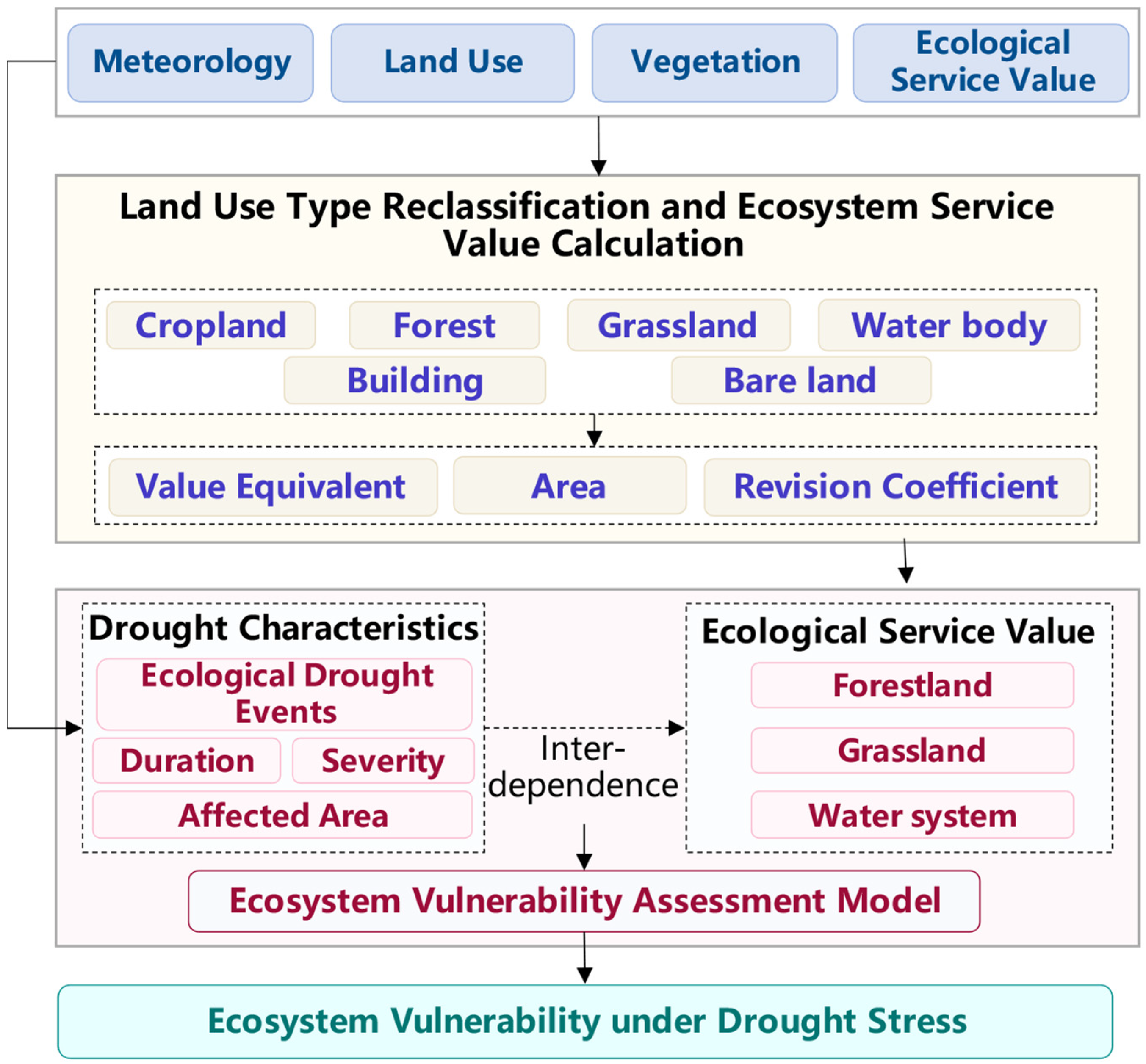
This study employs a three-step methodology: data processing, land use type reclassification, ecosystem service value (ESV) calculation, and the construction of an ecosystem vulnerability assessment model (Figure 2). The data processing step involves the integration of meteorology, land use, vegetation, and ecosystem service value equivalent data, providing the necessary foundation for land use type reclassification, ESV calculation, and drought characteristics identification. The assessment of ESV is a crucial component of the research, serving as input for the vulnerability assessment model. By establishing an evaluation model, the spatial distribution of vulnerability under drought stress is determined for the study area.

3.1. Optimizing Land Use Classification Based on Google Earth Engine

In this study, land use classification was conducted in three steps:
(1) Preprocessing of the original remote sensing images to obtain high-quality images that meet the training requirements.
The Google Earth Engine “Reducer” function was used to perform atmospheric correction on the original integrated geospatial dataset using the LaSRC algorithm, and the CFMask algorithm was used to mask clouds, shadows, water, and snow in the images to obtain high-quality annual image sequences. Normalized Difference Vegetation Index (NDVI) was overlaid on the data images for each year to increase model complexity, and a DEM was added to distinguish plains and mountains. Finally, the data were standardized to reduce noise and classification errors in the remote sensing images.
(2) Preliminary classification of the original datasets (including selection of an appropriate classification system, classifiers, training samples, and test samples).
In this study, a first-level land use classification system was used, including cropland, forest, grassland, water bodies, buildings, and bare land. The Cart, Random Forest, Gradient Boosting Regression, and Support Vector models in GEE were used as classifiers to perform supervised classification learning on the images for each year. The training samples for the models were extracted and classified for each year based on the high-resolution images, generating a total of 2000 × 31 labeled points. Datasets for the input contained seven spectral bands (Band 1-Band 7) from Landsat 5, Landsat 7, and Landsat 8, as well as slope information derived from the processed DEM. A total of 70% of the data were used as training samples and 30% as test samples. The Kappa metrics were used to evaluate the classification results for each year and select the best-performing classifier. Ultimately, the optimal classifier was applied to conduct the preliminary classification of the original dataset, ensuring the highest accuracy and minimizing classification errors in the land use mapping process.
(3) Post-processing of the preliminary classification results to reduce errors in spatial-temporal consistency.
The preliminary land type classification based on machine learning often leads to inconsistencies in the evaluation results over space and time. To address this issue, Python APIs based on the GEE platform were developed in this study, constructing “Spatial_Analysis” functions to resolve spatial inconsistency and “Temporal_Analysis” functions to resolve temporal inconsistency.
I “Spatial_Analysis” function
For spatial inconsistencies, a nine-pixel pooling grid was used to traverse the preliminary classification results. When the center value of a grid was inconsistent in space, it was corrected using the land type with the highest proportion among the surrounding eight pixels.
II “Temporal_Analysis” function
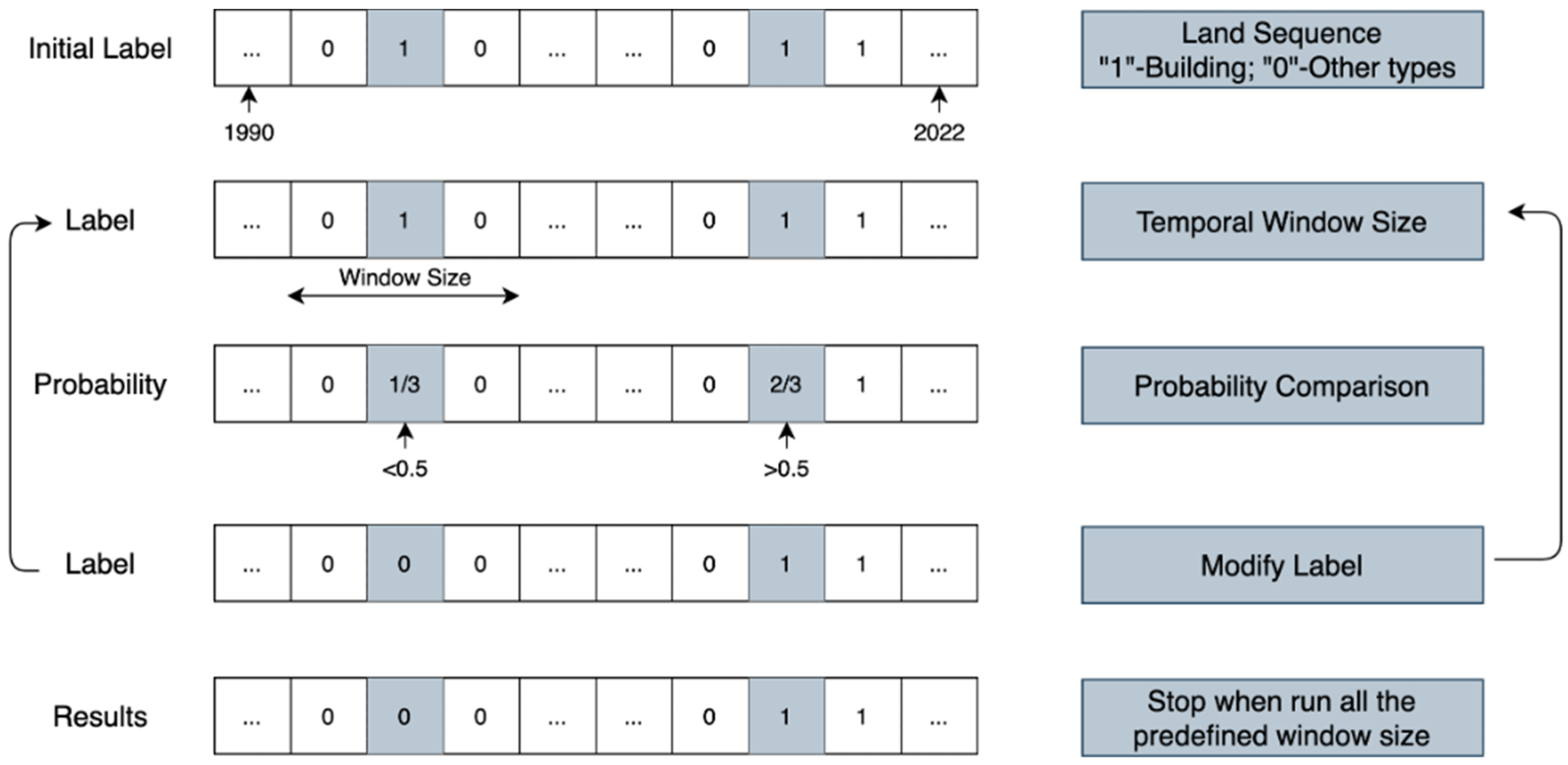
For temporal inconsistencies, this study mainly resolved instability in built-up land over time, such as cases where a pixel was classified as built-up land in 2000 and 2002 but forest land in 2001. Therefore, sliding windows of a certain step size were used to calculate the temporal consistency probability of each pixel, thereby enabling correction of deviations in the classification results [14] (Figure 3).
P r o b i = j = i T w j = i + T w con ( L j = L i ) 1 + 2 × ( T w )
where T w is the predefined time window, set to 3 in this study; L i is the land use type label for the target year; L j is the land use type label for the adjacent year; con is a logic judgment function, returning 1 if L i = L j , otherwise returning 0; a larger Prob value indicates a higher probability that L i is true. In this study, 0.5 was taken as the critical threshold, that is, L i is changed to L j when P r o b i > 0.5.

3.2. Constructing Ecosystem Service Value Dynamic Assessment Methods Based on Google Earth Engine

Different ecosystem types have different ecological processes, thereby providing different levels of ecosystem services [26]. To further improve the objectivity and rationality of ecosystem service value assessment results, Python APIs running on the GEE platform were developed in this study to incorporate precipitation (P), NDVI (C), and coverage (S) as modulation factors. This allows for the ecosystem service value results to reflect the quantity and functional information of ecosystems.
E S V n 1 = i = 1 m j = 1 n k = 1 o A k B i j k C k
C k = N D V I k ¯ N D V I ¯
E S V n 2 = i = 1 m j = 1 n k = 1 o A k B i j k P k
P k = W k W ¯
E S V n 3 = i = 1 m j = 1 n k = 1 o A k B i j k S k
S k = E k E ¯
E S V = E S V n 1 + E S V n 2 + E S V n 3
where i, j, and k represent land use type (including cropland, forest, grassland, water body, buildings, and bare land), ecosystem service type (including three provisioning services, three regulating services, two supporting services, and one cultural service), and the number of each pixel, respectively. ESVn1 represents the ecosystem services of food production, raw material production, gas regulation, climate regulation, biodiversity, and aesthetic landscape. ESVn2 represents water supply and water flow regulation services. ESVn3 represents soil and water conservation. N D V I ¯ , W ¯ , and F ¯ are the mean NDVI, precipitation, and vegetation coverage of the study area, respectively. N D V I k ¯ , W k ¯ , and F k ¯ are the NDVI, precipitation, and vegetation coverage of the k-th study unit. Ak is the area of the k-th grid cell, and Bijk is the ecosystem service value equivalent coefficient of the j-th service of the i-th land use type in the k-th grid cell. o is the number of pixels.
Accurately assessing Bijk is key and a prerequisite for calculating ESV. To eliminate the impact of price inflation on Bijk, the consumer price index (CPI) was introduced for calibration, and the “Equivalent Value Per Unit Area of Chinese Terrestrial Ecosystem Services” revised twice by [27] (Table 1) was referenced to calculate Bijk:
B i j k = e i j k B 0 , k = 1 , , o
B 0 = B 0 × a n a 0
B 0 = 1 7 × P × 1 n t = 1 n Q i , t = 1 , 2 , 3
a n a 0 = a 1 a 0 × a 2 a 1 × a 3 a 2 × × a n a n 1
where P is the average food price, Q is the average food yield in the study area, n is the number of years, and t represents crop types including wheat, corn, and rice. an/a0 is the current period year-on-year CPI, a1/a0 is last period month-on-month CPI. eijk is the ecosystem service value equivalent coefficient of the j-th service of the i-th ecosystem in the k-th unit, obtained from Table 1, which was determined based on the studies by [28,29,30].

3.3. Constructing Ecological Drought Index

3.3.1. Ecological Water Deficit

Based on the concept and formation mechanism of ecological drought, the ecological drought index should have the ability to identify the degree of water deficit from an ecological perspective. Most existing studies use the difference between effective precipitation and ecological water requirement to calculate ecological water deficit [31]. However, this method treats precipitation as a water supply, ignoring other water resources for vegetation growth such as groundwater [32]. Therefore, Vicente-Serrano et al. suggested that actual evapotranspiration of vegetation instead of effective precipitation should represent ecosystem water supply, and the evapotranspiration deficit obtained by subtracting ecological water requirement can better characterize ecological water deficit (EWD) [33].
E W D = E W C E W R
where E W C represents ecological water consumption; EWR represents ecological water requirement.
E W R reflects the maximum water requirement at ideal conditions to maintain ecosystem health and function [34]. This study adopted the single crop coefficient method recommended by the Federal Agricultural Organization (FAO) to calculate it, which has been widely used to estimate forest and grassland water requirements [31].
E W R = k c × E T 0
where kc is the vegetation coefficient for different periods, including the initial stage, development stage, mid-season stage, and late season stage [35]; when the underlying surface consists of water or bare land, the kc equals 1 and 0.3, respectively. ET0 is the reference evapotranspiration of crops, calculated by the Penman–Monteith formula recommended by FAO-56.
E T 0 = 0.408 Δ R n G + γ 900 T + 273 u 2 e s e a Δ + γ 1 + 0.34 u 2
where Δ is the slope of the saturation vapor pressure–temperature curve; Rn is the net radiation flux density at the crop surface; G is the soil heat flux density; γ is the psychrometric constant; T is the mean air temperature; u2 is the average wind speed at 2 m height; es is the saturation vapor pressure; ea is the actual vapor pressure.
EWC refers to the amount of water resources that must be consumed to maintain normal ecological system functions. It was calculated using the surface energy balance (SEBS) model. The SEBS model evaluates EWC mainly by estimating evapotranspiration through latent heat flux under different environments, showing stronger robustness and higher accuracy [36].
R n = ( 1 α ) R s w d + ε R t w d ε σ T 0 4
G 0 = R n Γ e + ( 1 f ) Γ s Γ c
H = ρ C p θ 0 θ a r a c
r a c = ln z d 0 / z 0 2 / k 2 μ
u = u * k ln z d 0 z 0 m Ψ m z d 0 z 0 m + Ψ m z 0 m L
θ 0 θ α = H k u * ρ C p ln z d 0 z 0 h Ψ h z d 0 L + Ψ h z 0 h L
λ E = R n G 0 H
where Rn is net radiation of the land surface; α is surface albedo; Rswd and Rlwd are downward solar radiation and downward longwave radiation; ε is surface emissivity; T 0 4 is radiative land surface temperature measured by the sensor; σ is the Stefan–Boltzmann constant; Γ c is the parameter for fully vegetated areas in the region, usually taken as 0.05; Γ s is the parameter for non-vegetated areas in the region, usually taken as 0.315; ρ represents air density; CP represents air heat capacity; θ0 represents land surface potential temperature; θa represents air potential temperature at the reference height; rac is aerodynamic resistance; z is the reference height (usually 2 m); d0 is the height of the horizontal plane; k is the Karman constant, taken as 0.4; z0 is the surface roughness length, m, usually affected by vegetation height and closure; μ is wind speed at the reference height; u is average wind speed; u* is friction velocity; d0 is the height of the horizontal plane; z is the reference height for obtaining meteorological data, generally 2~10 m; z0m is the dynamic roughness length, z0h is the thermal conductivity relative roughness; Ψm and Ψh are the MOS stability correction functions for momentum and heat transfer on the surface; θ0 represents land surface potential temperature; θa represents air potential temperature at the reference height z; Cp is air heat capacity; H is sensible heat flux; g is gravitational acceleration; L is Obukhov length; θv is near-surface virtual potential temperature. By iteratively substituting the above formulas into the computer, u*, H, and L can be obtained, and then the latent heat flux λE and ETa:
H d = R n G 0
λ E w = R n G 0 H w
Λ r = λ E λ E w = 1 λ E w λ E λ E w = 1 H H w H d H w
Λ = λ E R n G 0 = Λ r λ E w R n G 0
E T a = Λ R n G 0 λ ρ w
where H w and H d represent sensible heat flux under extremely dry and wet conditions; Λ r is the relative evaporation ratio; Λ is the evaporation ratio; λ is the latent heat of vaporization; ρ w is water density.

3.3.2. Standardized Ecological Water Deficit Index

Drought indices constructed based on standardization methods have advantages such as spatial comparability, containing probability information, and ease of calculation and interpretation [37]. Therefore, this study standardized the ecological water deficit to obtain the standardized ecological water deficit index to characterize ecological drought. The specific steps are as follows: (1) Normalize the ecological water deficit sequence x1i to obtain the new sequence x2i, with the maximum and minimum values calculated based on the entire time series for each pixel from January to December over the period from 1991 to 2021. To fit the distribution and avoid extreme values, 0.999 and 0.001 were used instead of 1 and 0. (2) Fit three commonly used distributions, including Gamma distribution, log-logistic distribution, and P-III distribution to x2i to obtain distribution parameters, and select the optimal fitting distribution using the Akaike Information Criterion (AIC). (3) Integrate the probability density function fx2i(t) of the optimal distribution to obtain the corresponding cumulative distribution function Fx2i(t). (4) Inversely transform Fx2i(t) to obtain the standardized ecological water deficit index (SEWDI).
x 2 i = x 1 i min ( x 1 i ) max ( x 1 i ) min ( x 1 i ) × ( 0.999 0.001 ) + 0.001
F x 2 i x = x f x 2 i t d t
S E W D I = Φ 1 F x 2 i

3.4. Vulnerability Assessment of Ecosystems

Based on the ecological drought index at the three-month scale, drought events and their characteristics (duration, severity, and affected area) in the study area were extracted using run theory [38]. The relationship model between duration, severity, and ecosystem service value (ESV) was constructed using C-vine copula to calculate the probability of ESV loss under different drought scenarios. Finally, the spatial distribution of ecosystem vulnerability in the study area was obtained through spatial autocorrelation analysis and Mann–Kendall trend analysis. The specific model-building process is as follows:
Firstly, build a 3D C-vine copula with the ecosystem service value as the central node, drought duration, and severity. Use bivariate copula functions to jointly model each univariate marginal distribution in pairs to obtain the joint distribution of the three variables.
F ( D , S , E ) = C F D ( d ) , F S ( s ) , F E ( e )
f ( d , s , e ) = f d · f s · f e · c d e · c s e · c d s e
where F D d , F S s , and F E e are the marginal cumulative distribution functions of drought duration, severity, and ecosystem service value; cde and cds|e are abbreviations for c( F D d , F E e ) and c(F(D,E), F(S,E)); and other abbreviations are similar.
Secondly, the Bayesian network conditional probability model is used to solve the problem of ESV response probability under different drought scenarios.
F ( E e D > d , S > s ) = F ( E e , D > d , S > s ) F ( D > d , S > s ) = F E ( e ) C F E ( e ) , F D ( d ) 1 F D ( d ) F S ( s ) + C F S ( s ) , F D ( d ) C F E ( e ) , F S ( s ) C F D ( d ) , F E ( e ) , F S ( s ) 1 F D ( d ) F S ( s ) + C F S ( s ) , F D ( d )
Based on Equation (33), the probability that the quantile of ESV less than 20% under different durations and severity of drought was calculated to generate the vulnerability map of different ecosystem types and their spatiotemporal distribution.

4. Results

4.1. Land Use Change in North China

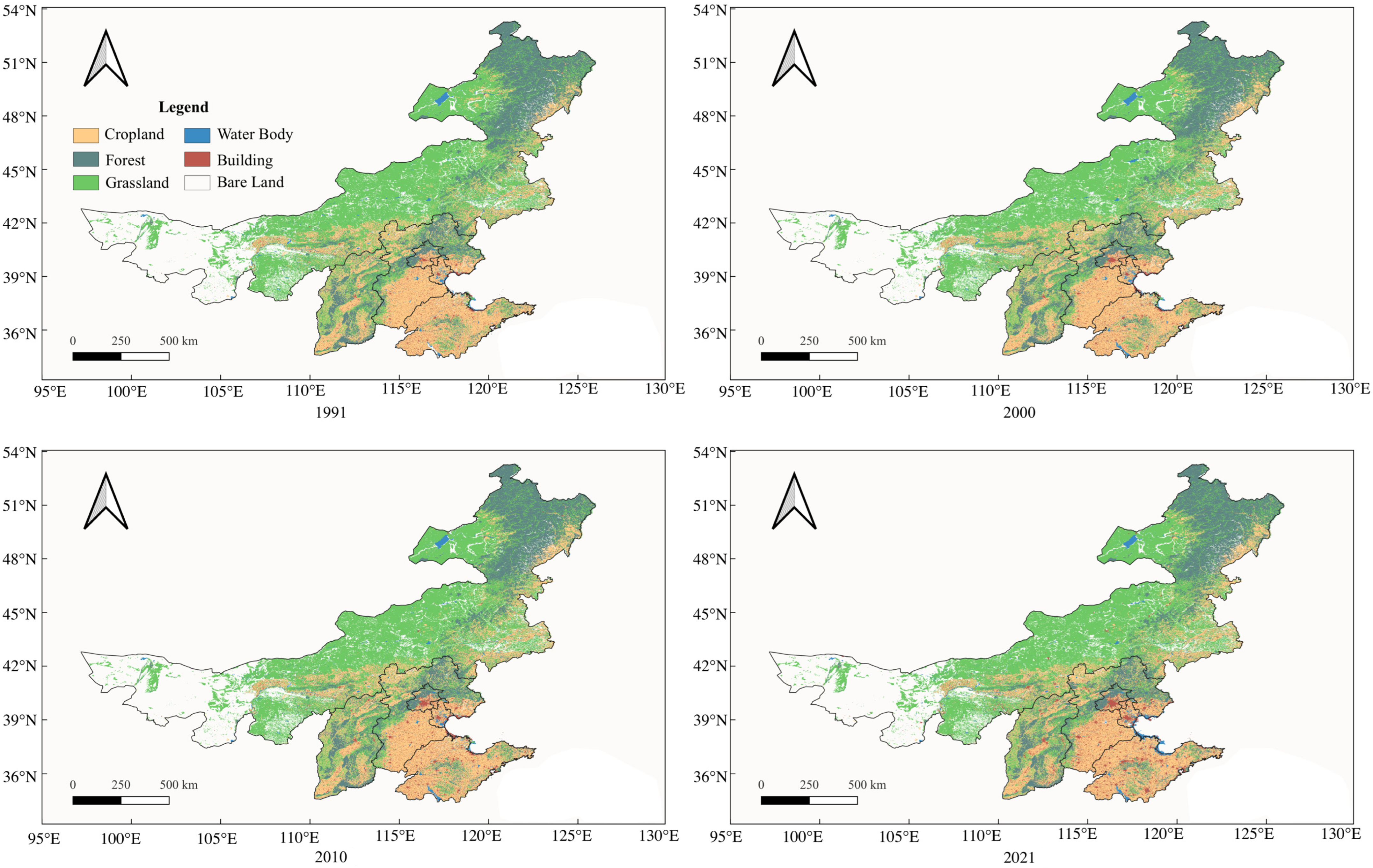
We have generated 1 km resolution land use datasets across North China spanning the period from 1991 to 2021. Figure 4 shows the spatial distribution of land use types in North China for typical years 1991, 2000, 2010, and 2020. It can be seen from the figure that grassland is mainly concentrated in central Inner Mongolia, and forest is mainly in northeast Inner Mongolia and central Shanxi. Cropland mainly concentrates in southern Hebei and Shandong.
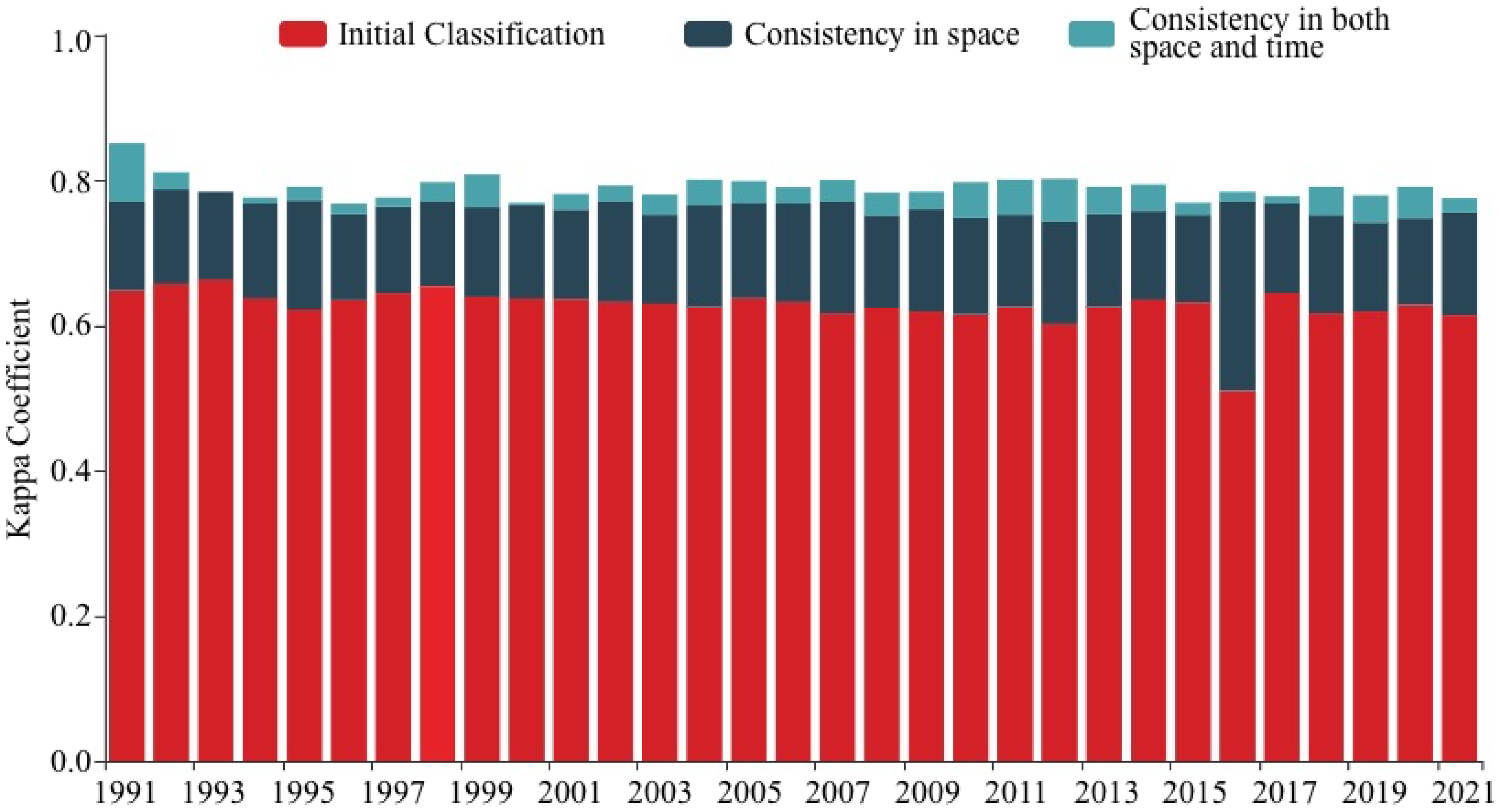
The Kappa index was computed for three different modes. As shown in Figure 5, the accuracy of the land use classification without post-processing is relatively low. The classification that considers only spatial consistency shows moderate improvement, while the classification that takes both spatial and temporal consistency into account achieves the highest accuracy. The improvement in accuracy ranges from 0.12 to 0.26.
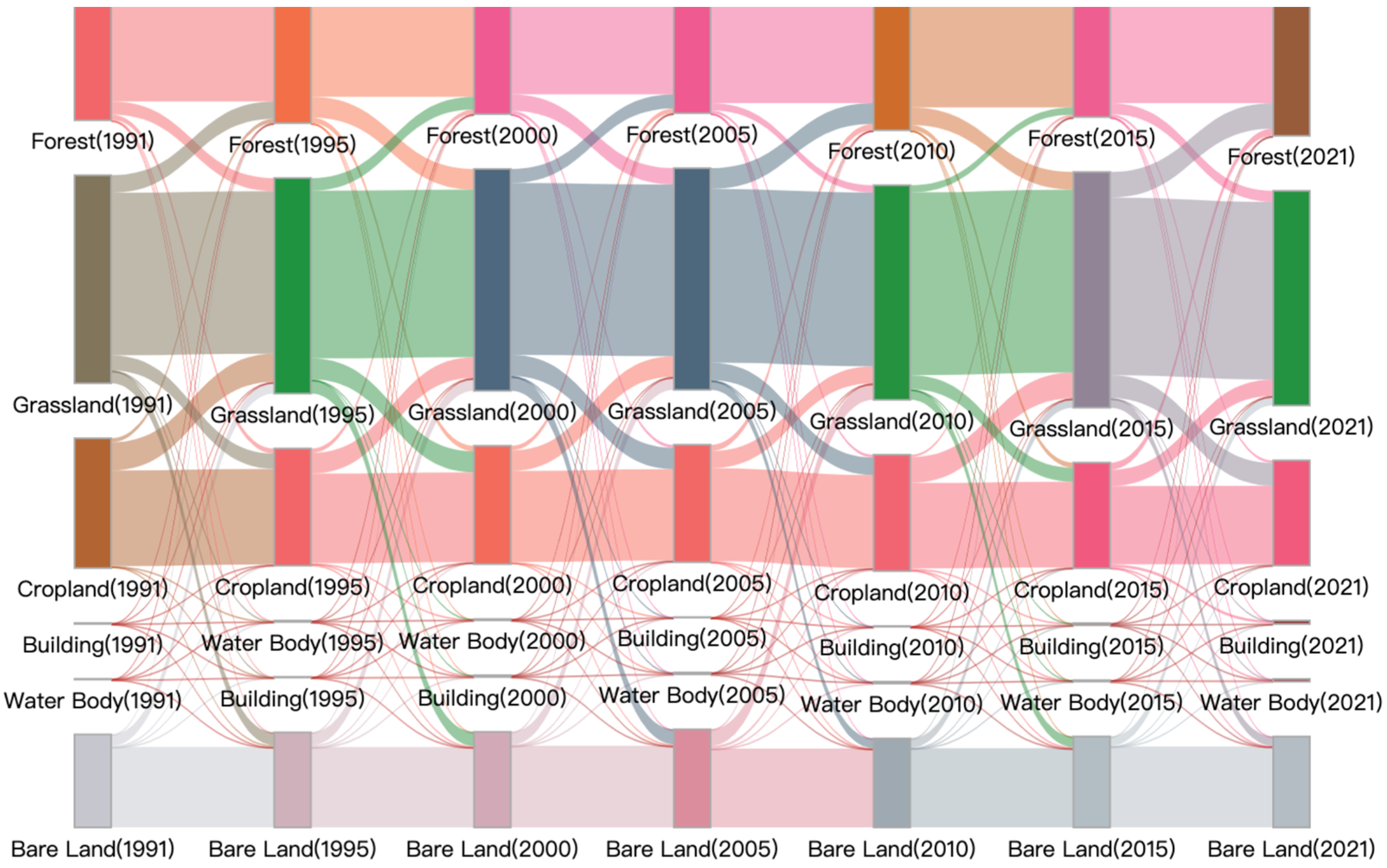
The areas of different land use types in 1991, 1995, 2000, 2005, 2010, 2015, and 2021 were extracted and analyzed. Land use transition information was visualized using Sankey diagrams (Figure 6). It shows that forest area increased from 366,800 km2 in 1991 to 415,600 km2 in 2021, mainly converted from grassland. The area of grassland increased from 652,000 km2 in 1991 to 672,700 km2 in 2021, primarily converted from cropland. Since the implementation of China’s Grain for Green policy in 1999, the area of cropland decreased from 370,790 km² in 1999 to 329,500 km² in 2021, mainly transferred to grassland, with the largest transfer of 64,560 km² occurring from 2010 to 2015. The area of water body increased from 2053 km2 in 1991 to 8217 km2 in 2020. Overall, the ecological conditions in North China have continuously improved.

4.2. Spatiotemporal Dynamics of Ecosystem Service Values in North China

(1) Overall assessment
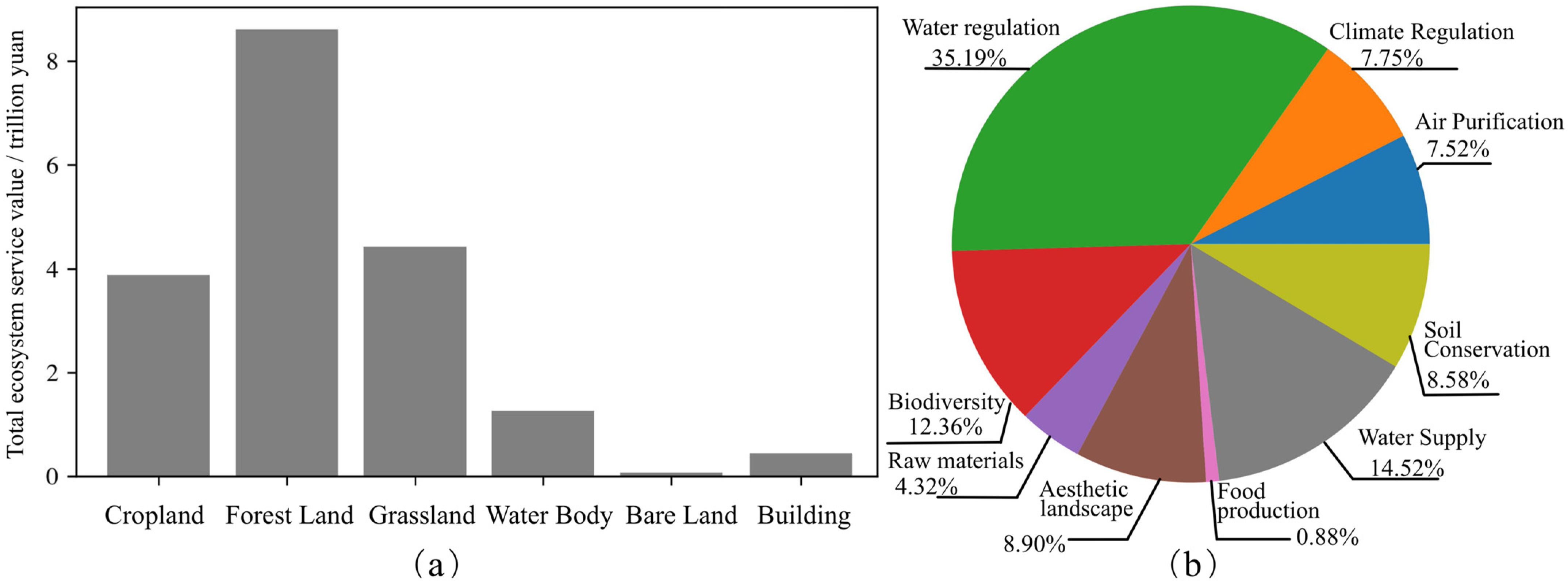
The total values of different types of ecosystem service values (ESV) in North China averaged CNY 18.23 trillion from 1991 to 2021 (Figure 7). Among ecosystem types, forests had the highest ESV at CNY 8.61 trillion, accounting for 45.84% of the total. Grasslands and croplands followed with 23.50% and 20.64% of the total value. Water bodies, buildings, and bare land had relatively small proportions of 6.73%, 2.93%, and 0.36% due to their limited area, with ESV of water at CNY 1.26 trillion. For ecosystem service functions, regulating services were most valuable, including water flow regulation (CNY 2.37 trillion, 35.19% of the total), climate regulation (CNY 0.52 trillion, 7.75% of the total), and air purification (CNY 0.51 trillion, 7.52% of the total). Soil conservation, biodiversity maintenance, and aesthetic landscape followed at around 29.84% of the total value. Other services had relatively low values at 5.20% of the total.
(2) Spatial variations
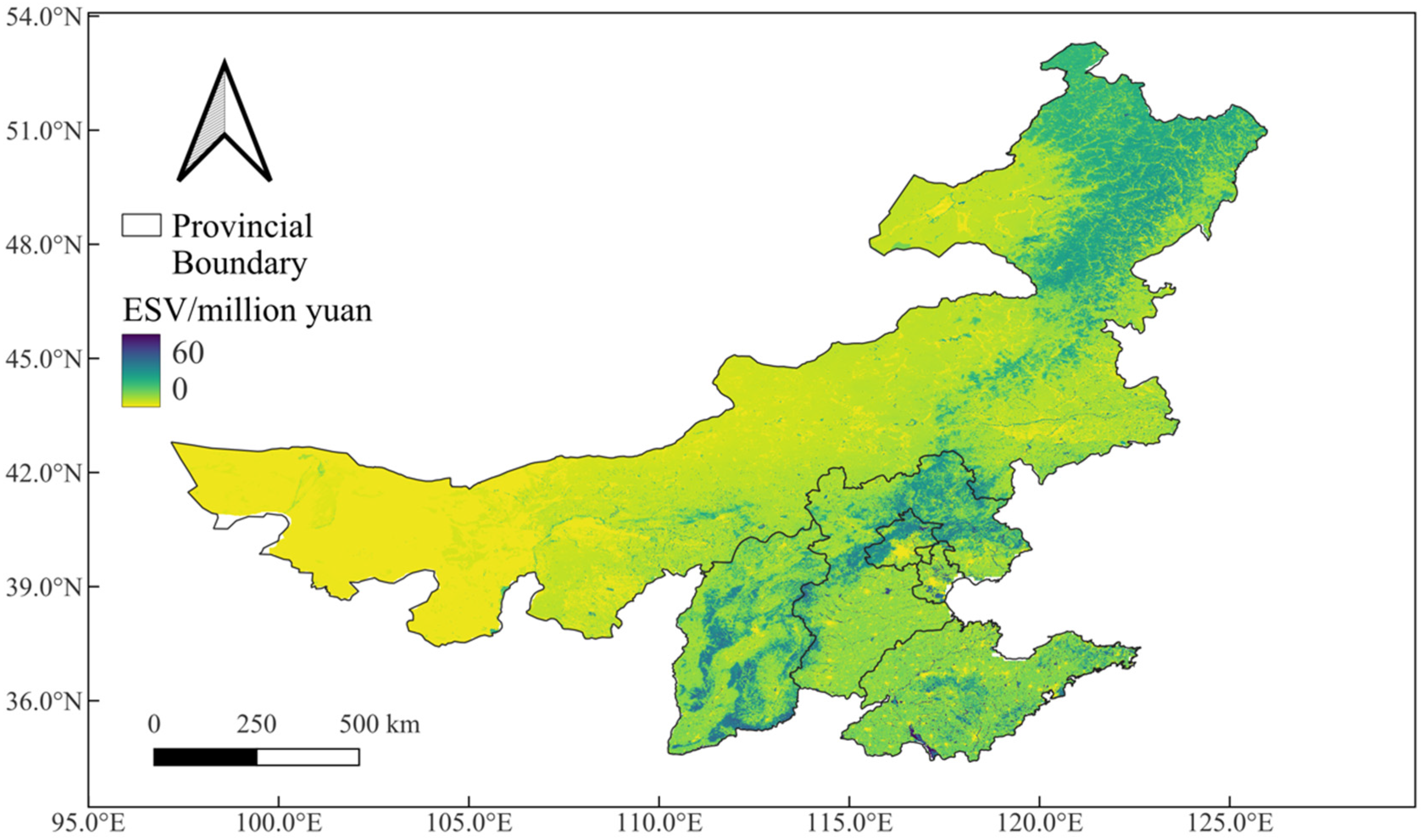
The spatial distribution of mean ecosystem service values in North China generally decreased from southeast to northwest, consistent with NDVI and precipitation patterns (Figure 8). Among the six provinces, Inner Mongolia had the highest ESV (54.24%), followed by Hebei (16.18%), Shanxi (14.69%), Shandong (11.98%), Beijing (1.98%), and Tianjin (0.93%). This pattern was influenced by the total ecosystem area and ESV per unit area in each province.
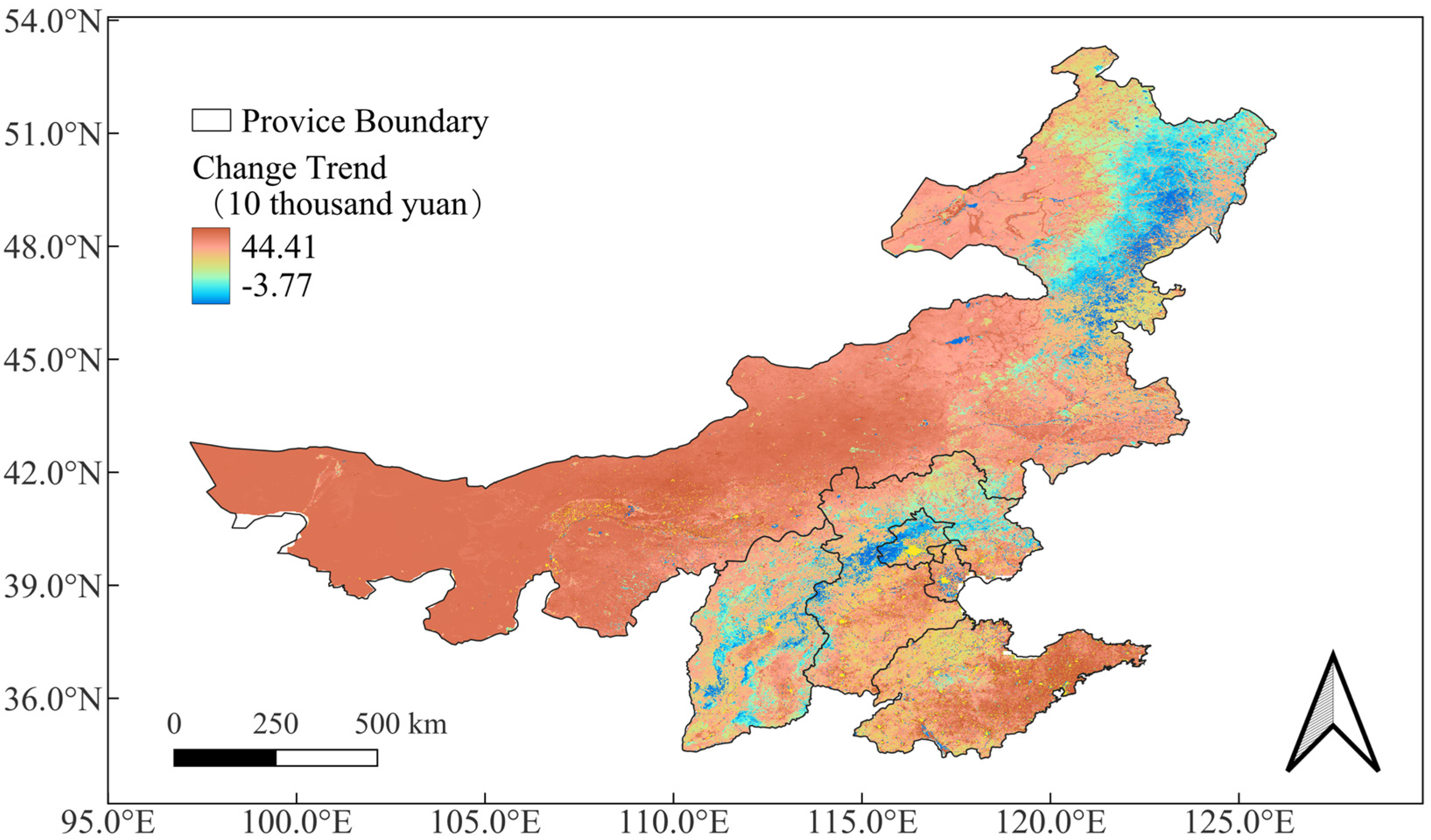
The interannual trends in ecosystem service value were heavily influenced by climate change and ecological engineering implementation. China has undertaken major programs like Grain for Green since 1999, effectively increasing vegetation coverage and regional ecosystem service values [2]. The spatial dynamics and significance test for total ESV in North China from 1991 to 2021 are shown in Figure 9. Figure 9 illustrates that areas with higher increases were concentrated in central Beijing and Hebei, while larger decreases occurred in eastern Shandong and central–west Inner Mongolia. Significance testing (Figure 10) revealed increasing ESV trends for most regions from 1991 to 2021, with significant and extremely significant increases accounting for 50.28% and 16.26% of the total area. ESV declines covered 30.57% of North China, with 30.34% and 0.24% showing significant and extremely significant decreases.
(3) Seasonal variations
ESVs were highest in August and decreased towards winter, except for building and bare land, which were temporally stable. The peak in summer coincides with the rainy season and peak plant growth (Figure 11). Water bodies reached maximum values of CNY 0.14, 0.18, and 0.11 trillion in July, August, and September, reflecting the influence of precipitation on its ESV. The seasonal distribution of ESV peaked in August and decreased towards winter, reflecting the influence of monsoonal climate and ecosystem growth cycles in the study area. In winter, low temperatures, scarce rainfall, and vegetation dormancy or mortality result in minimum NDVI and ESV. From winter to summer, rising temperatures and precipitation increase NDVI accumulation rates, enhancing ecological functions and ESV. From summer to winter, declining temperatures slow or halt biological growth, reducing ESV. These seasonal impacts are most pronounced for forests and grasslands, followed by croplands. The ESV of water bodies mainly depends on intra-annual rainfall distribution, peaking in July-August with high precipitation, indicating a higher per-unit-area ESV under favorable water and temperature conditions for vegetation growth, and vice versa.

4.3. Spatiotemporal Variation of Ecological Drought

(1) Spatial distribution
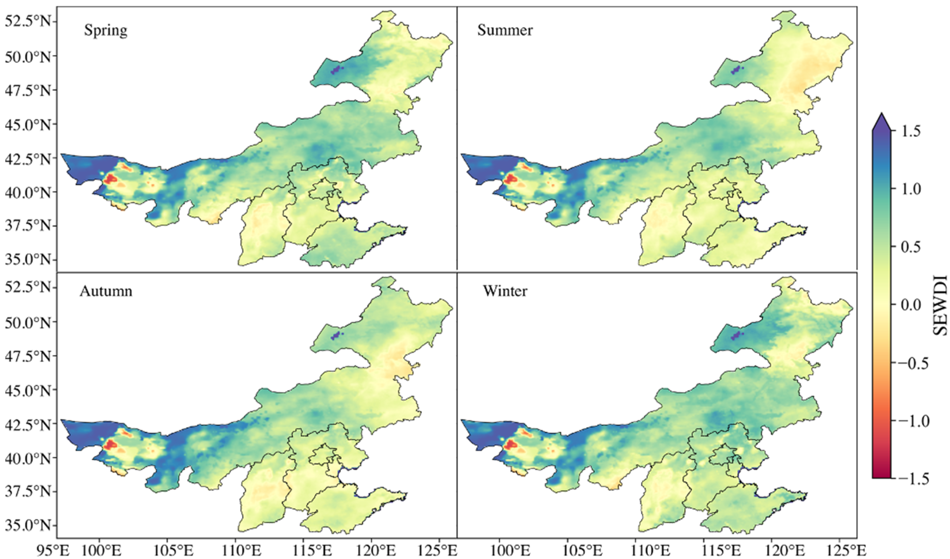
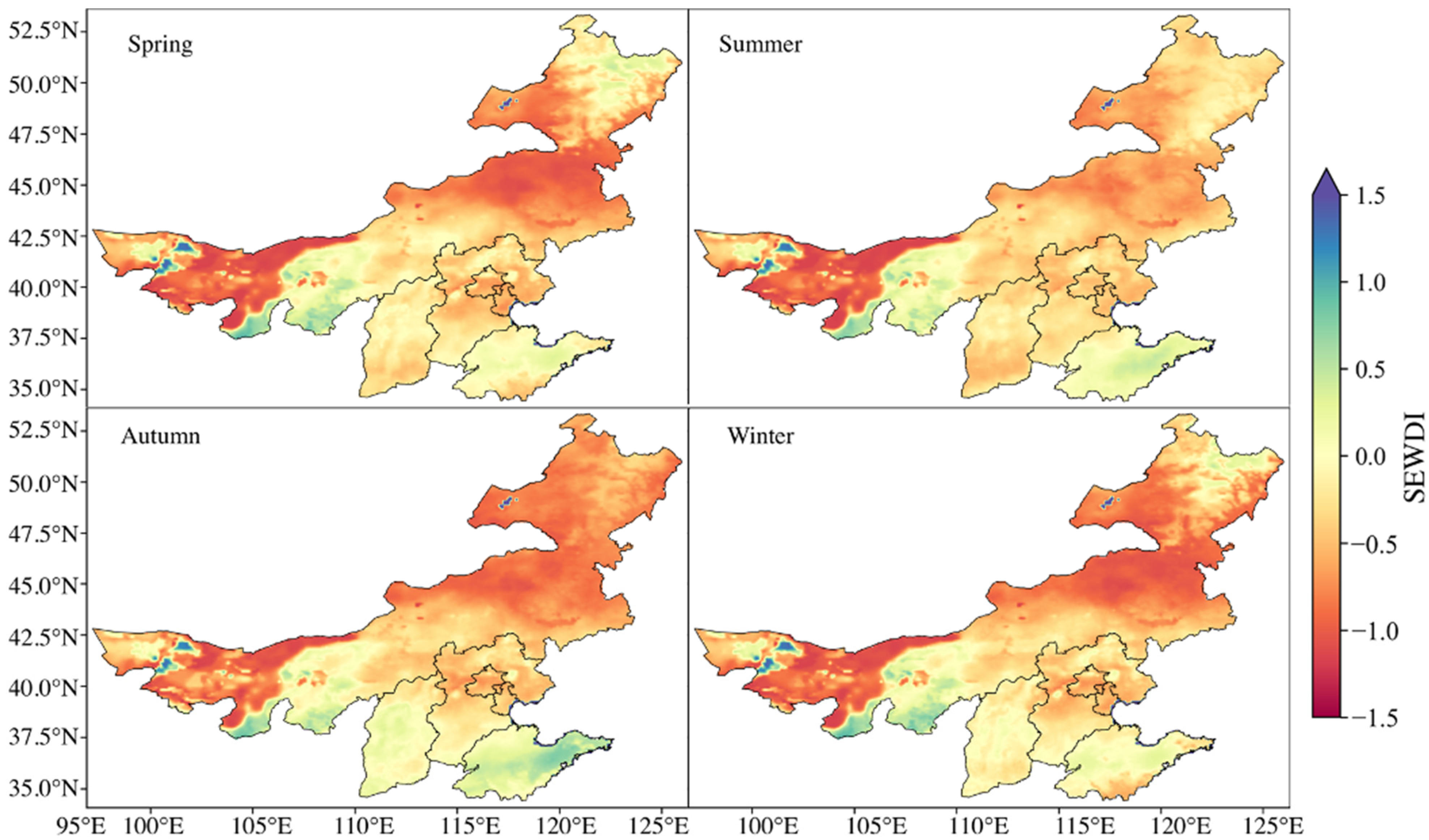
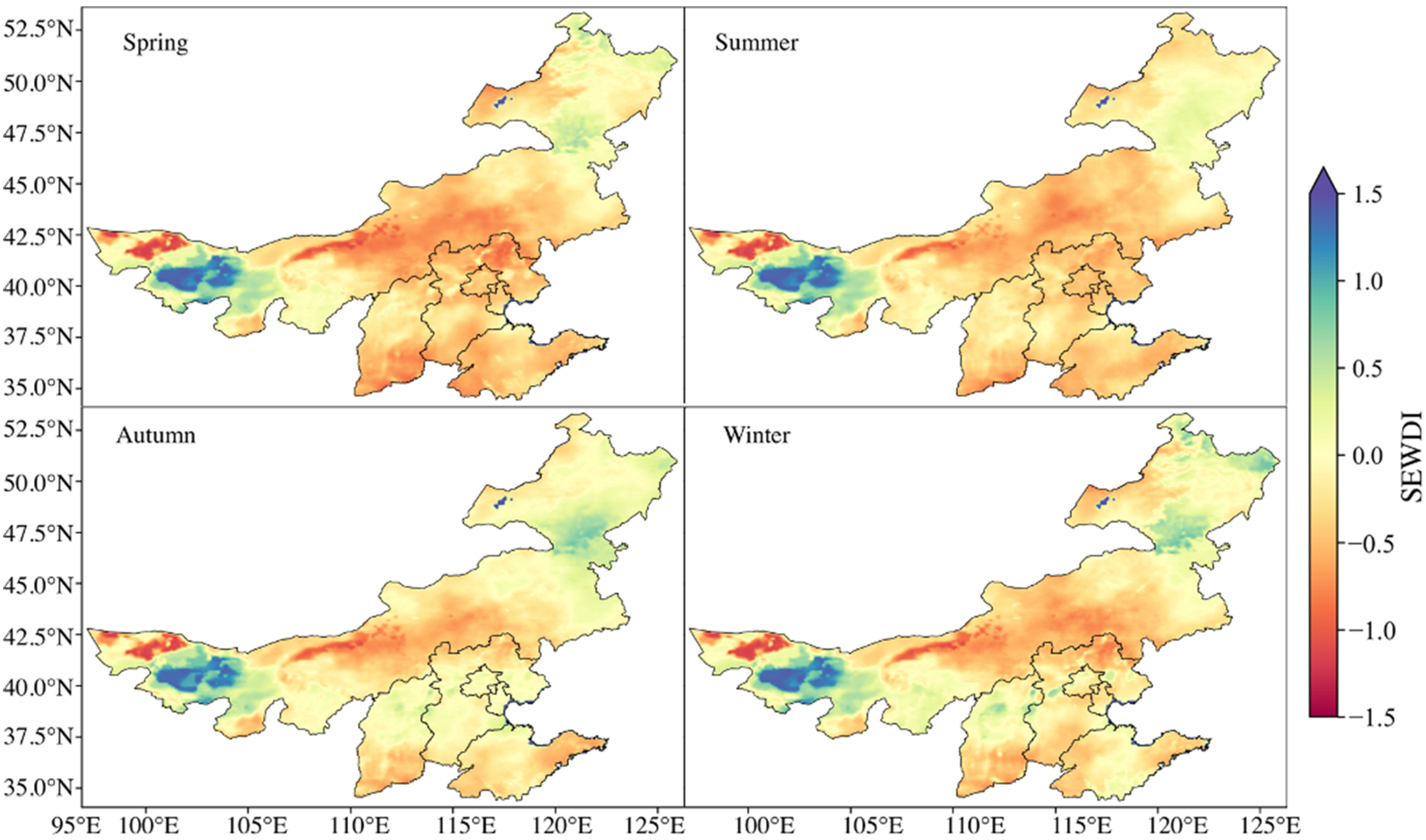
By calculating the ecological drought index, this study analyzed the spatiotemporal variation of ecological drought in spring, summer, autumn, and winter in North China during three periods from 1991 to 2021 (1991–2001, 2002–2011, and 2012–2021) (Figure 12, Figure 13 and Figure 14). The results show that 1991–2001 was a relatively wet period for the whole region; 2002–2011 was the most severe ecological drought phase in the past 30 years, especially in central and eastern Inner Mongolia; and there was some relief in 2012–2021.
(2) Temporal evolution of ecological drought
Figure 15 shows the temporal variation of SEWDI in North China from January 1991 to December 2021, presenting certain periodic characteristics. During 1991–2000, the SEWDI generally rose, and the proportion of drought impact area decreased; during 2000–2010, SEWDI fluctuated downward, and the proportion of drought impact area increased. It is important to note that, based on the classification standards of the Standardized Drought Index, a SEWDI value of less than -1.5 indicates a condition of serious drought. Several serious drought events with the largest intensity and duration since 1991 were identified in this period. It has been reported that North China suffered from a sustained drought event in 2002, water resources were tense in the Yellow River Basin, some areas were cut off, and agricultural, urban, and ecological water use was threatened [39]. In 2009, the most severe winter–spring consecutive drought occurred in North China since 1951, with the largest severity and impact area since 1982 [40]. Afterwards, ecological drought was relieved again during 2014–2021.
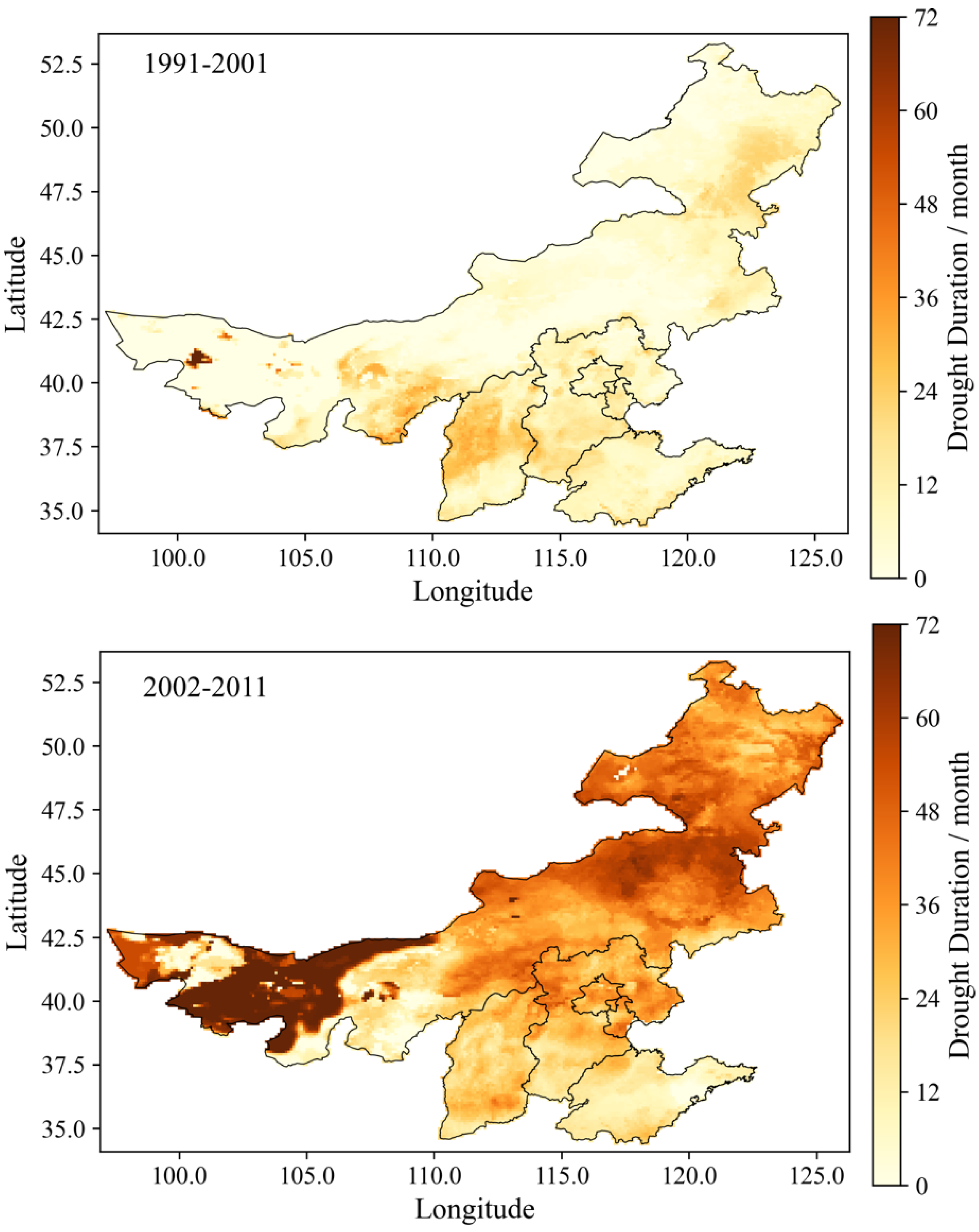
Figure 16 shows the spatial distribution of the total duration of all ecological drought events in North China during different stages. It can be seen that there was an increasing then decreasing trend during 1982–2021. The proportion of the area with a total duration greater than 25 months exceeded 50% after the 21st century, while it was only 4.9% before the 21st century. The total duration reached the maximum during 2002–2011, with the proportional area greater than 25 months up to 64.3%. Combined with Figure 11, Figure 12 and Figure 13, it can be seen that the long-duration and high-intensity ecological drought in North China during 2002–2011 was mainly distributed in most parts of Inner Mongolia, northern Hebei, Beijing, and Tianjin. During 2012–2021, ecological drought in Inner Mongolia, Hebei, and Shanxi alleviated, while Shandong still showed an intensifying trend.

4.4. Ecosystem Vulnerability Assessment

(1) Spatial distribution of ecosystem vulnerability
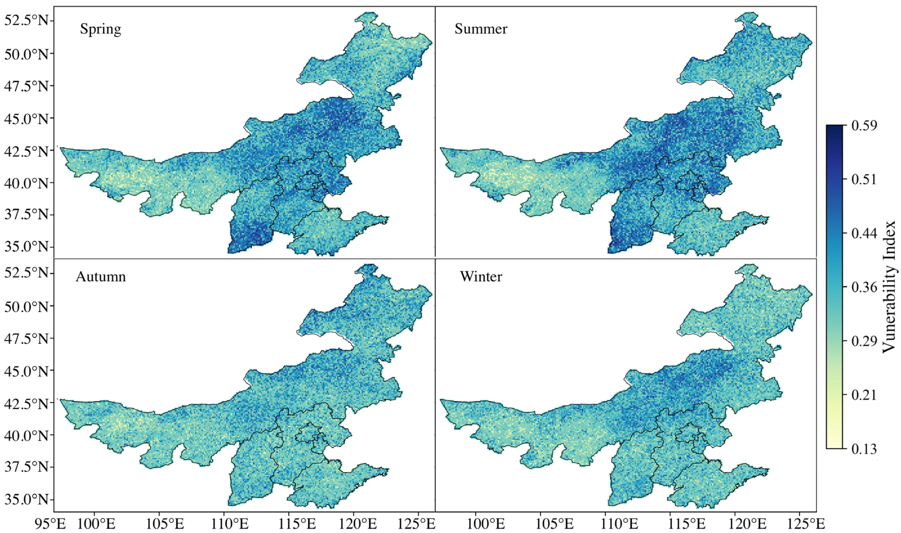
Figure 17 shows the vulnerability of ecosystems to drought in North China in spring, summer, autumn, and winter. Overall, the central region has a higher vulnerability, mainly distributed in central Inner Mongolia, northern Hebei, northern Shanxi, Beijing, and Tianjin. Seasonally, ecosystem vulnerability in North China is highest in autumn and lowest in winter, with mean vulnerability indices of 0.34, 0.37, 0.32, and 0.30 in spring, summer, autumn, and winter, respectively.
(2) Vulnerability maps of forest, grassland, and water ecosystems
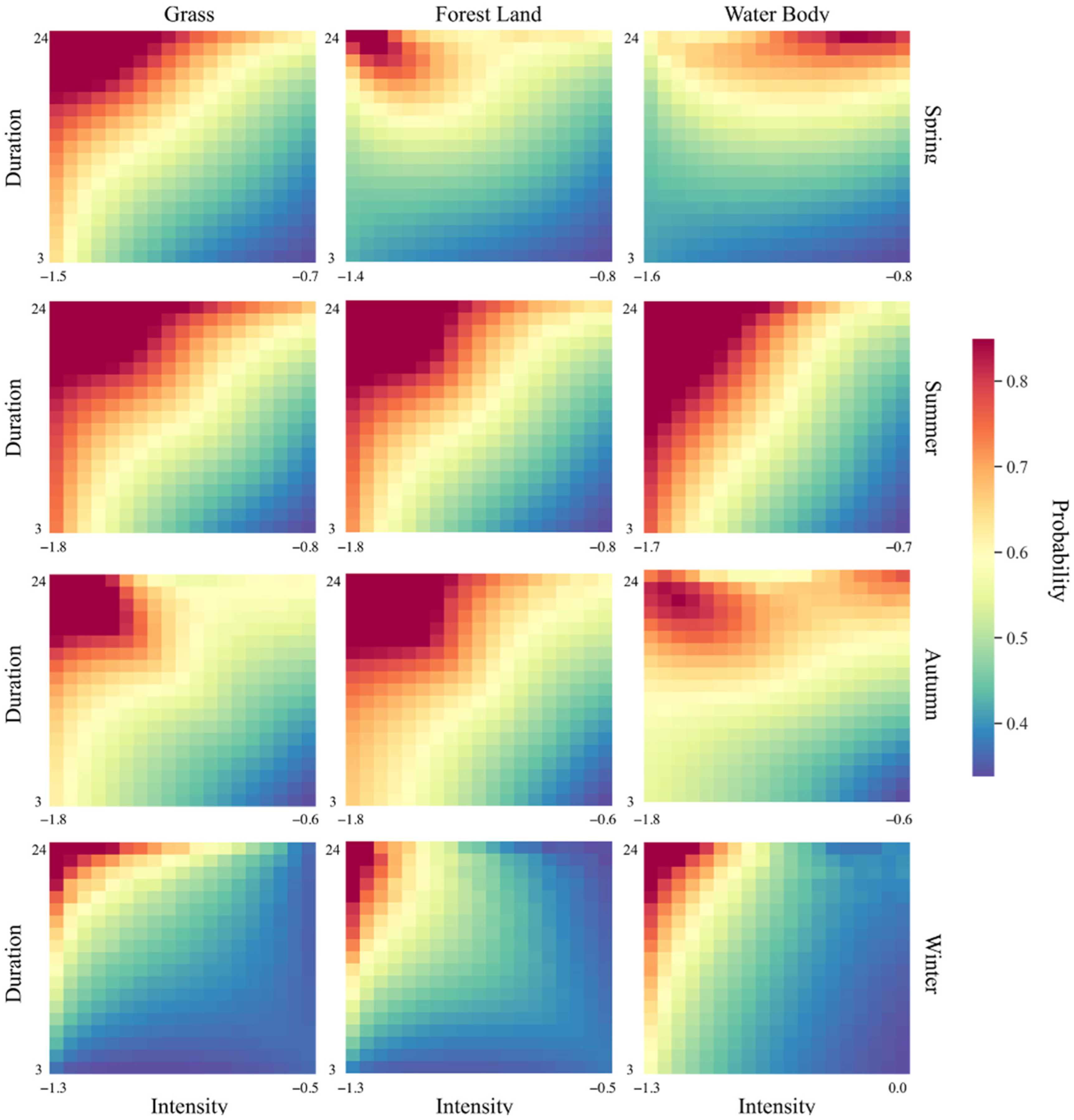
Figure 18 shows that vulnerability is higher in spring, summer, and autumn and lower in winter for both terrestrial and aquatic systems in North China. The phenomenon that forest vulnerability is lower than grassland is more pronounced. For example, for forests, when autumn drought intensity is −0.75 and drought area proportion is 45%, the vulnerability index is 0.79, while for grasslands under the same conditions, the vulnerability index is 0.91.

5. Discussion

5.1. Ecological Drought and Its Impact on ESV in North China

Over the past three decades, the climatic conditions in North China have demonstrated significant fluctuations, with alternating wet and dry periods. From 1991 to 2001, the region experienced relatively high precipitation, largely influenced by the Asian monsoon system, which played a critical role in regulating summer rainfall [41]. Moreover, the Pacific Interdecadal Oscillation (PDO) likely enhanced moisture availability during this period, contributing to wetter conditions [42]. In contrast, the period from 2002 to 2011 was marked by a severe ecological drought, particularly in central and eastern Inner Mongolia, driven by rising temperatures and decreasing precipitation [43]. The weakening of the Asian monsoon circulation further exacerbated these drought conditions [41], leading to significant water stress that negatively impacted vegetation cover [44]. Following this drought phase, the period from 2012 to 2021 saw a partial recovery, as increased precipitation and reduced temperature extremes contributed to the gradual restoration of vegetation and ecosystem health [45].
It is important to distinguish between ecological drought and ecosystem service value (ESV). Ecological drought is primarily driven by climatic factors such as changes in precipitation and temperature [46], whereas ESV encompasses a broader range of ecosystem services, including food production, water regulation, climate regulation, and more. While the Grain for Green program, initiated in 1999, aimed to enhance ESV by promoting reforestation and ecological restoration, the observed reduction in ESV during the period after 1999, particularly in 2002 to 2011, can be explained by the severe ecological drought experienced in North China during this time [47]. Inner Mongolia and other parts of North China faced significant declines in precipitation and rising temperatures, which led to reduced vegetation cover and, consequently, lower ESV [43]. This highlights how climatic factors can have a more immediate and pronounced impact on ecological conditions, even when long-term restoration programs like Grain for Green are underway.

5.2. Drought Vulnerability across Vegetation Types and Seasonal Variations

The differences in drought vulnerability between forests and grasslands are mainly influenced by their own drought-resistance characteristics [16,18,20,48]. The forest system has deep and robust root systems that can better absorb and utilize soil moisture. In contrast, grasslands have shallow root systems that can only absorb surface soil moisture, thus being more sensitive to droughts [49,50]. In addition, the canopy and leaves in the forest system can effectively block sunlight and reduce evaporation to better conserve soil moisture. In contrast, low-profile grasslands fail to provide adequate shade, leading to heightened soil moisture evaporation and increased drought susceptibility during summer and autumn [51]. Moreover, the diversity of vegetation types and species within forest ecosystems contributes to their resilience and adaptability, whereas the homogeneity of vegetation and lower species diversity in grasslands amplify their vulnerability [52]. In summary, the breadth of services provided by forests acts as a buffer, whereas grasslands are more susceptible due to narrower service capacities.
The seasonal differences in aquatic ecosystem vulnerability are mainly influenced by intra-annual climate variations [53]. Summer and autumn are more sensitive to droughts, with vulnerability varying greatly with changes in drought intensity and duration, while droughts have less impact on aquatic ecosystems in winter and spring. There are two main reasons: First, precipitation is lower in winter and spring, water storage in reservoirs and lakes is lower, and water content is lower, so the response is insignificant when droughts occur [54]. Second, the dormancy of most plant species during winter and spring entails slowed growth and reduced water demand, thus weakening the response to droughts. In contrast, plant growth is robust and water demand is high during summer and autumn, causing plants in aquatic ecosystems to be easily impacted by droughts and resulting in heightened vulnerability [55]. Moreover, heightened provisioning and cultural service demands, cascading effects on regulating services, and greater stresses to aquatic habitats and biodiversity result in summer/autumn droughts disproportionately impacting ecosystem service values, compared to spring/winter [56].

6. Conclusions

This study introduced a novel approach to assess the spatiotemporal dynamics of ecosystem service values (ESV) and ecological drought vulnerability in North China from 1991 to 2021. Significant land use changes were observed, with increases in forest and grassland and decreases in cropland, aligning with China’s ecological restoration programs and contributing to rising ESV, particularly in Beijing and Hebei. ESV showed clear seasonal patterns, peaking in summer, and spatial patterns decreasing from southeast to northwest, driven by climate and vegetation. Ecological drought, particularly severe between 2002 and 2011 in Inner Mongolia, Beijing, and Tianjin, led to increased drought duration and frequency, resulting in declining ESV. Grasslands were found to be more sensitive to drought than forests, and vulnerability was higher in summer and autumn. However, this study has limitations, including the potential for missed localized impacts due to dataset resolution and the focus on vegetation-related services. Future research should incorporate higher-resolution data, a broader range of ecosystem services, and socio–economic factors such as water management policies. Overall, this integrated approach offers valuable insights for drought resilience planning and sustainable development in North China.

Author Contributions

Conceptualization, T.J. and Y.Q.; methodology, T.J., K.F. and G.Z.; validation, Y.Q.; formal analysis, Y.H. and L.J.; investigation, X.Z., L.J. and Y.H.; data curation, G.Z. and Y.H.; writing—original draft preparation, T.J.; writing—review and editing, T.J., Y.Q. and Y.H.; visualization, T.J.; supervision, Y.Q.; project administration, Y.Q.; funding acquisition, Y.Q. All authors have read and agreed to the published version of the manuscript.

Funding

This study was financially supported by the national key research and development program of China funded project (2023YFC3006604), the Special Project of Basic Scientific Research Business Expenses of China Academy of Water Resources and Hydropower Research (JZ110145B0022024), 2024 Public Business Expenses of Research Center on Flood and Drought Reduction Center (GY2401), Key Research and Development Program of Jiangxi Province (20232BBG70029-1), and ‘Science and Technology + Water Resources’ Joint Plan Project of Jiangxi Province (2022KSG01002-1).

Data Availability Statement

This study utilized three main types of datasets—geospatial data, topographic data, and vegetation data. The geospatial data were obtained from Google Earth Engine (GEE), including Landsat 5 TM, Landsat 7 ETM+, and Landsat 8 OLI imagery. Specifically, the Landsat 5 TM images spanned from 1984 to 2011 with a spatial resolution of 30 m. Landsat 7 ETM+ images were from 1999 to the present with a spatial resolution of 30 m. And Landsat 8 OLI images covered 2013 to the present with a spatial resolution of 30 m. The topographic data were the SRTM digital elevation model (DEM) provided by NASA/USGS/JPL Caltech, which had a spatial resolution of 90 m. Vegetation data consisted of the Normalized Difference Vegetation Index (NDVI), which was obtained from composite Landsat NDVI datasets downloaded from http://www.gis5g.com/data/zbsj/NDVI (accessed on 14 June 2024), with a spatial resolution of 30 m, ensuring consistency across the study period. Meteorological datasets, including monthly precipitation and monthly temperatures spanning from 1979 to present with a spatial resolution of 0.25° × 0.25°, were derived from the ERA-Interim reanalysis dataset produced by the European Center for Medium-Range Weather Forecasts (ECMWF). Agricultural data, including food production and yield prices, were sourced from the National Bureau of Statistics of China, available through their publicly accessible database: https://data.stats.gov.cn/ (accessed on 3 June 2024).

Conflicts of Interest

The authors declare no conflicts of interest.

References

  1. Shin, H. A critical review of robot research and future research opportunities: Adopting a service ecosystem perspective. Int. J. Contemp. Hosp. Manag. 2022, 34, 2337–2358. [Google Scholar] [CrossRef]
  2. Lin, L.; Wei, X.; Luo, P.; Wang, S.; Kong, D.; Yang, J. Ecological Security Patterns at Different Spatial Scales on the Loess Plateau. Remote Sens. 2023, 15, 1011. [Google Scholar] [CrossRef]
  3. Costanza, R. Valuing natural capital and ecosystem services toward the goals of efficiency, fairness, and sustainability. Ecosyst. Serv. 2020, 43, 101096. [Google Scholar] [CrossRef]
  4. Hasan, S.; Zhen, L.; Miah, M.; Ahamed, T.; Samie, A. Impact of land use change on ecosystem services: A review. Environ. Dev. 2020, 34, 100527. [Google Scholar] [CrossRef]
  5. Pan, F.; Shu, N.; Wan, Q.; Huang, Q. Land Use Function Transition and Associated Ecosystem Service Value Effects Based on Production-Living-Ecological Space: A Case Study in the Three Gorges Reservoir Area. Land 2023, 12, 391. [Google Scholar] [CrossRef]
  6. Xie, L.; Wang, H.; Liu, S. The ecosystem service values simulation and driving force analysis based on land use/land cover: A case study in inland rivers in arid areas of the Aksu River Basin, China. Ecol. Indic. 2022, 138, 108828. [Google Scholar] [CrossRef]
  7. Yu, H.; Yang, J.; Sun, D.; Li, T.; Liu, Y. Spatial Responses of Ecosystem Service Value during the Development of Urban Agglomerations. Land 2022, 11, 165. [Google Scholar] [CrossRef]
  8. Ding, M.; Liu, W.; Xiao, L.; Zhong, F.; Lu, N.; Zhang, J.; Zhang, Z.; Xu, X.; Wang, K. Construction and optimization strategy of ecological security pattern in a rapidly urbanizing region: A case study in central-south China. Ecol. Indic. 2022, 136, 108604. [Google Scholar] [CrossRef]
  9. Zhu, S.; Huang, J.; Zhao, Y. Coupling coordination analysis of ecosystem services and urban development of resource-based cities: A case study of Tangshan city. Ecol. Indic. 2022, 136, 108706. [Google Scholar] [CrossRef]
  10. Peng, K.; Jiang, W.; Ling, Z.; Hou, P.; Deng, Y. Evaluating the potential impacts of land use changes on ecosystem service value under multiple scenarios in support of SDG reporting: A case study of the Wuhan urban agglomeration. J. Clean. Prod. 2021, 307, 127321. [Google Scholar] [CrossRef]
  11. Jiang, Y.; Guan, D.; He, X.; Yin, B.; Zhou, L.; Sun, L.; Huang, D.; Li, Z.; Zhang, Y. Quantification of the coupling relationship between ecological compensation and ecosystem services in the Yangtze River Economic Belt, China. Land Use Policy 2022, 114, 105995. [Google Scholar] [CrossRef]
  12. Pan, N.; Guan, Q.; Wang, Q.; Sun, Y.; Li, H.; Ma, Y. Spatial Differentiation and Driving Mechanisms in Ecosystem Service Value of Arid Region:A case study in the middle and lower reaches of Shule River Basin, NW China. J. Clean. Prod. 2021, 319, 128718. [Google Scholar] [CrossRef]
  13. Wu, J.; Wang, G.; Chen, W.; Pan, S.; Zeng, J. Terrain gradient variations in the ecosystem services value of the Qinghai-Tibet Plateau, China. Glob. Ecol. Conserv. 2022, 34, e02008. [Google Scholar] [CrossRef]
  14. Liang, J.; Xie, Y.; Sha, Z.; Zhou, A. Modeling urban growth sustainability in the cloud by augmenting Google Earth Engine (GEE). Comput. Environ. Urban Syst. 2020, 84, 101542. [Google Scholar] [CrossRef]
  15. Ma, S.; Huang, J.; Chai, Y. Proposing a GEE-Based Spatiotemporally Adjusted Value Transfer Method to Assess Land-Use Changes and Their Impacts on Ecosystem Service Values in the Shenyang Metropolitan Area. Sustainability 2021, 13, 12694. [Google Scholar] [CrossRef]
  16. Fathi-Taperasht, A.; Shafizadeh-Moghadam, H.; Sadian, A.; Xu, T.; Nikoo, M.R. Drought-induced vulnerability and resilience of different land use types using time series of MODIS-based indices. Int. J. Disaster Risk Reduct. 2023, 91, 103703. [Google Scholar] [CrossRef]
  17. Li, Y.; Zhang, W.; Schwalm, C.R.; Gentine, P.; Smith, W.K.; Ciais, P.; Kimball, J.S.; Gazol, A.; Kannenberg, S.A.; Chen, A.; et al. Widespread spring phenology effects on drought recovery of Northern Hemisphere ecosystems. Nat. Clim. Chang. 2023, 13, 182–188. [Google Scholar] [CrossRef]
  18. Liu, Y.; You, C.; Zhang, Y.; Chen, S.; Zhang, Z.; Li, J.; Wu, Y. Resistance and resilience of grasslands to drought detected by SIF in inner Mongolia, China. Agric. For. Meteorol. 2021, 308–309, 108567. [Google Scholar] [CrossRef]
  19. Machado-Silva, F.; Peres, L.F.; Gouveia, C.M.; Enrich-Prast, A.; Peixoto, R.B.; Pereira, J.M.C.; Marotta, H.; Fernandes, P.J.F.; Libonati, R. Drought Resilience Debt Drives NPP Decline in the Amazon Forest. Global Biogeochem. Cycles 2021, 35, e2021GB007004. [Google Scholar] [CrossRef]
  20. Xu, C.; Ke, Y.; Zhou, W.; Luo, W.; Ma, W.; Song, L.; Smith, M.D.; Hoover, D.L.; Wilcox, K.R.; Fu, W.; et al. Resistance and resilience of a semi-arid grassland to multi-year extreme drought. Ecol. Indic. 2021, 131, 108139. [Google Scholar] [CrossRef]
  21. Yao, Y.; Fu, B.; Liu, Y.; Li, Y.; Wang, S.; Zhan, T.; Wang, Y.; Gao, D. Evaluation of ecosystem resilience to drought based on drought intensity and recovery time. Agric. For. Meteorol. 2022, 314, 108809. [Google Scholar] [CrossRef]
  22. Liu, X.; Zhu, X.; Pan, Y.; Bai, J.; Li, S. Performance of different drought indices for agriculture drought in the North China Plain. J. Arid Land 2018, 10, 507–516. [Google Scholar] [CrossRef]
  23. Cai, X.; Zhang, W.; Fang, X.; Zhang, Q.; Zhang, C.; Chen, D.; Cheng, C.; Fan, W.; Yu, Y. Identification of Regional Drought Processes in North China Using MCI Analysis. Land 2021, 10, 1390. [Google Scholar] [CrossRef]
  24. Jarvis, A.; Reuter, H.I.; Nelson, A.; Guevara, E. Hole-Filled SRTM for the Globe Version 4. CGIAR-CSI SRTM 90 m. 2008. Available online: https://csidotinfo.wordpress.com/data/srtm-90m-digital-elevation-database-v4-1/ (accessed on 13 June 2024).
  25. Muñoz Sabater, J. ERA5-Land Monthly Averaged Data from 1981 to Present. Copernicus Climate Change Service (C3S) Climate Data Store (CDS). 2019. Available online: https://cds.climate.copernicus.eu/datasets/reanalysis-era5-land-monthly-means?tab=overview (accessed on 18 November 2022).
  26. Cao, Y.; Kong, L.; Zhang, L.; Ouyang, Z. The balance between economic development and ecosystem service value in the process of land urbanization: A case study of China’s land urbanization from 2000 to 2015. Land Use Policy 2021, 108, 105536. [Google Scholar] [CrossRef]
  27. Xie, G.; Zhang, C.; Zhen, L.; Zhang, L. Dynamic changes in the value of China’s ecosystem services. Ecosyst. Serv. 2017, 26, 146–154. [Google Scholar] [CrossRef]
  28. Yin, C.; He, Q.; Xie, P.; Liu, Y.; Zhang, Y.; Chen, W.; Bi, Q. Spatiotemporal variation of the ecosystem service value in China based on surface area. Ecol. Indic. 2023, 148, 110067. [Google Scholar] [CrossRef]
  29. Gao, F.; Cui, J.; Zhang, S.; Xin, X.; Zhang, S.; Zhou, J.; Zhang, Y. Spatio-Temporal distribution and driving factors of ecosystem service value in a fragile hilly area of North China. Land 2022, 11, 2242. [Google Scholar] [CrossRef]
  30. Xu, D.; Ding, X. Assessing the impact of desertification dynamics on regional ecosystem service value in North China from 1981 to 2010. Ecosyst. Serv. 2018, 30, 172–180. [Google Scholar] [CrossRef]
  31. Chi, D.; Wang, H.; Li, X.; Liu, H.; Li, X. Estimation of the ecological water requirement for natural vegetation in the Ergune River basin in Northeastern China from 2001 to 2014. Ecol. Indic. 2018, 92, 141–150. [Google Scholar] [CrossRef]
  32. O’Connor, R.C.; Germino, M.J.; Barnard, D.M.; Andrews, C.M.; Bradford, J.B.; Pilliod, D.S.; Arkle, R.S.; Shriver, R.K. Small-scale water deficits after wildfires create long-lasting ecological impacts. Environ. Res. Lett. 2020, 15, 044001. [Google Scholar] [CrossRef]
  33. Vicente-Serrano, S.M.; Miralles, D.G.; Domínguez-Castro, F.; Azorin-Molina, C.; Kenawy, A.E.; McVicar, T.R.; Tomás-Burguera, M.; Beguería, S.; Maneta, M.; Peña-Gallardo, M. Global Assessment of the Standardized Evapotranspiration Deficit Index (SEDI) for Drought Analysis and Monitoring. J. Clim. 2018, 31, 5371–5393. [Google Scholar] [CrossRef]
  34. Deb, P.; Kiem, A.S.; Willgoose, G. A linked surface water-groundwater modelling approach to more realistically simulate rainfall-runoff non-stationarity in semi-arid regions. J. Hydrol. 2019, 575, 273–291. [Google Scholar] [CrossRef]
  35. Jiang, T.; Su, X.; Singh, V.P.; Zhang, G. A novel index for ecological drought monitoring based on ecological water deficit. Ecol. Indic. 2021, 129, 107804. [Google Scholar] [CrossRef]
  36. Zamani Losgedaragh, S.; Rahimzadegan, M. Evaluation of SEBS, SEBAL, and METRIC models in estimation of the evaporation from the freshwater lakes (Case study: Amirkabir dam, Iran). J. Hydrol. 2018, 561, 523–531. [Google Scholar] [CrossRef]
  37. McKee, T.B.; Doesken, N.J.; Kleist, J. The relationship of drought frequency and duration to time scales. In Proceedings of the 8th Conference on Applied Climatology, Anaheim, CA, USA, 17–22 January 1993; pp. 179–183. [Google Scholar]
  38. Mesbahzadeh, T.; Mirakbari, M.; Mohseni Saravi, M.; Soleimani Sardoo, F.; Miglietta, M.M. Meteorological drought analysis using copula theory and drought indicators under climate change scenarios (RCP). Meteorol. Appl. 2020, 27, e1856. [Google Scholar] [CrossRef]
  39. Zou, X.; Zhai, P.; Zhang, Q. Variations in droughts over China: 1951–2003. Geophys. Res. Lett. 2005, 32, L04707. [Google Scholar] [CrossRef]
  40. Shao, D.; Chen, S.; Tan, X.; Gu, W. Drought characteristics over China during 1980–2015. Int. J. Climatol. 2018, 38, 3532–3545. [Google Scholar] [CrossRef]
  41. Huang, J.; Xue, Y.; Sun, S.; Zhang, J. Spatial and temporal variability of drought during 1960–2012 in inner mongolia, north china. Quat. Int. 2015, 355, 134–144. [Google Scholar] [CrossRef]
  42. Ma, Z.; Sun, P.; Zhang, Q.; Hu, Y.; Jiang, W. Characterization and evaluation of MODIS-derived crop water stress index (CWSI) for monitoring drought from 2001 to 2017 over inner mongolia. Sustainability 2021, 13, 916. [Google Scholar] [CrossRef]
  43. Kang, Y.; Guo, E.; Wang, Y.; Bao, Y.; Mandula, N. Monitoring vegetation change and its potential drivers in inner mongolia from 2000 to 2019. Remote Sens. 2021, 13, 3357. [Google Scholar] [CrossRef]
  44. Gong, Z.; Kawamura, K.; Ishikawa, N.; Goto, M.; Wulan, T.; Alateng, D.; Yin, T.; Ito, Y. MODIS normalized difference vegetation index (NDVI) and vegetation phenology dynamics in the inner mongolia grassland. Solid Earth 2015, 6, 1185–1194. [Google Scholar] [CrossRef]
  45. An, Q.; He, H.; Nie, Q.; Cui, Y.; Gao, J.; Wei, C.; Xie, X.; You, J. Spatial and temporal variations of drought in inner mongolia, china. Water 2020, 12, 1715. [Google Scholar] [CrossRef]
  46. Jiang, T.; Su, X.; Zhang, G.; Zhang, T.; Wu, H. Estimating propagation probability from meteorological to ecological droughts using a hybrid machine learning copula method. Hydrol. Earth Syst. Sci. 2023, 27, 559–576. [Google Scholar] [CrossRef]
  47. Wu, Z.; Wu, J.; He, B.; Liu, J.; Wang, Q.; Zhang, H.; Liu, Y. Drought offset ecological restoration program-induced increase in vegetation activity in the beijing-tianjin sand source region, china. Environ. Sci. Technol. 2014, 48, 12108–12117. [Google Scholar] [CrossRef] [PubMed]
  48. Huang, W.; Wang, W.; Cao, M.; Fu, G.; Xia, J.; Wang, Z.; Li, J. Local climate and biodiversity affect the stability of China’s grasslands in response to drought. Sci. Total Environ. 2021, 768, 145482. [Google Scholar] [CrossRef]
  49. Kowalski, K. Large-scale remote sensing analysis reveals an increasing coupling of grassland vitality to atmospheric water demand. Glob. Chang. Biol. 2024, 30, 5. [Google Scholar] [CrossRef]
  50. Lu, M. Heterogeneity in vegetation recovery rates post-flash droughts across different ecosystems. Environ. Res. Lett. 2024, 19, 074028. [Google Scholar] [CrossRef]
  51. Shinohara, Y.; Otsuki, K. Comparisons of soil-water content between a moso bamboo (Phyllostachys pubescens) forest and an evergreen broadleaved forest in western Japan. Plant Species Biol. 2015, 30, 96–103. [Google Scholar] [CrossRef]
  52. Deng, J.; Yin, Y.; Zhu, W.; Zhou, Y. Variations in soil bacterial community diversity and structures among different revegetation types in the Baishilazi Nature Reserve. Front. Microbiol. 2018, 9, 02874. [Google Scholar] [CrossRef]
  53. Vicente-Serrano, S.M.; Quiring, S.M.; Peña-Gallardo, M.; Yuan, S.; Domínguez-Castro, F. A review of environmental droughts: Increased risk under global warming? Earth-Sci. Rev. 2020, 201, 102953. [Google Scholar] [CrossRef]
  54. Loon, A.F.V.; Tijdeman, E.; Wanders, N.; Lanen, H.V.; Teuling, A.J.; Uijlenhoet, R. How climate seasonality modifies drought duration and deficit. J. Geophys. Res. Atmos. 2014, 119, 4640–4656. [Google Scholar] [CrossRef]
  55. Saeidnia, F.; Majidi, M.M.; Mirlohi, A.; Soltan, S. Physiological and tolerance indices useful for drought tolerance selection in smooth bromegrass. Crop Sci. 2017, 57, 282–289. [Google Scholar] [CrossRef]
  56. Vogrinc, P.; Durso, A.; Winne, C.; Willson, J. Landscape-scale effects of supra-seasonal drought on semi-aquatic snake assemblages. Wetlands 2018, 38, 667–676. [Google Scholar] [CrossRef]
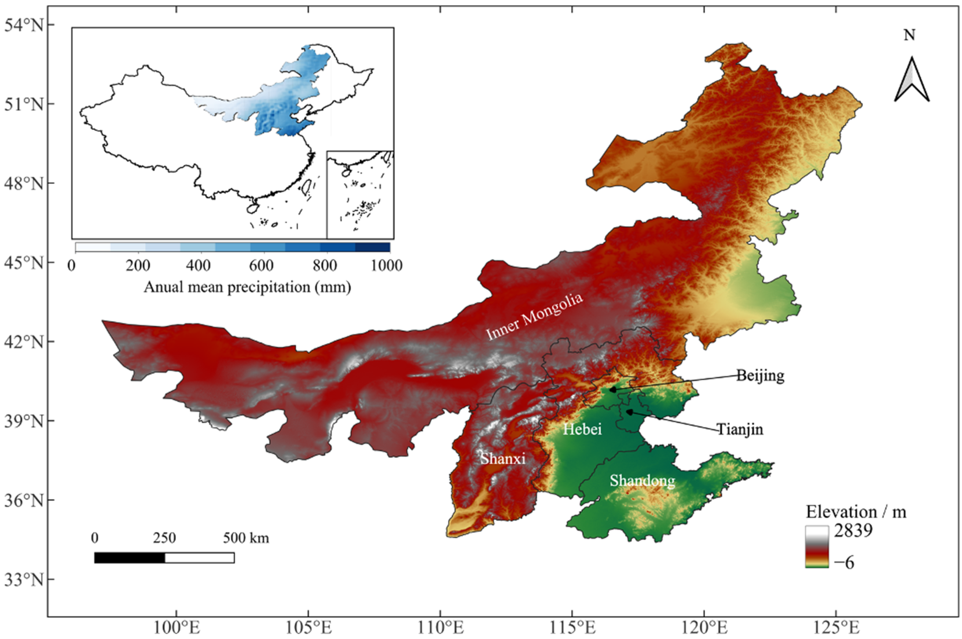
Figure 1. Location and elevation of study region.
Remotesensing 16 03733 g001
Figure 2. Technical process of the study.
Remotesensing 16 03733 g002
Figure 3. Schematic representation of time consistency evaluation.
Remotesensing 16 03733 g003
Figure 4. Spatial distribution of land use types in North China for typical years 1991, 2000, 2010, and 2020.
Remotesensing 16 03733 g004
Figure 5. Classification accuracy of land use types under three processing modes.
Remotesensing 16 03733 g005
Figure 6. Sankey diagram of land use changes in North China from 1991 to 2021.
Remotesensing 16 03733 g006
Figure 7. Ecosystem service values by (a) ecosystem type and (b) service function.
Remotesensing 16 03733 g007
Figure 8. Spatial distribution of mean ecosystem service values in North China, 1991–2021.
Remotesensing 16 03733 g008
Figure 9. Trends of total ecosystem service value changes in North China, 1991–2021.
Remotesensing 16 03733 g009
Figure 10. Significance test for total ecosystem service value changes in North China, 1991–2021.
Remotesensing 16 03733 g010
Figure 11. Seasonal variation of ecosystem service values in North China.
Remotesensing 16 03733 g011
Figure 12. Spatial distribution of mean SEWDI in North China in 1991–2001.
Remotesensing 16 03733 g012
Figure 13. Spatial distribution of mean SEWDI in North China in 2002–2011.
Remotesensing 16 03733 g013
Figure 14. Spatial distribution of mean SEWDI in North China in 2012–2021.
Remotesensing 16 03733 g014
Figure 15. Time series of monthly SEWDI and proportion of drought area in North China from Janurary 1991 to Decmember 2021.
Remotesensing 16 03733 g015
Figure 16. Spatial distribution of total duration of ecological drought in North China.
Remotesensing 16 03733 g016aRemotesensing 16 03733 g016b
Figure 17. Spatial distribution of ecosystem vulnerability in North China.
Remotesensing 16 03733 g017
Figure 18. Seasonal vulnerability heatmaps for different systems in North China.
Remotesensing 16 03733 g018
Table 1. Unit area ecosystem service value equivalent coefficients.
Service FunctionCroplandForest LandGrasslandWater BodyBuildingBare Land
Regulating ServicesAir purification0.53.50.8000
Climate regulation0.892.70.90.4600
Water regulation1.641.311.3118.200.01
Provisioning ServicesFood production10.10.30.100.01
Water supply0.63.20.820.400.03
Raw materials0.12.60.050.0100
Supporting ServicesSoil conservation1.463.91.950.0100.03
Biodiversity0.713.261.092.4900.34
Cultural ServicesAesthetic landscape0.011.280.044.341.120.01
Disclaimer/Publisher’s Note: The statements, opinions and data contained in all publications are solely those of the individual author(s) and contributor(s) and not of MDPI and/or the editor(s). MDPI and/or the editor(s) disclaim responsibility for any injury to people or property resulting from any ideas, methods, instructions or products referred to in the content.