Article

Estimating Vertical Distribution of Total Suspended Matter in Coastal Waters Using Remote-Sensing Approaches

by
Hailong Zhang
1,2,3,
Xin Ren
1,
Shengqiang Wang
1,3,*,
Xiaofan Li
1,
Deyong Sun
1,3 and
Lulu Wang
1
1
School of Marine Sciences, Nanjing University of Information Science & Technology, Nanjing 210044, China
2
Key Laboratory of Coastal Zone Exploitation and Protection, Ministry of Natural Resources, Nanjing 210017, China
3
Key Laboratory of Space Ocean Remote Sensing and Application, Ministry of Natural Resources, Beijing 100081, China
*
Author to whom correspondence should be addressed.
Remote Sens. 2024, 16(19), 3736; https://doi.org/10.3390/rs16193736
Submission received: 28 August 2024 / Revised: 4 October 2024 / Accepted: 5 October 2024 / Published: 8 October 2024

Abstract

:
The vertical distribution of the marine total suspended matter (TSM) concentration significantly influences marine material transport, sedimentation processes, and biogeochemical cycles. Traditional field observations are constrained by limited spatial and temporal coverage, necessitating the use of remote-sensing technology to comprehensively understand TSM variations over extensive areas and periods. This study proposes a remote-sensing approach to estimate the vertical distribution of TSM concentrations using MODIS satellite data, with the Bohai Sea and Yellow Sea (BSYS) as a case study. Extensive field measurements across various hydrological conditions and seasons enabled accurate reconstruction of in situ TSM vertical distributions from bio-optical parameters, including the attenuation coefficient, particle backscattering coefficient, particle size, and number concentration, achieving a determination coefficient of 0.90 and a mean absolute percentage error of 26.5%. In situ measurements revealed two distinct TSM vertical profile types (vertically uniform and increasing) and significant variation in TSM profiles in the BSYS. Using surface TSM concentrations, wind speed, and water depth, we developed and validated a remote-sensing approach to classify TSM vertical profile types, achieving an accuracy of 84.3%. Combining this classification with a layer-to-layer regression model, we successfully estimated TSM vertical profiles from MODIS observation. Long-term MODIS product analysis revealed significant spatiotemporal variations in TSM vertical distributions and column-integrated TSM concentrations, particularly in nearshore regions. These findings provide valuable insights for studying marine sedimentation and biological processes and offer a reference for the remote-sensing estimation of the TSM vertical distribution in other marine regions.

1. Introduction

Suspended matters, including phytoplankton, suspended sediment, and debris, are an important component in coastal waters. They form the material basis and serve as critical carriers for nutrients and pollutants [1,2,3]. Typically, the total suspended matter (TSM) concentration is used to characterize their amount, which encompasses both horizontal and vertical dimensions. The vertical distribution significantly influences marine material transport, sedimentation processes, geomorphological evolution, etc. [4,5]. Furthermore, the vertical distribution of TSM greatly affects the optical properties of seawater; regulating the underwater radiation transmission process; altering the distribution of the underwater light field; and consequently impacting the vertical migration of plankton, marine primary productivity, carbon sequestration, as well as ocean color remote-sensing signals [6,7]. Thus, understanding the concentrations of marine suspended particulates, especially their vertical distribution, holds significant scientific importance for studies of the marine environment and biogeochemical processes [8,9,10].
Previous studies have reported that the vertical distribution of TSM in coastal regions varies significantly due to topography and dynamic hydrographic factors such as water temperature, river discharge, and wind forcing [11,12,13,14,15,16,17]. For instance, Wang et al. [17] investigated TSM vertical profile distributions in the Bohai Sea, which is a semi-enclosed sea based on cruise in situ observations. They showed significant changes in TSM from surface to bottom layers, generally showing uniform (where TSM concentrations remain relatively consistent throughout the water column) or increasing trends (where TSM concentrations increase with water depth) in different seasons. Ashall et al. [11] investigated the TSM vertical distributions in the Minas Basin, Bay of Fundy, and reported large variability due to tidal power extraction. Considering the importance of the vertical distribution of TSM and significant variations, it is urgent to monitor the TSM vertical distributions and understand their spatial and temporal variations as well as the driving factors.
Traditionally, TSM concentrations are determined through cruise water sampling and measurements using the gravity method in the laboratory [18,19]. In addition to laboratory measurement methods, some optic- or acoustic-based field instruments are also used to measure continuous vertical profiles of TSM on site [12,20,21]. Specifically, since TSM absorbs, scatters, and attenuates light entering the water body, it significantly affects the inherent optical properties (IOPs) of the water [22,23,24]. Optical parameters such as the light backscattering coefficient (bbp(λ)) and attenuation coefficient (cp(λ)) of particles are highly correlated with TSM concentrations [19,25,26]. Therefore, researchers have employed field measurements of optical parameters to obtain the vertical profile of TSM [12,14,27]. For example, Doxaran et al. [14] estimated the vertical profile of TSM using the bbp(λ) at 715 nm through linear regression methods in the southeast of the Beaufort Sea. Deng et al. [12] analyzed the relationship between TSM and the cp(λ) measured by the AC-S spectral absorption and attenuation meter and the bbp(λ) determined by the BB9 backscattering instrument, establishing a TSM estimation model based on the cp(λ), which was then used to analyze the variations of vertical distributions of TSM and their driving factors in the Pearl River Estuary. However, it is important to note that whether using laboratory methods or in situ instrument measurements, the vertical distribution of TSM needs to be obtained through measurements at cruise survey stations. This process is often time-consuming and labor-intensive. More importantly, the survey stations are limited, leading to significant “gaps” in spatial and temporal coverage, thus restricting the understanding of the spatiotemporal variations in the vertical distribution of TSM.
In contrast, satellite remote sensing offers advantages such as rapid observation, broad spatial coverage, and frequent intervals, providing new technical support for estimating TSM. In the past few decades, researchers have conducted extensive studies on satellite remote sensing retrieval of TSM, focusing on its optical properties and the development of remote sensing algorithms [28,29,30,31,32]. These efforts have led to the proposal of empirical algorithms and analytical/semi-analytical algorithms, successfully enabling the retrieval of TSM concentration in various waters of the world ocean [4,18,33,34,35,36]. However, current remote sensing estimates primarily focus on TSM in surface water layers, with limited research on the TSM vertical distribution. Only a few studies have explored the feasibility of remotely sensing the vertical distribution of TSM [27,37,38]. It is important to note that while research on the vertical distribution of suspended particulates via remote sensing is limited, relatively more attention has been given to phytoplankton, specifically the chlorophyll a concentration (Chla), which is another critical component in water bodies, with some estimation approaches having been published [39,40,41,42]. In general, these approaches involve classifying the vertical distribution types of Chla based on in situ measurements and then developing corresponding remote-sensing estimation models that relate the vertical distribution to marine environmental factors, such as sea surface temperature and available photosynthetic radiation, etc. These studies provide valuable insights for developing remote-sensing estimation methods for the vertical distribution of TSM.
Considering the highly dynamic vertical distributions of TSM and the existing research gaps, it is essential to explore the remote sensing estimation of the vertical distribution of TSM. This study focuses on the Bohai Sea and the Yellow Sea (BSYS), two typical shallow, semi-enclosed seas with highly complex optical properties. The objectives of this study were (1) to investigate the vertical distribution characteristics of TSM and its relationship with marine environmental variables based on in situ measurements collected during several cruises; (2) to develop a remote-sensing approach for estimating the vertical distribution of TSM; and (3) to explore the spatiotemporal variations of the vertical distributions of TSM and column-integrated TSM using long-term satellite remote sensing data.

2. Materials and Methods

2.1. Study Area

The Bohai Sea (BS) and Yellow Sea (YS) are shallow continental shelves located in Northern China, approximately spanning from 31° to 41.2°N and 117.3° to 126°E (see Figure 1). The Bohai Sea, the shallowest semi-enclosed inland sea in China, covers an area of 77,000 km2, with an average water depth of 18 m. Due to the inflow from the Yellow River, Luanhe River, and Daqing River, the Bohai Sea exhibits high TSM concentrations, low salinity levels, and abundant nutrient salts. Similarly, the Yellow Sea is a semi-closed shelf sea located in the western Pacific Ocean, with an area of 380,000 km2 and an average water depth of 44 m. The high TSM concentrations and low transparency in the nearshore areas of the Yellow Sea are influenced by the Yangtze River, Huaihe River, and Qiantang River. Both the Bohai Sea and the Yellow Sea experience significant regional and seasonal variations in water properties due to the interactions of winds, bottom topography, freshwater input, and tidal forces.
Figure 1. Study area and sampling stations in the Bohai Sea and the Yellow Sea during December 2016, April 2018, and July 2018. Six stations (S1, … S6; marked by the red circles) were selected to compare model-derived and in situ TSM vertical profiles shown in Figure 9 below. Transect 1 illustrates the selected transects used to showcase the spatiotemporal variations in satellite-derived TSM vertical profile depicted in Figure 11 below.
Remotesensing 16 03736 g001

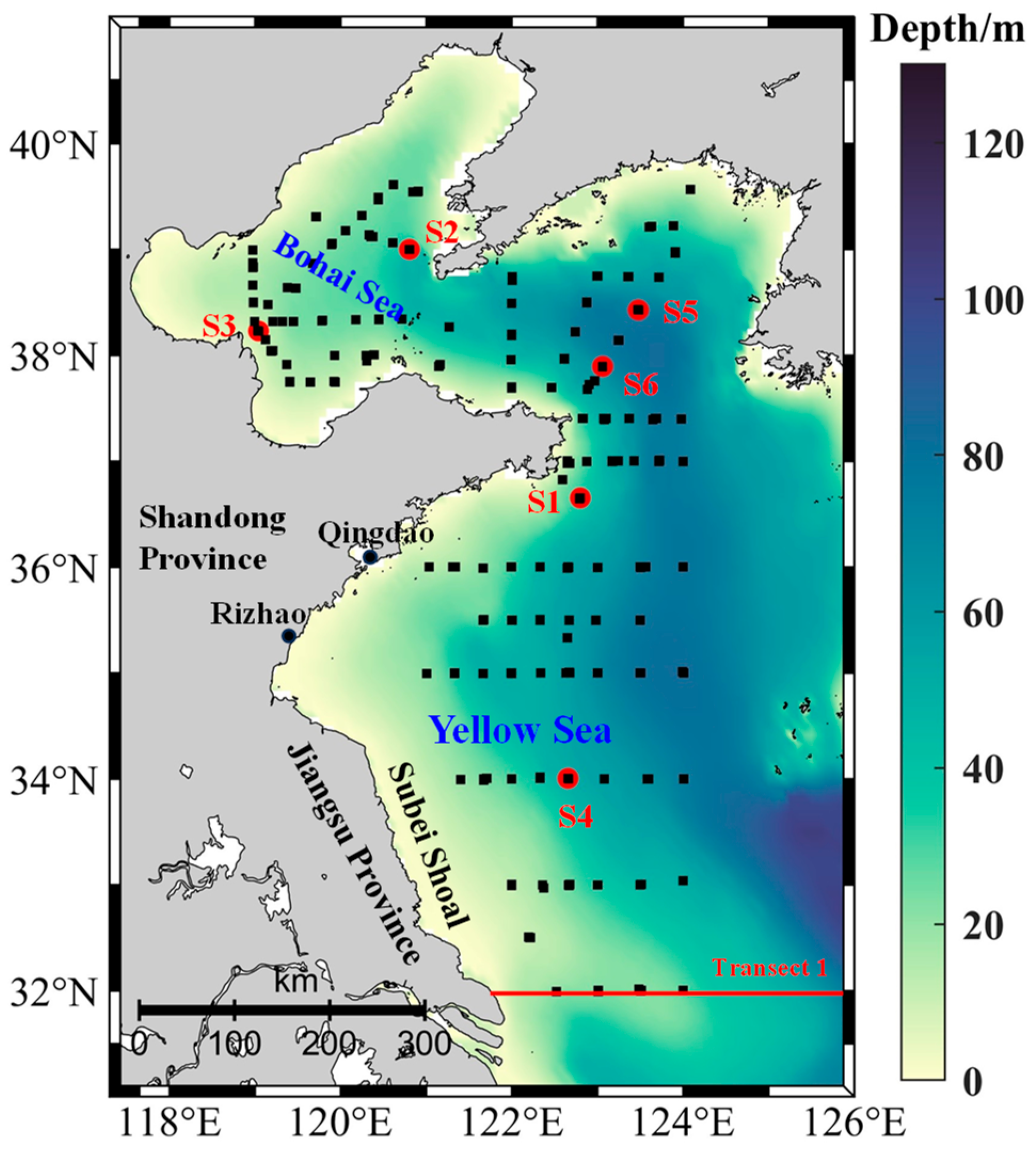
2.2. In Situ Measurements

In situ measurements in the BSYS were collected during three cruises aboard the R/V Dongfanghong 2 in winter (December 2016), spring (April 2018), and summer (July 2018). The locations of the sample stations are shown in Figure 1.
In situ TSM concentrations at various water layers at each station were obtained through laboratory measurements. During the survey, TSM concentrations were measured in the surface, middle, and bottom water layers at each station. The water depths for sample collection were determined based on the water depth at each station. The steps for measuring TSM concentrations were as follows: Before the cruise, 47 mm Whatman GF/F glass fiber filters were pre-weighed to an accuracy of 0.01 mg (marked as W1). During the cruise, seawater samples were collected from different layers (surface, middle, and bottom) at each station. A specified volume (0.5–2 L) of each water sample (marked as V) was then filtered under a vacuum pressure of 0.01 MPa. After filtration, the filters were rinsed three times with Milli-Q water and subsequently stored at −20 °C. In the laboratory, the filters were dried at 105 °C for 4 h and reweighed to obtain their post-weight (marked as W2). The TSM concentrations were calculated by dividing the difference between the post-weight (W2) and the pre-weight (W1) by the filtration volume (V), according to Equation (1).
TSM = W 2 W 1 / V
It is important to note that several potential sources of error may affect TSM measurements. (1) Errors in measuring the volume of filtered water samples. To minimize this error, we employed a graduated cylinder with an accuracy of 1 mL. (2) Weighing errors associated with the electronic balance used for the filters. To ensure accuracy, each filter was weighed repeatedly until the difference between the last two measurements was within 0.02 mg. (3) Residual salt from seawater samples can affect the weight of the dried filters, thus influencing TSM concentration. To remove potential residual salt, we rinsed the filters three times with 50 mL of Milli-Q water after filtration.
At each station, a suite of instruments was deployed to measure various parameters: a Seabird SBE911P conductivity–temperature–depth (CTD) profiler (Seabird Scientific, Bellevue, WA, USA) for water temperature, a Sequoia Scientific LISST-100X (Sequoia Scientific, Inc., Bellevue, WA, USA) for particle size (DA) and number concentration (N0), an ECO Triplet (Wetlabs, Philomath, OR, USA) for turbidity (Turb), a WET Labs AC-S (Wetlabs, Philomath, OR, USA) for absorption coefficient (a(λ)) and attenuation coefficient (c(λ)), and a HOBI Labs Hydroscat-6 (HOBI Labs, Inc., Redmond, WA, USA) for backscattering coefficient (bb(λ)). For detailed information on the measurements, including DA and N0, please refer to Wang et al. [19]. Additionally, particle backscatter coefficient bbp(λ) was calculated by subtracting the backscattering coefficient of water (bb,w(λ)) from bb(λ) [43], as defined in Equation (2).
b bp λ = b b λ     b b , w λ

2.3. Optical Satellite and Environmental Data

The objective of this study was to achieve remote monitoring of the vertical distribution of TSM concentration using satellite observations from the Moderate Resolution Imaging Spectroradiometer (MODIS) onboard the Aqua satellite. MODIS ocean color data have been extensively utilized in marine environmental monitoring, including water color parameter inversion and water quality assessment. In the visible region, the MODIS sensor is equipped with ten wavebands featuring central wavelengths of 412, 443, 469, 488, 531, 547, 555, 645, 667, and 678 nm.
In this study, standard monthly Aqua-MODIS remote sensing reflectance (Rrs) and sea surface temperature (SST) Level 3 products, with a spatial resolution of 4 km, were obtained from the NASA Ocean Color website (http://oceancolor.gsfc.nasa.gov/; accessed on 10 August 2023). These products span the period from January 2003 to December 2021. It should be noted that the TSM vertical distribution estimation model proposed in this study (see Section 2.4.3) required the surface TSM concentration (TSMsurf). However, Aqua-MODIS does not provide TSMsurf as a standard product. Thus, satellite TSMsurf data were derived from the MODIS Rrs product using the YOC algorithm proposed by Siswanto et al. [29], as described in Equation (3).
TSM surf = 10 0 . 649 + 25 . 623 × X 1 0 . 646 × X 2
where X1 = Rrs(555) + Rrs(667), X2 = Rrs(488)/Rrs(555).
Additionally, to differentiate the vertical types of TSM distribution, this study investigated the relationship between TSM vertical profile types and various marine environmental factors. Specifically, we focused on three key environmental factors: sea surface temperature (SST), sea surface wind, and water depth. SST data in the BSYS were sourced from Aqua-MODIS SST products. Sea surface wind data at 10 m above sea level were obtained from the monthly CCMP wind vector analysis product (CCMP V2.0) with a spatial resolution of 0.25° × 0.25°, available from Remote Sensing Systems (https://www.remss.com/measurements/ccmp/; accessed on 15 August 2023). The water depth dataset (bathymetry) was sourced from the ETOPO global Relief Model (version 2022) with a 15 arc-second resolution (https://www.ncei.noaa.gov/products/etopo-global-relief-model/; accessed on 22 August 2023). All datasets used in this study were resampled to a spatial resolution of 4 km for consistency.

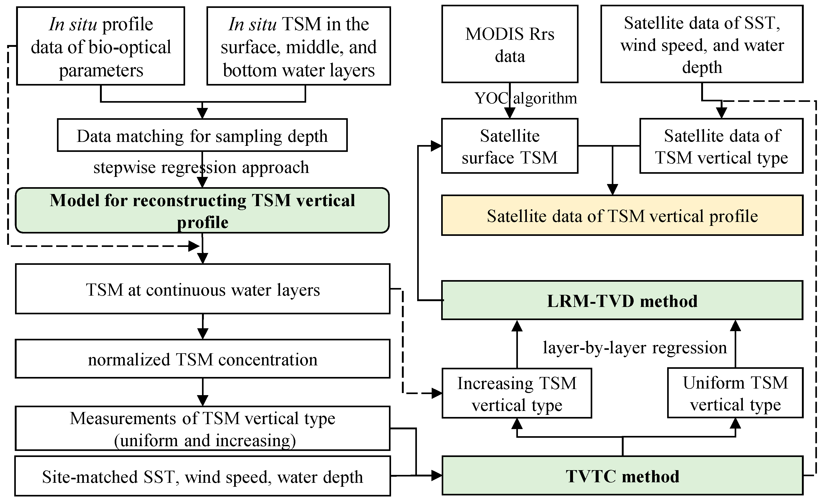
2.4. Estimation Method for TSM Vertical Distribution

The objective of this study was to estimate the vertical profile of TSM from satellite observations. As illustrated in Figure 2, the workflow for the remote sensing estimation of TSM vertical profiles comprises the following parts: (1) reconstructing in situ TSM vertical profiles from field measurements of various bio-optical parameters (see Section 2.4.1); (2) classifying TSM vertical types using the proposed TVTC method (see Section 2.4.2); (3) estimating TSM concentrations at different water layers employing LRM-TVD method (see Section 2.4.3); and (4) satellite estimation of TSM vertical profiles using the TVTC and LRM-TVD methods based on MODIS Rrs and environmental data (see Section 2.4.4).

2.4.1. Model for Reconstructing In Situ TSM Vertical Profile Data

The dataset of in situ TSM vertical profiles is crucial for studying and analyzing the various vertical types of TSM distribution in the BSYS. However, due to the extensive measurement efforts required, obtaining comprehensive TSM vertical profile in practical operations is challenging. To address this problem, an empirical algorithm (see Equation (4)) was proposed to reconstruct in situ TSM vertical profile from the measured profile data of multiple optical parameters, including particle number concentration, turbidity, particle backscattering coefficient, and attenuation coefficient. Given the linear correlation between TSM concentrations and optical parameters in a logarithmic coordinate system, Equation (4) adopted a log-linear form. A stepwise regression approach was used to select the optimal variables for this reconstruction algorithm (see Section 3.1 below). Once the necessary optical parameter data are available, the in situ TSM vertical profile data can be reconstructed using Equation (4).
log 10 ( TSM ) = a 0 + a 1 × log 10 ( x 1 ) + a 2 × log 10 ( x 2 ) + + a n × log 10 ( x n )
where x1, x2, … xn are the bio-optical parameters, and a0, a1, … an are the fitting coefficients.

2.4.2. Classification Method of TSM Vertical Profile Types

To estimate the TSM vertical distribution, it is crucial to identify the TSM vertical type first. The types of TSM vertical profiles in the BSYS were investigated based on the in situ reconstructed TSM profile data using Equation (4). To better illustrate the vertical characteristics of TSM concentration at different water layers, dimensionless processing was applied to the in situ reconstructed TSM vertical profile. This process involved normalizing the actual water layers to a dimensionless scale ranging from 0 to 1, enabling direct comparison between different water layers. Consequently, the relative depth (hr) and the corresponding normalized TSM concentration (NTSM (hr)) were calculated as follows:
h r z = 1 z H NTSM h r = TSM h r TS M surf
where hr (z) denotes the relative water depth at the actual water layer z (m), and H is the water depth of the observation point (m). For example, the relative depths at the surface, middle, and bottom layers are 1, 0.5, and 0, respectively. By visually interpreting the reconstructed TSM vertical distribution characteristics from 223 samples in the BSYS, we identified two broad categories of TSM vertical types: uniform and increasing, as shown in Figure 3. It is important to emphasize that we employed visual interpretation to ensure the accuracy of the classification. However, when the dataset is large, the optimal approach is to quantitatively characterize the vertical distribution of each sample using an appropriate mathematical model and then automatically classify the distribution types based on the parameters of the quantitative model. This would not only enhance the efficiency of the classification process but may also yield a wider variety of TSM vertical distribution types. Further in-depth research on this issue will be necessary in future work.
The vertical distribution of TSM concentration is influenced by a combination of environmental factors, including sea surface temperature, topography, and wind speed [11,12]. In this study, field measurements of TSM vertical types were classified based on the normalized TSM vertical profile, with values of 0 assigned to uniform types and 1 to increasing types. To develop the classification method for TSM vertical types, referred to as the TVTC method, field-measured TSM vertical types and site-matched environmental parameter data were input into the Chi-squared Automatic Interaction Detector (CHAID) approach. The CHAID is a statistical modeling technique that utilizes the Chi-squared test and a tree structure to address classification problems [44]. CHAID identifies significant associations and interactions between variables by detecting feature interactions and constructing a decision tree. The fundamental principle of the CHAID approach is to optimally partition the sample according to the relationships between input features and target variables, automatically determining the grouping of multivariate categories based on the significance of the chi-squared test. This approach facilitates the rapid and efficient identification of key influencing factors [44,45].
Ultimately, three environmental parameters—SST, water depth, and wind speed—were identified as the optimal influencing factors for TSM vertical types. These parameters served as input variables for the CHAID approach to develop the TVTC method in our study (refer to Figure 7 below for detailed information).

2.4.3. Estimating TSM Concentrations at Different Water Layers

After identifying the TSM vertical type using the TVTC method, the TSM concentrations at continuous water layers (i.e., the TSM vertical profile) were estimated based on whether the distribution was of the uniform or increasing type. For the uniform TSM vertical type, the TSM concentrations at different water layers were assumed to be equal to the TSMsurf concentration. For the increasing TSM vertical type, a layer-by-layer regression method for estimating the TSM vertical distribution (hereafter referred to as the LRM-TVD method) was employed. This method is built upon previous studies on TSM vertical distribution in lake waters [42].
The main steps in the development of the LRM-TVD method were as follows: firstly, based on the actual water depth z for sample stations, the relative water depth hr was calculated and divided into to 11 layers using Equation (5). The hr ranged from 1 (representing the surface layer) to 0 (representing the bottom layer) with an interval of −0.1. Then, a quantitative relationship was established between the TSM concentrations at ±0.1 hr. Specifically, the relationship between TSM (hr = 1) and TSM (hr = 0.9) was established, and this process was continued to establish relationships between subsequent pairs of relative water depths (see Figure 8 below). When applying the LRM-TVD method at an observation point, the hr with 11 layers was derived from the actual water depth. The established LRM-TVD method was then used to estimate TSM concentrations at different hr layers. The relative water depth hr was converted to actual water depths z. In this way, the TSM vertical distribution can be estimated for the increasing type.

2.4.4. Satellite Estimation of TSM Vertical Profile

Based on satellite products of SST, wind speed, and water depth, the TSM vertical types were derived using the proposed TVTC method. Satellite-derived TSMsurf data were then obtained from MODIS Rrs data using the YOC algorithm. By integrating satellite-derived TSM vertical types, the vertical distribution of TSM was estimated using LRM-TVD method.

2.5. Accuracy Assessment

In this study, a confusion matrix was employed to assess the performance of the TVTC method in classifying TSM vertical types. The confusion matrix is widely used to evaluate the accuracy of classification methods [46]. Statistical indicators derived from the confusion matrix were used to quantitatively evaluate the classification accuracy [47], including precision, recall, and overall accuracy. Meanwhile, to assess the agreement between the measured and estimated TSM profile data, the coefficient of determination (R2), mean absolute percentage error (MAPE), and root mean squared error (RMSE) were employed as follows:
MAPE = 1 n i = 1 n x i y i x i × 100 %
RMSE = 1 n i = 1 n x i y i 2
where xi and yi denote the measured data and model-estimated data, respectively.

3. Results

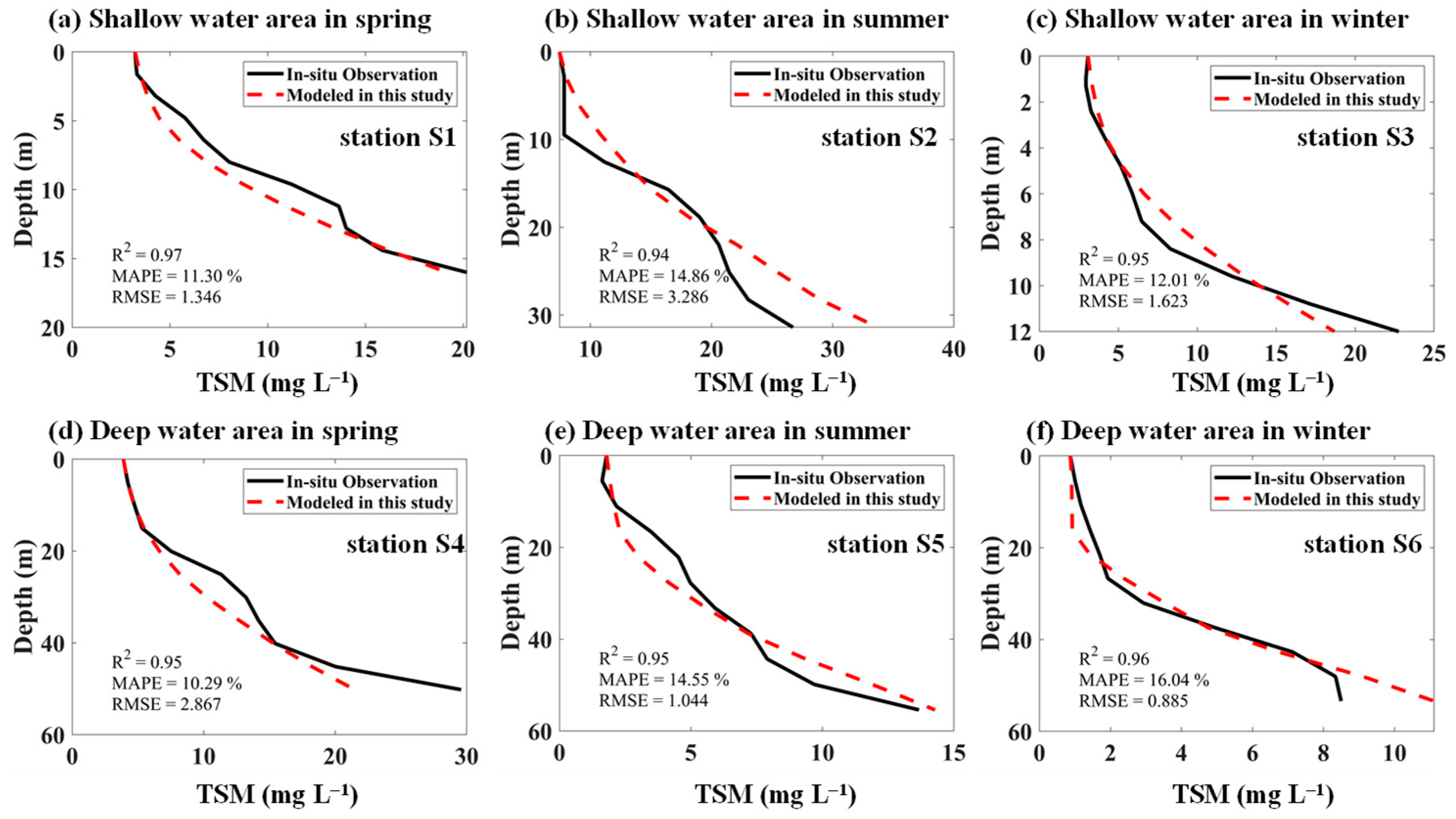
3.1. Analysis of the TSM Vertical Distribution Based on In Situ Measurements in the BSYS

To obtain in situ TSM profile data, the correlations between TSM concentration and particle size distribution and related optical parameters were examined to develop a multi-parameter model for reconstructing the TSM vertical profile, as defined in Equation (4). Based on the field measurement at the surface, middle, and bottom water layers, the R2 (R2 ≥ 0.72; see Figure 4) indicated a strong correlation between the TSM concentration and bio-optical parameters, including the particle size (DA), particle number concentration (N0), bbp(442), bbp(700), bbp(488), bbp(550), bbp(620), bbp(852), and c(670). DA and N0 exhibited strong correlations with the measured TSM concentration, with R2 values of 0.72 and 0.73, respectively. Turbidity showed a higher correlation with the TSM concentrations (R2 = 0.85). The optical parameter bbp(λ) showed strong correlations with TSM concentrations across wavelengths of 442, 488, 550, 620, 700, and 852 nm, all with R2 values greater than 0.86. The correlation improved with increasing wavelength, indicating higher concentrations of inorganic suspended matter in the BSYS. Similarly, c(670) also showed a strong correlation with TSM concentrations (R2 = 0.85), suggesting that the attenuation effect of higher TSM concentrations on water bodies is significant. The strong correlations and seasonal stability between TSM concentrations and various bio-optical parameters provide a foundation for developing a multi-parameter model to reconstruct the TSM vertical distribution. It is important to note that these robust correlations were observed through local field measurements. While the data-driven correlations may be applicable to other marine regions, further data validation is necessary.
Here, to select the optimal variables as inputs for the TSM profile reconstruction model, a stepwise regression approach was employed in this study. The in situ measured samples were randomly divided into training (70%) and testing (30%) datasets in a 7:3 ratio to ensure the independence of the training and testing datasets. Through stepwise regression, DA, N0, Turb, bbp(442), bbp(488), bbp(550), bbp(620), bbp(700), bbp(852), and c(670) were ultimately selected as inputs. Equation (4) was fitted to 156 pairs of the measured TSM concentrations and the above parameters to develop the TSM profile reconstruction model. The established parameters and their coefficient are shown in Table 1. Figure 5 displays the comparison between the estimated and measured TSM concentrations for the training and testing datasets. It can be seen that the estimated TSM concentrations agreed well with the measured TSM concentrations, with R2 = 0.9, RMSE < 9.5, and MAPE < 26.5%. All samples were close to the 1:1 line. The results suggest that the proposed TSM profile reconstruction model demonstrated strong performance and can accurately obtain the TSM vertical profile.
For the 223 samples in the BSYS, the vertical distribution of TSM concentrations was obtained using the TSM reconstruction model with the coefficients provided in Table 1. The NSTM (hr) profile data were then calculated following Equation (5), and their TSM vertical types were classified based on the rate of increase in the NTSM profile. Statistical analysis showed that 42.6% (N = 95) of all stations exhibited the uniform type of TSM vertical distribution, while 57.4% (N = 128) of all stations showed the increasing type. Additionally, we analyzed the seasonal variations of TSM vertical types (Figure 6). In the BSYS, both the uniform and increasing types of TSM vertical distribution were observed in spring, summer, and winter, with their proportions varying by season. In spring, the proportions of uniform (51.7%) and increasing types (48.3%) were nearly equal. In summer, the increasing type was overwhelmingly dominant, constituting approximately 93.7%. In winter, the uniform type (59.8%) was predominant, slightly higher than the increasing type (40.2%). Furthermore, the TSM vertical distribution types exhibited regional differences, as shown in Figure 6. In relatively shallow areas such as the BS and North Yellow Sea (NYS), the uniform type predominated in spring and winter. In the South Yellow Sea (SYS), the increasing type was more prevalent in spring and winter, particularly in relatively deeper areas.

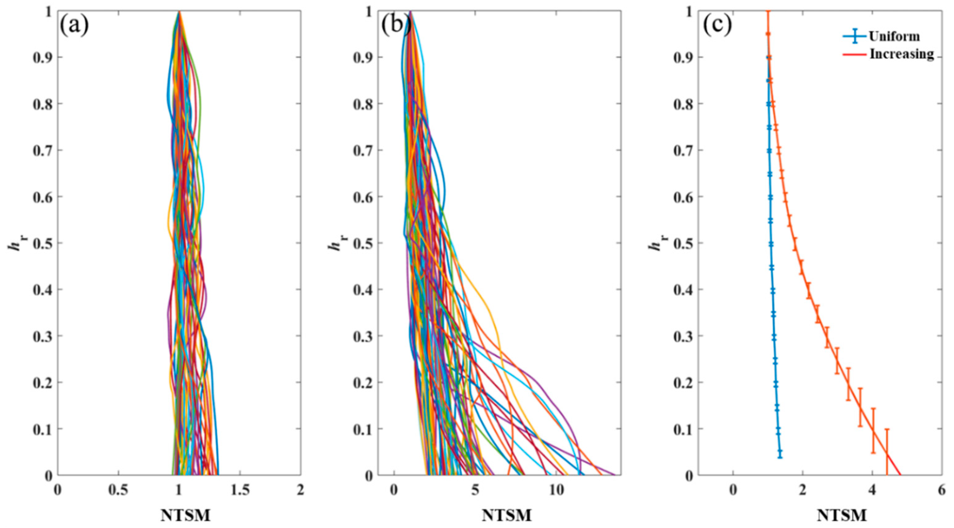
3.2. Identification of TSM Vertical Profile Types

Using in situ TSM vertical type and synchronous environmental factors (including SST, water depth, and wind speed), we employed the CHAID approach to develop the TVTC method. The purpose of the TVTC method was to discriminate the TSM vertical type using readily obtainable environmental variable data. To assess the performance of the proposed TVTC method, the field-measured dataset was randomly divided into training and testing datasets in a 7:3 ratio, ensuring the independence of the training and testing datasets. Figure 7 shows the specific classification criteria of the TVTC method for discriminating the TSM vertical type in the BSYS.
Figure 7. Classification criteria of the TVTC method in the BSYS.
Remotesensing 16 03736 g007
Table 2 presents the accuracy evaluation statistics for the training and testing datasets. In the training set, the classification model achieved 85.0% precision for the uniform type and 84.3% for the increasing type, resulting in an overall accuracy of 84.7%. Similarly, in the testing set, the precision of the classification model was 84.6% for the uniform type and 82.9% for the increasing type, yielding an overall accuracy of 83.8%. These results indicate that the TCTV method proposed in this study can effectively classify the vertical types of TSM concentration in the BSYS.

3.3. Development of the LRM-TVD Method

Following Section 2.4.3, the layer-by-layer regression approach was applied to the in situ reconstructed TSM vertical profile using a linear least-squares fitting procedure to develop the LRM-TVD method, as illustrated in Figure 8. The strong linear relationships between TSM concentrations in adjacent relative water layers were observed, with R2 values ranging from 0.91 to 0.98 and MAPE values between 18.31% and 35.91%. These results indicate that the LRM-TVD method provided a reliable framework for estimating the TSM vertical profile.
Figure 8. Correlation between TSM concentrations at adjacent relative water layers.
Remotesensing 16 03736 g008
In this study, the LRM-TVD method was applied to field samples to estimate the TSM vertical distribution based on surface TSM concentrations and the water depth. Examples of the estimated TSM vertical distribution obtained using the LRM-TVD method across various seasons and water depths are presented in Figure 9. It can be observed that the estimated TSM vertical distribution curves closely align with the measured TSM vertical curves. The correlation between the model-estimated and measured TSM values was high, with R2 ≥ 0.95 and MAPE ≤ 16%. The mean MAPE for all samples was 38.03%. Furthermore, the LRM-TVD method for estimating TSM vertical profile demonstrated seasonal stability across spring, summer, and winter and performed effectively in both shallow and deep waters (Figure 9).
Figure 9. Comparison between the model-derived TSM vertical profile and in situ reconstructed TSM vertical profile for the example stations, with their locations shown in Figure 1.
Remotesensing 16 03736 g009

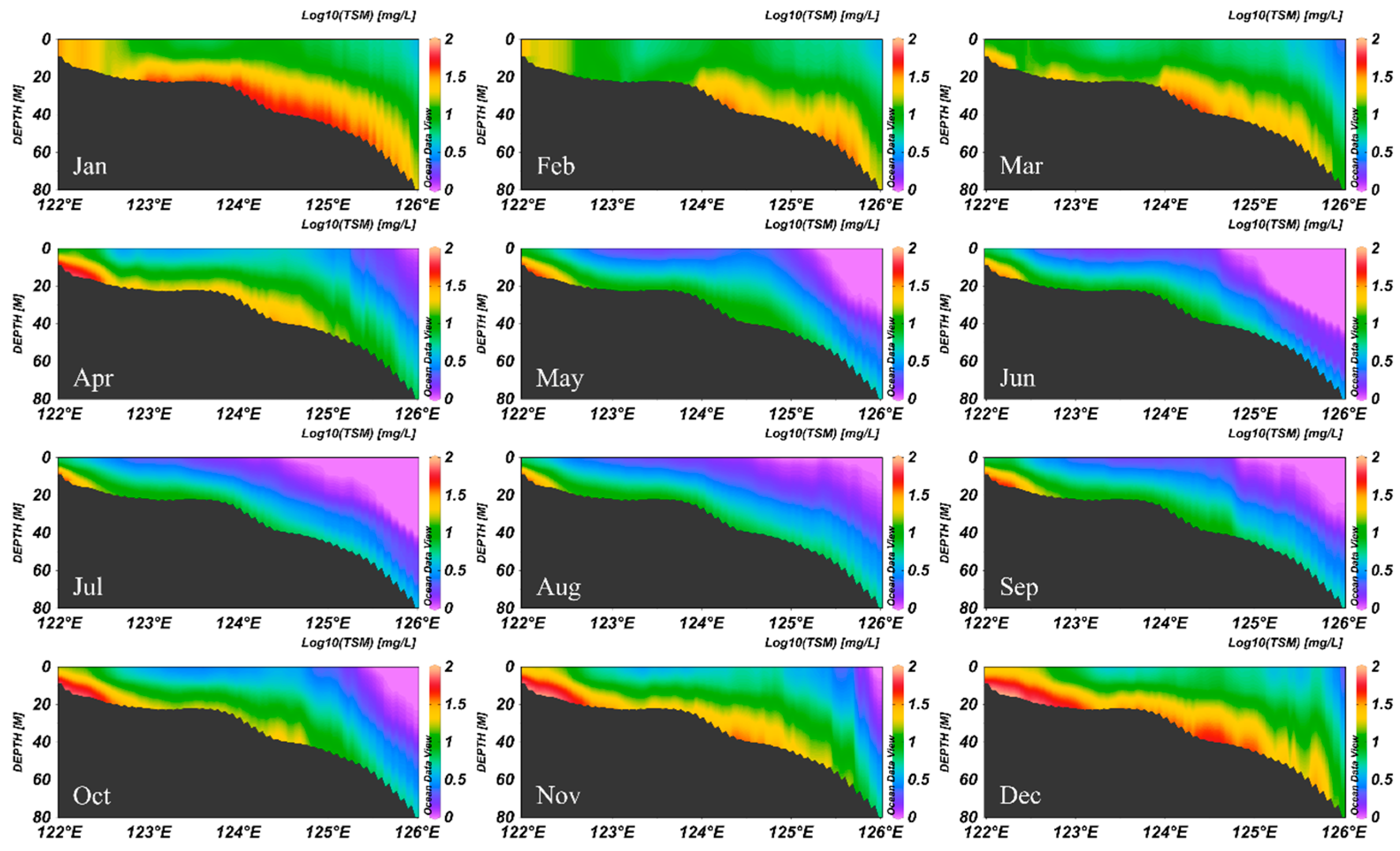
3.4. Estimating TSM Vertical Distribution for Satellite Application in the BSYS

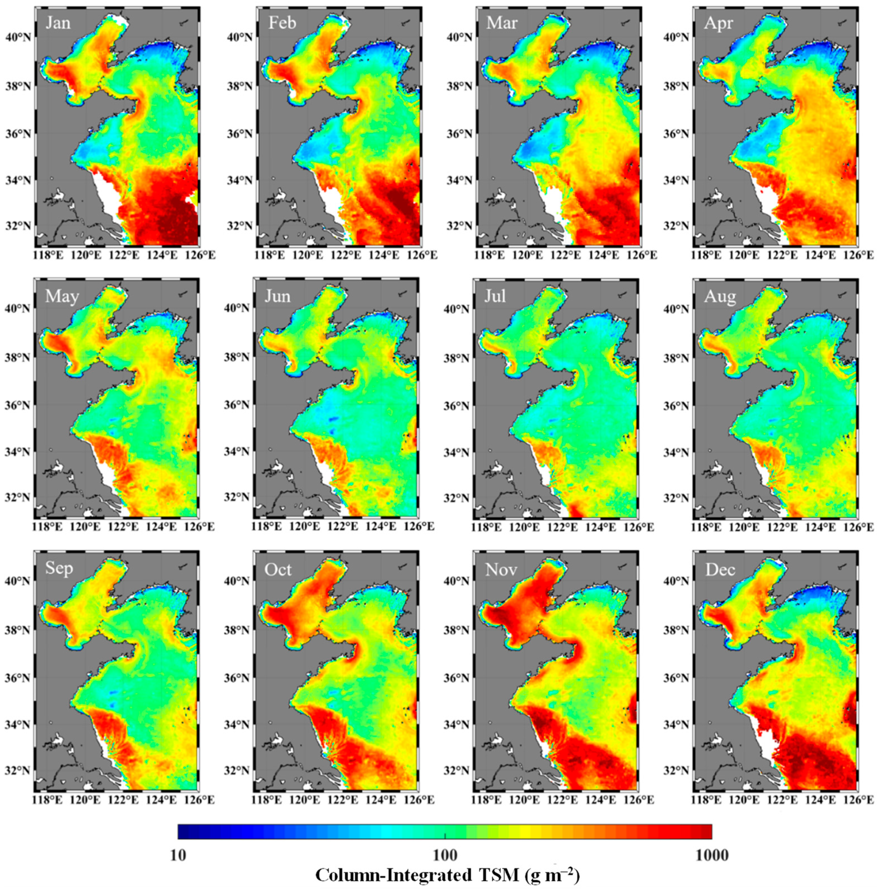
3.4.1. Spatiotemporal Variation of TSM Vertical Type

Based on monthly satellite data of SST, wind speed, and water depth, monthly satellite products of TSM vertical types in the BSYS were generated using the proposed TVTC method. Subsequently, the proportions of uniform and increasing TSM vertical types were calculated from January to December to effectively present their variability, as shown in Figure 10. During the winter months (December, January, and February), the Bohai Sea region predominantly exhibited a uniform TSM vertical type. However, in January, a low proportion of the increasing TSM vertical type was observed in the Bohai Strait and the central Bohai Sea. This observation aligns with the lower proportion (6.4%) of the increasing TSM type in winter (see Figure 6). In early and mid-spring (March and April), the TSM concentrations in the BS primarily displayed a uniform type. By late spring (May), with rising temperatures, the TSM vertical distribution type shifted to the increasing type, which persisted through summer (June, July, and August) and autumn (September, October, and November). In the northern area of the Yellow Sea (NYS), the spatial pattern of TSM vertical types during winter and early spring resembled that of the Bohai Sea, with the uniform type being predominant. This was consistent with field-measured results in Figure 6, which showed that the uniform type accounted for approximately 92.9% in the northern area of the Yellow Sea during winter. Starting in April, the TSM vertical distribution type gradually transitioned to the increasing type, which persisted until November. In contrast, the southern area of the Yellow Sea, located at a lower latitude and connected to the open sea, has deeper waters and maintains higher SST throughout the year. The southern area of the Yellow Sea exhibited the highest proportion of the increasing type throughout most months of the year. Nevertheless, during winter (December, January, and February) and early spring (March), the uniform type of TSM vertical distribution was predominant in the nearshore waters.
Overall, the TSM vertical types exhibited notable seasonal and regional variations. The patterns of TSM vertical types derived using the TVTC method closely matched the statistical results from field investigations, demonstrating that the TVTC method can effectively classify TSM vertical types from satellite observations.

3.4.2. Estimation of TSM Vertical Distribution from MODIS Data

To obtain satellite products of the TSM vertical distribution, we first obtained satellite TSMsurf data from the monthly MODIS Rrs data using the YOC algorithm, as described in Equation (3). Based on site-matched MODIS Rrs and field-measured TSM concentrations, a high degree of consistency was observed between the satellite YOC-estimated TSM and field-measured TSM concentrations, with R2 = 0.9 and MAPE = 33.8%. This indicates that the YOC algorithm performs well for estimating TSMsurf in the Bohai Sea and Yellow Sea. Then, we applied the LRM-TVD method to generate monthly satellite TSM vertical distribution products for the BSYS from 2003 to 2021, along with satellite TSM vertical-type products. Figure 11 illustrates the monthly TSM vertical distribution for a representative transect (32°N, 122°–126°E) over 12 months. The TSM concentrations in the horizontal direction displayed a spatial pattern with high concentrations nearshore and low concentrations offshore. Vertically, the cross-sectional area showed an increasing spatial distribution throughout the year, with low surface TSM concentrations and high bottom TSM concentrations. Additionally, the vertical distribution of TSM concentrations exhibited significant seasonal variation, with higher levels in autumn (September, October, and November) and winter (December, January, and February) and lower levels from March to August.
Figure 11. Monthly vertical distribution of TSM concentrations at the representative transect (32°N, 122°–126°E), with its location indicated in Transect 1 in Figure 1, covering the period from January to December. The numbers on the color bar represent TSM concentration in logarithmic coordinates.
Remotesensing 16 03736 g011
Furthermore, the monthly column-integrated TSM concentrations in the BSYS were generated by integrating the TSM vertical profile distribution across the entire water column. This integration reflects the comprehensive nature of the TSM vertical distribution, as it is influenced not only by the TSM profile concentrations but also by the water depth. Here, we analyzed the spatial and temporal variations of the column-integrated TSM concentrations in the BSYS, as shown in Figure 12. In general, the column-integrated TSM concentrations in the BSYS exhibited significant spatiotemporal differences. Temporally, the column-integrated TSM concentrations were higher in early spring (March and April), late autumn (October and November), and winter (December, January, and February), with particularly high levels during the winter months. From May to September, the concentrations were lower. Spatially, the column-integrated TSM concentrations remained high in the shallow Bohai Sea region, where the water depth is less than 30 m, resulting in consistently high values throughout the year. In contrast, the central region of the South Yellow Sea, with water depths of 60–80 m, exhibited lower concentrations. Additionally, relatively high levels of column-integrated TSM concentrations were observed in the shallow waters of Northern Jiangsu and the Yangtze River mouth and its adjacent areas.

4. Discussion

4.1. Comparison with Theoretical Model

Theoretically, the vertical distributions of TSM can be described using the diffusion theory model [48,49]. According to this classical theory, the normalized TSM, defined as the ratio of TSM concentration at any depth to that at the surface layer, exhibits an exponential relationship with the natural constant as the base. This relationship can be expressed as follows:
NTSM h r = TSM h r TSM surf = e a b × h r
where TSM (hr) and TSMsurf denote the TSM concentrations at the relative depth hr and surface layers, respectively; a and b represent the model parameters. We validated the performance of the diffusion theory model using our field-measured dataset, finding that it accurately represents the vertical distribution of TSM in the Bohai and Yellow Seas. The R2 values for all samples exceed 0.6, with more than 90% of the samples having R2 values above 0.8. Additionally, the MAPE values for all samples are below 50%, and for more than 80% of the samples, the MAPE value are within 30%.
Although the diffusion theory model showed good performance in simulating the vertical distribution of TSM concentration, it has notable limitations when applied to satellite remote sensing data. We observed significant spatial and seasonal variations in the model parameters a and b, which exhibited poor correlation with key marine environmental parameters, including water depth, wind speed, sea surface temperature (SST), sea surface salinity (SSS), and TSM at the surface layer (Table 3). For the diffusion theory model to accurately estimate the TSM vertical distribution using satellite observations, parameters a and b must be known or estimated from numerical or satellite-derived environmental data. However, the significant variations and weak correlations of these parameters with environmental factors hinder the model’s practical application. A potential strategy to address this limitation is to create a lookup table for parameters a and b based on a larger in situ dataset. Although we collected 223 in situ samples across the BSYS over three seasons, this dataset remains insufficient to develop a comprehensive lookup table, thereby restricting the remote sensing application of the diffusion theory model at this stage.
Compared with the diffusion theory model, the estimation model established in this study, while having relatively lower fitting accuracy, still demonstrated acceptable performance, with a mean MAPE value of 38.03% for all samples. More importantly, by combining the estimation model (i.e., the LRM-TVD model) with the classification method of TSM vertical profile types developed in this study, we successfully estimated the vertical distributions of TSM from satellite remote sensing data and obtained their reasonable spatial–temporal variations (Figure 11).

4.2. Rationality and Applicability of the Estimation Approach

The vertical distribution of TSM often undergoes significant variations in response to changes in hydrographic environmental factors in coastal regions [12,15,16,50]. Among these factors, the water temperature is fundamental in determining distinct vertical distribution patterns of TSM. Specifically, the sea surface temperature (SST) serves as a proxy for energy input into the water column, with higher SST values indicating greater energy influx and stronger water stratification [51,52,53]. Moreover, the water depth influences TSM vertical profiles, as it governs the penetration of energy throughout the water column [54,55]. Deeper waters facilitate more effective energy transmission and mixing [56]. Additionally, the vertical distribution patterns of TSM are also modulated by the sea surface wind speed by influencing the degree of water mixing and sediment resuspension [57]. Overall, the interplay of these hydrographic environmental factors orchestrates the intricate vertical distribution patterns of TSM concentrations across different seasons through processes of water stratification, mixing, and sediment resuspension.
For instance, during summer, the vertical distribution of TSM concentrations clearly demonstrates an increasing gradient. This phenomenon is attributable to the combined effects of elevated temperatures, stable water stratification, and diminished wind speeds, which impede effective seawater mixing [58,59]. Consequently, TSM concentrations ascend throughout the water column during the summer season. In contrast, the vertical distribution patterns of TSM exhibit regional disparities during the spring and winter seasons, driven by variations in water temperature and wind conditions. During winter, as temperatures drop, the surface water density increases. Additionally, winter wind fields tend to be more vigorous than those in summer, fostering enhanced sediment resuspension in shallow water areas and promoting robust vertical mixing [60,61]. As a result, the TSM vertical profile in shallow waters tends to exhibit a relatively uniform distribution from the surface to the seafloor, manifesting a dominant pattern of uniform distribution. However, in deep water regions, despite the intensified winter wind fields, the mixing remains insufficient to thoroughly homogenize the water column [62,63]. This results in uneven mixing and a marginal predominance of an incremental-type distribution.
The classification method for the vertical distribution types of TSM proposed in this study is based on the relationship between the vertical distribution patterns of TSM and marine environmental factors, ensuring the rationality of our approach. Through the analysis of over two hundred field-observed samples from the Bohai and Yellow Seas across different seasons, we established robust principles for classifying the vertical distribution patterns of TSM using the water depth, SST, and wind speed—all of which can be derived from satellite products. This foundation allows for the effective application of our classification method to determine the vertical distribution types of TSM from satellite observations.
To estimate the vertical distribution of TSM, the first step involves classifying the vertical type, followed by the essential task of estimating TSM at different layers throughout the entire water column. As discussed in Section 4.1, applying the theoretical diffusion theory model to satellite remote sensing data is infeasible. Therefore, this study employs a layer-by-layer regression method (i.e., the LRM-TVD method) to estimate the vertical distribution of TSM. Although the layer-by-layer regression method is empirical and lacks the theoretical foundation of the diffusion theory model, it demonstrates good estimation accuracy. Previous studies, such as Lei et al. [27], have shown that this method performs well in lake environments. More importantly, the method utilized in this study is applicable to satellite remote sensing data, enhancing the model’s practicality.

4.3. Implications and Suggestions for Future Work

The vertical distribution of TSM is crucial for studying marine environments and biogeochemical processes [5,8,9]. Traditional field observations are limited in spatial and temporal coverage, making the exploration of remote-sensing technology essential for acquiring comprehensive information on the vertical distribution of TSM over broad spatial and temporal coverages. In this study, we analyzed the vertical distribution characteristics of TSM in the Bohai and Yellow Seas, explored their relationships with environmental variables, and developed the TVTC and LRM-TVD methods. Our findings demonstrate the feasibility of estimating TSM vertical profiles from satellite observations. These satellite-based estimations enhance the understanding of the spatial and temporal variations in TSM vertical distribution in the Bohai and Yellow Seas. Furthermore, they provide valuable insights and support for studies on material transport, sedimentation processes, and geomorphological evolution.
Despite the promising results obtained in this study, several limitations and suggestions require further investigation in future research. We utilized an optical reconstruction model to derive in situ vertical distributions of TSM from optical measurements, including the backscattering coefficient, attenuation coefficient, and water turbidity. By leveraging the strong relationships between these optical parameters and TSM, the model provides a valuable tool for accurately inferring nearly continuous vertical profiles of TSM in water columns. This approach significantly improves the vertical resolution of TSM profiles and measurement efficiency, overcoming the limitations of traditional TSM measurements, which rely on the gravity method and can only obtain TSM at several dispersed depths. However, this approach is based on the crucial assumption that optical properties are indicative of TSM and can be used to reconstruct the vertical distribution. Although the strong relationships between TSM and optical properties have been widely documented by the marine optics community in various waters [12,14,25,26], these relationships can vary across different waters [19,23]. Consequently, at this stage, we can only confirm that the reconstruction model proposed in this study is suitable for the Bohai and Yellow Seas. Our reconstruction approach provides a useful reference for developing region-specific reconstruction models for other marine waters in future research.
To estimate TSM at different depths, this study employed a layer-to-layer regression approach known as the LRM-TVD model. Although the model generally showed good performance, we found that the model parameters differed from those used by Lei et al. [27], who applied the same approach to estimate TSM vertical profiles in Lake Hongze. This indicates that the LRM-TVD model relies on region-specific empirical relationships between TSM at adjacent layers. Therefore, understanding the complex interactions and dynamics between layers in various waters is essential for accurately estimating the vertical distribution of TSM. Further research should focus on elucidating these interlayer relationships and exploring additional parameters that can enhance the determination of TSM profiles.
Meanwhile, this study classified the vertical distribution of TSM into two types: uniform and increasing. However, this classification may be somewhat simplistic. By subdividing vertical distribution types further, we could achieve a more detailed representation of distribution type changes from coastal to offshore regions. We attempted to categorize the types into more specific categories; however, we found that this increased complexity made it challenging to estimate TSM vertical concentrations, likely due to our limited dataset of 223 samples. Therefore, we plan to collect additional in situ data in the future to facilitate a more refined classification of vertical distribution types. Once we have sufficient sample data for each type, it may be feasible to apply appropriate mathematical models to establish accurate TSM vertical concentration estimation models for various distribution types.
In addition, as discussed in Section 4.1, we found that the diffusion theory model provides better estimation accuracy for the vertical distribution of TSM at each site. However, its application in satellite remote sensing is limited due to significant spatial and seasonal variations in model parameters and the inability to infer these parameters using environmental variables. If sufficient, spatially comprehensive, and seasonally comprehensive in situ measurement data were available, a lookup table for the diffusion theory model parameters could be established. This would be another method for achieving vertical distribution estimation of TSM via satellite remote sensing. However, the current lack of sufficient in situ measurement data makes it difficult to establish a reliable lookup table. Therefore, we suggest that future research focus on acquiring more in situ measurement samples to establish such a lookup table for the theoretical model parameters. This would ultimately enable the use of the theoretical model for the vertical distribution estimation of TSM via satellite remote sensing.
Overall, the optical reconstruction model, classification method, and LRM-TVD model employed in this study offer a new perspective and a useful approach to understanding the vertical distribution of TSM in marine waters. Despite the above discussed limitations, these methods provide valuable insights into the vertical distribution characteristics of TSM from satellite observations. Future research should aim to refine and improve these approaches to overcome the identified limitations and expand their applicability to a broader range of water bodies and environmental conditions.

5. Conclusions

Estimating the vertical distribution of TSM concentrations plays a critical role in studying marine environment and biogeochemical processes. Based on extensive in situ measurements acquired under various water conditions and seasons collected in the BSYS, an empirical relationship between TSM and bio-optical parameters was established to reconstruct in situ TSM vertical distribution. This analysis revealed two different TSM vertical profile types: uniform and increasing. Using combined information from SST, wind speed, and water depth, a classification method was developed to identify TSM vertical profile types from space. The classification accuracy was evaluated using in situ TSM vertical types, achieving an overall accuracy of 84.3%. Using this method, combined with a layer-to-layer regression model, we successfully estimated TSM vertical profiles from long-term MODIS data over the past two decades. The results indicated substantial variability in the TSM vertical distribution and column-integrated concentrations, particularly in nearshore regions, which has significant implications for marine sedimentation and biological processes. These findings provide a robust framework for the remote sensing estimation of TSM vertical distribution in other marine regions. The successful application of this remote-sensing approach highlights its potential for broad-scale environmental monitoring and assessment, contributing to the advancement of marine science and technology.
This study provides valuable insights into the remote sensing of the TSM vertical distribution, yet several limitations require further exploration. The optical reconstruction model, while effective in the BSYS, relies on assumptions about the relationship between optical properties and TSM that may not apply in other marine environments. The LRM-TVD model showed good performance, yet its parameters may vary regionally, highlighting the need for a deeper understanding of inter-layer dynamics. Additionally, classifying TSM distributions into only two types—uniform and increasing—oversimplifies their complexity; a more nuanced approach, supported by additional in situ data, could enhance accuracy. Future research should focus on collecting extensive datasets, refining classification methods, and developing region-specific models to improve the estimation of TSM vertical distributions across different marine environments.

Author Contributions

Conceptualization, H.Z. and S.W.; methodology, H.Z., X.R. and S.W.; validation, X.L. and D.S.; investigation X.L. and L.W.; writing—original draft, H.Z. and S.W.; writing—review and editing, H.Z., S.W. and D.S.; funding acquisition, H.Z. All authors have read and agreed to the published version of the manuscript.

Funding

This research was funded by the National Natural Science Foundation of China (Nos. 42106176, 42176181, 42176179), the Natural Science Foundation of Jiangsu Province (Nos. BK20210667, BK20211289), and the Open fund of the Key Laboratory of Coastal Zone Exploitation and the Protection, the Ministry of Natural Resources (No. 2023CZEPK05).

Data Availability Statement

The original contributions presented in the study are included in the article; further inquiries can be directed to the corresponding author.

Acknowledgments

The authors appreciate the editors and anonymous reviewers for their valuable recommendations.

Conflicts of Interest

The authors declare no conflicts of interest.

References

  1. Ma, M.; Feng, Z.; Guan, C.; Ma, Y.; Xu, H.; Li, H. DDT, PAH and PCB in sediments from the intertidal zone of the Bohai Sea and the Yellow Sea. Mar. Pollut. Bull. 2001, 42, 132–136. [Google Scholar] [CrossRef] [PubMed]
  2. Shen, X.; Huo, H.; Zhang, Y.; Zhu, Y.; Fettweis, M.; Bi, Q.; Lee, B.J.; Maa, J.P.-Y.; Chen, Q. Effects of organic matter on the aggregation of anthropogenic microplastic particles in turbulent environments. Water Res. 2023, 232, 119706. [Google Scholar] [CrossRef] [PubMed]
  3. Zhang, J.; Liu, S.; Xu, H.; Yu, Z.; Lai, S.; Zhang, H.; Geng, G.; Chen, J. Riverine sources and estuarine fates of particulate organic carbon from North China in late summer. Estuar. Coast. Shelf Sci. 1998, 46, 439–448. [Google Scholar] [CrossRef]
  4. Hou, X.; Xie, D.; Feng, L.; Shen, F.; Nienhuis, J.H. Sustained increase in suspended sediments near global river deltas over the past two decades. Nat. Commun. 2024, 15, 3319. [Google Scholar] [CrossRef]
  5. Tattersall, G.; Elliott, A.; Lynn, N. Suspended sediment concentrations in the Tamar estuary. Estuar. Coast. Shelf Sci. 2003, 57, 679–688. [Google Scholar] [CrossRef]
  6. Charantonis, A.A.; Badran, F.; Thiria, S. Retrieving the evolution of vertical profiles of Chlorophyll-a from satellite observations using Hidden Markov Models and Self-Organizing Topological Maps. Remote Sens. Environ. 2015, 163, 229–239. [Google Scholar] [CrossRef]
  7. Lee, Z.; Hu, C.; Shang, S.; Du, K.; Lewis, M.; Arnone, R.; Brewin, R. Penetration of UV-visible solar radiation in the global oceans: Insights from ocean color remote sensing. J. Geophys. Res. Ocean. 2013, 118, 4241–4255. [Google Scholar] [CrossRef]
  8. Li, P.; Yang, S.; Milliman, J.; Xu, K.; Qin, W.; Wu, C.; Chen, Y.; Shi, B. Spatial, temporal, and human-induced variations in suspended sediment concentration in the surface waters of the Yangtze Estuary and adjacent coastal areas. Estuaries Coasts 2012, 35, 1316–1327. [Google Scholar] [CrossRef]
  9. Schoellhamer, D.H.; Mumley, T.E.; Leatherbarrow, J.E. Suspended sediment and sediment-associated contaminants in San Francisco Bay. Environ. Res. 2007, 105, 119–131. [Google Scholar] [CrossRef]
  10. Zhao, L.; Song, C.; Fang, C.; Xu, Y.; Xin, Z.; Liu, Z.; Zhang, C. Spatiotemporal variation of long-term surface and vertical suspended particulate matter in the Liaohe estuary, China. Ecol. Indic. 2023, 151, 110288. [Google Scholar] [CrossRef]
  11. Ashall, L.M.; Mulligan, R.P.; Law, B.A. Variability in suspended sediment concentration in the Minas Basin, Bay of Fundy, and implications for changes due to tidal power extraction. Coast. Eng. 2016, 107, 102–115. [Google Scholar] [CrossRef]
  12. Deng, L.; Hu, S.; Chen, S.; Zeng, X.; Wang, Z.; Xu, Z.; Liu, S. Vertical distribution of suspended particulate matter and its response to river discharge and seawater intrusion: A case study in the Pearl River Estuary during the 2020 dry season. Front. Mar. Sci. 2023, 10, 1239649. [Google Scholar] [CrossRef]
  13. Dobrynin, M.; Gayer, G.; Pleskachevsky, A.; Günther, H. Effect of waves and currents on the dynamics and seasonal variations of suspended particulate matter in the North Sea. J. Mar. Syst. 2010, 82, 1–20. [Google Scholar] [CrossRef]
  14. Doxaran, D.; Ehn, J.; Bélanger, S.; Matsuoka, A.; Hooker, S.; Babin, M. Optical characterisation of suspended particles in the Mackenzie River plume (Canadian Arctic Ocean) and implications for ocean colour remote sensing. Biogeosciences 2012, 9, 3213–3229. [Google Scholar] [CrossRef]
  15. Leipe, T.; Loeffler, A.; Emeis, K.-C.; Jaehmlich, S.; Bahlo, R.; Ziervogel, K. Vertical patterns of suspended matter characteristics along a coastal-basin transect in the western Baltic Sea. Estuar. Coast. Shelf Sci. 2000, 51, 789–804. [Google Scholar] [CrossRef]
  16. Livsey, D.; Downing-Kunz, M.; Schoellhamer, D.; Manning, A. Suspended sediment flux in the San Francisco Estuary: Part I—Changes in the vertical distribution of suspended sediment and bias in estuarine sediment flux measurements. Estuaries Coasts 2020, 43, 1956–1972. [Google Scholar] [CrossRef]
  17. Wang, H.; Wang, A.; Bi, N.; Zeng, X.; Xiao, H. Seasonal distribution of suspended sediment in the Bohai Sea, China. Cont. Shelf Res. 2014, 90, 17–32. [Google Scholar] [CrossRef]
  18. Miller, R.L.; McKee, B.A. Using MODIS Terra 250 m imagery to map concentrations of total suspended matter in coastal waters. Remote Sens. Environ. 2004, 93, 259–266. [Google Scholar] [CrossRef]
  19. Wang, S.; Qiu, Z.; Sun, D.; Shen, X.; Zhang, H. Light beam attenuation and backscattering properties of particles in the Bohai Sea and Yellow Sea with relation to biogeochemical properties. J. Geophys. Res. Ocean. 2016, 121, 3955–3969. [Google Scholar] [CrossRef]
  20. Lin, J.; He, Q.; Guo, L.; van Prooijen, B.C.; Wang, Z.B. An integrated optic and acoustic (IOA) approach for measuring suspended sediment concentration in highly turbid environments. Mar. Geol. 2020, 421, 106062. [Google Scholar] [CrossRef]
  21. Matos, T.; Martins, M.; Henriques, R.; Goncalves, L. Design of a sensor to estimate suspended sediment transport in situ using the measurements of water velocity, suspended sediment concentration and depth. J. Environ. Manag. 2024, 365, 121660. [Google Scholar] [CrossRef] [PubMed]
  22. Mobley, C. Light and Water: Radiative Transfer in Natural Waters; Academic Press: San Diego, CA, USA, 1994. [Google Scholar]
  23. Neukermans, G.; Loisel, H.; Mériaux, X.; Astoreca, R.; McKee, D. In situ variability of mass-specific beam attenuation and backscattering of marine particles with respect to particle size, density, and composition. Limnol. Oceanogr. 2012, 57, 124–144. [Google Scholar] [CrossRef]
  24. Organelli, E.; Dall’Olmo, G.; Brewin, R.J.; Tarran, G.A.; Boss, E.; Bricaud, A. The open-ocean missing backscattering is in the structural complexity of particles. Nat. Commun. 2018, 9, 5439. [Google Scholar] [CrossRef]
  25. Babin, M.; Morel, A.; Fournier-Sicre, V.; Fell, F.; Stramski, D. Light scattering properties of marine particles in coastal and open ocean waters as related to the particle mass concentration. Limnol. Oceanogr. 2003, 48, 843–859. [Google Scholar] [CrossRef]
  26. Hill, P.; Boss, E.; Newgard, J.; Law, B.; Milligan, T. Observations of the sensitivity of beam attenuation to particle size in a coastal bottom boundary layer. J. Geophys. Res. Ocean. 2011, 116, C02023. [Google Scholar] [CrossRef]
  27. Lei, S.; Xu, J.; Li, Y.; Du, C.; Liu, G.; Zheng, Z.; Xu, Y.; Lyu, H.; Mu, M.; Miao, S. An approach for retrieval of horizontal and vertical distribution of total suspended matter concentration from GOCI data over Lake Hongze. Sci. Total Environ. 2020, 700, 134524. [Google Scholar] [CrossRef]
  28. Mao, Z.; Chen, J.; Pan, D.; Tao, B.; Zhu, Q. A regional remote sensing algorithm for total suspended matter in the East China Sea. Remote Sens. Environ. 2012, 124, 819–831. [Google Scholar] [CrossRef]
  29. Siswanto, E.; Tang, J.; Yamaguchi, H.; Ahn, Y.-H.; Ishizaka, J.; Yoo, S.; Kim, S.-W.; Kiyomoto, Y.; Yamada, K.; Chiang, C. Empirical ocean-color algorithms to retrieve chlorophyll-a, total suspended matter, and colored dissolved organic matter absorption coefficient in the Yellow and East China Seas. J. Oceanogr. 2011, 67, 627–650. [Google Scholar] [CrossRef]
  30. Stramski, D.; Constantin, S.; Reynolds, R.A. Adaptive optical algorithms with differentiation of water bodies based on varying composition of suspended particulate matter: A case study for estimating the particulate organic carbon concentration in the western Arctic seas. Remote Sens. Environ. 2023, 286, 113360. [Google Scholar] [CrossRef]
  31. Tassan, S. Local algorithms using SeaWiFS data for the retrieval of phytoplankton, pigments, suspended sediment, and yellow substance in coastal waters. Appl. Opt. 1994, 33, 2369–2378. [Google Scholar] [CrossRef]
  32. Yu, X.; Lee, Z.; Shen, F.; Wang, M.; Wei, J.; Jiang, L.; Shang, Z. An empirical algorithm to seamlessly retrieve the concentration of suspended particulate matter from water color across ocean to turbid river mouths. Remote Sens. Environ. 2019, 235, 111491. [Google Scholar] [CrossRef]
  33. Balasubramanian, S.V.; Pahlevan, N.; Smith, B.; Binding, C.; Schalles, J.; Loisel, H.; Gurlin, D.; Greb, S.; Alikas, K.; Randla, M. Robust algorithm for estimating total suspended solids (TSS) in inland and nearshore coastal waters. Remote Sens. Environ. 2020, 246, 111768. [Google Scholar] [CrossRef]
  34. Doxaran, D.; Froidefond, J.-M.; Castaing, P. A reflectance band ratio used to estimate suspended matter concentrations in sediment-dominated coastal waters. Int. J. Remote Sens. 2002, 23, 5079–5085. [Google Scholar] [CrossRef]
  35. Novoa, S.; Doxaran, D.; Ody, A.; Vanhellemont, Q.; Lafon, V.; Lubac, B.; Gernez, P. Atmospheric corrections and multi-conditional algorithm for multi-sensor remote sensing of suspended particulate matter in low-to-high turbidity levels coastal waters. Remote Sens. 2017, 9, 61. [Google Scholar] [CrossRef]
  36. Wei, J.; Wang, M.; Jiang, L.; Yu, X.; Mikelsons, K.; Shen, F. Global estimation of suspended particulate matter from satellite ocean color imagery. J. Geophys. Res. Ocean. 2021, 126, e2021JC017303. [Google Scholar] [CrossRef]
  37. Forget, P.; Broche, P.; Naudin, J.-J. Reflectance sensitivity to solid suspended sediment stratification in coastal water and inversion: A case study. Remote Sens. Environ. 2001, 77, 92–103. [Google Scholar] [CrossRef]
  38. Yin, X.; Yang, D.; Zhou, L. Estimation of suspended particulate matter transport via the boundary waters of the Yellow Sea and the East Sea based on satellite remote sensing. J. Trop. Oceanogr. 2018, 37, 10–16. (In Chinese) [Google Scholar]
  39. Brewin, R.J.; Tilstone, G.H.; Jackson, T.; Cain, T.; Miller, P.I.; Lange, P.K.; Misra, A.; Airs, R.L. Modelling size-fractionated primary production in the Atlantic Ocean from remote sensing. Prog. Oceanogr. 2017, 158, 130–149. [Google Scholar] [CrossRef]
  40. Puissant, A.; El Hourany, R.; Charantonis, A.A.; Bowler, C.; Thiria, S. Inversion of phytoplankton pigment vertical profiles from satellite data using machine learning. Remote Sens. 2021, 13, 1445. [Google Scholar] [CrossRef]
  41. Siswanto, E.; Ishizaka, J.; Yokouchi, K. Estimating chlorophyll-a vertical profiles from satellite data and the implication for primary production in the Kuroshio front of the East China Sea. J. Oceanogr. 2005, 61, 575–589. [Google Scholar] [CrossRef]
  42. Xue, K.; Zhang, Y.; Duan, H.; Ma, R.; Loiselle, S.; Zhang, M. A remote sensing approach to estimate vertical profile classes of phytoplankton in a eutrophic lake. Remote Sens. 2015, 7, 14403–14427. [Google Scholar] [CrossRef]
  43. Morel, A.; Prieur, L. Analysis of variations in ocean color. Limnol. Oceanogr. 1977, 22, 709–722. [Google Scholar] [CrossRef]
  44. Kass, G.V. An exploratory technique for investigating large quantities of categorical data. J. Roy. Stat. Soc. Ser. C. (Appl. Stat.) 1980, 29, 119–127. [Google Scholar] [CrossRef]
  45. Biggs, D.; De Ville, B.; Suen, E. A method of choosing multiway partitions for classification and decision trees. J. Appl. Stat. 1991, 18, 49–62. [Google Scholar] [CrossRef]
  46. Congalton, R.G. A review of assessing the accuracy of classifications of remotely sensed data. Remote Sens. Environ. 1991, 37, 35–46. [Google Scholar] [CrossRef]
  47. Zhang, H.; Liu, J.; Ye, X.; Bai, Y.; Sun, D.; Wang, S.; Dong, J. Detecting Sargassum bloom directly from satellite top-of-atmosphere reflectance with high-resolution images. IEEE Trans. Geosci. Remote Sens. 2023, 61, 1–12. [Google Scholar] [CrossRef]
  48. Burchard, H.; Schuttelaars, H.M.; Ralston, D.K. Sediment trapping in estuaries. Annu. Rev. Mar. Sci. 2018, 10, 371–395. [Google Scholar] [CrossRef]
  49. Rouse, H. Experiments on the Mechanics of Sediment Suspension. In Proceedings of the Fifth International Congress for Applied Mechanics, Cambridge, MA, USA, 12–16 September 1938; Wiley: New York, NY, USA, 1938. [Google Scholar]
  50. Bi, N.; Yang, Z.; Wang, H.; Fan, D.; Sun, X.; Lei, K. Seasonal variation of suspended-sediment transport through the southern Bohai Strait. Estuar. Coast. Shelf Sci. 2011, 93, 239–247. [Google Scholar] [CrossRef]
  51. Deser, C.; Alexander, M.A.; Xie, S.-P.; Phillips, A.S. Sea surface temperature variability: Patterns and mechanisms. Annu. Rev. Mar. Sci. 2010, 2, 115–143. [Google Scholar] [CrossRef]
  52. Levitus, S.; Antonov, J.I.; Boyer, T.P.; Stephens, C. Warming of the world ocean. Science 2000, 287, 2225–2229. [Google Scholar] [CrossRef]
  53. Weihs, R.R.; Bourassa, M.A. Modeled diurnally varying sea surface temperatures and their influence on surface heat fluxes. J. Geophys. Res. Ocean. 2014, 119, 4101–4123. [Google Scholar] [CrossRef]
  54. Gordon, H.R.; Brown, O.B.; Jacobs, M.M. Computed relationships between the inherent and apparent optical properties of a flat homogeneous ocean. Appl. Opt. 1975, 14, 417–427. [Google Scholar] [CrossRef] [PubMed]
  55. Xiao, Y.; Wu, Z.; Cai, H.; Tang, H. Suspended sediment dynamics in a well-mixed estuary: The role of high suspended sediment concentration (SSC) from the adjacent sea area. Estuar. Coast. Shelf Sci. 2018, 209, 191–204. [Google Scholar] [CrossRef]
  56. Simpson, J.H.; Sharples, J. Introduction to the Physical and Biological Oceanography of Shelf Seas; Cambridge University Press: Cambridge, UK, 2012. [Google Scholar]
  57. Li, J.; Zhang, C. Sediment resuspension and implications for turbidity maximum in the Changjiang Estuary. Mar. Geol. 1998, 148, 117–124. [Google Scholar] [CrossRef]
  58. Bian, C.; Jiang, W.; Greatbatch, R.J. An exploratory model study of sediment transport sources and deposits in the Bohai Sea, Yellow Sea, and East China Sea. J. Geophys. Res. Ocean. 2013, 118, 5908–5923. [Google Scholar] [CrossRef]
  59. Fettweis, M.; Van den Eynde, D. The mud deposits and the high turbidity in the Belgian–Dutch coastal zone, southern bight of the North Sea. Cont. Shelf Res. 2003, 23, 669–691. [Google Scholar] [CrossRef]
  60. Liang, M.; Liu, J.; Lin, Y.; He, Z.; Wei, W.; Jia, L. Typhoon-induced suspended sediment dynamics in the mouth-bar region of a river/wave-dominated estuary. Mar. Geol. 2023, 456, 106972. [Google Scholar] [CrossRef]
  61. Yang, H.; Yang, S.; Xu, K. River-sea transitions of sediment dynamics: A case study of the tide-impacted Yangtze River estuary. Estuar. Coast. Shelf Sci. 2017, 196, 207–216. [Google Scholar] [CrossRef]
  62. Gargett, A.E. Vertical eddy diffusivity in the ocean interior. J. Mar. Res. 1984, 42, 359–393. [Google Scholar] [CrossRef]
  63. Hales, B.; Takahashi, T.; Bandstra, L. Atmospheric CO2 uptake by a coastal upwelling system. Glob. Biogeochem. Cycles 2005, 19, GB1009. [Google Scholar] [CrossRef]
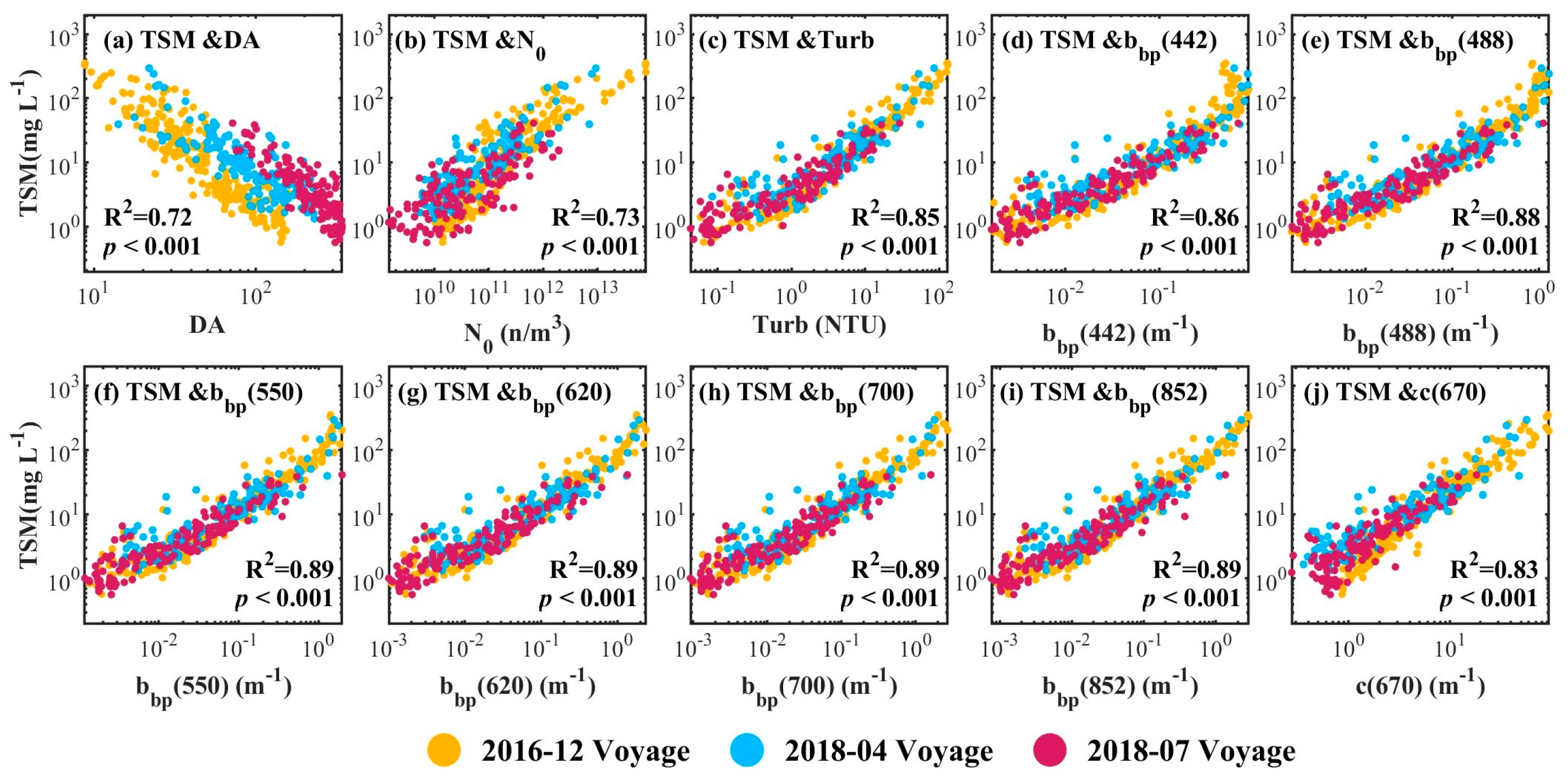
Figure 2. Workflow for estimating TSM vertical profile data from satellite observations.
Remotesensing 16 03736 g002
Figure 3. The TSM vertical distribution in the BSYS: samples of the uniform type (a); samples of the increasing type (b). Schematic diagram of TMS vertical distribution types (c).
Remotesensing 16 03736 g003
Figure 4. Correlation between the TSM concentrations and different bio-optical paraments.
Remotesensing 16 03736 g004
Figure 5. Comparisons between the measured and estimated TSM concentrations in training (a) and testing dataset (b). Solid lines represent the 1:1 line.
Remotesensing 16 03736 g005
Figure 6. Statistics of the TSM vertical type in different seasons across various regions: (a) the whole BSYS; (b) the BS; (c) the NYS; (d) the SYS.
Remotesensing 16 03736 g006
Figure 10. Proportional distributions of the TSM vertical types in the BSYS from January to December: (a) the uniform type; (b) the increasing type.
Remotesensing 16 03736 g010
Figure 12. Monthly distributions of the column-integrated TSM in the BSYS during the period from 2003 to 2021.
Remotesensing 16 03736 g012
Table 1. Coefficient values for the TSM profile reconstruction model.
Parameter a0DAN0Turbbbp (442)bbp (488)
Coefficient3.1040.065−0.026−0.6710.027−1.305
Parameterbbp (5 50)bbp (620)bb p(700)bbp (852)C (670)
Coefficient1.2080.5841.083−0.2630.067
Table 2. Confusion matrix of the field-measured and method-detected TSM vertical types using the TVTC method.
TypeMethod-Detected TypePrecision (%)Dataset
UniformIncreasing
Field-measured typeuniform51985.0%Training
increasing158184.3%
uniform22484.6%Testing
increasing73482.9%
Table 3. Correlations of the diffusion theory model parameters a and b with marine environmental factors and surface TSM.
ParameterDepthWind SpeedSSTSSSTSMsurf
a0.0150.0000.0220.0000.001
b0.0550.0150.0040.0040.000
Disclaimer/Publisher’s Note: The statements, opinions and data contained in all publications are solely those of the individual author(s) and contributor(s) and not of MDPI and/or the editor(s). MDPI and/or the editor(s) disclaim responsibility for any injury to people or property resulting from any ideas, methods, instructions or products referred to in the content.

