Article

Analyzing Temporal Characteristics of Winter Catch Crops Using Sentinel-1 Time Series

by
Shanmugapriya Selvaraj
1,
Damian Bargiel
2,
Abdelaziz Htitiou
1 and
Heike Gerighausen
1,*
1
Julius Kühn Institute (JKI)–Federal Research Centre for Cultivated Plants, Institute for Crop and Soil Science, Bundesallee 58, 38116 Braunschweig, Germany
2
Institut für Landschaftsplanung und Naturschutz, Hochschule Geisenheim University, Rüdesheimerstraße 18, 65366 Geisenheim, Germany
*
Author to whom correspondence should be addressed.
Remote Sens. 2024, 16(19), 3737; https://doi.org/10.3390/rs16193737
Submission received: 25 July 2024 / Revised: 20 September 2024 / Accepted: 4 October 2024 / Published: 8 October 2024

Abstract

:
Catch crops are intermediate crops sown between two main crop cycles. Their adoption into the cropping system has increased considerably in the last years due to its numerous benefits, in particular its potential in carbon fixation and preventing nitrogen leaching during winter. The growth period of catch crops in Germany is often marked by dense cloud cover, which limits land surface monitoring through optical remote sensing. In such conditions, synthetic aperture radar (SAR) emerges as a viable option. Despite the known advantages of SAR, the understanding of temporal behavior of radar parameters in relation to catch crops remains largely unexplored. Hence, in this study, we exploited the dense time series of Sentinel-1 data within the Copernicus Space Component to study the temporal characteristics of catch crops over a test site in the center of Germany. Radar parameters such as VV, VH, VH/VV backscatter, dpRVI (dual-pol Radar Vegetation Index) and VV coherence were extracted, and temporal profiles were interpreted for catch crops and preceding main crops along with in situ, temperature, and precipitation data. Additionally, we examined the temporal profiles of winter main crops (winter oilseed rape and winter cereals), that are grown parallel to the catch crop growing cycle. Based on the analyzed temporal patterns, we defined 22 descriptive features from VV, VH, VH/VV and dpRVI, which are specific to catch crop identification. Then, we conducted a Kruskal–Wallis test on the extracted parameters, both crop-wise and group-wise, to assess the significance of statistical differences among different catch crop groups. Our results reveal that there exists a unique temporal pattern for catch crops compared to main crops, and each of these extracted parameters possess a different sensitivity to catch crops. Parameters VV and VH are sensitive to phenological stages and crop structure. On the other hand, VH/VV and dpRVI were found to be highly sensitive to crop biomass. Coherence can be used to detect the sowing and harvest events. The preceding main crop analysis reveals that winter wheat and winter barley are the two dominant main crops grown before catch crops. Moreover, winter main crops (winter oilseed rape, winter cereals) cultivated during the catch crop cycle can be distinguished by exploiting the observed sowing window differences. The extracted descriptive features provide information about sowing, harvest, vigor, biomass, and early/late die-off nature specific to catch crop types. In the Kruskal–Wallis test, the observed high H-statistic and low p-value in several predictors indicates significant variability at 0.001 level. Furthermore, Dunn’s post hoc test among catch crop group pairs highlights the substantial differences between cold-sensitive and legume groups (p < 0.001).

1. Introduction

The European Union (EU) set an ambitious goal to reduce greenhouse gas (GHG) emissions by 40% in 2030 in compliance with the Paris Agreement [1]. Later, this target was increased to 50–55% under the EU Green Deal, with the ultimate goal of achieving carbon neutrality by 2050 [2]. Under this, in 2020, the European Commission recognized climate change mitigation in agricultural sector as one of the main priorities of the Common Agricultural Policy (CAP) [3]. To successfully align the CAP with climate action, it is essential to understand the mitigation potential of current agricultural practices, as well as the policy measures that could encourage the adoption of promising practices [4]. Within the agricultural sector, catch crops are seen as effective tools for reducing greenhouse gas emissions.
Catch crops (also known as cover crops) are fast-growing crops that are cultivated between the two main crop growing seasons and act as a green soil cover during the winter season. As a part of innovative crop production systems, they offer a wide variety of ecosystem benefits such as preventing nitrogen (N) leaching, soil erosion, and promoting sustainable land use by enriching biodiversity and soil organic matter [5,6]. Unlike other main crops, catch crops are not cultivated for economic benefits; hence, these crops are plowed directly into the soil to act as fertilizer for upcoming main crops. In European conditions, catch crops are generally grown as winter cover crops during fall (after the harvest of main crop) between the months of August and February. Catch crops are either cultivated as pure stands or seed mixtures. The most commonly grown varieties are white mustard, oilseed radish, phacelia, niger, sunflower, clover, vetch and lupine [7].
Growing catch crops has attained greater importance in the last decade due to their potential role in climate change mitigation and soil protection. Under favorable conditions, they are key for soil carbon sequestration and reducing emissions from agricultural soils, thereby contributing to diversification in crop rotations [8,9]. In view of this potential for climate change mitigation, spatially explicit, regular and timely monitoring of catch crops is required as a basis for site-specific assessment and decision support for crop rotation practices. Conventionally, crop information and areas were recorded using field-based inspection and farmer’s surveys. These approaches are often expensive, labor-intensive, time-consuming, spatially generalized, and are not feasible for larger areas [10]. Recently, the unprecedented availability of Sentinel-1 and -2 data that are freely accessible with high spatial and temporal resolution has facilitated consistent time series for temporal monitoring of crops [11,12]
Several previous studies have focused on mapping main crop types [13,14,15], crop sequences [16], and crop rotation practices [17,18] using optical and radar data to a large extent. However, only a few of these studies dealing with catch crop mapping using satellite data can be found in the literature. For instance, Schulz et al. [19] investigated the dense time series of NDVI from Sentinel-2 data and proposed a classification scheme to identify catch crops at parcel level in Germany. The results showed that distinguishing between different catch crop types was not possible because of similar NDVI response to all catch crop types. In another study, spectral bands and indices from Landsat-8 time series were used to broadly identify the winter cover crop growing areas [20]. Many other studies were also restricted to optical remote sensing for mapping cover crops [21], estimating its biomass and percent ground cover [22,23,24]. All these previous studies have highlighted significant challenges in using optical data to monitor cover crops, particularly due to the difficulty in obtaining clear satellite images during autumn and winter months, a critical issue since the entire growth period of catch crops coincides with these cloud-prone months. Additionally, differentiating among different cover crop types and between winter main crops, random vegetation, and weeds is challenging due to their spectral similarities. All these constraints could affect the applicability of the findings in varying geographical and climatic conditions. Another major challenge with optical sensors is the problem of low irradiance and large sun angle variation observed during winters, especially in higher altitudes [25]. On the other hand, SAR (synthetic aperture radar) observations such as those provided by Sentinel-1 can acquire cloud-free images regardless of the weather, at any time of day or night. Moreover, radar echoes possess unique sensitivity towards geometric structure and dielectric constant of crops [26].
Many previous studies have proved the existence of direct sensitivity between various SAR parameters and main crops [27,28]. A number of studies found that the backscatter coefficients extracted from multitemporal SAR data have the potential to identify different crop types [29,30]. Radar response to crops is largely polarization-dependent, and studies have successfully demonstrated that the exploitation of multipolarization modes performs better for crop mapping [31,32]. Crop structure and vegetation water content vary throughout the growing cycle (from plant emergence to senescence), and also differ with crop types. Hence, crops exhibit different scattering responses with respect to crop type (erectophile or planophile), phenological stage, and polarization mode [33,34], which in turn are reflected in the backscatter behavior. Understanding and capturing these temporal variations is crucial for crop discrimination. In this context, a number of studies have explored SAR data to study the temporal pattern of main crops (paddy, wheat, barley, rapeseed, corn, and so on) to a large extent [30,35,36,37].
To our knowledge, the understanding of temporal behavior of catch crops in the radar domain is not well established and, so far, no studies pertaining to this can be found in the literature. Our research aims to fill this research gap by investigating the distinct characteristics and patterns of catch crops in the radar domain. In order to derive methods using dense time series SAR data for catch crop classification, there is a need to study the temporal behavior of different catch crop types. SAR data are particularly useful due to their unique backscatter behavior, which varies significantly among crop types based on leaf type, crop structure, and moisture content, providing an opportunity to distinguish between different catch crop types. Hence, our study aims to assess the potential of Sentinel-1 time series by exploiting the most significant SAR parameters such as VV, VH backscatter, ratio, dpRVI (dual-pol Radar Vegetation Index), and VV coherence to investigate the temporal patterns of winter catch crops. In addition, we also incorporate the main crop temporal signatures in the profile study to analyze and compare their behavior with catch crops. We then develop a set of descriptive features from these parameters, specific to catch crop identification, and statistically evaluate its significance using the Kruskal–Wallis H-test and Dunn’s post hoc test.

2. Materials and Methods

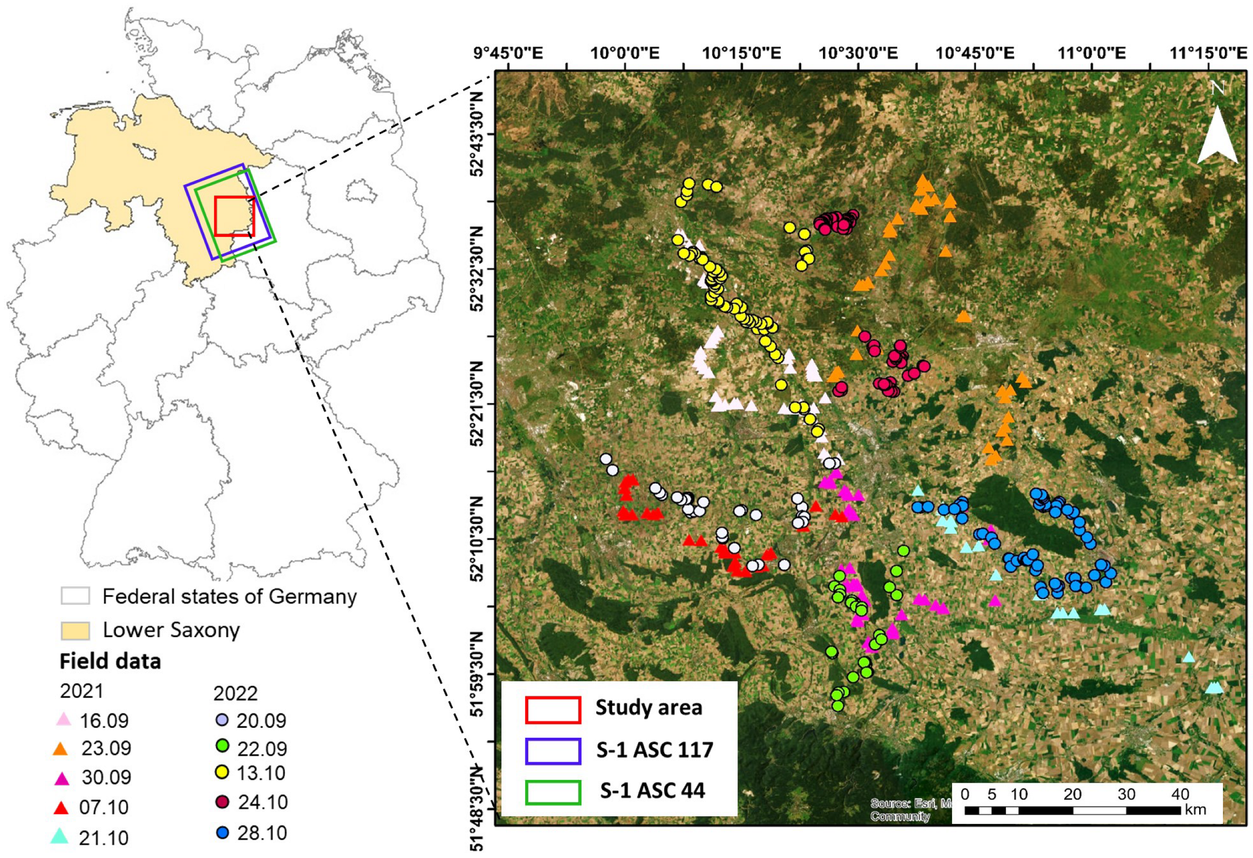
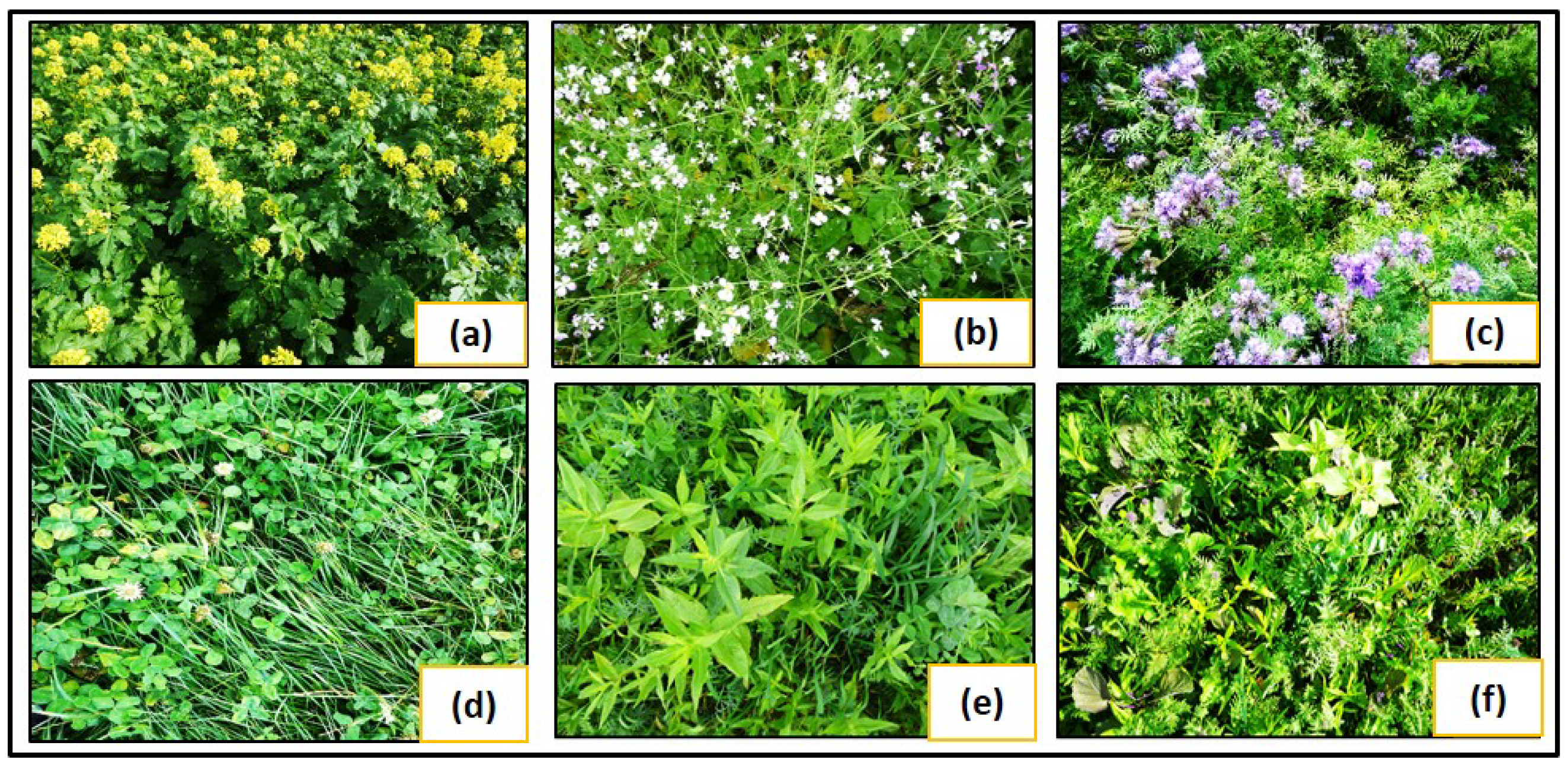
2.1. Study Area and Ground-Truth Campaigns
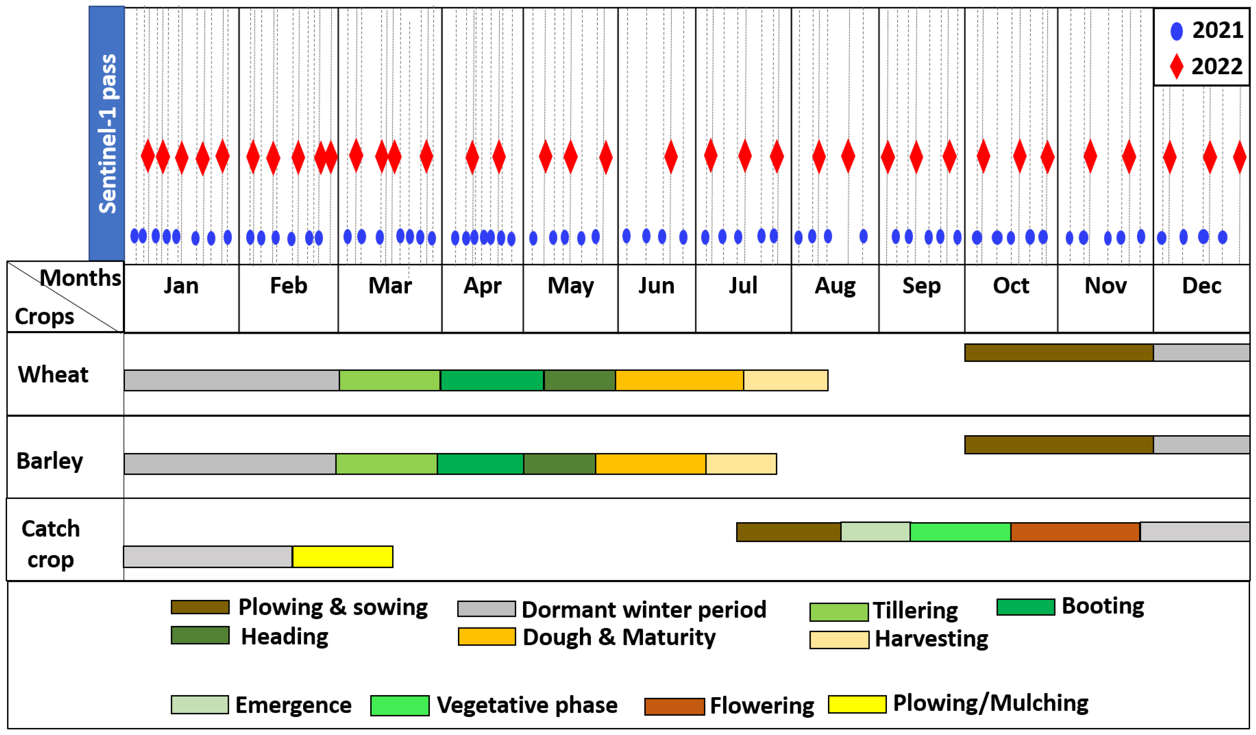
The test site covers the greater Brunswick region, which is located in the federal state of Lower Saxony (LS), Northern Germany. The area receives approximately an average yearly precipitation of about 703.5 mm. The soil type in the region is characterized by fine sandy loam soils [38]. The total arable agricultural land constitutes approximately 1,864,964 hectares, with permanent cropland accounting for about 18,094 hectares and permanent grassland accounting for about 734,634 hectares [39]. The average field size in the Greater Brunswick region is around 3.36 ha, and was computed by taking account of the Integrated Administration Control Systems (IACS) field parcels. In situ reference data on catch crops was collected in five field campaigns in 2021 and five in 2022 during the peak growing season of catch crops in Germany, that is, from mid-September to mid-October. The dates on which the field campaigns were conducted can be seen in Figure 1. In total, 306 and 289 agricultural fields with catch crops were inspected in the year 2021 and 2022. For each field, catch crop type or seed mix was determined, field photographs were recorded (Figure 2), and parcel boundaries were extracted.
Based on the N content and winter behavior, we broadly classified the catch crops into three categories, such as cold-tolerant, cold-sensitive, and legumes, for further analysis. For instance, cold-tolerant ones can withstand freezing temperatures and hold nitrogen throughout the winter and release it slowly, making it available for the upcoming main crop in the spring. Cold-sensitive catch crops typically die off early in the winter (around December) and release nitrogen early into the soil. With increased precipitation during winter, this can lead to nitrogen leaching and potential environmental pollution. However, this will be useful when sowing winter main crops (wheat, barley) during October or November. Legume catch crops have the unique ability to fix atmospheric nitrogen and thereby contribute more nitrogen fixation than other groups. This classification scheme aids in selecting appropriate catch crops for different agricultural scenarios to maximize environmental and economic benefits. The detailed overview of groupings and number of samples collected for each catch crop are given in Table 1. The main crop information for the respective catch crop parcels for the years 2021 and 2022 were extracted from IACS data, with which payments are made to farmers under the common agricultural policy (CAP). Using Land Parcel Identification System, IACS data provide field-level information on most of the agricultural parcels with detailed information on the field area and main crop type on a yearly basis [40]. IACS is widely recognized data that are utilized across Europe for agricultural monitoring and subsidy management. The accuracy of IACS data is ensured through rigorous administrative checks and field inspections conducted by national authorities. These checks involve cross-referencing with other datasets and on-site inspections to validate the accuracy of the reported crop types and land use. Moreover, the data are updated annually, reflecting the most current land use and cropping patterns. This makes IACS data an ideal reference dataset for winter non-catch-crop parcels. However, it only contains farmer fields that qualify for European Union subsidy payments [14,41]. In our study area, analysis of IACS parcels reveals that winter wheat and winter barley are the two dominant main crops grown in this area before catch crops.

2.2. Satellite Data

Here, we exploited both ground range detected (GRD) and single-look complex (SLC) formats of the Sentinel-1 (S-1) SAR dataset from the German cloud computing platform CODE-DE [42]. The S-1 images were available in interferometric wide (IW) swath mode with two polarizations (VV and VH). Both GRD and SLC images were resampled and are available in 10 m resolution with the central incidence angle of about 41°, which is ideal for crops as it increases the path length through vegetation and results in more vegetation backscattering [43]. More details about the dataset can be seen in Table 2. Since earlier studies indicated that morning dew on crop canopy has a severe impact on SAR backscatter [44,45,46,47,48], we utilized Sentinel-1 images (orbit 117 and 44) only from the ascending pass (ASC) acquired at approximately 5:00 p.m. local time. The Sentinel-1 satellite passed over the study area during 2021 and 2022 covering the growth cycle of main and catch crops that are depicted in Figure 3. A total of 65 and 38 S-1 images were used in 2021 and 2022, respectively. SAR is highly sensitive to moisture changes [49]; therefore, we also considered daily precipitation and temperature data from the German Meteorological Office or Deutscher Wetterdienst (DWD) in our study [50]. These datasets are available at 1 × 1 km spatial resolution as regional averages that can be accessed from the Julius Kuehn Institute (JKI) datacube through web services such as Web Coverage Services (WCS) [51].

2.3. SAR Data Preprocessing

Both GRD and SLC data-products were preprocessed using the Sentinel-1 SAR preprocessing chain established by Julius Kuehn Institute (JKI) [52]. Sentinel-1 preprocessing uses the PyroSAR [53] Python library for multiprocessing by accessing the graph processing tool from the SNAP Sentinel-1 toolbox. Firstly, the GRD amplitude images were subjected to thermal and border noise removal to remove the border artifacts and non-values. Then, orbital file correction was performed to update the orbital files with precise orbital vectors from meta data. This was followed by radiometric calibration, speckle filtering (5 × 5 Refined Lee), and terrain correction using a Copernicus 30 m digital elevation model (DEM) to generate gamma nought backscatter coefficients ( γ VV 0 , γ VH 0 ) (in dB). Subsequently, we subtracted γ VH 0  from γ VV 0 to generate the cross-polarization ratio ( γ 0 VV / VH ) images in dB. Hereafter, the parameters are referred as as VV, VH, and VH/VV.
As the SLC data were acquired in TOPSAR (Terrain Observation with Progressive Scans SAR) mode, the processing chain of the SLC was slightly different from GRD images. After applying orbit file correction, the processing chain starts by applying the TOPSAR split function that splits the entire image into three sub-swaths (IW1, IW2, and IW3) to ensure a uniform signal-to-noise ratio (SNR). This was followed by calibration and deburst operation, which merges the bursts in the azimuth direction to obtain a continuous image for further analysis. We then generated polarimetric C2 matrix and applied multilooking to generate square pixels. To suppress the inherent speckles, an adaptive polarimetric speckle filter such as Refined Lee with window size 5 × 5 was applied to the images. Refined Lee is highly suitable over agricultural areas as it suppresses the noise without comprising the image details and has a higher Equivalent Number of Looks (ENL) [54]. Finally, we generated the terrain-corrected dual-pol Radar Vegetation Index (dpRVI).
Unlike RVI, which utilizes only backscatter intensity from polarization channels, dpRVI is generated by taking account of dominant scattering component (in terms of Eigen values from C2 covariance matrix) and polarization channels and then normalized with total power (Span) [55], as denoted in Equation (1). dpRVI ranges from 0 (no vegetation) to 1 (healthy vegetation) and can monitor growth dynamics, health, and condition of crops. Comparing with other intensity only based-RVIs, dpRVI showed better results for diverse crops and can overcome the problem of saturation [56]. dpRVI is mathematically defined as follows:
d p R V I = 1 m · β
where m is the the degree of polarization, which is generated from the C2 covariance matrix and represented as
m = 1 4 | C 2 | Tr ( C 2 ) 2
Tr is the sum of diagonal elements, | . | matrix determinant and β (Dominancy of scattering) is given as
β = λ 1 Span
The combined use of m and β enables us to capture scattering mechanism variations with respect to phenological stages, as both parameters have different sensitivity to crop growth. For coherence generation, soon after applying orbital file correction, co-registration was performed using the back-geocoding method followed by Enhanced Spectral Diversity (ESD) to improve the quality of co-registration. The images were again subjected to deburst/merge operations and, finally, coherence for each image pair was computed. The images were finally multilooked and terrain-corrected for further analysis. Interferometric coherence is mathematically defined as the magnitude of the complex cross-correlation of two SAR images (either mono-static or bi-static SAR images) [57] and is represented mathematically as follows:
μ 0 = | S 1 S 2 | S 1 S 2 S 1 S 2
where S refers to the complex conjugate of S 1 and S 2 (SAR image pairs) and <> refers to the collective average. In general, μ 0 estimates the phase stability between two SAR images and ranges between 0 and 1, where 0 refers to complete decorrelation and 1 refers to perfect correlation. The coherence decreases when the Earth’s surface undergoes some changes between two SAR acquisitions (soil moisture changes, ongoing urban constructions, and so on) and, also, coherence considerably decreases when the return signal has more volume scattering, which is true in areas of dense forests and croplands [58].

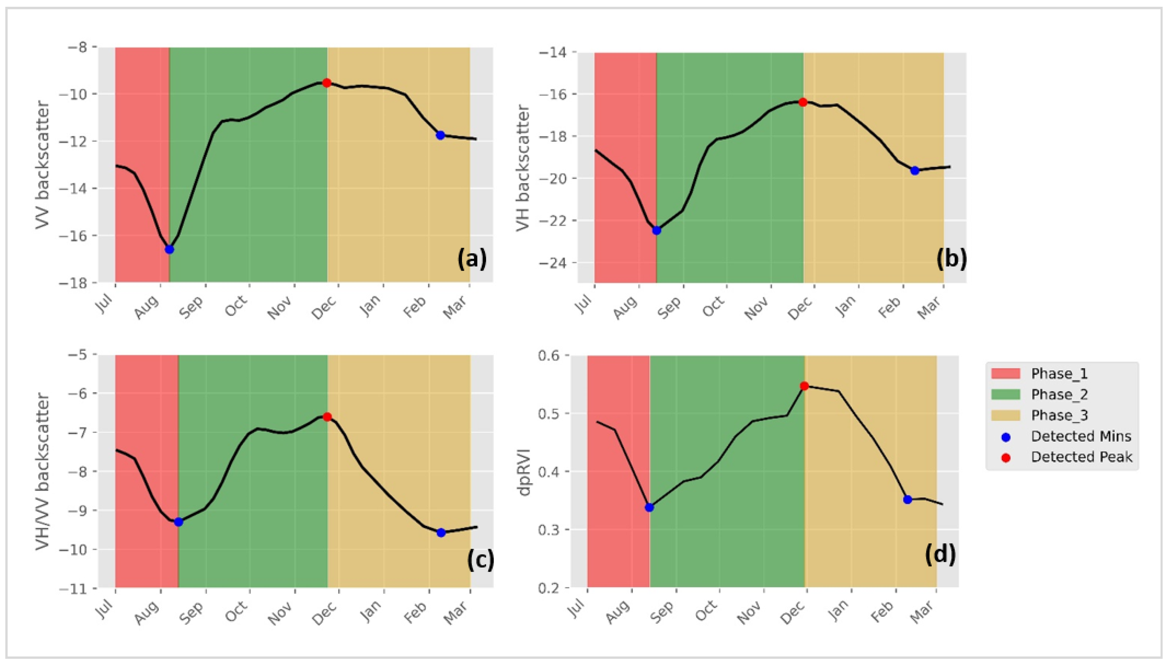
2.4. Temporal Profile Analysis

For each catch crop parcel, the temporal mean values of VV, VH backscatter, ratio, DpRVI, and coherence were extracted and grouped according to the catch crop categories with corresponding pre-crop.The mean value provides a straightforward and representative measure of central tendency, which is particularly useful for understanding the general behavior of the crop responses over time [30,36,59]. Time series were plotted for main and catch crop cycle and temporal signatures were visually interpreted to understand the pattern variations and trend (Section 3.1, Section 3.2, Section 3.3 and Section 3.4).
Since winter crops such as winter oilseed rape and winter cereals are sown during late autumn and they overlap with the catch crop growing phase, we also extracted and compared their temporal behavior with the catch crop to examine the sowing window differences. Random vegetation (weeds or seedlings emerge from previous crops) on fallow fields, as well as frequent tillage or plowing activities, can often be a source of misclassification. Thus, we extracted signatures from fallow fields and compared them with catch crop temporal patterns. As the same winter crops were grown during the years 2021 and 2022, we took the mean profiles from the year 2021 for comparison. Since the coherence measurements are more sensitive to management practices rather than crop phenology and development [60], we opted to exclude coherence data for this analysis. Instead, we focused on VV, VH backscatter, ratio, and dpRVI to better understand the differences in radar response between these classes. The winter main crop parcels and fallow fields were extracted from IACS data.

2.5. Descriptive Features Extraction

Based on our time series analysis, we developed and extracted a number of descriptive features from VV, VH, VH/VV, and DpRVI, which seem to be highly effective for distinguishing and monitoring the various studied catch crops. To achieve this, the entire profile of a given catch crop was separated into three temporal phases by automatically identifying three temporal breakpoints, which are represented by local extrema (composed of a peak and and its two neighboring left–right local minima) over each curve, as shown in Figure 4. This approach, based on the technique used to define the crop’s temporal domain as described in [61,62], automatically and effectively characterizes the periodicity of catch crops by identifying temporal breakpoints that likely separate phenological phases in the time series for each catch crop field. More specifically, the peaks (maximum values) in the backscatter time series were identified using a peak detection method with a threshold value. When multiple peaks were detected within a single-temporal profile, we used the prominence (height of the peak) of each peak to identify the most significant one. Similarly, the two neighboring minima (lowest points) surrounding the detected peak were identified using a similar minima detection method, which helps in accurately segmenting the time series into the three mentioned temporal phases.
The first phase denotes the ripening and harvest phase of main crops and subsequent sowing of catch crops. It spans from the beginning of the time series until the first detected local minima. The second phase extends from the first detected local minima to the peak position. It encompasses the primary growth period, including maturation, where the crops reach their peak vegetative growth. The characteristics observed in this phase provide insights into the crop’s health and growth dynamics. The third phase covers the period from the detected peak to the subsequent minimum value. It corresponds to the dormant winter period and the eventual harvest of catch crops. This phase is indicative of the crop’s senescence and post-maturity behavior of different catch crop groups. These phases were defined in reference to the work by Schulz et al. [19]. To ensure the robustness and predictiveness of our analysis, we aggregated all profiles from the years 2021 and 2022 for extraction of descriptive features. This consolidation allows for a more representative and predictive assessment of the derived predictors. Since we are developing the descriptors specific to catch crops, we only included the time series from July to March, which is the cultivation period of catch crops.
Similar to NDVI, the dpRVI index indicates the phenology and health of the plant [63]. Thus, different phenological features have been extracted based on the generated DpRVI time series using the dynamic threshold method for each temporal phase, such as the Start_of_ Season (SOS), End_of_ Season (EOS), and Start of senescence, which we found to have high importance for catch crops. For more information about the mathematical base of the abovementioned phenology metrics computation and their settings, readers can refer to [64].
In addition to the previous phenological features, 19 other multitemporal statistical features specific to catch crops were defined. In total, 22 descriptive features encompassing phenological and statistical features were proposed in this study. The ultimate goal of using them was achieving a high information rate for distinguishing catch crops from main crops and differentiating between various catch crop classes.The detailed descriptions about all the used features can be found in Table 3.

2.6. Kruskal–Wallis H-Test

Here, we performed the Kruskal–Wallis H-test, a nonparametric statistical test to compare the variance of extracted descriptors among multiple catch crops to determine whether they are significantly different to each other. The Kruskal–Wallis test does not require the assumptions of normality and homogeneity of variances, making it ideal for our dataset with varying distributions and potential outliers [65]. This ensures a more reliable comparison of the groups. This test generates two important metrics, the H-statistic, and a corresponding p-value. The H-statistic measures the variance of the ranks among groups. A higher H-statistic indicates greater differences in the distributions of the groups. The p-value indicates the probability of obtaining the observed H-statistic if the null hypothesis (i.e., all group distributions are equal) is true. If the p-value is less than the significance level (generally < 0.05), the null hypothesis is rejected, indicating significant differences in the distributions of the groups [66].
After extracting the 22 descriptors for each catch crop parcel, we conducted the Kruskal–Wallis test in two ways: first, as individual crop-wise (comparing each crop distribution with others), and second, by grouping the catch crops into cold-tolerant, cold-sensitive, and legume categories. For each crop and descriptor, the H-statistic and p value were given as *, **, *** indicating 0.05, 0.01, and 0.001 level of significance in Appendix A, Figure A1; and for the group-wise test, the results were indicated in Table 4.

2.7. Dunn’s Post Hoc Test

For the group-wise comparisons, where significant differences were found in the Kruskal–Wallis test, Dunn’s post hoc test with Bonferroni correction was applied to identify which specific groups differed [67]. This step is crucial because the Kruskal–Wallis test can only indicate that at least one group is different, but it does not specify which pairs of groups are different. The Bonferroni correction is applied to adjust the p-values for multiple comparisons to control the overall type I error rate. Without this correction, conducting multiple comparisons could inflate the probability of incorrectly rejecting the null hypothesis (false positives). The p-values of Dunn’s test were marked with *, **, and *** to indicate significance levels of 0.05, 0.01, and 0.001, respectively, as shown in Table 5.

3. Results

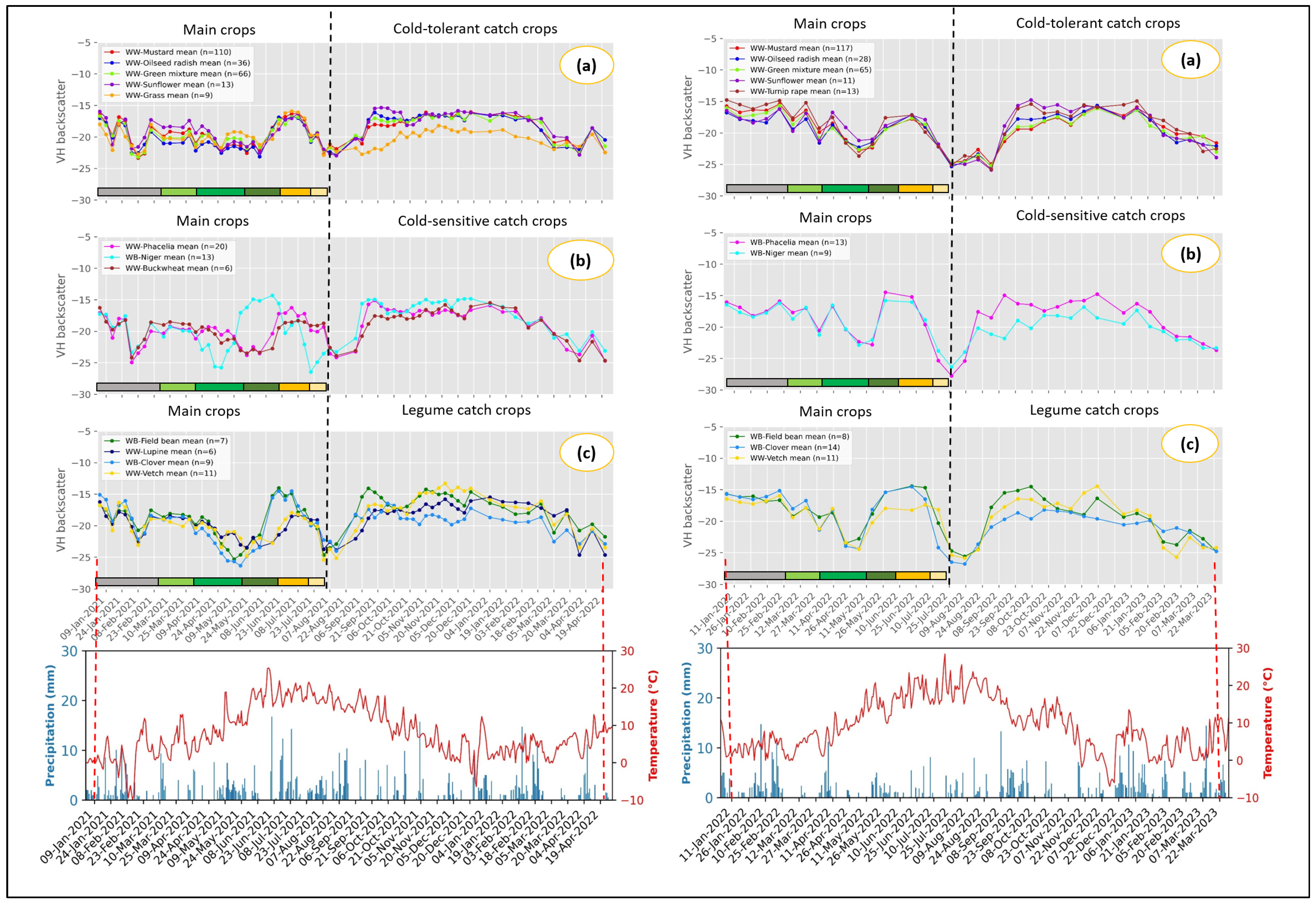
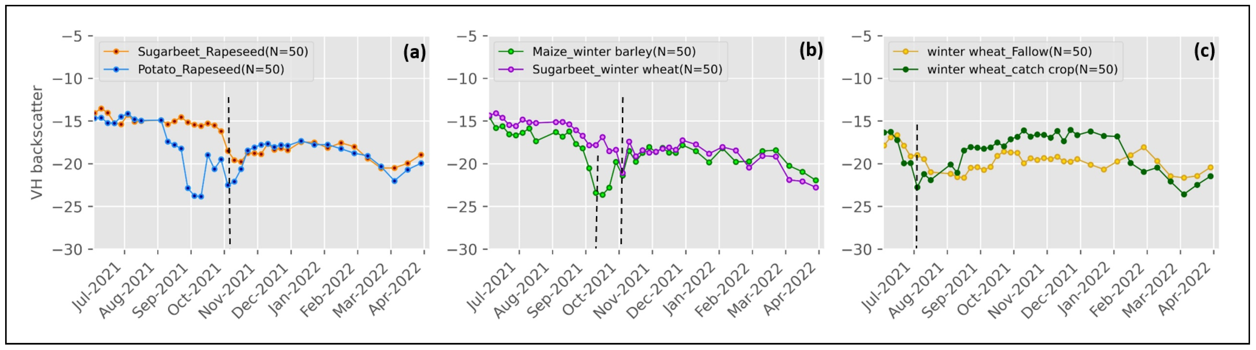
3.1. S-1 VV, VH-Backscatter

From our analysis of IACS data for catch crop parcels, we found that winter wheat (hereafter named as WW) and winter barley (hereafter named as WB) were the two dominant pre-crops cultivated in this region. When looking at the temporal profiles of main and catch crops in Figure 5 and Figure 6, one can notice a distinct and unique pattern for catch crops, and this differs entirely from main crops. For cold-tolerant varieties, WW is the most common main crop. For cold-sensitive varieties, mostly WB is the pre-crop as WB is harvested little early than WW and this favors early sowing of cold-sensitive varieties. Since the cold-sensitive crops cannot withstand low temperatures and they die off just below freezing temperature, early sowing is preferred for large biomass development. Among legume catch crops, for field bean and clover, WB is the pre-crop, and for vetch and lupine, WW is the pre-crop.
When looking at the main crop profile for both years, one could notice a stable backscatter from January to February in VV and VH, as the crop was in a dormant winter phase and there was no active vegetation growth or changes. Most of the changes observed during these months are purely due to changes in soil moisture and roughness. The strong and abrupt dip in VV and VH backscatter during February in 2021, regardless of crop type, was due to frost conditions, which was confirmed by the temperature analysis obtained form DWD, shown in Figure 5 and Figure 6. During March, both WW and WB enter into the tillering stage, where the crop just starts to produce tillers; hence, no prominent changes were observed in backscatter. During April and the beginning of May (when the crop was in stem elongation and booting stage), one can generally notice a decrease in VV and VH backscatter for both WW and WB. During this phase, the cereals start to develop stems, stalks, and flag leaves, which in turn results in a Leaf Area Index (LAI) crop percent cover, and height to reach maximum. Due to these complex phenomena, the VV backscatter reaches a minimum due to maximum signal attenuation observed in the canopy and underlying soil during this stage.
Following this, in mid-May, VV and VH backscatter increase considerably, and this was related to heading stage. This is when the plant develops ear heads and awns and, therefore, fresh biomass increases further. Now, due to a dense canopy architecture with 100 percent crop coverage, returned radar echoes are highly dominated by vegetation and not by the underlying soil. Note that a characteristic difference between the WW and WB profiles can be observed during the heading stage. One can see a very steep increase in backscatter values of around 8 dB in VV and 14 dB in VH for WB fields, which was absent in WW. This can be attributed to the bending of ear heads in WB from vertical to horizontal orientation [68]. In WW, this phenomena is noticed only during the late ripening phase, and by this time, WW have already dried and have low vegetation water content (VWC); therefore, no remarkable changes were noticed in backscatter. During the dough and maturity stages, VV and VH backscatter slowly start to decrease due to the decrease in chlorophyll and VWC, and then they reach the minimum during the harvest (end of July).
Among the cold-tolerant catch crops (Figure 5a), grass has lower VV backscatter than other catch crops and this is due to the vertical structure of grass. In the VV profile, after December, the VV backscatter contribution from grass fields considerably increased compared to other crops, and this was absent in the VH profile (Figure 6a). This can be attributed to soil effects (roughness and moisture), which are more dominantly visible in VV than VH. In both years, sunflower has higher VV and VH backscatter than other crops, as sunflower is a broad-leaved, tall, and high-biomass crop; hence, it contributes to high backscatter. Similarly, in 2022, turnip rape also had high backscatter, and this is because of its planophile nature having broad leaves spread along the horizontal direction. Also, there are some differences observed in the sunflower, radish, mustard and green mixtures in the VV and VH backscatter during the early stages. After these, all the crops follow the same pattern and profiles are found to be mixing with each other. After December, interestingly, the VV backscatter for green mixtures started to increase in both years (Figure 5a).
Considering the cold-sensitive category (Figure 5b), niger was planted a little earlier than phacelia and buckwheat in 2021, which in turn resulted in more biomass development in niger and, therefore, high backscatter. This is due to the earlier harvest of WB than WW. In cold-sensitive catch crops (Figure 5b and Figure 6b), VV and VH backscatter decreases steadily and steeply after December compared to others; this may be due to the early die-off of cold-sensitive catch crops. Among legumes (Figure 5c and Figure 6c), clover has low VV and VH backscatter contribution for both the years due to its less competitive growth nature, resulting in low biomass. Similarly, field bean has higher backscatter than others because of its high vigor and biomass development. The slight increase in VV backscatter observed in vetch and lupine after December could be associated with soil surface changes.

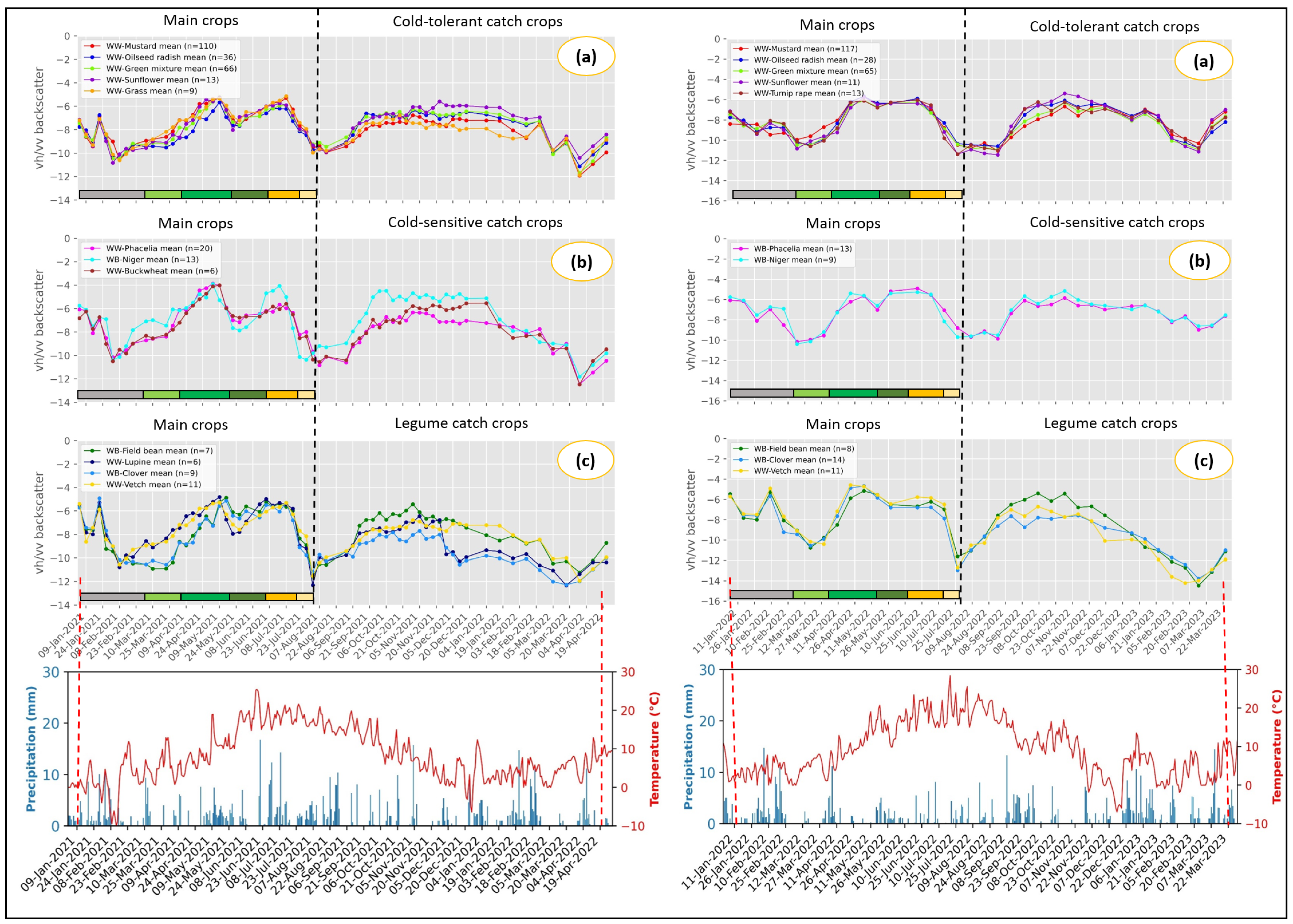
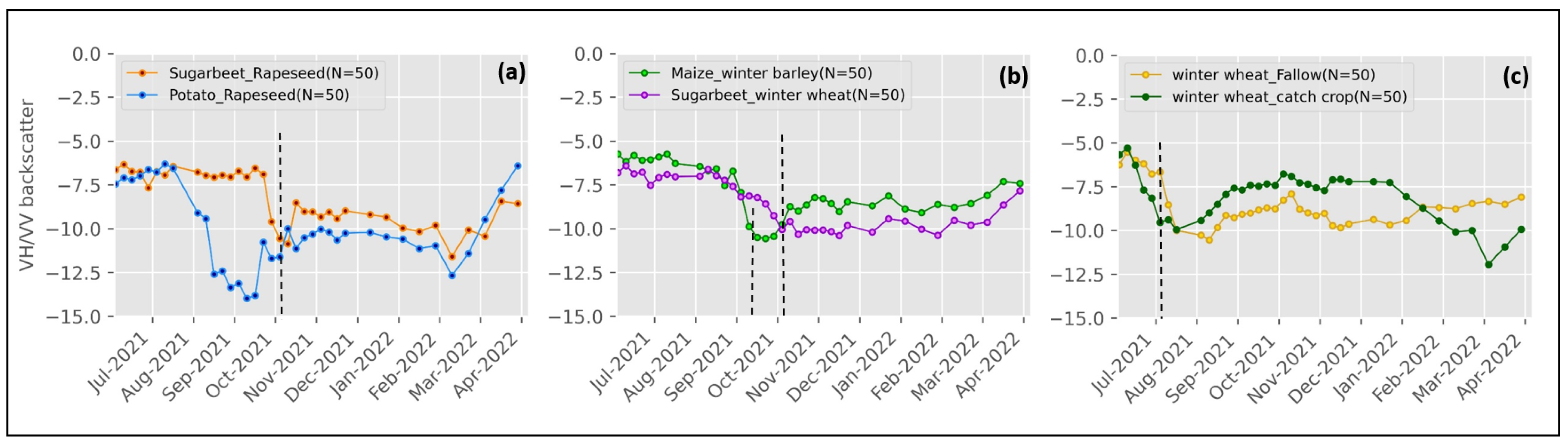
3.2. S-1 VH/VV Backscatter

Considering the main crops in Figure 7 for both the years, the VH/VV backscatter ratio starts to increase from the tillering stage in March, remains high, and decreases during the harvest in July. This can be clearly seen in both the years 2021 and 2022. Interestingly, a slight dip in VH/VV backscatter was observed during the end of booting stage for both WW and WB.
This pattern was specific to winter cereals and differs significantly from the profiles observed in catch crops. It underscores the high correlation and sensitivity of VH/VV backscatter to the biomass of crops. In contrast to VV and VH backscatter, which exhibit high sensitivity to phenological and canopy structural changes, VH/VV backscatter was found to be highly sensitive to the growth cycle of winter cereals.
For catch crops, VH/VV backscatter increases with crop emergence in August, remains high, and subsequently decreases during the harvest of crops in February. In the cold-tolerant category (Figure 7a), all crops follows a similar pattern, with backscatter decreasing towards the end of February. For cold-sensitive crops, VH/VV backscatter decreases a little earlier than other categories, which is particularly evident in the year 2021 (Figure 7b). This may be due to early die-off of crops or due to some management activities carried out in the fields. In the case of legumes (refer to Figure 7c), a marked decline in backscatter was noted for lupine and clover at the onset of December. Towards the end of February, VH/VV exhibits a noticeable rise, independent of specific crop varieties. This may be attributed to spontaneous vegetation growth following the removal of catch crops or the resurgence of previously sown seeds.

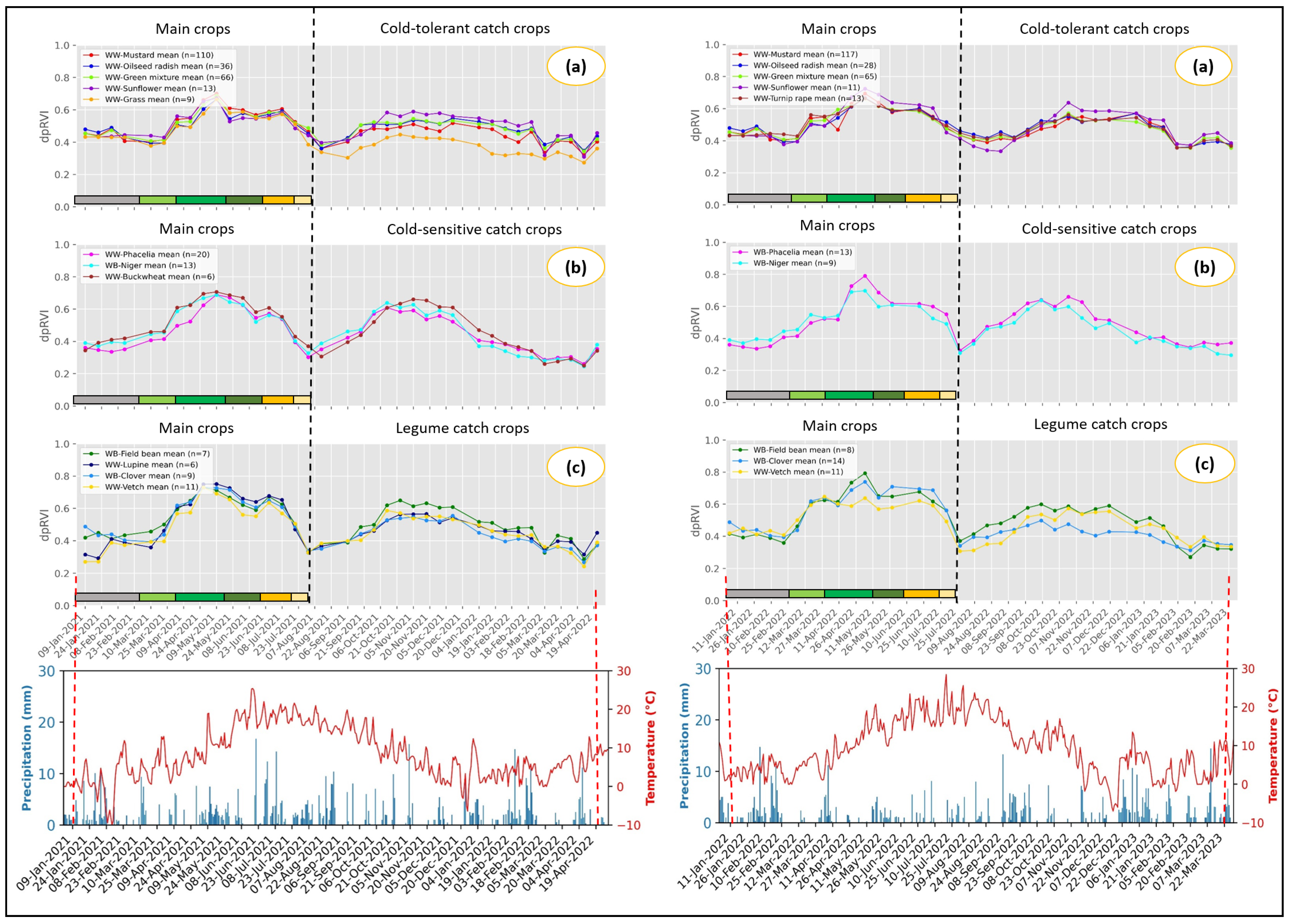
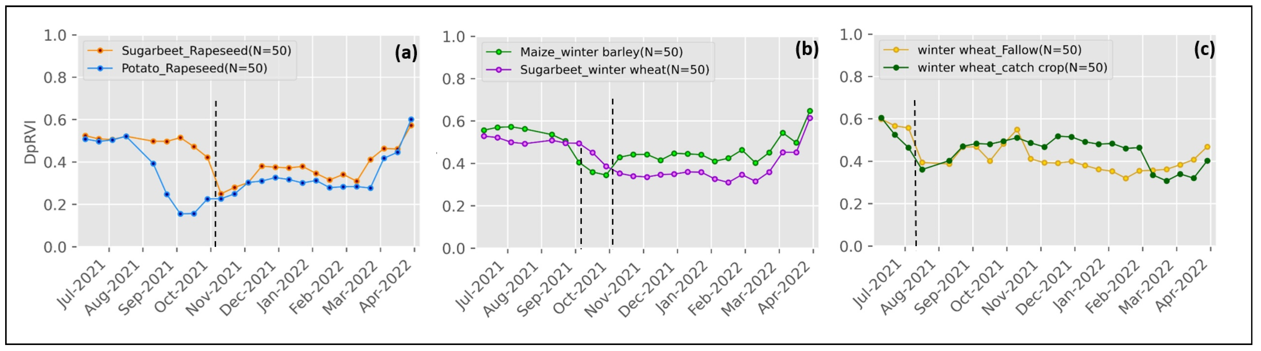
3.3. Dual-Pol Radar Vegetation Index

Since both WW and WB exhibit similar canopy architecture (vertical distribution of canopy elements) and phenological cycles, both cereals have similar dpRVI response. When examining the dpRVI values for the main crops in Figure 8, it was observed that the dpRVI values stay low and stable at around 0.4 until the end of February (no active vegetation growth). By mid-March, when the WW and WB start to tiller and progress further, dpRVI also starts to increase and reaches around 0.6. During the booting stage, the dpRVI spikes to 0.7, indicating an increase in biomass accumulation due to further development of leaves, stems, and stalks.
Notably, dpRVI decreases to 0.5 during the heading stage, despite a further increase in biomass and high plant density. After this, dpRVI slightly increases to 0.6 during the early dough stage, and after this, a gradual decrease was observed during the ripening phase. Finally, dpRVI declines to 0.3 at the harvest stage. This comprehensive analysis delineates the dynamics of dpRVI as a reliable indicator of biomass accumulation and phenological phases in winter cereals.
Unlike main crops, catch crops exhibit no abrupt changes in dpRVI values corresponding to phenological stages, and this is primarily owing to their planophile canopy architecture. Among cold-tolerant varieties (Figure 8a), grass has considerably low dpRVI values of about 0.4 until December, after which the values decline to 0.3 throughout the winter. Conversely, other varieties such as mustard, radish, green mixtures, sunflower, and turnip rape have a stable dpRVI values ranging from 0.5 to 0.6 throughout their entire growth cycle.
For cold-sensitive varieties (Figure 8b), the dpRVI values peak to 0.6 and above during the peak vegetative phase. This is due to the early sowing of cold-sensitive varieties, resulting in high biomass development. As cold-sensitive varieties approach their peak winter phase by the end of December, dpRVI values steadily decrease below 0.4. This is due to early die-off of crops unable to withstand freezing temperatures. This trend of steady decline in dpRVI values was not observed in cold-tolerant and legume species. This pattern validates the early die-off of cold-sensitive crops compared to others, serving as an indicator for distinguishing cold-sensitive varieties. Among legumes (Figure 8c), field bean stands out with high dpRVI values of around 0.6, attributed to its substantial biomass and vigor compared to vetch, clover, and lupine.

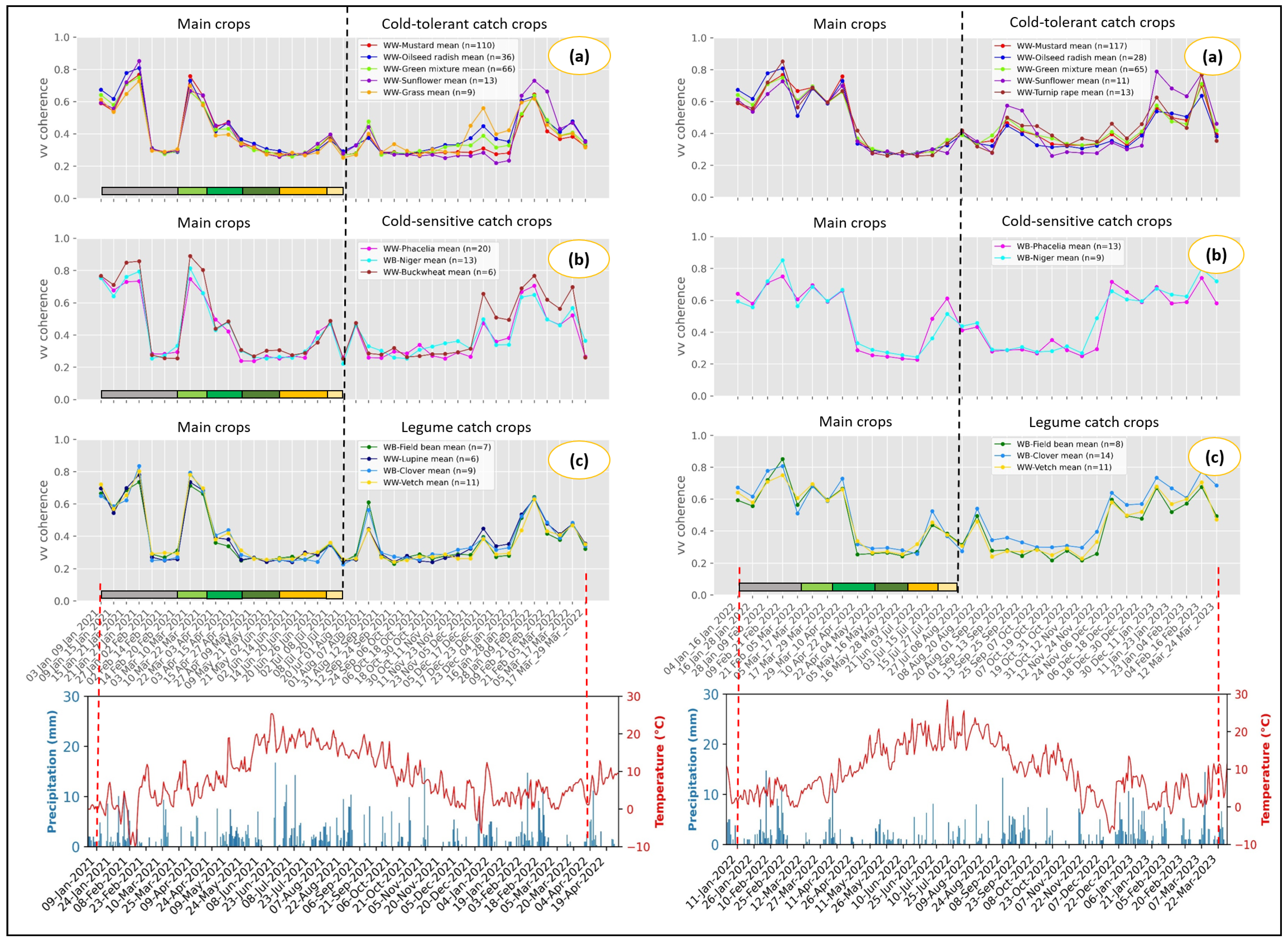
3.4. S-1 VV-Coherence Analysis

In this study, we utilized Sentinel-1 VV coherence data acquired during the ascending pass (orbit track-117) to analyze the main crops and the different catch crop types for the years 2021 and 2022, as illustrated in Figure 9. In the context of multitemporal analysis, interferometric coherence follows a opposite pattern compared to SAR backscatter concerning the crop growth cycle. Our findings reveal that coherence values are lower (ranging between 0.2 to 0.3) during the peak crop growing period for both main and catch crops.
For main crops (WW and WB), one can observe high coherence of about 0.5 to 0.9 during the winter dormant phase and tillering phase, characterized by minimal changes in the Earth’s surface due to inactive crop growth. Also, the sudden dip in coherence values (0.2) during February 2021 is associated with moisture changes. After that, coherence values drop to around 0.2 during the booting stage when the crop starts to actively grow and develop. Subsequently, a sharp increase in coherence values above 0.5 was observed when the main crop is nearing the ripening and harvest stage and also during tillage, plowing, and sowing of catch crops.
Unlike main crops, the coherence pattern for winter catch crops is different and provides lot of insights. A slight increase in coherence can be observed during the early emergence and leaf development stages of catch crops, as expected, given the limited volume contribution from the crop canopy during these initial phases. When the catch crop enters the active vegetative phase and once the ground is completely covered with vegetation, coherence values remains low (0.2 to 0.3) due to pronounced volume scattering effects. The coherence values then exhibit a type-dependent increase, commencing around November for cold-sensitive crops (Figure 9b) such as phacelia and niger, and from late December for cold-resistant crops (Figure 9a) like mustard, radish, and sunflower, and legumes (Figure 9c) such as field bean, lupine, vetch, and clover. This increase in coherence values indicates a cessation of further growth or development in catch crops due to low temperatures, effectively marking the onset of the dormant phase that persists throughout the winter.

3.5. Comparison of Temporal Patterns of Winter Main Crops and Fallow with Catch Crop

In Figure 10 and Figure 11, mean VV and VH backscatter responses of winter main crops, fallow, and catch crops are depicted. The profiles indicate that there is a considerable difference in the calendar dates of the catch crop and main crop. Considering Figure 10a and Figure 11a, the sowing period for rapeseed is predominantly observed in October, which is indicated by a prominent dip in VV and VH backscatter. Among winter cereals, (Figure 10b and Figure 11b), it is observed that winter barley is sown a little earlier (September) than winter wheat (October). This is due to the early harvest of pre-crop maize compared to sugar-beet. Lastly, in Figure 10c and Figure 11c, the catch crops are sown very early, around July, compared to the main crops. Fallow fields follow the random pattern and have low backscatter intensity compared to other crops. Also, when the catch crop profile drops during harvest, the backscatter intensity of fallow fields begins to increase in both VV and VH backscatter.
When observing the VH/VV backscatter ratio for oilseed and winter cereals (Figure 12a,b), a notable increase in backscatter is evident for both crop categories starting from February, and this trend continues to rise thereafter. Interestingly, this contrasts with catch crops, where the backscatter begins to decrease from February due to plowing of catch crop fields. In comparison, fallow fields exhibit relatively stable backscatter patterns during late winter. Interestingly, DpRVI exhibits a similar pattern to VH/VV backscatter and can be observed in Figure 13a–c.

3.6. Descriptive Features Extraction

Here, the temporal segmentation using extrema detection was adopted, which involves setting a threshold to identify the maximum radar backscatter and dpRVI values, which represent the peak biomass and vigor stages of different catch crop types. This method employs an automated approach to detect peaks and their neighboring minima, enabling precise temporal segmentation of the SAR data time series [62]. The extracted 22 descriptive features and their importance to catch crops are elucidated in Table 3. To offer deeper insights into the distribution and variability of these features across distinct catch crop classes, box plots were utilized, as depicted in Figure 14 and Figure 15. Among the extracted predictors, some parameters exhibit high variance and possess discriminatory potential among catch crop types.
Considering the dpRVI_Peak in Figure 14 across all catch crop types, cold-sensitive varieties such as phacelia, niger, and buckwheat have higher values compared to others. This trend is due to the early sowing of cold-sensitive varieties, which in turn results in increased biomass and vigor of crops, thereby resulting in high dpRVI peak values. Conversely, crops like clover, vetch, lupine, and grass demonstrate low peak values due to their less competitive nature and vigor compared to other varieties. Intermediate values are observed for crops like mustard, radish, mixture, and field bean with high variance.
When the day of the year (DOY) of the dpRVI peak is considered, a distinct separation was observed for cold-sensitive varieties, which tend to exhibit earlier peak values compared to other varieties. This separation is notable and allows for the clear differentiation of cold-sensitive varieties from others. As previously mentioned, the primary factor contributing to this phenomenon is the practice of early sowing characteristic of cold-sensitive varieties.
When considering dpRVI_mean_Phase2, grass and clover have low mean dpRVI values as they are relatively low biomass crops. Due to early sowing and higher biomass development of cold-sensitive varieties, higher mean values are observed than others. Legume crops such as field bean also have high mean value. This can be attributed to the pod formation, which, again, increases the fresh biomass, leading to higher mean values. Other cold-tolerant varieties have considerably high mean values between 0.42 and 0.52. When looking at dpRVI_mean_variance_Phase2, phacelia, niger, mustard, and radish have relatively low variance compared to others. When looking into the VV, VH, VH/VV_mean_Phase2 in Figure 15, similar pattern can be seen for all crops similar to dpRVI_mean_Phase2. When looking into the VV, VH, VH/VV_mean_Phase3 predictor, cold-sensitive varieties have low mean values in phase 3 for all backscatter.
When examining dpRVI_sum_Phase2 in Figure 14 and VV, VH, VH/VV_sum_Phase2 in Figure 14, cold-sensitive varieties have very high sum values and are clearly distinct from other varieties. In contrast, looking at the VV, VH, VH/VV_sum_Phase3 predictors, cold-sensitive varieties have lower sum values than others. This may be attributed to the early die-off nature just below the freezing point than other varieties.
Among all crops, grass has the highest Number_of_level shift and this may be due to consistent mowing, tillage, and plowing activities which might have resulted in abrupt changes in the time series. This is followed by cold-sensitive crops, as the phenology of these crops are more affected by frost conditions, which, in turn, reflects in changes in time series. All other crops have comparatively fewer level shifts, indicating more stable time series.
When the start of senescence is considered, phacelia, niger, buckwheat, and lupine exhibit an early onset, typically in December. Other crops like mustard, radish, sunflower, turnip rape, and field bean have a late start of senescence, often beginning in January. However, mixture, grass, clover, and vetch exhibit a diverse range, with some parcels initiating senescence in December and others in January. The predictor DOY_min_Phs1 holds significant importance as it delineates the date of harvest of main crops, thereby serving as an indicator for determining the type of catch crop to be sown. For instance, phacelia, niger, field bean, and clover have early DOY_min. Since all these crops have winter barley in common as their pre-crop, this indicates the early harvest compared to winter wheat and this reconfirms our time series findings. Additionally, buckwheat and grass also found relatively early DOY_min compared to others.
When looking at the SOS, it is noted that cold-sensitive crops have an earlier Start_of_ Season than others catch crops; hence, they can be taken as an important factor for distinguishing the cold-sensitive varieties from others. Considering the End_of_ Season (EOS), cold-sensitive crops tend to have an early EOS due to their tendency to die off early due to frost conditions. Also, the observed early EOS for grass can be attributed to the plowing/mowing of grass fields frequently for fodder and main crop cultivation. In legumes, clover also tends to have an early EOS. Other crops which are resistant to frost conditions have a higher EOS. Here, the crops which are highly frost-resistant like mustard, radish, mixture, and field bean have later EOS.

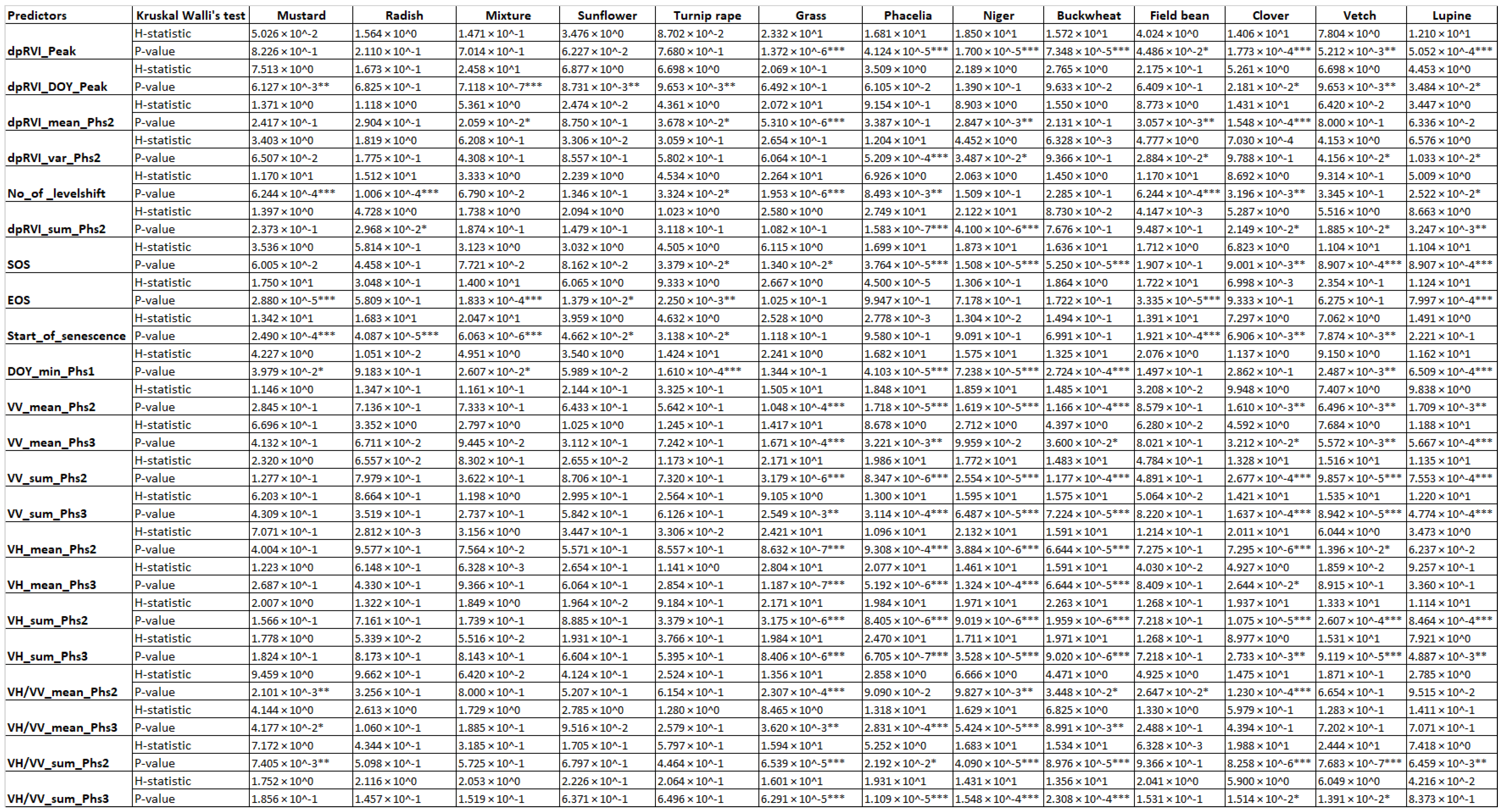
3.7. Kruskal–Wallis H-Test and Its Significance

Here, we conducted the Kruskal–Wallis test to assess the statistical differences among the extracted parameters for each catch crop, and the findings are summarized in Appendix A, Figure A1. The results indicate significant differences in most of the parameters across various catch crops. Particularly, most predictors exhibited high levels of significance for cold-sensitive varieties (phacelia, niger, and buckwheat), legume catch crops (clover, lupine, and vetch), and grass. The high H-statistics, coupled with a high level of significance at 0.001, suggests that these parameters are highly variable and, hence, can be viable inputs for distinguishing the abovementioned crops from other catch crops. This also helps to utilize crop-specific predictors for differentiating specific catch crop from other catch crop types.
Moreover, we groped all the catch crops into three groups (cold-tolerant, cold-sensitive, and legumes) as mentioned earlier, and conducted a Kruskal–Wallis test among these groups. The results are indicated in Table 4.
For instance, significant predictors such as dpRVI_Peak, SOS, VH_sum_Phs2 and Phs3, VV_sum_Phs2 and Phs3 and VV,VH_mean_Phs2 show particularly high H-values, suggesting strong distinctions among groups for these variables. The low p-values (p < 0.001, denoted as 0.000 ***) across most predictors except EOS (End_of_ Season) confirm the statistical significance, implying that the differences could be further utilized in the classification of catch crop types. To verify which catch crop groups are significantly different, we conducted pairwise Dunn’s test.

3.8. Dunn’s Post Hoc Test and Pairwise Significance

Here, we conducted the Dunn’s post hoc test for parameters that were found to be highly significant in the Kruskal–Wallis test, and the results are given in Table 5. The aim of Dunn’s test is to perform pairwise comparisons between groups to determine which specific groups differ from each other.
In Dunn’s test, the predictors such as VH_sum_Phs2, VH_sum_Phs3, VV_sum_Phs2, and VV_sum_Phs2 demonstrated high levels of significance across all pairs (CT/CS, CS/L, and L/CT). SOS shows high significance among CT/CS and CS/L and moderate sensitivity towards L/CT. The predictor dpRVI_Peak exhibited significant differences among CT/CS and CS/L group pairs (p < 0.001 ***). However, no significant difference was observed for the L/CT group pair. Similar results were seen with other predictors, such as VH_mean_Phs3, VH/VV_mean_Phs3, VH/VV_sum_Phs2, and VH/VV_sum_Phs3. On the other hand, dpRVI_DOY_Peak showed significant differences between CS/L (p < 0.001 ***) and L/CT (p = 0.003 **), highlighting variations in the day of the year between these crop groups. No significant differences were observed for the CT/CS pair in dpRVI_DOY_Peak. Predictors such as dpRVI_mean_Phs2, dpRVI_var_Phs2 do not show any significant differences across any crop pairs. These results from Dunn’s test not only confirm the significant predictors identified in the Kruskal–Wallis test but also clarify how these predictors vary between specific catch crop group pairs.

4. Discussion

The main aim of this study was to highlights the value of Sentinel-1 dense time series data and its important radar parameters to study the unique temporal characteristics of different catch crop groups in comparison to main crops. This discussion synthesizes the key findings and future research.
Radar parameters such as VV, VH, and VH/VV backscatter, dpRVI, and coherence were analyzed along with precipitation, temperature records, and ground-truth data. A notable signature difference was observed among different catch crop types based on their structure, phenological development, sowing time, temperature sensitiveness, and harvest timings, which, in turn, was fairly reflected in the Sentinel-1 temporal profiles. The type of main crop cultivated and their harvest have a great influence on the type and time of catch crop cultivation. This is based on our observation that winter wheat and winter barley, as dominant pre-crops, impact the sowing dates and growth patterns of subsequent catch crops. For instance, cold-sensitive varieties are typically sown earlier following the harvest of WB, which is harvested earlier than WW, allowing these crops to develop more biomass before winter (refer to SOS and DOY_min_Phs1 from Figure 14). Hence, the inclusion of the main crop in the temporal profile analysis gives the knowledge about the status quo, that is, the current crop rotations including catch crops [69,70].
A distinct temporal profile difference was observed between main crops and catch crops types (Section 3.1). We observed a high sensitivity of VV and VH backscatter to phenological stages and crop structure, which is especially evident in main crop cereals (WW and WB) during booting and heading stages. Both VV and VH backscatter decreases during the booting stage for both the cereals due to observed maximum signal attenuation. This is, again, followed by an increase in backscatter during the heading stage due to emerging vertical ear heads. This decrease and increase was observed recurrently in main crops for both the years. This pattern in cereals was also confirmed and reported by earlier studies [30,59,68]. Another interesting thing to note in VV and VH backscatter is their potential to indicate particular phenological events, such as the bending of ear heads in WB. During the heading stage of WB, the significant increase in backscatter values was observed in WB due to the bending of ear heads from vertical to horizontal orientation, causing a distinct pattern in the radar signal [30,71]. This phenomenon was not observed in profiles of winter wheat, which shows how SAR is sensitive to crop structural changes and useful in characterizing the short-term phenological events. Interestingly, this phenomena was not captured in the temporal profiles of VH/VV and dpRVI, as these parameters are not sensitive to crop structural changes [59].
Among catch crops, sunflower exhibited higher backscatter due to its broad leaf nature. Alternatively, grass has low backscatter due to its vertical structure, which leads to high signal attenuation, and this coincides with previous findings [72]. While there were some backscatter difference observed for catch crops during early stages and after, all the crops followed the same pattern, and profiles were found to be mixing with each other. Among legumes, clover and lupine had less backscatter, as expected, due to their less competitive nature and vigor. After December, interestingly, VV backscatter for green mixture started to increase in both years. Green mixtures often have a higher ratio of seed mixes that can grow in cold temperatures. Therefore, this increase in VV and VH can be attributed to the sprouting and growth of other cold-tolerant species during winter.
This study found that VH/VV and dpRVI were highly sensitive to biomass and vigor (Section 3.3), which was in accordance with the earlier findings [59,73]. Both the parameters increased with crop growth, reached maximum during peak vegetative phase, and again started to decreases. Interestingly, in both parameters, a slight decrease was observed during the heading stage. This may be due to the complex canopy architecture of cereals characterized by vertical ear heads that results in a high degree of randomness and multiple scattering effects in the heading stage, as reported by [55]. Our findings shows that VH/VV decreases a little early for cold-sensitive varieties and this can be attributed to their early die-off nature or due to some management activities carried out in the fields. In the case of legumes, a marked decline in backscatter was noted for lupine and clover at the onset of December. Given the high sensitivity of VH/VV backscatter to various management practices indicated in previous studies [59], this decrease could be due to activities such as mowing or other related management practices. Towards the end of February, VH/VV exhibits a noticeable rise, independent of specific crop varieties. This may be attributed to spontaneous vegetation growth following the removal of catch crops or the resurgence of previously sown seeds. Therefore, our study reconfirms that VH/VV could serve as a significant factor in assessing the post-harvest events. Compared to main crops, the dpRVI values are relatively lower for catch crops. This difference arises because catch crops often lack the intensive cultivation practices applied to main crops and are typically grown in autumn, which limits their full growth potential. Hence, the radar-based Vegetation Index acts as a robust indicator of crop health and growth dynamics, as reported in previous studies [74,75]. In general, the sensitivity of VH/VV and dpRVI to biomass underscores their potential in estimating crop yield and assessing crop health, which are critical for food security.
Interferometric coherence follows an opposite pattern compared to SAR backscatter and Vegetation Index concerning the crop growth cycle. Our findings revealed that coherence values are lower (ranging between 0.2 to 0.3) during the peak crop growing period for both main and catch crops. This phenomenon is primarily attributed to the high volume scattering from the crop canopy, resulting in a complete decorrelation of the phase, as reported by previous studies [58,76]. A slight increase in coherence values was observed for main crops as they approached the ripening and harvest stages, due to low-volume contributions from the crop fields. Interestingly, for catch crops, the coherence values started to increase from November for cold-sensitive varieties and from December for cold-tolerant and legume varieties. This increase in coherence values indicates a cessation of further growth or development in catch crops due to low temperatures, effectively marking the onset of the dormant phase that persists throughout the winter. A significant correlation was observed between different phenological stages (sowing, growth, and harvesting phase) of the crops and radar coherence, as observed by previous studies [77]. Hence, SAR coherence is found to be an important parameter for identifying broad phenological stages of catch crops such as the period of active crop growth, structural changes, and also to obtain an idea about the management practices. However, the high amount of noise present in coherence data, combined with the observed complete decorrelation during the crop growing phase, poses a significant challenge in using the coherence data for descriptive feature extraction. Given that SAR coherence exhibits higher sensitivity to moisture and precipitation [78], this aspect will be further investigated in the upcoming study.
The observed strong positive trend in VV, VH, VH/VV and dpRVI parameters during early Autumn (starting from from August) for catch crops is promising and this can be factor to distinguish catch crops from winter main crops. This similar positive trend was reported in optical time series for catch crops [19]. Additionally, the observed wide sowing date difference between the main and catch crops combined with temporal pattern differences observed in radar signals further aids in distinguishing catch crops from winter main crops.
For this study, a total of 22 extracted descriptors and phenological metrics were extracted using an automated and robust phenological procedure from backscatter (VV, VH, VH/VV) and dpRVI for catch crops (Section 3.6) to serve as critical information sources for discriminating different catch crop types. In general, phenological metrics are commonly extracted using optical data. However, effective retrieval can be hindered by significant cloud cover throughout most of the winter period, leading to missing information. In contrast, microwave backscatter retrieval is practically unaffected by atmospheric conditions, allowing it to provide insights about how sowing, peak vegetative stage, and harvest timing vary with crop types, as reported in several studies [61]. Thus, this study investigated the potential of SAR data in general and S-1 data in particular to monitor the phenology of catch crops using previously automated and robust phenological procedures evaluated in many studies in the optical domain to separate the phenological cycles and estimate the phenological parameters from the time series [62,64].
The individual crop-wise H-test results showed that defined predictors based on dpRVI, VV, VH, and VH/VV have high statistical significance among different catch crop types, especially for cold-sensitive catch crops (phacelia, niger, and buckwheat), grass, clover, lupine, and vetch. This separability is primarily attributed to the early sowing of cold-sensitive varieties compared to others, which is reflected in the predictors, namely, Start_of_ Season (SOS), dpRVI_Peak, and dpRVI_DOY_Peak. This early sowing leads to accelerated biomass development, significantly influencing the SAR parameters. Due to the observed low biomass and less competitive growth characteristics, crops such as clover, lupine, and vetch demonstrate some degree of separability from other species. However, some catch crop types, such as mustard, radish, sunflower, turnip rape, and field bean, exhibit similar behavior and do not show significant differences in the Kruskal–Wallis test. Their planophile crop architecture, along with comparable growth patterns and tendencies [79], makes it challenging to distinguish. Promising results were obtained when catch crops were grouped into three broad categories. Dunn’s post hoc test revealed significant variations among cold-sensitive, cold-tolerant, and legume crops, providing a robust statistical foundation for further classification of catch crops. These advantageous additions, combined with the consistent temporal resolution of radar indices profiles across seasons, irrespective of environmental factors like cloud cover, further enhance the transferability of the phenological procedure. Additionally, the predictable annual growth pattern of catch crops during each growing season—such as being sown after the main crop harvest and harvested before the next planting season—ensures that the adopted approach for descriptors and phenological metrics retrieval remain robust and adaptable across various regions and timeframes, which adds to its overall effectiveness.
Our literature review states that no previous studies have focused on analyzing the detailed temporal behavior of catch crops using radar parameters. Therefore, this study acts as a reference and provides initial insights for future research employing SAR data to explore catch crop behavior. The current limitation of the study includes the reduced temporal resolution of time series from the year 2022, caused by the malfunctioning of the Sentinel-1 B sensor. However, this issue is expected to be resolved with the upcoming launch of Sentinel-1 C into orbit. While our study focuses exclusively on using data from the ascending orbit, it would be also interesting to combine and examine the data from the descending orbit to see the differences.

5. Conclusions

Since SAR has biggest advantage of obtaining continuous data both temporally and spatially, the information obtained from Sentinel-1 is highly reliable compared to optical data. Specifically for catch crops, where their entire growing period falls in the late autumn and winter months, developing an SAR-alone approach for catch crop mapping is essential. As a further step, studying Sentinel-1-based polarimetric parameters and their underlying scattering mechanism with respect to catch crop types is advantageous, which will be taken up in our upcoming study. With all the Sentinel-1-based potential parameters and the machine learning model, an effective approach can be developed for discriminating and mapping different catch crop types. The present study is limited to specific geographic region (Brunswick), which may affect the generalizability of the findings. To overcome this, reference data should be included across the whole of Germany. Additionally, including precise time series in situ data containing information about sowing, harvest, tillage, and plowing events combined with environmental variables can greatly contribute to robust models.

Author Contributions

Conceptualization, S.S., D.B. and H.G.; methodology, S.S., D.B., A.H. and H.G.; software, S.S. and A.H.; validation, S.S.; formal analysis, S.S.; investigation, S.S.; data curation, S.S.; writing—original draft preparation, S.S.; writing—review and editing, A.H., D.B. and H.G.; visualization, S.S.; supervision, D.B. and H.G.; project administration, H.G.; funding acquisition, H.G. All authors have read and agreed to the published version of the manuscript.

Funding

The project “KlimaFFolgen” is funded by the Federal Ministry of Food and Agriculture as part of the German Climate Protection Programme 2022.

Data Availability Statement

The codes and the datasets generated are available from the corresponding author upon request.

Acknowledgments

We thank our technical staff of the Research Center for Agricultural Remote Sensing (FLF) for their significant support in sampling and preparing ground truth data. We also thank the German Meteorological Service (DWD) for providing daily meteorological data. Lastly, we thank the operators of CODE-DE for providing a tailored EO cloud computing platform for public organisations.

Conflicts of Interest

The authors declare no conflicts of interest.

Appendix A. Kruskal-Wallis Crop-Wise Test Results

Figure A1. Kruskal Wallis H and p-value statistics for each predictor based on individual crop-wise test. *, **, *** indicate 0.05, 0.01, and 0.001 level of significance.
Remotesensing 16 03737 g0a1

References

  1. European Commission. Communication from the Commission to the European Parliament, the Council, the European Economic and Social Committee and the Committee of the Regions. Stepping up Europe’s 2030 Climate Ambition. Investing in a Climate-Neutral Future for the Benefit of Our People. Brussels, Belgium. 2020. Available online: https://eur-lex.europa.eu/legal-content/EN/TXT/PDF/?uri=CELEX:52020DC0562&from=en (accessed on 10 June 2024).
  2. Yıldız, T. Green Horizons: Reflections of the European Union’s Environmental Policy in Action. Int. J. Soc. Humanit. Sci. Res. (JSHSR) 2024, 11, 729–739. [Google Scholar]
  3. Blandford, D.; Hassapoyannes, K. The common agricultural policy in 2020: Responding to climate change. In Research Handbook on EU Agriculture Law; Edward Elgar Publishing: Northampton, MA, USA, 2015; pp. 170–202. [Google Scholar]
  4. De Castro, P.; Miglietta, P.P.; Vecchio, Y. The Common Agricultural Policy 2021–2027: A new history for European agriculture. Riv. Econ. Agrar. 2020, 75, 5–12. [Google Scholar]
  5. Blanco, H. Cover Crops and Soil Ecosystem Services; John Wiley & Sons, Inc.: Hoboken, NJ, USA, 2023; pp. 1–242. [Google Scholar] [CrossRef]
  6. Schipanski, M.E.; Barbercheck, M.; Douglas, M.R.; Finney, D.M.; Haider, K.; Kaye, J.P.; Kemanian, A.R.; Mortensen, D.A.; Ryan, M.R.; Tooker, J.; et al. A framework for evaluating ecosystem services provided by cover crops in agroecosystems. Agric. Syst. 2014, 125, 12–22. [Google Scholar] [CrossRef]
  7. Udupa, S.M. Project Final Report: Optimising Subsidiary Crop Applications in Rotations (OSCAR); European Union: Brussels, Belgium, 2016. [Google Scholar]
  8. Seitz, D.; Fischer, L.M.; Dechow, R.; Wiesmeier, M.; Don, A. The potential of cover crops to increase soil organic carbon storage in German croplands. Plant Soil 2023, 488, 157–173. [Google Scholar] [CrossRef]
  9. Delgado, J.A.; Dillon, M.A.; Sparks, R.T.; Essah, S.Y. A decade of advances in cover crops. J. Soil Water Conserv. 2007, 62, 110A–117A. [Google Scholar]
  10. KC, K.; Zhao, K.; Romanko, M.; Khanal, S. Assessment of the spatial and temporal patterns of cover crops using remote sensing. Remote Sens. 2021, 13, 2689. [Google Scholar] [CrossRef]
  11. Saad El Imanni, H.; El Harti, A.; Panimboza, J. Investigating Sentinel-1 and Sentinel-2 Data Efficiency in Studying the Temporal Behavior of Wheat Phenological Stages Using Google Earth Engine. Agriculture 2022, 12, 1605. [Google Scholar] [CrossRef]
  12. Brisco, B.; Brown, R.; Hirose, T.; McNairn, H.; Staenz, K. Precision agriculture and the role of remote sensing: A review. Can. J. Remote Sens. 1998, 24, 315–327. [Google Scholar] [CrossRef]
  13. Bargiel, D. A new method for crop classification combining time series of radar images and crop phenology information. Remote Sens. Environ. 2017, 198, 369–383. [Google Scholar] [CrossRef]
  14. Asam, S.; Gessner, U.; Almengor González, R.; Wenzl, M.; Kriese, J.; Kuenzer, C. Mapping crop types of Germany by combining temporal statistical metrics of Sentinel-1 and Sentinel-2 time series with LPIS data. Remote Sens. 2022, 14, 2981. [Google Scholar] [CrossRef]
  15. Steinhausen, M.J.; Wagner, P.D.; Narasimhan, B.; Waske, B. Combining Sentinel-1 and Sentinel-2 data for improved land use and land cover mapping of monsoon regions. Int. J. Appl. Earth Obs. Geoinf. 2018, 73, 595–604. [Google Scholar] [CrossRef]
  16. Blickensdörfer, L.; Schwieder, M.; Pflugmacher, D.; Nendel, C.; Erasmi, S.; Hostert, P. Mapping of crop types and crop sequences with combined time series of Sentinel-1, Sentinel-2 and Landsat 8 data for Germany. Remote Sens. Environ. 2022, 269, 112831. [Google Scholar] [CrossRef]
  17. Zhou, X.; Wang, J.; He, Y.; Shan, B. Crop classification and representative crop rotation identifying using statistical features of time-series sentinel-1 GRD data. Remote Sens. 2022, 14, 5116. [Google Scholar] [CrossRef]
  18. Ren, T.; Xu, H.; Cai, X.; Yu, S.; Qi, J. Smallholder crop type mapping and rotation monitoring in mountainous areas with Sentinel-1/2 imagery. Remote Sens. 2022, 14, 566. [Google Scholar] [CrossRef]
  19. Schulz, C.; Holtgrave, A.K.; Kleinschmit, B. Large-scale winter catch crop monitoring with sentinel-2 time series and machine learning–an alternative to on-site controls? Comput. Electron. Agric. 2021, 186, 106173. [Google Scholar] [CrossRef]
  20. Ahmed, Z.; Nalley, L.; Brye, K.; Green, V.S.; Popp, M.; Shew, A.M.; Connor, L. Winter-time cover crop identification: A remote sensing-based methodological framework for new and rapid data generation. Int. J. Appl. Earth Obs. Geoinf. 2023, 125, 103564. [Google Scholar] [CrossRef]
  21. Barnes, M.L.; Yoder, L.; Khodaee, M. Detecting winter cover crops and crop residues in the midwest US using machine learning classification of thermal and optical imagery. Remote Sens. 2021, 13, 1998. [Google Scholar] [CrossRef]
  22. Swoish, M.; Leme Filho, J.F.D.C.; Reiter, M.S.; Campbell, J.B.; Thomason, W.E. Comparing satellites and vegetation indices for cover crop biomass estimation. Comput. Electron. Agric. 2022, 196, 106900. [Google Scholar] [CrossRef]
  23. Prabhakara, K.; Hively, W.D.; McCarty, G.W. Evaluating the relationship between biomass, percent groundcover and remote sensing indices across six winter cover crop fields in Maryland, United States. Int. J. Appl. Earth Obs. Geoinf. 2015, 39, 88–102. [Google Scholar] [CrossRef]
  24. Roth, L.; Streit, B. Predicting cover crop biomass by lightweight UAS-based RGB and NIR photography: An applied photogrammetric approach. Precis. Agric. 2018, 19, 93–114. [Google Scholar] [CrossRef]
  25. Assmann, J.J.; Kerby, J.T.; Cunliffe, A.M.; Myers-Smith, I.H. Vegetation monitoring using multispectral sensors—Best practices and lessons learned from high latitudes. J. Unmanned Veh. Syst. 2018, 7, 54–75. [Google Scholar] [CrossRef]
  26. McNairn, H.; Shang, J.; Jiao, X.; Champagne, C. The contribution of ALOS PALSAR multipolarization and polarimetric data to crop classification. IEEE Trans. Geosci. Remote Sens. 2009, 47, 3981–3992. [Google Scholar] [CrossRef]
  27. Fieuzal, R.; Baup, F.; Marais-Sicre, C. Sensitivity of TerraSAR-X, RADARSAT-2 and ALOS satellite radar data to crop variables. In Proceedings of the 2012 IEEE International Geoscience and Remote Sensing Symposium, Munich, Germany, 22–27 July 2012; pp. 3740–3743. [Google Scholar] [CrossRef]
  28. Lopez-Sanchez, J.M.; Cloude, S.R.; Ballester-Berman, J.D. Rice Phenology Monitoring by Means of SAR Polarimetry at X-Band. IEEE Trans. Geosci. Remote Sens. 2012, 50, 2695–2709. [Google Scholar] [CrossRef]
  29. Shao, Y.; Fan, X.; Liu, H.; Xiao, J.; Ross, S.; Brisco, B.; Brown, R.; Staples, G. Rice monitoring and production estimation using multitemporal RADARSAT. Remote Sens. Environ. 2001, 76, 310–325. [Google Scholar] [CrossRef]
  30. Harfenmeister, K.; Spengler, D.; Weltzien, C. Analyzing temporal and spatial characteristics of crop parameters using Sentinel-1 backscatter data. Remote Sens. 2019, 11, 1569. [Google Scholar] [CrossRef]
  31. Tan, C.P.; Ewe, H.T.; Chuah, H.T. Agricultural crop-type classification of multi-polarization SAR images using a hybrid entropy decomposition and support vector machine technique. Int. J. Remote Sens. 2011, 32, 7057–7071. [Google Scholar] [CrossRef]
  32. Wang, D.; Lin, H.; Chen, J.; Zhang, Y.; Zeng, Q. Application of multi-temporal ENVISAT ASAR data to agricultural area mapping in the Pearl River Delta. Int. J. Remote Sens. 2010, 31, 1555–1572. [Google Scholar] [CrossRef]
  33. Shanmugapriya, S.; Haldar, D.; Danodia, A. Optimal datasets suitability for pearl millet (Bajra) discrimination using multiparametric SAR data. Geocarto Int. 2020, 35, 1814–1831. [Google Scholar] [CrossRef]
  34. Arias, M.; Campo-Bescós, M.Á.; Álvarez-Mozos, J. Crop classification based on temporal signatures of Sentinel-1 observations over Navarre province, Spain. Remote Sens. 2020, 12, 278. [Google Scholar] [CrossRef]
  35. Choudhury, I.; Chakraborty, M. SAR signature investigation of rice crop using RADARSAT data. Int. J. Remote Sens. 2006, 27, 519–534. [Google Scholar] [CrossRef]
  36. Sah, S.; Haldar, D.; Chandra, S.; Nain, A.S. Discrimination and monitoring of rice cultural types using dense time series of Sentinel-1 SAR data. Ecol. Inform. 2023, 76, 102136. [Google Scholar] [CrossRef]
  37. Betbeder, J.; Fieuzal, R.; Philippets, Y.; Ferro-Famil, L.; Baup, F. Contribution of multitemporal polarimetric synthetic aperture radar data for monitoring winter wheat and rapeseed crops. J. Appl. Remote Sens. 2016, 10, 026020. [Google Scholar] [CrossRef]
  38. Regional State of Play Analyses; Braunschweig, Germany. 2021. Available online: https://suwanu-europe.eu/wp-content/uploads/2021/05/State-of-play_Braunschweig-Germany.pdf (accessed on 12 July 2024).
  39. Regionalstatistik. Flächennutzung. Available online: https://www.regionalstatistik.de/genesis/online (accessed on 12 July 2024).
  40. Lüker-Jans, N.; Simmering, D.; Otte, A. Analysing data of the integrated administration and control system (IACS) to detect patterns of agricultural land-use change at municipality level. Landsc. Online 2016, 48. [Google Scholar] [CrossRef]
  41. Stein, S.; Steinmann, H.H. Identifying crop rotation practice by the typification of crop sequence patterns for arable farming systems—A case study from Central Europe. Eur. J. Agron. 2018, 92, 30–40. [Google Scholar] [CrossRef]
  42. Benz, U.; Banovsky, I.; Cesarz, A.; Schmidt, M. CODE-DE Portal Handbook; Version 2.0. 2020. Available online: https://code-de.cdn.prismic.io/code-de/ff151913-16e0-4dc3-8005-696bf25bf65d_User+Manual_v2.0.2_ENG.pdf (accessed on 15 March 2023).
  43. Srivastava, H.S.; Patel, P.; Prasad, S.; Sharma, Y.; Khan, B.A.; Praveen, B.; Sharma, S.; Vijayan, L.; Vijayan, V. Potential applications of multi-parametric synthetic aperture radar (SAR) data in wetland inventory: A case study of Keoladeo National Park (A World Heritage and Ramsar site), Bharatpur, India. In Proceedings of the 12th World Lake Conference, TAAL, Jaipur, India, 28 October–2 November 2007. [Google Scholar]
  44. Wood, D.; McNairn, H.; Brown, R.; Dixon, R. The effect of dew on the use of RADARSAT-1 for crop monitoring: Choosing Between Ascending and Descending Orbits. Remote Sens. Environ. 2002, 80, 241–247. [Google Scholar] [CrossRef]
  45. Khabbazan, S.; Vermunt, P.; Steele-Dunne, S.; Ratering Arntz, L.; Marinetti, C.; van der Valk, D.; Iannini, L.; Molijn, R.; Westerdijk, K.; van der Sande, C. Crop monitoring using Sentinel-1 data: A case study from The Netherlands. Remote Sens. 2019, 11, 1887. [Google Scholar] [CrossRef]
  46. Bouvet, A.; Le Toan, T.; Lam-Dao, N. Monitoring of the rice cropping system in the Mekong Delta using ENVISAT/ASAR dual polarization data. IEEE Trans. Geosci. Remote Sens. 2009, 47, 517–526. [Google Scholar] [CrossRef]
  47. McNairn, H.; Shang, J. A review of multitemporal synthetic aperture radar (SAR) for crop monitoring. In Multitemporal Remote Sensing: Methods and Applications; Springer: Cham, Switzerland, 2016; pp. 317–340. [Google Scholar]
  48. Chauhan, S.; Darvishzadeh, R.; Lu, Y.; Boschetti, M.; Nelson, A. Understanding wheat lodging using multi-temporal Sentinel-1 and Sentinel-2 data. Remote Sens. Environ. 2020, 243, 111804. [Google Scholar] [CrossRef]
  49. Blaes, X.; Vanhalle, L.; Defourny, P. Efficiency of crop identification based on optical and SAR image time series. Remote Sens. Environ. 2005, 96, 352–365. [Google Scholar] [CrossRef]
  50. DWD Climate Data Center (CDC). Available online: https://www.dwd.de/EN/climate_environment/cdc/ (accessed on 17 September 2024).
  51. Baumann, P. A general conceptual framework for multi-dimensional spatio-temporal data sets. Environ. Model. Softw. 2021, 143, 105096. [Google Scholar] [CrossRef]
  52. McClelland, J.; Riedel, T.; Beyer, F.; Gerighausen, H.; Golla, B. State of the Art Open Access Remote Sensing with ESA Sentinel 1 SAR Data; Gesellschaft für Informatik e.V.: Bonn, Germany, 2023. [Google Scholar]
  53. Truckenbrodt, J.; Cremer, F.; Baris, I.; Eberle, J. pyroSAR—A Framework for Large-Scale SAR Satellite Data Processing. In Proceedings of the Big Data from Space, Munich, Germany, 19–21 February 2019; pp. 19–20. [Google Scholar]
  54. Guo, Z.; Qi, W.; Huang, Y.; Zhao, J.; Yang, H.; Koo, V.C.; Li, N. Identification of crop type based on C-AENN using time series Sentinel-1A SAR data. Remote Sens. 2022, 14, 1379. [Google Scholar] [CrossRef]
  55. Mandal, D.; Kumar, V.; Ratha, D.; Dey, S.; Bhattacharya, A.; Lopez-Sanchez, J.M.; McNairn, H.; Rao, Y.S. Dual polarimetric radar vegetation index for crop growth monitoring using sentinel-1 SAR data. Remote Sens. Environ. 2020, 247, 111954. [Google Scholar] [CrossRef]
  56. Mandal, D.; Bhattacharya, A.; Rao, Y.S.; Mandal, D.; Bhattacharya, A.; Rao, Y.S. Radar vegetation indices for crop growth monitoring. In Radar Remote Sensing for Crop Biophysical Parameter Estimation; Springer: Singapore, 2021; pp. 177–228. [Google Scholar]
  57. Touzi, R.; Lopes, A.; Bruniquel, J.; Vachon, P.W. Coherence estimation for SAR imagery. IEEE Trans. Geosci. Remote Sens. 1999, 37, 135–149. [Google Scholar] [CrossRef]
  58. Amherdt, S.; Di Leo, N.C.; Pereira, A.; Cornero, C.; Pacino, M.C. Assessment of interferometric coherence contribution to corn and soybean mapping with Sentinel-1 data time series. Geocarto Int. 2022, 38, 1–22. [Google Scholar] [CrossRef]
  59. Veloso, A.; Mermoz, S.; Bouvet, A.; Le Toan, T.; Planells, M.; Dejoux, J.F.; Ceschia, E. Understanding the temporal behavior of crops using Sentinel-1 and Sentinel-2-like data for agricultural applications. Remote Sens. Environ. 2017, 199, 415–426. [Google Scholar] [CrossRef]
  60. Tamm, T.; Zalite, K.; Voormansik, K.; Talgre, L. Relating Sentinel-1 interferometric coherence to mowing events on grasslands. Remote Sens. 2016, 8, 802. [Google Scholar] [CrossRef]
  61. Meroni, M.; d’Andrimont, R.; Vrieling, A.; Fasbender, D.; Lemoine, G.; Rembold, F.; Seguini, L.; Verhegghen, A. Comparing land surface phenology of major European crops as derived from SAR and multispectral data of Sentinel-1 and-2. Remote Sens. Environ. 2021, 253, 112232. [Google Scholar] [CrossRef]
  62. Htitiou, A.; Möller, M.; Riedel, T.; Beyer, F.; Gerighausen, H. Towards Optimising the Derivation of Phenological Phases of Different Crop Types over Germany Using Satellite Image Time Series. Remote Sens. 2024, 16, 3183. [Google Scholar] [CrossRef]
  63. Haldar, D.; Verma, A.; Kumar, S.; Chauhan, P. Estimation of mustard and wheat phenology using multi-date Shannon entropy and Radar Vegetation Index from polarimetric Sentinel-1. Geocarto Int. 2022, 37, 5935–5962. [Google Scholar] [CrossRef]
  64. White, M.A.; Thornton, P.E.; Running, S.W. A continental phenology model for monitoring vegetation responses to interannual climatic variability. Glob. Biogeochem. Cycles 1997, 11, 217–234. [Google Scholar] [CrossRef]
  65. Kruskal, W.H.; Wallis, W.A. Use of ranks in one-criterion variance analysis. J. Am. Stat. Assoc. 1952, 47, 583–621. [Google Scholar] [CrossRef]
  66. Jett, D.; Speer, J. Comparison of parametric and nonparametric tests for differences in distribution. In Proceedings of the National Conference on Undergraduate Research (NCUR), Asheville, NC, USA, 7–9 April 2016; pp. 7–9. [Google Scholar]
  67. Pohlert, T. The pairwise multiple comparison of mean ranks package (PMCMR). R Package 2014, 27, 9. [Google Scholar]
  68. Xie, G.; Niculescu, S. Mapping crop types using sentinel-2 data machine learning and monitoring crop phenology with sentinel-1 backscatter time series in pays de Brest, Brittany, France. Remote Sens. 2022, 14, 4437. [Google Scholar] [CrossRef]
  69. Junod, M.F.; Reid, B.; Sims, I.; Miller, A.J. Cover crops in cereal rotations: A quantitative review. Soil Tillage Res. 2024, 238, 105997. [Google Scholar] [CrossRef]
  70. Nichols, G.A.; MacKenzie, C.A. Identifying research priorities through decision analysis: A case study for cover crops. Front. Sustain. Food Syst. 2023, 7, 1040927. [Google Scholar] [CrossRef]
  71. Domínguez Costa, A. Classification of Wheat and Barley Fields Using High-Resolution Sentinel-1 Backscatter Data. Bachelor’s Thesis, Universitat Politècnica de Catalunya, Barcelona, Spain, 2020. [Google Scholar]
  72. Nasirzadehdizaji, R.; Balik Sanli, F.; Abdikan, S.; Cakir, Z.; Sekertekin, A.; Ustuner, M. Sensitivity analysis of multi-temporal Sentinel-1 SAR parameters to crop height and canopy coverage. Appl. Sci. 2019, 9, 655. [Google Scholar] [CrossRef]
  73. Schuster, C.; Förster, M.; Kleinschmit, B. Testing the red edge channel for improving land-use classifications based on high-resolution multi-spectral satellite data. Int. J. Remote Sens. 2012, 33, 5583–5599. [Google Scholar] [CrossRef]
  74. Haldar, D.; Dave, V.; Misra, A.; Bhattacharya, B. Radar Vegetation Index for assessing cotton crop condition using RISAT-1 data. Geocarto Int. 2020, 35, 364–375. [Google Scholar] [CrossRef]
  75. Steele-Dunne, S.C.; McNairn, H.; Monsivais-Huertero, A.; Judge, J.; Liu, P.W.; Papathanassiou, K. Radar remote sensing of agricultural canopies: A review. IEEE J. Sel. Top. Appl. Earth Obs. Remote Sens. 2017, 10, 2249–2273. [Google Scholar] [CrossRef]
  76. Villarroya-Carpio, A.; Lopez-Sanchez, J.M.; Engdahl, M.E. Sentinel-1 interferometric coherence as a vegetation index for agriculture. Remote Sens. Environ. 2022, 280, 113208. [Google Scholar] [CrossRef]
  77. Nasirzadehdizaji, R.; Cakir, Z.; Sanli, F.B.; Abdikan, S.; Pepe, A.; Calo, F. Sentinel-1 interferometric coherence and backscattering analysis for crop monitoring. Comput. Electron. Agric. 2021, 185, 106118. [Google Scholar] [CrossRef]
  78. Barrett, B.; Whelan, P.; Dwyer, E. The use of C-and L-band repeat-pass interferometric SAR coherence for soil moisture change detection in vegetated areas. Open Remote Sens. J. 2012, 5, 37–53. [Google Scholar] [CrossRef]
  79. Haldar, D.; Chakraborty, M.; Manjunath, K.; Parihar, J. Role of polarimetric SAR data for discrimination/biophysical parameters of crops based on canopy architecture. Int. Arch. Photogramm. Remote Sens. Spat. Inf. Sci. 2014, 40, 737–744. [Google Scholar] [CrossRef]
Figure 1. Location of study area and sample points collected on five different dates during the year 2021 and 2022. The extents of Sentinel-1 relative orbits tiles 177 and 44 are shown in the location map.
Remotesensing 16 03737 g001
Figure 2. Some of the catch crop fields encountered during field survey: (a) mustard, (b) oilseed radish, (c) phacelia, (d) clover, (e) niger, and (f) green mixture.
Remotesensing 16 03737 g002
Figure 3. Phenological stages of different crops in the study area and corresponding Sentinel-1 data acquisitions in the years 2021 (blue) and 2022 (red).
Remotesensing 16 03737 g003
Figure 4. Example of a real mustard catch crop field where the entire profile of (a) VV backscatter, (b) VH backscatter, (c) VH/VV backscatter, and (d) dpRVI is divided into three phases based on detected peak and minimum values.
Remotesensing 16 03737 g004
Figure 5. Temporal VV backscatter profile of main crops followed by different catch crop categories: (a) cold-tolerant, (b) cold-sensitive, (c) legumes for the years 2021 (left) and 2022 (right). The vertical dashed lines (black color) indicate the harvest of the main crop.
Remotesensing 16 03737 g005
Figure 6. Temporal VH backscatter profile of main crops followed by different catch crop categories: (a) cold-tolerant, (b) cold-sensitive, (c) legumes for the years 2021 (left) and 2022 (right). The vertical dashed lines (black color) indicate the harvest of main crop.
Remotesensing 16 03737 g006
Figure 7. Temporal VH/VV backscatter profile of main crops followed by different catch crop categories: (a) cold-tolerant, (b) cold-sensitive, (c) legumes for the years 2021 (left) and 2022 (right). The vertical dashed lines (black color) indicate the harvest of main crop.
Remotesensing 16 03737 g007
Figure 8. Temporal dpRVI profile of main crops followed by different catch crop categories: (a) cold-tolerant, (b) cold-sensitive, (c) legumes for the years 2021 (left) and 2022 (right). The vertical dashed lines (black color) indicate the harvest of main crop.
Remotesensing 16 03737 g008
Figure 9. Temporal VV coherence profile of main crops followed by different catch crop categories: (a) cold-tolerant, (b) cold-sensitive, (c) legumes for the years 2021 (left) and 2022 (right). The vertical dashed lines (black color) indicate the harvest of main crop.
Remotesensing 16 03737 g009
Figure 10. Comparison of mean VV backscatter profiles: (a) winter oilseed rape, (b) winter cereals, (c) fallow/catch crop. The dashed lines (black) indicate the sowing time.
Remotesensing 16 03737 g010
Figure 11. Comparison of VH backscatter profiles: (a) winter oilseed rape, (b) winter cereals, (c) fallow/catch crop. The dashed lines (black) indicate the sowing time.
Remotesensing 16 03737 g011
Figure 12. Comparison of VH/VV backscatter profiles: (a) winter oilseed rape, (b) winter cereals, (c) fallow/catch crop. The dashed lines (black) indicate the sowing time.
Remotesensing 16 03737 g012
Figure 13. Comparison of dpRVI profiles: (a) oilseed rape, (b) winter cereals, (c) fallow/catch crop. The doted lines (black) indicate the sowing time.
Remotesensing 16 03737 g013
Figure 14. Box plot depicting the different predictors extracted from dpRVI time series for different catch crop types.
Remotesensing 16 03737 g014
Figure 15. Box plot depicting the different predictors extracted from VV, VH and VH/VV backscatter time series for different catch crop types.
Remotesensing 16 03737 g015
Table 1. Catch crop categories and number of samples collected per year for each crop type.
No.CategoriesCatch CropsNo. of Samples
20212022
1Cold tolerantMustard110117
Oilseed radish3628
Green mixture6665
Sunflower1311
Grass9-
Turnip rape-13
2Cold sensitivePhacelia2013
Niger139
Buckwheat6-
3LegumesField bean78
Lupine6-
Clover914
Vetch1111
Table 2. Sentinel-1 data specifications used in the study. Note that the temporal resolution is reduced to 12 days for the year 2022 due to the malfunctioning of the Sentinel-1B sensor.The incidence angle range given here is definite to the study area (Brunswick).
Sensor ParametersSpecifications
WavelengthC-band
Frequency5.405 GHz
Product typeGRD, SLC
Incidence angle37.4°–45.1°
Acquisition modeIW
Satellite passAscending (ASC)
Polarization modeVV, VH
Spatial resolution10 × 10 m
Temporal resolution6 days for 2021,
12 days for 2022
Table 3. Extracted descriptive features and their descriptions.
Descriptive FeatureDescriptionExample of Mustard Catch Crop Parcel
dpRVI_DOY_PeakThe day when the peak DpRVI value is reached and is computed by considering both Phase 2 and Phase 3. For cold-sensitive varieties and early-sown varieties, the DOY peak is expected to be early.
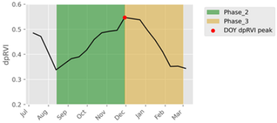
Remotesensing 16 03737 i001
dpRVI_PeakThe dpRVI value on the day of peak. The peak value is expected to change with type of catch crop and high/low biomass.Remotesensing 16 03737 i002
Start_of_Season (SOS)The day when dpRVI first reaches the 10% increase in seasonal amplitude of dpRVI from the minimum level in Phase 2, denoting the start of the growing phase of catch crops. For cold-sensitive varieties, SOS is expected to be early than other varieties due to their early sowing.
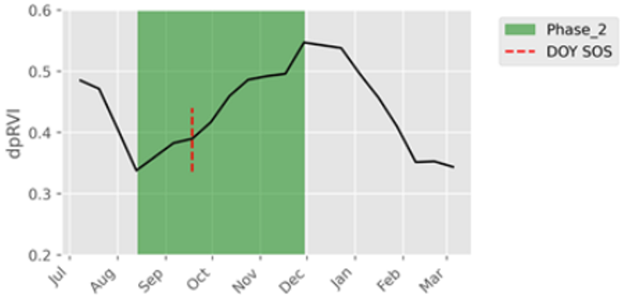
Remotesensing 16 03737 i003
End_of_Season (EOS)The day when dpRVI first reaches 10% decrease in seasonal amplitude of dpRVI from the minimum level in Phase 3, indicating the end of the growing season of catch crops. For cold-sensitive varieties, EOS is expected to be early than other varieties due to their early die-off nature.Remotesensing 16 03737 i004
Start_of_senescenceThe day when dpRVI first reaches 90% of the seasonal amplitude from the minimum level in Phase 3, indicating the onset of senescence of catch crops. The DOY of senescence varies according to the early harvest or die-off nature and frozen events of the catch crop classes.Remotesensing 16 03737 i005
DOY_min_Phs1The day when the first local minima of dpRVI is reached in Phase 1. This indicates the harvest of main crops (winter wheat or winter barley). Harvest dates are expected to be early for cold-sensitive ones and late for cold-tolerant varieties.Remotesensing 16 03737 i006
Number_of_levelshiftThe number of level-shift points, indicating the abrupt changes in the time series of dpRVI and calculated by taking into account of entire time period of Phase 1 and Phase 2. With harvest, plowing, mowing, frost, and precipitation events, the number of level shifts tends to increase.Remotesensing 16 03737 i007
DpRVI_var_Phs2This denotes the steadiness of vegetation activity temporally and is calculated by taking mean variance in Phase 2. The observed variance increases with management activities such as plowing, harvest and so on.Remotesensing 16 03737 i008
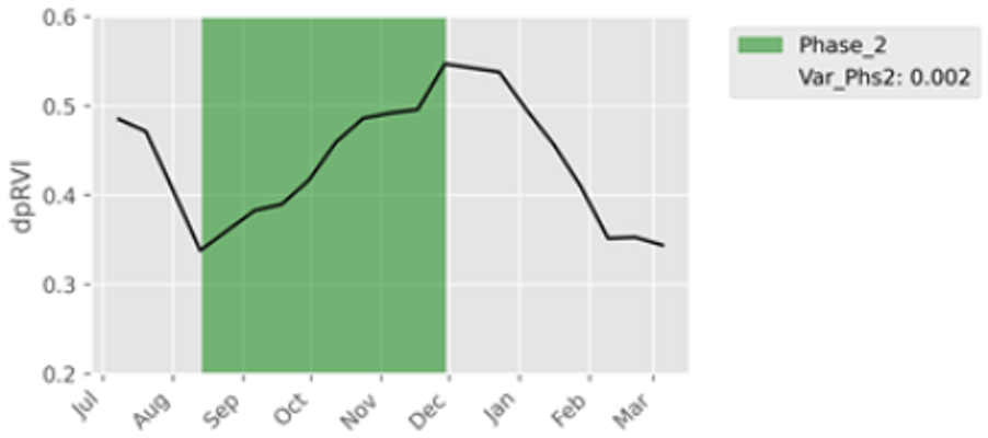
VV_Mean_Phs2, VH_Mean_Phs2, VH/VV_Mean_Phs2, dpRVI_Mean_Phs2This denotes the active vegetation cover of catch crop parcel and is computed by taking the mean of given parameter (VV, VH, VH/VV backscatter and dpRVI) in Phase 2 and high value indicates the successful catch crop cultivation.Remotesensing 16 03737 i009
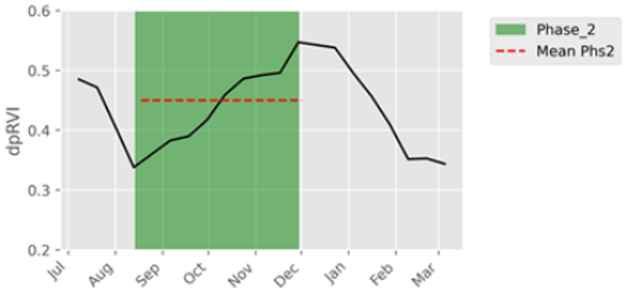
VV_Sum_Phs2, VH_Sum_Phs2, VH/VV_Sum_Phs2, dpRVI_Sum_Phs2This denotes the cumulative sum of given parameter (VV, VH, VH/VV backscatter and dpRVI) in Phase 2 and the values vary according to strength of vegetative cover of the catch crop field.Remotesensing 16 03737 i010
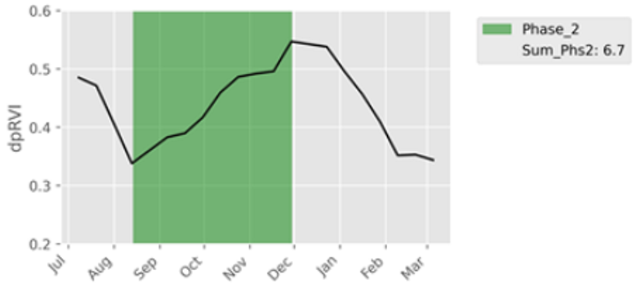
VV_Mean_Phs3, VH_Mean_Phs3, VH/VV_Mean_Phs3Computed by taking the mean of given parameter such as VV, VH, and VH/VV backscatter in Phase 3. The relatively observed low values (compared to Phase 1) correspond to loss of chlorophyll and vegetation water content (decrease in strength of vegetation activity) as the catch crop progresses towards ripening and harvest (note that dpRVI is excluded due to no significant difference).Remotesensing 16 03737 i011
VV_Sum_Phs3, VH_Sum_Phs3, VH/VV_Sum_Phs3Cumulative sum of VV, VH, VH/VV backscatter, respectively, of the given parcel in Phase 3. The relatively observed low sum values compared to Phase 1 indicate a decrease in the strength of vegetation as the crop enters the ripening and harvest phase (note dpRVI is excluded due to no significant difference).Remotesensing 16 03737 i012
Table 4. Kruskal –Wallis H and p-value statistics for each predictor conducted between three catch crop groups. **, *** given in the table indicate 0.01 and 0.001 level of significance.
No.PredictorsKruskal Wallis Test
H-Statisticp-Value
1dpRVI_Peak64.7910.000 ***
2dpRVI_DOY_Peak21.4940.000 ***
3dpRVI_mean_Phs211.0390.003 **
4dpRVI_var_Phs220.7760.000 ***
5No_of_levelshift20.1270.000 ***
6dpRVI_sum_Phs241.7880.000 ***
7SOS74.3620.000 ***
8EOS1.2160.544
9Start_of_senescence42.7720.000 ***
10DOY_min_Phs161.8220.000 ***
11VV_mean_Phs267.830.000 ***
12VV_mean_Phs331.4560.000 ***
13VV_sum_Phs273.1050.000 ***
14VV_sum_Phs371.2020.000 ***
15VH_mean_Phs264.2120.000 ***
16VH_mean_Phs361.9670.000 ***
17VH_sum_Phs286.4950.000 ***
18VH_sum_Phs379.3920.000 ***
19VH/VV_mean_Phs228.4040.000 ***
20VH/VV_mean_Phs350.0860.000 ***
21VH/VV_sum_Phs244.8790.000 ***
22VH/VV_sum_Phs356.7180.000 ***
Table 5. Dunn’s post hoc test results with Bonferroni correction for pairwise comparison among catch crop groups (CT refers to cold-tolerant, CS to cold-sensitive, and L refers legume catch crop groups) Note that the *, **, *** given indicate 0.05, 0.01 and 0.001 level of significance.
PredictorsCT/CSCS/LL/CT
dpRVI_Peak1.35 × 10 10 ***3.90 × 10 14 ***1.71 × 10 1
dpRVI_DOY_Peak2.57 × 10 1 2.60 × 10 6 ***2.17 × 10 3 **
dpRVI_mean_Phs21.27 × 10 2 *5.59 × 10 3 **1.000
dpRVI_var_Phs26.04 × 10 2 1.96 × 10 1 1.43 × 10 2 *
No_of_levelshift8.00 × 10 4 ***5.29 × 10 1 9.84 × 10 4 ***
dpRVI_sum_Phs25.11 × 10 6 ***1.08 × 10 3 **6.58 × 10 1
SOS3.29 × 10 9 ***3.34 × 10 17 ***1.66 × 10 3 **
Start_of_senescence2.02 × 10 2 *7.84 × 10 3 **1.96 × 10 10 ***
DOY_min_Phs19.06 × 10 9 ***1.34 × 10 3 **1.48 × 10 2 *
VV_mean_Phs23.00 × 10 10 ***3.54 × 10 15 ***1.60 × 10 5 ***
VV_mean_Phs32.84 × 10 2 *3.54 × 10 12 ***6.96 × 10 4 ***
VV_sum_Phs21.80 × 10 9 ***9.77 × 10 17 ***1.67 × 10 6 ***
VV_sum_Phs33.97 × 10 2 *1.91 × 10 14 ***1.49 × 10 4 ***
VH_mean_Phs21.51 × 10 9 ***1.009.08 × 10 1
VH_mean_Phs38.53 × 10 14 ***1.34 × 10 5 ***1.18 × 10 1
VH_sum_Phs24.12 × 10 13 ***1.36 × 10 11 ***2.34 × 10 4 ***
VH_sum_Phs32.98 × 10 12 ***1.18 × 10 10 ***1.67 × 10 5 ***
VH/VV_mean_Phs27.07 × 10 1 4.74 × 10 6 ***4.17 × 10 3 **
VH/VV_mean_Phs34.53 × 10 12 ***2.09 × 10 7 ***2.17 × 10 3 **
VH/VV_sum_Phs24.00 × 10 14 ***4.70 × 10 15 ***1.000
VH/VV_sum_Phs31.47 × 10 12 ***2.70 × 10 9 ***1.000
Disclaimer/Publisher’s Note: The statements, opinions and data contained in all publications are solely those of the individual author(s) and contributor(s) and not of MDPI and/or the editor(s). MDPI and/or the editor(s) disclaim responsibility for any injury to people or property resulting from any ideas, methods, instructions or products referred to in the content.

