Research on Digital Twin Method for Spaceborne Along-Track Interferometric Synthetic Aperture Radar Velocity Inversion of Ocean Surface Currents

Abstract

In this paper, an end-to-end system framework is proposed for the Digital Twin study of spaceborne ATI-SAR ocean current velocity inversion. Within this framework, a fitting inversion approach is proposed to enhance the conventional spaceborne ATI-SAR ocean current velocity inversion algorithm. Consequently, the issue of possible local inversion errors stemming from the mismatch between the traditional spaceborne ATI-SAR inversion algorithm and various dual-antenna configurations is resolved to a certain extent. A simulated spaceborne ATI-SAR system, featuring a dual-antenna configuration comprising a baseline direction perpendicular to the track and a squint angle, is presented to validate the efficacy of the Digital Twin methodology. Under the specified simulation parameters, the average inversion error for the final ocean current velocity is recorded at 0.0084 m/s, showcasing a reduction of 0.0401 m/s compared with the average inversion error prior to optimization.

1. Introduction

The ocean plays a crucial role in the Earth’s ecosystem, with its surface currents significantly influencing the transport of marine nutrients, global climate patterns, and human shipping activities [1]. As a result, the observation of ocean surface currents stands out as a prominent research focus within remote sensing technology. By monitoring and understanding these currents, scientists can gain valuable insights into various environmental processes and phenomena, contributing to a deeper comprehension of our planet’s interconnected systems and facilitating informed decision-making in areas such as marine resource management, climate studies, and human activities. Early current measurement methods mainly include the Lagrange method [2] and the Euler method [3]. The common feature of these two methods is that they infer the overall current information from local current information. Due to the limited detection range and harsh coastal environment, it is difficult to achieve real-time and overall monitoring. At present, synthetic aperture radar (SAR), with its all-time, all-weather, high resolution, and wide detection range [4], has become the mainstream technical method for monitoring ocean surface currents. By transmitting electromagnetic waves to the ocean surface, SAR receives and processes the echo signal, and extracts the amplitude and phase information, so as to realize the monitoring of ocean surface currents. In 1987, Goldstein and Zebker first proposed the along-track interferometric (ATI) SAR method [5], demonstrating that ocean surface currents can be inversed based on the Doppler effect, namely the frequency shift of a transmitted electromagnetic wave due to the relative movement between the transmitter and the ocean surface currents. The specific implementation method is that two antennas are placed in the moving track direction of the SAR platform to detect and image the same ocean surface. Due to the imaging delay, the velocity of the ocean surface currents will be manifested in the phase difference between the two echo signals. Since then, the potential of current measurements employing ATI-SAR has been explored in a number of studies. In terms of the airborne platform, in 1993, Thompson and Jensen [6] applied the ATI-SAR method to the data measured by the Jet Propulsion Laboratory of National Aeronautics and Space Administration (NASA) in California, United States and showed how the pixel-to-pixel phase difference is actually related to the mean Doppler frequency of the backscattered field. In 1996, Graber and Thompson [7] made the first quantitative comparison between high-resolution ocean surface current fields extracted from interferometric SAR (InSAR) and those from a high-frequency (HF) ocean surface current radar (OSCR), based on the measured data of the high-resolution remote sensing experiment (High-Res). The results indicate that high-resolution ocean surface current vectors can be derived from InSAR and the ATI-SAR method shows better performance on studying the dynamics of small-scale surface features in regions of strong current divergences or shears. In 2005, Romeiser [8] developed the ATI-SAR theory by proposing the algorithms for the inversion of two-dimensional surface current fields. Additionally, an effective numerical model suite M4S, which will be introduced in detail later in this paper, came into use to help remove the spatially varying contributions of surface wave motions on the same order of magnitude as the actual current field. Altogether, Romeiser made the ATI-SAR theory for current inversion more efficient, robust, and mature for applications. Also in 2005, Toporkov [9] proposed a dual-beam interferometry system, consisting of two interferometric synthetic aperture radars with different squint angles to allow measurements of currents with a single aircraft pass, further developing the ATI-SAR theory. In terms of the spaceborne platform, in 2007, the first satellite equipped with ATI mode emerged. Romeiser [10] presented the first analysis of the ocean surface current fields derived from the TerraSAR-X ATI-SAR data, where the phased-array SAR antenna is divided into two halves for receiving. In this case, the receiver is multiplexed to process two signals in an alternating way at a doubled pulse repetition frequency. The ATI performance of TerraSAR-X was observed to align closely with theoretical predictions. Other known satellites equipped with ATI mode mainly include SRTM-SAR, RadarSat-2, TANTANDEM X, and GF-3 satellites [11,12,13], and relevant satellite sensor research has been continuing.

In line with the task requirements, the configuration and system parameters of ATI-SAR on a satellite platform often vary, necessitating numerous simulation experiments for validation before task execution. Corresponding theoretical studies [14,15] have been conducted to figure out the mechanism of how the system parameters, such as radar frequency, along-track baseline, incident angle, etc., affect the quality of ATI data and what the most promising parameter combination for accurate ocean current inversion is. Based on the research above, it relies on the placement of dual antennas along the track to accurately determine the exact length of the along-track baseline, which has a significant influence on the inversion results of the ocean current field. Additionally, Romeiser pointed out that the ideal effective along-track baseline for spaceborne X-band ATI-SAR systems should be on the order of 20–30 m. A shorter one would cause a suboptimal sensitivity to scatter velocities and produce phase noise over thousands of full-resolution pixels where the processing of average filtering of the actually obtained interferometric phase is needed. In contrast, a longer one would also affect the data quality because of the temporal decorrelation of the backscattered signal [16]. However, most spaceborne ATI-SAR systems at present cannot achieve an ideal effective along-track baseline such as the SRTM-SAR [17] and TerraSAR-X [18,19], with only 3.5 m and 1 m, respectively. The performance of TanDEM-X was also affected in regions of improperly long along-track baseline [20]. The reason for this issue mainly lies in the multi-mode of the satellite which, as technology advances, may incorporate additional operational modes like altimetry and imaging alongside ATI-SAR functionality. In such cases, the antenna configuration may no longer be exclusively tailored for ATI-SAR velocity inversion and is called cross-track InSAR (XTI-SAR) [21]. It should be noted that this paper focuses on the velocity inversion of the ocean surface current instead of the height information, and the corresponding interferometric phase caused by the current scatter’s height would be eliminated before the velocity inversion, assuming that the scatter’s average height is known. Consequently, the effective along-track baseline may vary based on the specific observation geometry and the corresponding inversion algorithm needs to be adjusted. However, even with the time-consuming algorithm adjustment, fluctuating inversion errors still can arise. For example, the results of current field inversion of the TerraSAR-X [17] are consistent with the theoretical model in several cases, while unrealistic variations across the images are found in certain cases, which is confusing. Romeiser attributed it to shortcomings of the raw data processing algorithm. This is partially due to the systematic errors introduced by the mismatch between the actual observation geometry and the adjusted ATI-SAR algorithm, and partially due to the too-long or too-short effective along-track baseline, as mentioned before. In addition to radar parameters, ocean surface conditions such as shoaling waves [22] and internal waves [23] also affect the accuracy of current inversion. The former is the wave transmitted to the coast by the swell in the ocean and results in the deformation and enhancement of the ocean current in the shallow area. The latter would make the water particles move in the opposite direction at the interface, and the maximum velocity shear occurs at the interface, which can form an internal wave flow with a speed of up to 1.5 m/s. Both of them could affect the surface current in certain cases. Moreover, due to the necessity of reducing carbon emissions, many offshore wind turbines are being constructed and come into use widely, which may also contribute to the inversion error of surface currents because of their varying interference in the interferometric phase of SAR images [24]. Consequently, based on the analysis above, there is a need to find a method that strikes a balance between time efficiency and inversion accuracy when faced with the issue of a non-classical ATI-SAR antenna configuration with a non-ideal along-track baseline.

The concept of Digital Twin (DT) has emerged as a new idea in recent years. At its core, DT involves creating a virtual simulation system that mirrors the entire lifecycle of physical entities. By constructing high-fidelity physical models and enabling accurate mapping of real-world entities through data interaction, DT aims to replicate physical systems as closely as possible [25]. Given the intricate nature of radar-related physical systems, leveraging the Digital Twin concept and technology in the development and testing of radar systems can offer significant advantages and convenience in enhancing their functionality and performance. Since 2019, more and more researchers have begun to carry out relevant studies: T. Ruffetde et al. first proposed the concept of DT in radar simulation and showed us how to build a completely virtual radar system (VRS) [26]. A. V. Timoshenko et al. proposed a method of sequential development of DT of radar stations using a full-function model [27]. A. Karboski et al. proposed an AESA DT, which can model AESA and weather radar echoes and explore the optimal configuration of the APAR subsystem [28]. Xie et al. studied the implementation of DT in a UAV radar network and proposed a relevant UAV application framework [29].

Inspired by the research above, this paper proposes the application of the Digital Twin concept to the research of spaceborne ATI-SAR ocean surface current velocity inversion. The aim is to develop a comprehensive Digital Twin system framework for this purpose. As mentioned before, a non-classical dual-antenna configuration would cause an ambiguous effective along-track baseline, which may be shorter or longer than the ideal one based on the specific antenna configuration and the corresponding observation geometry, thus leading to inversion error resulting from both the non-ideal along-track baseline and the possible mismatch between the theoretical algorithm adjustment and the actual observation geometry. However, due to the ability of constructing high-fidelity physical models, the Digital Twin system framework for spaceborne ATI-SAR ocean surface current inversion proposed in this paper enables the antenna configuration, system parameters, and the ocean surface current model to be set based on any possible requirements, which offers the potential and convenience of designing and validating algorithms to solve the problem. The DT-based fitting inversion method, derived from the traditional ATI-SAR inversion algorithm, is proposed within the Digital Twin system framework. One key benefit of this approach is its adaptability to almost any dual-antenna configuration and system parameter. It offers the advantage of accommodating the inversion error caused by a non-ideal effective along-track baseline and the possible mismatch between the adjusted ATI-SAR algorithm and the actual observation geometry through obtaining a radial velocity-interferometric phase fitting curve. The essence of the method lies in optimizing the inversion errors associated with prominent anomalies by leveraging experimental data characterized by low inversion errors, thereby enhancing the accuracy and robustness of the inversion process. The specific principle will be described in detail in Section 2.3.

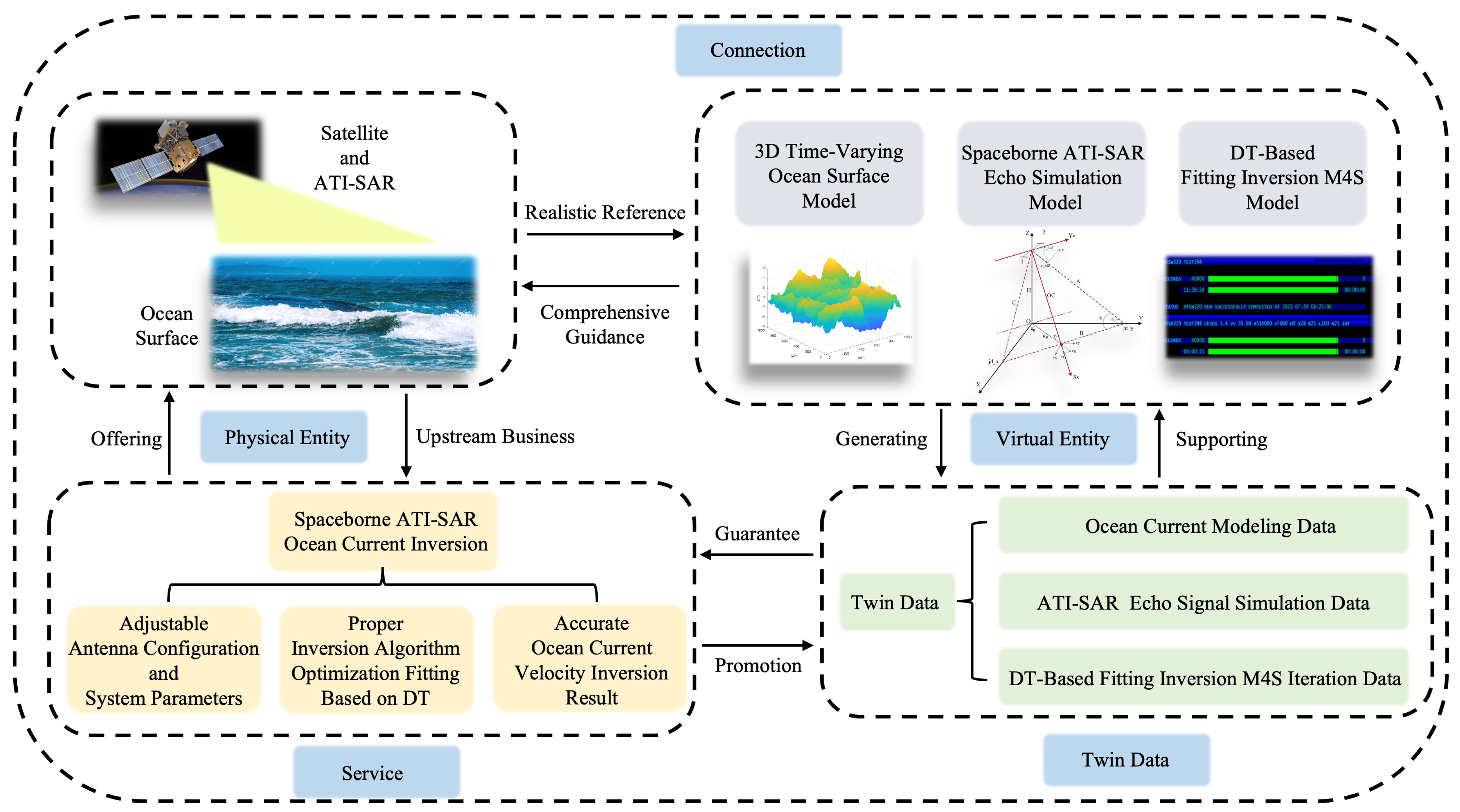
2. Construction of Digital Twin System for Spaceborne ATI-SAR Ocean Surface Current Inversion

Based on Professor Grieves’s three-dimensional Digital Twin model [30], Professor Tao Fei’s team introduced a five-dimensional Digital Twin model comprising the physical entity, virtual entity, service, twin data, and connection [25]. In accordance with this five-dimensional model theory, the end-to-end spaceborne ATI-SAR ocean surface current inversion Digital Twin system framework proposed in this study is illustrated in Figure 1, where each component interacts with the others. The physical entity shapes the basic structure of the virtual entity, which in turn analyzes twin data generated through algorithm iterations and offers decision support to the physical entity. If the service fails to meet requirements, such as significant velocity inversion errors or inadequate system stability testing, it prompts the virtual entity to refine the algorithm structure until it fulfills the higher-level service needs of the physical entity. The mechanism of the algorithm refinement lies in the DT-based fitting inversion method proposed in this paper. Through adjusting the inversion error threshold, a radial velocity-interferometric phase linear fitting curve could be obtained, which can correct the possible abnormal value of the interferometric phase in order to fulfill the actual requirement of the ocean surface current inversion. The three sections corresponding to the virtual entities in Figure 1 are described below.

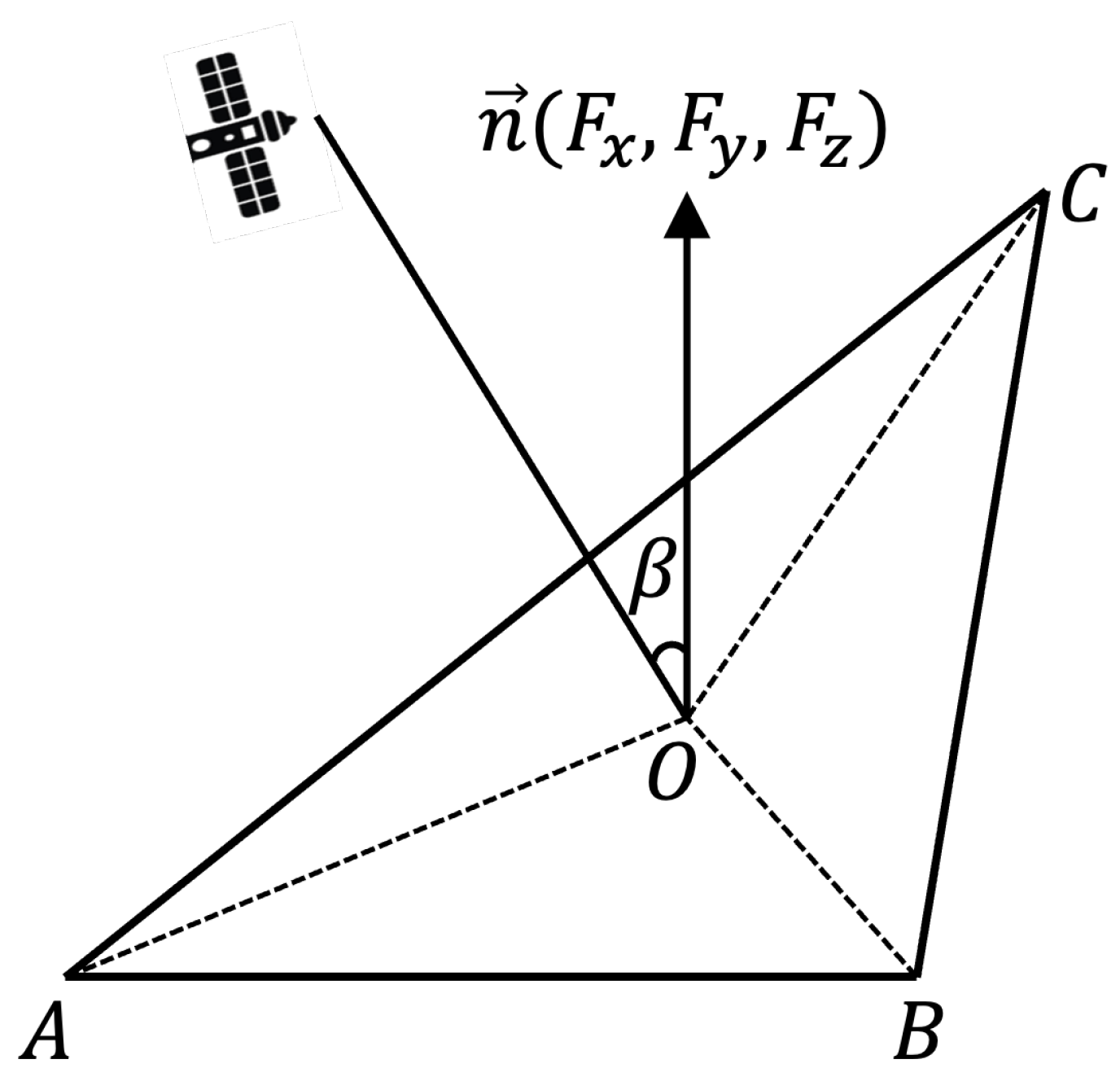
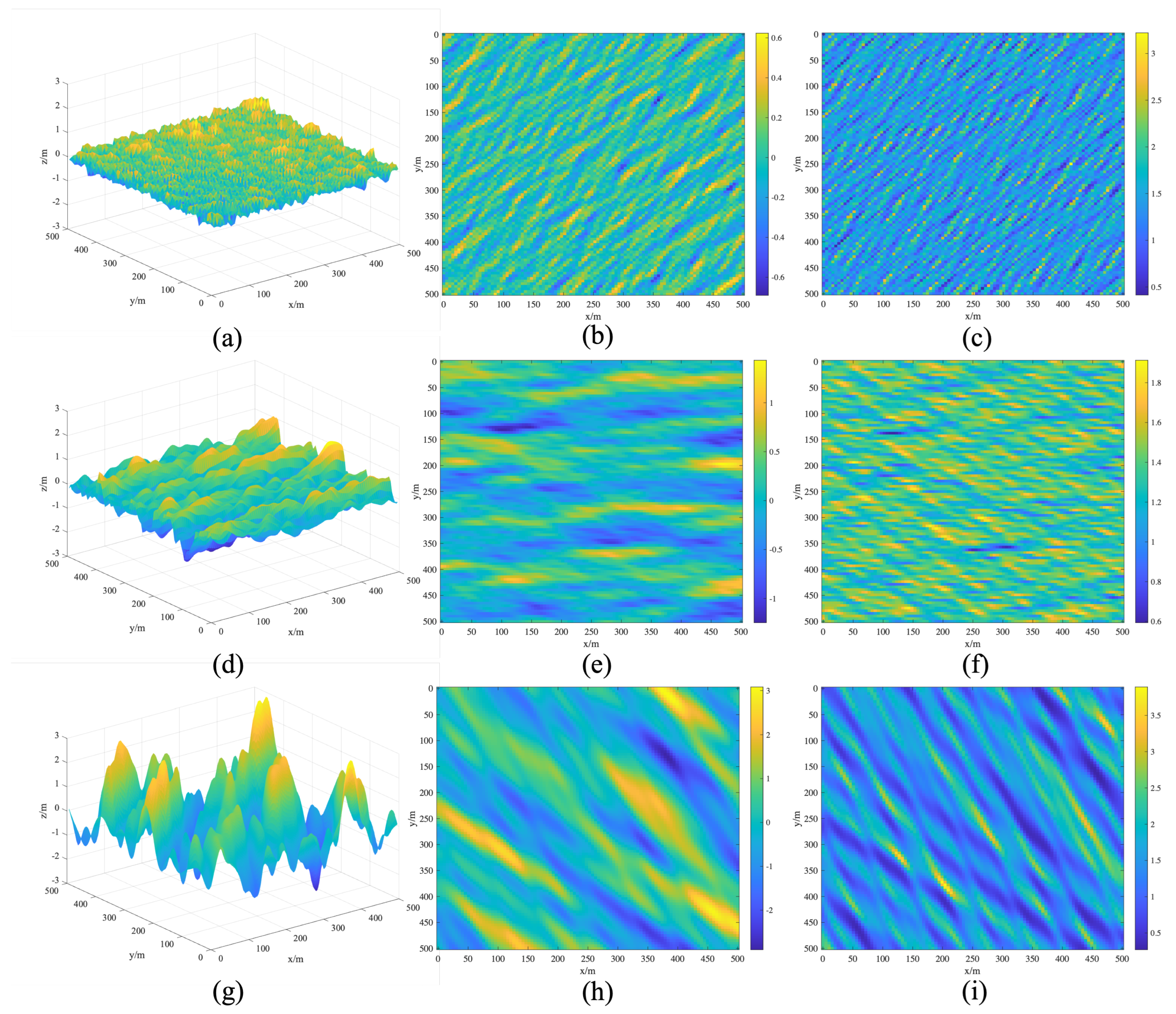
2.1. Three-Dimensional Ocean Surface Modeling System

The mathematical modeling of the ocean surface serves as the foundation for almost all remote sensing parameter inversion challenges related to the ocean. This paper mainly utilizes the ocean surface Doppler spectrum model to describe ocean motion. In 2000, Romeiser and Thompson proposed a new model for the simulation of Doppler spectra and ATI signatures, which is based on Bragg scattering theory in a composite surface model method [14]. This model has been validated to have the ability to reduce computation times by more than one order of magnitude compared to the predictions of an established model based on fundamental electrodynamic expressions, without losing consistency. Compared with the ocean surface current model, the ocean surface Doppler spectrum model is more suitable for the ATI-SAR ocean surface current inversion algorithm, since the interferometric phase in ATI-SAR images is a measurement of the Doppler shift of the backscattered signal and thus of the radial velocity of the ocean surface scatters, as mentioned before. Consequently, the three-dimensional ocean surface model constructed in this subsection is mainly based on the principle of the ocean surface Doppler spectrum model proposed by Romeiser and Thompson, involving the three-dimensional time-varying ocean surface modeling and the corresponding electromagnetic scattering modeling.

The three-dimensional ocean surface model is constructed by overlaying a height spectrum function, resembling the actual ocean surface, onto a two-dimensional wave spectrum $s\left(\omega ,\theta \right)$ comprising a wave spectrum model $s\left(\omega \right)$ and a direction function $\psi \left(\theta \right)$:

$$s\left(\omega ,\theta \right)=s\left(\omega \right)·\psi \left(\theta \right),$$

(1)

where $\omega$ represents frequency and $\theta$ is the angle between the wind direction and the current direction. Given that the wave spectrum is generated through the superposition of multiple cosine wave vectors with varying amplitudes and frequencies, a three-dimensional time-varying ocean surface equation can be derived by employing the linear superposition method to delineate the three-dimensional coordinates of each scattering point on the dynamic ocean surface:

$$\left\{\begin{array}{c}x\left(t\right)={\displaystyle \sum _{i=1,j=1}^{M,N}}\left\{\delta ·M-a_{i}sin\left[{\displaystyle \frac{{\omega }_i^2}{g}}(\delta ·Mcos{\theta }_i+\eta ·Nsin{\theta }_i)-{\omega }_{i}t+{\gamma }_i\right]\right\}\hfill \\ y\left(t\right)={\displaystyle \sum _{i=1,j=1}^{M,N}}\left(\eta ·N\right)\hfill \\ z\left(t\right)={\displaystyle \sum _{i=1,j=1}^{M,N}}{a}_{i}cos\left[{\displaystyle \frac{{\omega }_i^2}{g}}(\delta ·Mcos{\theta }_i+\eta ·Nsin{\theta }_i)-{\omega }_{i}t+{\gamma }_i\right]\hfill \end{array}\right.,$$

(2)

where $\delta$ and $\eta$ represent the fixed step length of the specified ocean surface range direction and azimuth direction, respectively, M and N determine the size of the ocean surface, $a_i$ is a random Gaussian variable with a fixed variance value representing the ocean wave height, ${\omega }_i$ represents the frequency component of the wave spectrum, ${\theta }_i$ is the angle between the wave crest and the range direction of the ocean surface, and ${\gamma }_i$ represents the random phase of the wave spectrum conforming to the uniform distribution. The three-dimensional ocean surface modeling system integrates classical wave spectra like Neumann, Pierson–Moskowitz (PM), A. K. Fung, and Jonswap, along with directional distribution functions such as Elfouhaily, Donelan-Banner, Longuet-Higgins [31,32,33,34,35,36,37], among others, providing flexibility based on the characteristics of the specific ocean region. In this paper, the PM wave spectrum and the Longuet-Higgins directional function are selected to establish the three-dimensional ocean surface. Their expressions are given by Equation (3) and Equation (4), respectively, as follows:

$$S_{PM}\left(\omega \right)={\displaystyle \frac{8.1\times {10}^{-3}{g}^2}{{\omega }^5}}exp\left(-0.74{\left({\displaystyle \frac{g}{V_{wind}\omega }}\right)}^4\right),$$

(3)

$$G_{LH}\left(k,\psi \right)={\displaystyle \frac{{\left|cos\left(\frac{\psi -{\psi }_{\omega }}{2}\right)\right|}^{2s}}{{\int }_{-\pi }^{\pi }{cos}^{2s}\left(\frac{\psi }{2}\right)d\psi }},$$

(4)

where $V_{wind}$ represents the wind speed, k is the wave number, ${\psi }_{\omega }$ is the angle of wind direction, and s is a constant.

The modeling of electromagnetic scattering on the ocean surface is a crucial step. In order to better accommodate the dynamic changes of the ocean surface, as illustrated in Figure 2, an important enhancement involves further dividing traditional rectangular scattering units into triangular ones and concentrating energy at the center of gravity O. The normal vector $\overrightarrow{n}(F_x,F_y,F_z)$ of the scattering unit can be easily derived from the coordinates of its three vertices. By considering the angle $\beta$ between the line connecting the platform and point O and the normal vector $\overrightarrow{n}(F_x,F_y,F_z)$, we can derive an expression for the local friction angle $\alpha$:

$$\alpha ={\displaystyle \frac{\pi }{2}}-arccos\left[{\displaystyle \frac{F_x+F_z·tan\left(\beta \right)}{1+{tan}^2\left(\beta \right)·\left(F_x^2+F_y^2+F_z^2\right)}}\right].$$

(5)

According to Guinard et al. [38], the backscattering coefficient under vertical polarization and horizontal polarization can be obtained based on Equation (5), as shown in Equations (6) and (7), respectively, as follows:

$${\sigma }_{VV}\left(\alpha \right)={\displaystyle \frac{3}{2}}\pi ·{10}^{-3}{\left|{\displaystyle \frac{\left(\epsilon -1\right)\left[\epsilon ·\left({cos}^2\left(\alpha \right)+1\right)-{cos}^2\left(\alpha \right)\right]}{{\left(\epsilon ·sin\left(\alpha \right)+\sqrt{\left|\epsilon -{cos}^2\left(\alpha \right)\right|}\right)}^2}}\right|}^2{tan}^4\left(\alpha \right),$$

(6)

$${\sigma }_{HH}\left(\alpha \right)={\displaystyle \frac{3}{2}}\pi ·{10}^{-3}{\left|{\displaystyle \frac{\epsilon -1}{{\left(sin\left(\alpha \right)+\sqrt{\left|\epsilon -{cos}^2\left(\alpha \right)\right|}\right)}^2}}\right|}^2{tan}^4\left(\alpha \right),$$

(7)

where $\epsilon$ is the dielectric constant related to the radar frequency.

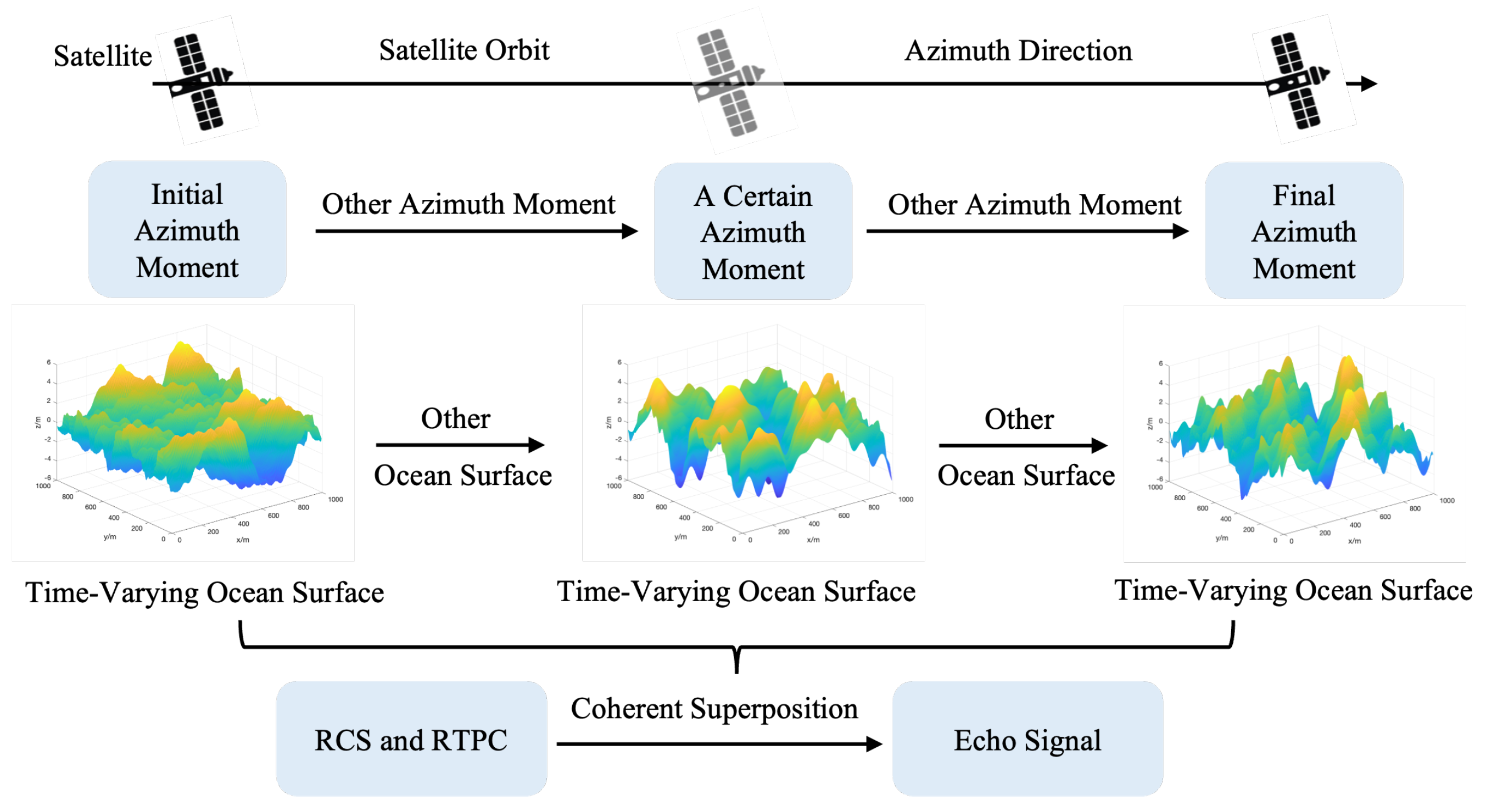
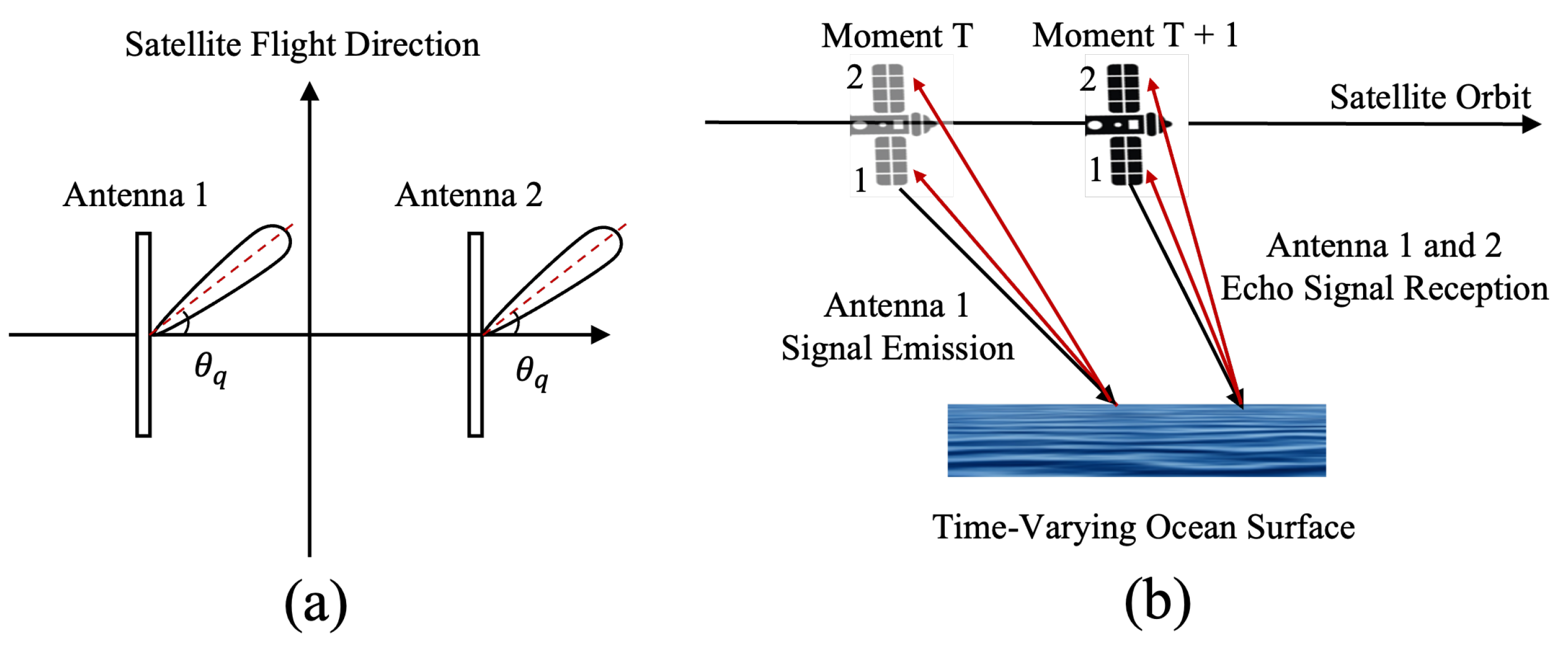
2.2. Spaceborne ATI-SAR Time-Varying Ocean Surface Echo Simulation System

In practical scenarios, the ocean surface undergoes temporal changes, and thus the ocean surface constructed in Section 2.1 also varies with time. Consequently, adjustments are necessary in the SAR echo simulation process. The system adopts the range time-domain pulse coherent (RTPC) method [39], as illustrated in Figure 3. It treats the satellite platform as “transient” between azimuth moments and generates a “frozen” three-dimensional ocean surface at each azimuth moment for calculating the backward scattering coefficient. During this process, radar transmits pulse signals to the ocean surface and receives their echoes. This sequence is repeated at subsequent azimuth moments, with the echo signals from each azimuth moment coherently combined to yield a comprehensive time-varying ocean surface echo signal.

In the context of any dual-antenna configuration, as depicted in Figure 4, the satellite platform’s motion direction aligns with the Y-axis, and the phase center of the two antennas is linked through origin O. ${\theta }_x$ and ${\theta }_z$ represent the angles between this connection and the X- and Z-axes, while ${\phi }_1$ and ${\phi }_2$ denote the downward-looking angles of antennas 1 and 2, respectively. Additionally, ${\theta }_{q1}$ and ${\theta }_{q2}$ indicate squint angles, whereas $d_1$ and $d_2$ signify their respective distances from the phase center to origin O. These parameters can be adjusted based on specific antenna configurations.

The key to the RTPC algorithm for simulating echo in any dual-antenna configuration lies in determining the azimuthal time difference of a target illuminated by the phase centers of antennas 1 and 2, which also serves as the origin of the interference phase. As depicted in Figure 5, consideration has been given to the height of a scatter point target T on the ocean surface, with its X- and Y-axis coordinates denoted as $X_T$ and $Y_T$, respectively, being related to squint angle ${\theta }_{q1}$, ${\theta }_{q2}$ and downward-looking angle ${\phi }_1$, ${\phi }_2$. According to geometric relationships, the azimuth distance difference between the target illuminated by antenna 1 and antenna 2 can be inferred as Equation (8):

$$Y_{delay}=\sqrt{R_2^2-{\left(X_T+d_2·cos\left({\theta }_x\right)\right)}^2-H^2}+d_2·sin\left({\theta }_x\right)-Y_T,$$

(8)

where $R_2$ is the distance between the phase center of antenna 2 and the delayed irradiation point on the same horizontal line of scatter point target T. Based on Equation (4), the expressions of the echoes $S_1$ and $S_2$ captured by the two antennas for scatter point target T can be obtained as follows:

$$S_1={\sigma }_T·exp\left(j·{\varphi }_1\right)·\left(\left|t_r-t{d}_1\right|\le \raisebox{1ex}{$T_r$}\!\left/ \!\raisebox{-1ex}{$2$}\right.\right)·\left(\left|t_a\right|\le \raisebox{1ex}{$T_s$}\!\left/ \!\raisebox{-1ex}{$2$}\right.\right),$$

(9)

$$S_2={\sigma }_T·exp\left(j·{\varphi }_2\right)·\left(\left|t_r-t{d}_2\right|\le \raisebox{1ex}{$T_r$}\!\left/ \!\raisebox{-1ex}{$2$}\right.\right)·\left(\left|t_a-\raisebox{1ex}{$Y_{\mathit{delay}}$}\!\left/ \!\raisebox{-1ex}{$2V$}\right.\right|\le \raisebox{1ex}{$T_s$}\!\left/ \!\raisebox{-1ex}{$2$}\right.\right).$$

(10)

In Equations (9) and (10), ${\sigma }_T$ represents the backscattering coefficient of the scatter point target T. The phases of the two echoes are denoted by ${\varphi }_1$ and ${\varphi }_2$, while $t_r$ and $t_a$ refer to the range and azimuth time, respectively. $t{d}_1$ and $t{d}_2$ indicate the time delay of the two echoes, and $T_r$ and $T_a$ represent the total sampling time. Additionally, V signifies the platform velocity. As indicated by Equation (10), variations in azimuth direction time between the two echoes lead to imaging delay, resulting in the interferometric phase [40].

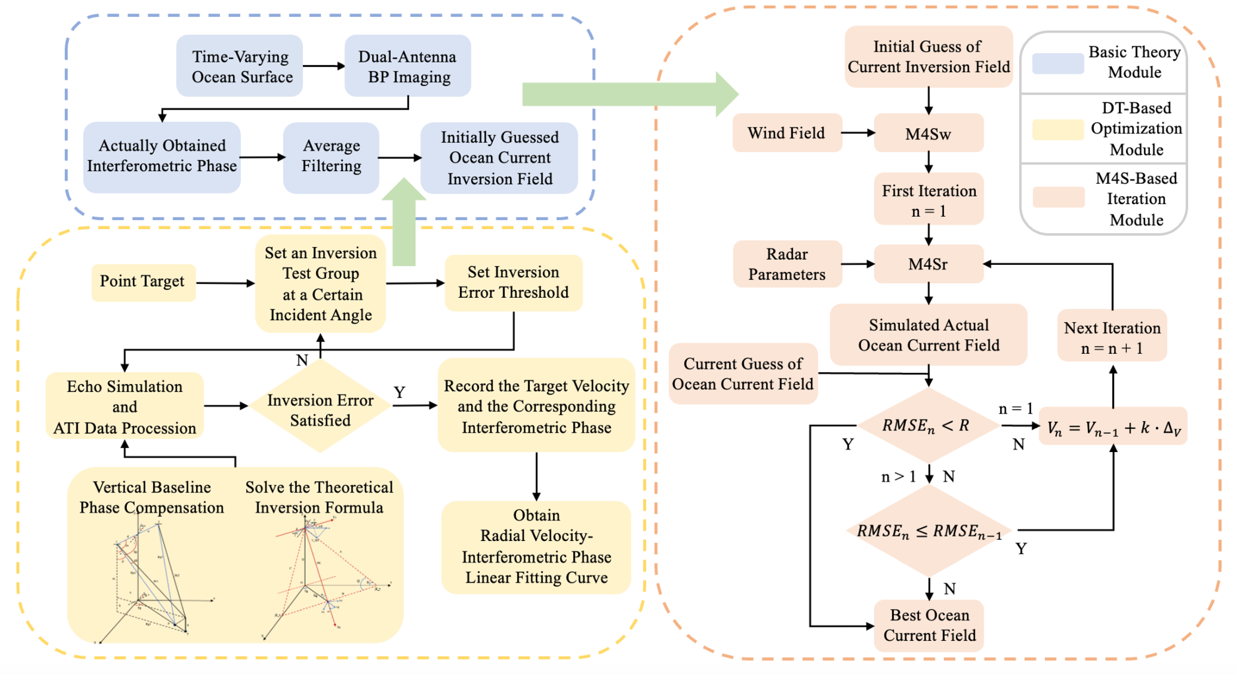
2.3. Ocean Surface Current Fitting Inversion System

This subsystem plays a critical role in the spaceborne ATI-SAR Digital Twin system of ocean surface current velocity inversion built in this paper. As mentioned in Section 1, it is challenging to accurately account for the random inversion error under any dual-antenna configuration. In specific scenarios, the conventional ATI-SAR inversion algorithm may not align perfectly with the observation geometry and system parameters, resulting in fluctuating inversion errors. In line with the concept of Digital Twin, a framework featuring the fitting inversion method for ocean surface current velocity inversion is proposed in this section. At the core of this method lies the use of a fitting approach based on Digital Twin to derive a theoretical radial velocity-interference phase fitting curve that accommodates system errors, thereby minimizing inversion errors.

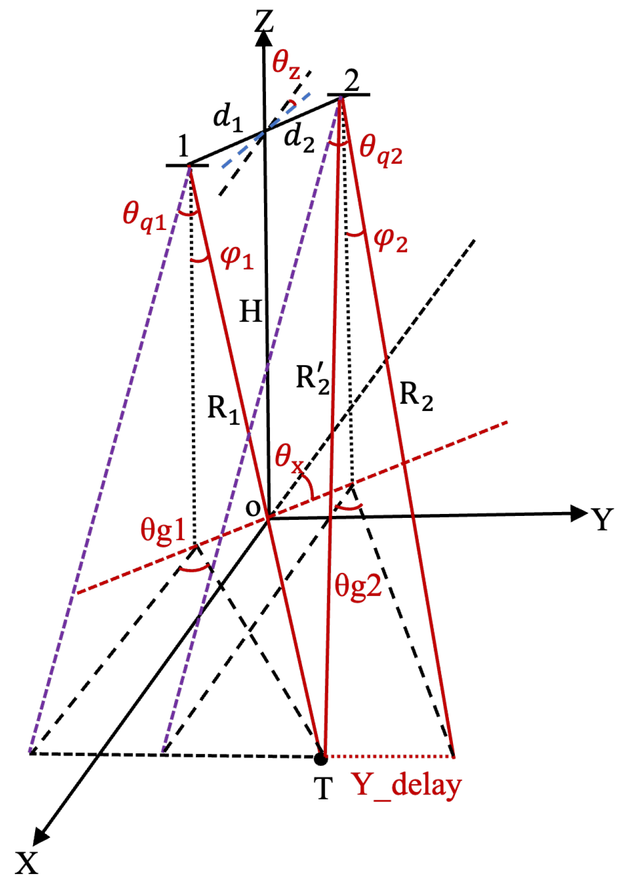
2.3.1. Basic Theory Module

As illustrated in Figure 6, the framework mainly consists of three parts. The basic theory module is the conventional method for obtaining the initially guessed current field. Through the three-dimensional ocean surface modeling system and the spaceborne ATI-SAR time-varying ocean surface echo simulation system established in Section 2.1 and Section 2.2, respectively, the actually obtained interferometric phase can be extracted from the dual-antenna back projection (BP) images [41]. After the average filtering, the initially guessed current inversion field $V^0$ can be obtained through Equation (11) [42]:

$$V^0=-{\displaystyle \frac{\lambda V}{4\pi Bsin{\theta }_{in}}}{\varphi }^0,$$

(11)

where ${\varphi }^0$ represents the actually obtained interferometric phase, B represents the effective baseline length, and ${\theta }_{in}$ represents the incident angle. In simulation, the theoretical interferometric phase ${\varphi }_{cal}$ can be obtained by Equation (12):

$${\varphi }_{cal}=-{\displaystyle \frac{2\pi B{V}_r}{\lambda V}},$$

(12)

where $V_r$ is the simulated radial velocity of the ocean surface current.

2.3.2. M4S-Based Iteration Module

The M4S-based iteration module aims to eliminate velocity interference since the velocities obtained in Equation (12) are Doppler velocities, which are the vector sum of the target in all observation areas as given in Equation (13):

$$V_{Doppler}=V_c+V_{wind}+V_o+V_b+V_e,$$

(13)

where $V_c$ represents the ocean surface current field, $V_{wind}$ represents the velocity caused by the ocean wind, $V_o$ represents the large-scale wave orbital velocity, $V_b$ represents the Bragg wave phase velocity, and $V_e$ represents the fluctuating velocity error stemming from the mismatch between the ATI-SAR algorithm and various antenna configurations mentioned in Section 1. $V_c$ and $V_{wind}$ are the components needed, while $V_o$ and $V_b$ are supposed to be eliminated by M4S iteration. The M4S software (version 3.2.0) was developed by Romeiser et al. [14] at Hamburg University, Germany for numerical simulations of the microwave radar imaging of ocean surface current features and wind features near the ocean surface, which lead to signatures in radar images. It mainly consists of two calculation modules, namely, M4Sw and M4Sr [43]. The former is responsible for calculating spatially varying surface wave spectra, while the latter generates corresponding radar images based on the system parameters and operating modes. The version of the M4S software used in this paper is 3.2.0. The specific M4S-based iteration algorithm is as follows:

Step 1: The parameters required in the iteration process should be initialized. n is the number of iterations. R represents the threshold of root mean square error (RMSE), which is used as the error evaluation index in iteration and is defined by Equation (14):

$$RMSE=\sqrt{{\displaystyle \frac{1}{n}}\sum _{i=1}^n{(V_i-{\widehat{V}}_i)}^2},$$

(14)

where $V_i$ and ${\widehat{V}}_i$ represent the simulated actual ocean current field and the iteratively inverted current field, respectively.

Step 2: The initially guessed current inversion field obtained in basic theory module and the wind field are thrown into the M4Sw to generate the corresponding wave spectrum. After that, the M4sr continues the calculation with given radar parameters to obtain the simulated actual ocean current field.

Step 3: Determine whether the guessed current field needs to be corrected. The guessed current field should be compared with the actual ocean current field. If the RMSE of the current field is less than R, the iteration should be stopped. By this time, the guessed current field is supposed to be the best ocean current field. Otherwise, the guessed current field needs to be corrected through Equation (15):

$$V_n=V_{n-1}+k·{\Delta }_V,$$

(15)

where $V_n$ and $V_{n-1}$ represent the ocean current field of the current iteration and of the last iteration, respectively, k represents the pixel difference between the simulated actual current field and the guessed current field, and ${\Delta }_V$ is the correction value which is defined in Equation (16):

$${\Delta }_V={\displaystyle \frac{4\pi \alpha Bsin{\theta }_{in}}{\lambda V}},$$

(16)

where $\alpha$ is an empirical constant based on the number and accuracy of iterations, and $\lambda$ is the radar wavelength. After the correction of the guessed current field, the iteration is continued until the RMSE is less than the threshold, or it diverges.

2.3.3. DT-Based Optimization Module

The DT-based optimization module is the core of the framework. The fitting inversion method proposed in this module aims to optimize the actually obtained interferometric phase after average filtering in the basic theory module to eliminate the velocity error $V_e$ in Equation (13). Through the radial velocity-interference phase fitting curve, abnormal points of the interference phase that significantly deviate from the theoretical value will be adjusted to fit with the curve, which effectively improves the issue of fluctuating error in the initially guessed current field and reduces the average inversion error for the best ocean current field after the M4S-based iteration. The specific algorithm for obtaining the radial velocity-interference phase fitting curve is as follows:

Step 1: Determine the dual-antenna configuration and system parameters in the very beginning. After that, apply a rough adjustment to the ATI-SAR inversion algorithm based on the echo simulation algorithm of any dual-antenna configuration in Section 2.2 under the given system parameters.

Step 2: Set a group of point targets for inversion testing with varying radial velocities, positions, and backscattering coefficients. Additionally, set a crucial inversion error threshold that directly influences the performance of the subsequent fitting inversion method. It is essential that this threshold should surpass the anticipated inversion error for optimal results.

Step 3: Inversion of the point target test group is carried out according to the preliminarily adjusted ATI-SAR inversion algorithm in Step 1. If the inversion error is less than the threshold, the radial velocity and interference phase corresponding to the point target in the set of experiments is retained as one of the fitting points for subsequent analysis. Otherwise, this set of experimental data is discarded.

Step 4: After obtaining enough fitting point data, linear fitting is carried out to obtain the radial velocity-interference phase fitting curve.

It is necessary to note that the ATI processing of point target echo data in Figure 6 incorporates the phase compensation caused by the baseline perpendicular to the track, as the target velocity only affects the interferometric phase caused by the along-track baseline. The same compensation is required for the actually obtained interferometric phase in time-varying ocean surface current inversion. The formula for the phase compensation ${\varphi }_{ver}$ in any antenna configuration is directly provided below as follows:

$${\varphi }_{ver}=-{\displaystyle \frac{2\pi h}{\lambda R}}·\left(B_x{\displaystyle \frac{cos\alpha }{sin(\beta +(\alpha -\beta )/2)}}+B_z{\displaystyle \frac{sin\alpha }{sin(\beta +(\alpha -\beta )/2)}}\right).$$

(17)

If the platform is moving along the Y-axis, $B_x$ and $B_z$ represent the components of the baseline on the X- and Z-axes, respectively. Additionally, h denotes the target’s altitude above sea level. $\alpha$ indicates the angle between the main antenna-target line and the Z-axis, while $\beta$ represents the angle between the main antenna-BP imaging projection point line and the Z-axis. Consequently, the actually obtained interferometric phase ${\varphi }_{al}$ caused by the radial velocity of the ocean current is Equation (18):

$${\varphi }_{al}={\varphi }_{all}-{\varphi }_{ver},$$

(18)

where ${\varphi }_{all}$ represents the mixed interferometric phase.

3. Simulation Experiment and Analysis of Results

In this section, a simulation example of ocean surface current inversion for spaceborne ATI-SAR with an unconventional antenna configuration is demonstrated. The system parameters are fed into the Digital Twin system established in Section 2. Under diverse ocean surface conditions, including varying wind speed and direction, ocean surface current velocities categorized as low, medium, and high are retrieved to assess the effectiveness of the Digital Twin system.

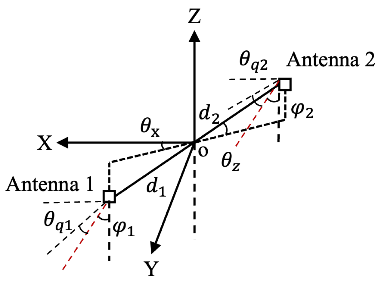
3.1. Antenna Configuration and System Parameters

The dual-antenna configuration and operational mode for the simulation example in this section are depicted in Figure 7. The former significantly varies from the setup of traditional ATI-SAR. Both antennas are positioned at the same horizontal level, with their physical baseline perpendicular to the satellite’s flight direction. In comparison with Figure 4, both ${\theta }_x$ and ${\theta }_z$ are zero, the squint angle and downward-looking angle of the two antennas are identical, and the distance between the phase center of the two antennas and the origin O is also equal. In the operational mode, a one-shot and double-receive approach is employed, where antenna 1 transmits electromagnetic signals and antennas 1 and 2 receive echo signals. The specific simulation system parameters are provided in

Table 1. Main parameters of simulation system.

System Parameter	Value	System Parameter	Value
Satellite velocity	7700 m/s	Operating frequency	9.65 GHz
Orbital altitude	438.7 km	Bandwidth	75 MHz
Incident angle	35°	Effective along-track baseline length	5.4645 m
Range sampling points	3290	Sampling rate in range direction	90 MHz
Azimuth sampling points	2637	PRF	4000 Hz
Squint angle	3°	Receiver noise figure	5 dB
Mean wave height	0 m	Wind direction variance	0.5
System azimuth resolution	2 m	System range resolution	2 m
Azimuth BP grid resolution	2 m	Range BP grid resolution	2 m
Azimuth ocean surface grid resolution	2 m	Range ocean surface grid resolution	2 m
Simulated ocean surface range	500 m × 500 m	BP imaging range	490 m × 490 m

. It should be noted that the simulated ATI-SAR works at X-band with a 3° squint angle and an effective along-track baseline of 5.4645 m.

3.2. Simulation Outcomes and Analysis

In order to fully demonstrate the performance of the spaceborne ATI-SAR Digital Twin system of ocean surface current velocity inversion proposed in this paper, this section sets nine groups of ocean surface parameters as shown in

Table 2. Parameters of ocean surface and ocean current velocity.

Experimental Group	1	2	3	4	5	6	7	8	9
Wind direction (°)	45	90	135	45	45	45	135	135	135
Wind speed (m/s)	5	10	15	5	10	15	10	10	10
Radial ocean current velocity (m/s)	0.5	1.0	1.5	1.0	1.0	1.0	0.5	1.0	1.5

. These groups can be divided into three subgroups for different purposes. Groups 1 to 3 represent three classical ocean surface conditions at different wind direction, namely, low wind speed with low radial current velocity, medium wind speed with medium radial current velocity, and high wind speed with high radial current velocity. This subgroup is mainly set to evaluate the overall performance of the framework proposed in Section 2. Groups 4 to 6 are set to evaluate the effect of wind speed on the performance of the framework, where the wind direction and radial current velocity are set to a fixed value. Groups 7 to 9 are set to evaluate whether the varying radial current velocity has an influence on the performance of the framework or not, where the wind direction and wind speed are set to a fixed value. Additionally, the effect of the wind direction can also be evaluated by comparing the simulation outcomes of groups 2, 5, and 8.

In the very beginning, based on the classical PM wave spectrum and Longuet-Higgins direction function, a three-dimensional ocean surface model was established in the three-dimensional ocean surface modeling system mentioned in Section 2.1 under the conditions of ocean surface parameters presented in Table 2. Figure 8 shows the modeling results of a certain azimuth moment, encompassing the three-dimensional ocean surface, the two-dimensional ocean surface top view heat map, and its backscattering coefficient. It should be noted that only the results of groups 1 to 3 are presented in Figure 8 due to their representativeness and space limitations. Additionally, the scale in Figure 8 shows the simulated ocean surface range of $500\mathrm{m}\times 500\mathrm{m}$ in azimuth and range direction, which is provided in Table 1. It can be distinctly observed that the amplitude and direction of ocean surface currents are modulated by wind speed and wind direction.

Based on the 3D ocean surfaces depicted in Figure 8, dual-channel time-varying ocean surface echo signals can be acquired via the spaceborne ATI-SAR ocean surface echo simulation system established in Section 2.2. Subsequently, nine sets of dual-channel ocean surface BP images can be derived by applying the BP imaging algorithm. The simulation parameters for BP imaging is given in Table 1. It is observed that the BP imaging range is slightly smaller than the simulated ocean surface range, as the time-varying ocean surface at the boundary hinders the accuracy of the inversion results and is deemed unnecessary. Additionally, the BP grid resolution in azimuth and range direction is consistent with system resolution and ocean surface grid resolution in order to achieve the best inversion results. As the BP images of both channels are consistent in the shape of the ocean current, only the image of channel 1 is presented in each group, as illustrated in Figure 9. It should be noted that the scale in Figure 9 represents the BP grid cell in range and azimuth direction, and so does the scale in Figure 10, Figure 11, Figure 12, Figure 13, Figure 14 and Figure 15.

The phase difference of each set of dual-channel BP images is extracted, and the corresponding original interferometric phase can be obtained through vertical phase compensation based on Equations (17) and (18). To facilitate comparison, the experimental results of three subgroups are presented separately. For each subgroup, $99\times 99$ pixel units in the middle of the three groups of actually obtained interferometric phase are selected and presented together, and the results are shown in Figure 10.

It is evident that a considerable error exists between the actually obtained interferometric phase and the theoretical interferometric phase. This is partially attributed to the phase interference resulting from clutter velocity such as the Bragg wave phase velocity and large-scale wave orbital velocity, and partially due to the fluctuation matching error between the ATI-SAR algorithm and the observed geometry. The former primarily relies on the subsequent processing of the M4S-based iteration algorithm mentioned in Section 2.3.2, while for the latter, the fitting method presented in Section 2.3.3 can be adopted to preprocess the actually obtained interference phase and eliminate the abnormal matching error to a certain extent. Based on Figure 6, a set of point targets for the radial velocity-interference phase fitting curve was established. Under the condition where the velocity inversion error threshold was 0.02 m/s, the fitting data presented in

Table 3. Radial velocity-interference phase data fitting point.

Theoretical Radial Velocity (m/s)	Interferometric Phase (°)	Inversed Radial Velocity (m/s)	Inversion Error (m/s)
0	−0.0003	0.0002	0.0002
0.3046	−0.0875	0.2901	−0.0146
0.6092	−0.1827	0.6056	−0.0037
0.9138	−0.2695	0.8940	−0.0198
1.2185	−0.3657	1.2121	−0.0064
1.5231	−0.4509	1.5047	−0.0184
1.8277	−0.5493	1.8206	−0.0070
2.2023	−0.6323	2.2159	−0.0136

were obtained, and linear fitting was conducted to eventually obtain the fitting curve depicted in Figure 11. The figure has preliminarily demonstrated its error correction effect in point target inversion. The small yellow triangle in the figure represents some abnormal error points caused by the observation geometric matching error, which can be well corrected by employing the fitting curve.

Figure 12 presents the theoretical current field obtained based on Equation (11) and its mean profile in range direction. Figure 13, Figure 14 and Figure 15 exhibit the initially guessed ocean current field obtained before and after the interference phase optimization based on the fitting curve presented in Figure 11, of subgroup 1, subgroup 2, and subgroup 3, respectively.

It can be clearly observed that the fitting inversion method has an obvious optimization effect on the initially guessed ocean current field. Particularly in the scenarios of high wind speed and high ocean surface current radial velocity, a large number of abnormal inversion points that are significantly beyond the standard value due to algorithm matching errors and ocean surface movements are corrected to the position near the theoretical value. Nevertheless, the results obtained at this point are still mingled with clutter velocity such as Bragg wave velocity and large-scale wave orbital velocity. In order to focus on the effectiveness of the DT-based fitting inversion method and achieve higher inversion accuracy, further iteration of the ocean current field through the M4S-based iteration module is necessary.

Table 4. M4S iteration data before fitting curve optimization.

Experimental Group	Iteration Round	RMSE before Divergence
1	7	0.0936
2	7	0.1147
3	9	0.1524
4	7	0.0968
5	8	0.1278
6	9	0.1497
7	7	0.1136
8	7	0.1157
9	7	0.1185

and

Table 5. M4S iteration data after fitting curve optimization.

Experimental Group	Iteration Round	RMSE before Divergence
1	5	0.0913
2	6	0.0968
3	7	0.1153
4	5	0.0932
5	6	0.0824
6	8	0.1121
7	5	0.0899
8	5	0.0913
9	5	0.0967

show the iterative process data of the ocean current field before and after the fitting curve optimization of the original ocean current field, respectively, with the RMSE threshold set to 0.1. The reduction in the iteration round and the value of RMSE signifies the optimization of the DT-based fitting inversion method. In order to quantitatively evaluate the optimization effect, Figure 16, Figure 17 and Figure 18 show the results of the best ocean current field after iteration before and after fitting curve optimization. It can be observed that in this simulation experiment, the fitting inversion method based on the Digital Twin system proposed in this paper has indeed improved the final inversion performance. The results of subgroup 1 show that the final inversion errors are 0.0014 m/s, 0.0074 m/s, and 0.0143 m/s, respectively, with the classical combination of wind speed and radial current velocity, which have been decreased by 0.0365 m/s, 0.0408 m/s, and 0.0430 m/s compared with the inversion results before fitting curve optimization. Additionally, the results of subgroup 2 show that under the conditions of fixed wind direction and radial current velocity, the final inversion errors are 0.0037 m/s, 0.0081 m/s, and 0.0176 m/s at low, medium, and high wind speed, respectively, which have been decreased by 0.0370 m/s, 0.0411 m/s, and 0.0401 m/s after fitting curve optimization. Finally, the results of subgroup 3 show that under the conditions of fixed wind direction and wind speed, the final inversion errors are 0.0069 m/s, 0.0077 m/s, and 0.0084 m/s at low, medium, and high radial ocean current velocity, respectively, which have been decreased by 0.0384 m/s, 0.0408 m/s, and 0.0423 m/s after the fitting curve optimization.

Based on Figure 16 and the analysis above, several conclusions can be obtained. First of all, the DT-based framework for spaceborne ATI-SAR ocean current velocity inversion has indeed improved the overall performance of current velocity inversion under the condition of unconventional ATI-SAR dual-antenna configuration. The average inversion error is 0.0084 m/s, showcasing a reduction of 0.0401 m/s before the optimization of the DT-based fitting inversion method within the framework. Secondly, whether from a qualitative or quantitative point of view, the final inversion error is relatively large in the case of high wind speed and high ocean current radial velocity, because the higher the ocean surface wind speed and current velocity, the larger the surge amplitude, the more complex the ocean surface motion, the greater the ocean surface coherence error and observation geometric error, and ultimately the larger the inversion error. This is consistent with the actual situation. Additionally, the wind direction seems to have little obvious influence on the inversion result comparing the inversion results between groups 2, 5, and 8.

4. Conclusions and Discussion

In this paper, a spaceborne ATI-SAR Digital Twin system framework for ocean surface current inversion is proposed, which is capable of conducting 3D ocean surface modeling, time-varying ocean surface echo simulation, and radial velocity inversion of ocean surface current. The aim of this system framework is to address the issue of abnormal inversion errors resulting from the non-ideal effective along-track baseline and thus the possible mismatch between the adjusted ATI-SAR algorithm and the actual observation geometry under any dual-antenna configuration. Through proposing a Digital Twin-based fitting inversion approach incorporated into the system, the corresponding radial velocity-interference phase fitting curve is obtained to optimize the original ocean current field, effectively eliminating most of the abnormal interference phase error points. Subsequently, the final iterated ocean current field can be obtained through a M4S-based iteration module in the framework. A simulation example of a spaceborne ATI-SAR ocean surface current inversion with an unconventional dual-antenna configuration, which is significantly different from the classical spaceborne ATI-SAR dual-antenna configuration, validates the effectiveness of the Digital Twin method proposed in this paper.

However, ocean surface motion in reality is far more complex than the random motion in simulation, and the existing 3D ocean surface modeling technology fails to achieve complete correspondence between physical and virtual entities in the concept of Digital Twin. In future research, the Digital Twin system constructed in this paper will be continuously improved based on the factors above.

The potential of the application of the concept of Digital Twin on ocean information inversion is unlimited. This paper mainly focuses on the application on ATI-SAR ocean current inversion, while ocean information is abundant, such as wind, ocean wave, and ocean gravity fields. In particular, the issue of simultaneous and precise inversion of ocean surface wind and current information based on ATI-SAR mode has been a research hotspot in the recent decade. It is promising that the DT-based system framework proposed in this paper could offer a solution to issues like that after proper improvement in the near future.

References

1. Elyouncha, A.; Eriksson, L.E.B.; Romeiser, R.; Ulander, L.M.H. Measurements of Sea Surface Currents in the Baltic Sea Region Using Spaceborne Along-Track InSAR. IEEE Trans. Geosci. Remote Sens. 2019, 57, 8584–8599. [Google Scholar] [CrossRef]
2. Vachon, W. Current measurement by Lagrangian drifting buoys-problems and potential. In Proceedings of the OCEANS’77 Conference Record, Los Angeles, CA, USA, 17 October 1977; pp. 639–645. [Google Scholar]
3. Kovačević, V.; Gačić, M.; Poulain, P.M. Eulerian current measurements in the Strait of Otranto and in the Southern Adriatic. J. Mar. Syst. 1999, 20, 255–278. [Google Scholar] [CrossRef]
4. Moreira, A.; Prats-Iraola, P.; Younis, M.; Krieger, G.; Hajnsek, I.; Papathanassiou, K.P. A tutorial on synthetic aperture radar. IEEE Geosci. Remote Sens. Mag. 2013, 1, 6–43. [Google Scholar] [CrossRef]
5. Goldstein, R.M.; Zebker, H. Interferometric radar measurement of ocean surface currents. Nature 1987, 328, 707–709. [Google Scholar] [CrossRef]
6. Thompson, D.R.; Jensen, J. Synthetic aperture radar interferometry applied to ship-generated internal waves in the 1989 Loch Linnhe experiment. J. Geophys. Res. Ocean. 1993, 98, 10259–10269. [Google Scholar] [CrossRef]
7. Graber, H.C.; Thompson, D.R.; Carande, R.E. Ocean surface features and currents measured with synthetic aperture radar interferometry and HF radar. J. Geophys. Res. Ocean. 1996, 101, 25813–25832. [Google Scholar] [CrossRef]
8. Romeiser, R. Current measurements by airborne along-track InSAR: Measuring technique and experimental results. IEEE J. Ocean. Eng. 2005, 30, 552–569. [Google Scholar] [CrossRef]
9. Toporkov, J.V.; Perkovic, D.; Farquharson, G.; Sletten, M.A.; Frasier, S.J. Sea surface velocity vector retrieval using dual-beam interferometry: First demonstration. IEEE Trans. Geosci. Remote Sens. 2005, 43, 2494–2502. [Google Scholar] [CrossRef]
10. Romeiser, R.; Suchandt, S.; Runge, H.; Steinbrecher, U.; Grunler, S. First analysis of TerraSAR-X along-track InSAR-derived current fields. IEEE Trans. Geosci. Remote Sens. 2009, 48, 820–829. [Google Scholar] [CrossRef]
11. Weydahl, D.; Sagstuen, J.; Dick, Ø.; Rønning, H. SRTM DEM accuracy assessment over vegetated areas in Norway. Int. J. Remote Sens. 2007, 28, 3513–3527. [Google Scholar] [CrossRef]
12. Zhang, B.; Perrie, W.; Li, X.; Pichel, W.G. Mapping sea surface oil slicks using RADARSAT-2 quad-polarization SAR image. Geophys. Res. Lett. 2011, 38. [Google Scholar] [CrossRef]
13. Qingjun, Z. System design and key technologies of the GF-3 satellite. Acta Geod. Et Cartogr. Sin. 2017, 46, 269. [Google Scholar]
14. Romeiser, R.; Thompson, D.R. Numerical study on the along-track interferometric radar imaging mechanism of oceanic surface currents. IEEE Trans. Geosci. Remote Sens. 2000, 38, 446–458. [Google Scholar] [CrossRef]
15. Romeiser, R.; Runge, H. Theoretical evaluation of several possible along-track InSAR modes of TerraSAR-X for ocean current measurements. IEEE Trans. Geosci. Remote Sens. 2006, 45, 21–35. [Google Scholar] [CrossRef]
16. Romeiser, R.; Runge, H.; Suchandt, S.; Kahle, R.; Rossi, C.; Bell, P.S. Quality assessment of surface current fields from TerraSAR-X and TanDEM-X along-track interferometry and Doppler centroid analysis. IEEE Trans. Geosci. Remote Sens. 2013, 52, 2759–2772. [Google Scholar] [CrossRef]
17. Romeiser, R.; Runge, H.; Suchandt, S.; Sprenger, J.; Weilbeer, H.; Sohrmann, A.; Stammer, D. Current measurements in rivers by spaceborne along-track InSAR. IEEE Trans. Geosci. Remote Sens. 2007, 45, 4019–4031. [Google Scholar] [CrossRef]
18. Mittermayer, J.; Alberga, V.; Buckreuss, S.; Riegger, S. TerraSAR-X: Predicted performance. In Proceedings of the Sensors, Systems, and Next-Generation Satellites VI, SPIE, Barcelona, Spain, 8–10 September 2003; Volume 4881, pp. 244–255. [Google Scholar]
19. Mittermayer, J.; Runge, H. Conceptual studies for exploiting the TerraSAR-X dual receive antenna. In Proceedings of the IGARSS 2003, 2003 IEEE International Geoscience and Remote Sensing Symposium, Proceedings (IEEE Cat. No. 03CH37477), Toulouse, France, 21–25 July 2003; Volume 3, pp. 2140–2142. [Google Scholar]
20. Kahle, R.; Runge, H.; Ardaens, J.S.; Suchandt, S.; Romeiser, R. Formation flying for along-track interferometric oceanography—First in-flight demonstration with TanDEM-X. Acta Astronaut. 2014, 99, 130–142. [Google Scholar] [CrossRef]
21. Gini, F.; Lombardini, F. Multibaseline cross-track SAR interferometry: A signal processing perspective. IEEE Aerosp. Electron. Syst. Mag. 2005, 20, 71–93. [Google Scholar] [CrossRef]
22. Grilli, S.T. Depth inversion in shallow water based on nonlinear properties of shoaling periodic waves. Coast. Eng. 1998, 35, 185–209. [Google Scholar] [CrossRef]
23. Klemas, V. Remote sensing of ocean internal waves: An overview. J. Coast. Res. 2012, 28, 540–546. [Google Scholar] [CrossRef]
24. Xu, Z.; Zhang, H.; Wang, Y.; Wang, X.; Xue, S.; Liu, W. Dynamic detection of offshore wind turbines by spatial machine learning from spaceborne synthetic aperture radar imagery. J. King Saud Univ.-Comput. Inf. Sci. 2022, 34, 1674–1686. [Google Scholar] [CrossRef]
25. Tao, F.; Zhang, H.; Liu, A.; Nee, A.Y.C. Digital Twin in Industry: State-of-the-Art. IEEE Trans. Ind. Inform. 2019, 15, 2405–2415. [Google Scholar] [CrossRef]
26. Rouffet, T.; Poisson, J.B.; Hottier, V.; Kemkemian, S. Digital twin: A full virtual radar system with the operational processing. In Proceedings of the 2019 International Radar Conference (RADAR), Toulon, France, 23–27 September 2019; pp. 1–5. [Google Scholar]
27. Timoshenko, A.V.; Perlov, A.Y.; Kazantsev, A.M.; Khodataev, N.A.; Lvov, K.V. Methodology for the Development of a Digital Twin of Radar Stations of a Functional Block Structure. In Proceedings of the 2022 Systems of Signal Synchronization, Generating and Processing in Telecommunications (SYNCHROINFO), Arkhangelsk, Russia, 29 June–1 July 2022; pp. 1–4. [Google Scholar]
28. Karboski, A.; Vivekanandan, J.; Burghart, C.; Eret, T. Airborne Polarimetric Doppler Phased Array Weather Radar: Digital Twin of the Active Electronically Scanned Array. In Proceedings of the 2022 IEEE International Symposium on Phased Array Systems and Technology (PAST), Waltham, MA, USA, 11–14 October 2022; pp. 1–6. [Google Scholar]
29. Xie, W.; Qi, F.; Liu, L.; Liu, Q. Radar Imaging Based UAV Digital Twin for Wireless Channel Modeling in Mobile Networks. IEEE J. Sel. Areas Commun. 2023, 41, 3702–3710. [Google Scholar] [CrossRef]
30. Grieves, M. Digital twin: Manufacturing excellence through virtual factory replication. White Pap. 2014, 1, 1–7. [Google Scholar]
31. Neumann, G. On wind-generated wave motion at subsurface levels. Eos. Trans. Am. Geophys. Union 1955, 36, 985–992. [Google Scholar]
32. Pierson, W.J., Jr.; Moskowitz, L. A proposed spectral form for fully developed wind seas based on the similarity theory of SA Kitaigorodskii. J. Geophys. Res. 1964, 69, 5181–5190. [Google Scholar] [CrossRef]
33. Fung, A.; Lee, K. A semi-empirical sea-spectrum model for scattering coefficient estimation. IEEE J. Ocean. Eng. 1982, 7, 166–176. [Google Scholar] [CrossRef]
34. Hasselmann, D.E.; Dunckel, M.; Ewing, J. Directional wave spectra observed during JONSWAP 1973. J. Phys. Oceanogr. 1980, 10, 1264–1280. [Google Scholar] [CrossRef]
35. Elfouhaily, T.; Chapron, B.; Katsaros, K.; Vandemark, D. A unified directional spectrum for long and short wind-driven waves. J. Geophys. Res. Ocean. 1997, 102, 15781–15796. [Google Scholar] [CrossRef]
36. Donelan, M.A.; Hamilton, J.; Hui, W. Directional spectra of wind-generated ocean waves. Philos. Trans. R. Soc. London. Ser. A Math. Phys. Sci. 1985, 315, 509–562. [Google Scholar]
37. Longuet-Higgins, M.S. Observation of the directional spectrum of sea waves using the motions of a floating buoy. Oc. Wave Spectra 1963. [Google Scholar]
38. Guinard, N.; Daley, J. An experimental study of a sea clutter model. Proc. IEEE 1970, 58, 543–550. [Google Scholar] [CrossRef]
39. Mori, A.; De Vita, F. A time-domain raw signal simulator for interferometric SAR. IEEE Trans. Geosci. Remote Sens. 2004, 42, 1811–1817. [Google Scholar] [CrossRef]
40. Wollstadt, S.; Lopez-Dekker, P.; De Zan, F.; Younis, M. Design principles and considerations for spaceborne ATI SAR-based observations of ocean surface velocity vectors. IEEE Trans. Geosci. Remote Sens. 2017, 55, 4500–4519. [Google Scholar] [CrossRef]
41. Yegulalp, A.F. Fast backprojection algorithm for synthetic aperture radar. In Proceedings of the 1999 IEEE Radar Conference. Radar into the Next Millennium (Cat. No. 99CH36249), Waltham, MA, USA, 22 April 1999; pp. 60–65. [Google Scholar]
42. Kim, D.J.; Moon, W.; Moller, D.; Imel, D. Measurements of ocean surface waves and currents using L- and C-band along-track interferometric SAR. IEEE Trans. Geosci. Remote Sens. 2003, 41, 2821–2832. [Google Scholar]
43. Romeiser, R.; Breit, H.; Eineder, M.; Runge, H.; Flament, P.; De Jong, K.; Vogelzang, J. On the suitability of TerraSAR-X split antenna mode for current measurements by along-track interferometry. In Proceedings of the IGARSS 2003, 2003 IEEE International Geoscience and Remote Sensing Symposium, Proceedings (IEEE Cat. No. 03CH37477), Toulouse, France, 21–25 July 2003; Volume 2, pp. 1320–1322. [Google Scholar]
Figure 1. Spaceborne ATI-SAR ocean surface current inversion Digital Twin system framework.
Remotesensing 16 03739 g001
Figure 2. Observation geometry between spaceborne ATI-SAR platform and ocean surface triangular scattering unit.
Remotesensing 16 03739 g002
Figure 3. Time−varying ocean surface echo simulation system.
Remotesensing 16 03739 g003
Figure 4. Any dual-antenna configuration.
Remotesensing 16 03739 g004
Figure 5. Observation geometry of RTPC algorithm.
Remotesensing 16 03739 g005
Figure 6. Framework of ocean surface current fitting inversion system based on Digital Twin.
Remotesensing 16 03739 g006
Figure 7. Antenna configuration and operational mode: (a) antenna configuration; (b) operational mode.
Remotesensing 16 03739 g007
Figure 8. 3D modeling outcomes of the ocean surface: (a) Group 1 3D ocean surface. (b) Group 1 2D ocean surface top view heat map. (c) Group 1 backscattering coefficient. (d) Group 2 3D ocean surface. (e) 2D ocean surface top view heat map. (f) Group 2 backscattering coefficient. (g) Group 3 3D ocean surface. (h) Group 3 2D ocean surface top view heat map. (i) Group 3 backscattering coefficient.
Remotesensing 16 03739 g008
Figure 9. BP images of ocean surface: (a) Group 1. (b) Group 2. (c) Group 3. (d) Group 4. (e) Group 5. (f) Group 6. (g) Group 7. (h) Group 8. (i) Group 9.
Remotesensing 16 03739 g009
Figure 10. Interference phase: (a) Theoretical interference phase. (b) Actually obtained interference phase in subgroup 1. (c) Actually obtained interference phase in subgroup 2. (d) Actually obtained interference phase in subgroup 3.
Remotesensing 16 03739 g010
Figure 11. Radial velocity−interference phase fitting curve based on Digital Twin.
Remotesensing 16 03739 g011
Figure 12. Theoretical ocean surface current field: (a) Theoretical current field of three kinds of radial velocity. (b) Mean profile in range direction of the theoretical current field.
Remotesensing 16 03739 g012
Figure 13. Comparison of the initially guessed ocean current field before and after fitting curve optimization in subgroup 1: (a) Before fitting curve optimization. (b) Mean profile in range direction before fitting curve optimization. (c) After fitting curve optimization. (d) Mean profile in range direction after fitting curve optimization.
Remotesensing 16 03739 g013
Figure 14. Comparison of the initially guessed ocean current field before and after fitting curve optimization in subgroup 2: (a) Before fitting curve optimization. (b) Mean profile in range direction before fitting curve optimization. (c) After fitting curve optimization. (d) Mean profile in range direction after fitting curve optimization.
Remotesensing 16 03739 g014
Figure 15. Comparison of the initially guessed ocean current field before and after fitting curve optimization in subgroup 3: (a) Before fitting curve optimization. (b) Mean profile in range direction before fitting curve optimization. (c) After fitting curve optimization. (d) Mean profile in range direction after fitting curve optimization.
Remotesensing 16 03739 g015
Figure 16. Comparison of the best iterative ocean current field before and after fitting curve optimization in subgroup 1.
Remotesensing 16 03739 g016
Figure 17. Comparison of the best iterative ocean current field before and after fitting curve optimization in subgroup 2.
Remotesensing 16 03739 g017
Figure 18. Comparison of the best iterative ocean current field before and after fitting curve optimization in subgroup 3.
Remotesensing 16 03739 g018