Reconstructing a Fine Resolution Landscape of Annual Gross Primary Product (1895–2013) with Tree-Ring Indices

Abstract

Low carbon management and policies should refer to local long-term inter-annual carbon uptake. However, most previous research has only focused on the quantity and spatial distribution of gross primary product (GPP) for the past 50 years because most satellite launches, the main GPP data source, were no earlier than 1980. We identified a close relationship between the tree-ring index (TRI) and vegetation carbon dioxide uptake (as measured by GPP) and then developed a nested TRI-GPP model to reconstruct spatially explicit GPP values since 1895 from seven tree-ring chronologies. The model performance in both phases was acceptable: We chose general regression neural network regression and random forest regression in Phase 1 (1895–1937) and Phase 2 (1938–1985). With the simulated and real GPP maps, we observed that the GPP for grassland and overall GPP were increasing. The GPP landscape patterns were stable, but in recent years, the GPP’s increasing rate surpassed any other period in the past 130 years. The main local climate driver was the Palmer Drought Severity Index (PDSI), and GPP had a significant positive correlation with PDSI in the growing season (June, July, and August). With the GPP maps derived from the nested TRI-GPP model, we can create fine-scale GPP maps to understand vegetation change and carbon uptake over the past century.

1. Introduction

A substantial amount of greenhouse gasses is emitted by human activities contributing to global warming and the increasing frequency of extreme weather [1,2]. High levels of CO₂ emission have disrupted the equilibrium between carbon sink and carbon source [3]. Many researchers have examined historical records or applied mathematical models to reconstruct early anthropogenic carbon emissions [4,5], but few studies have evaluated the quantity or spatial distribution of carbon sinks over a long temporal period. Currently, satellite imagery is the main source to monitor or quantitatively estimate the amount and the spatial distribution of the gross primary product (GPP) or net primary product (NPP), two key metrics to evaluate the storage of carbon sinks [6,7]. However, most optical satellite launches were later than the 1980s. It was inaccessible to obtain GPP landscape patterns via satellites earlier than 50 years ago [8]. Tree rings, an ideal proxy for dating, have three advantages in GPP reconstruction. Firstly, tree-ring width reflects tree growth and energy conversion via photosynthesis (GPP) [9]. Secondly, tree rings record tree growth annually, so the temporal resolution of GPP data is 1 year. Lastly, trees are globally widespread, so we can use tree rings to reconstruct GPP around the world.

Some dendrochronology studies have investigated the relationship between vegetation indices and tree-ring width [10,11]. Wang et al. [12], by employing a linear regression model to reconstruct NPP with tree-ring indices (TRI), demonstrated a positive relationship. Liang et al. [13] determined that the tree-ring index (TRI) had a strong relationship with NDVI in grassland close to the collection plot. Most studies treated an entire study area as a singular dot, and the reconstruction was at a very coarse scale. But in reality, there is still a heterogeneous landscape with many forests, grasslands, or water patches in one study site, which were completely ignored by those studies. Li et al. [14] achieved an NDVI reconstruction with tree-ring indices at a fine scale with a spatial resolution of 30 m. But their study had obvious limitations in balancing the number of plots involved in the study and the temporal extent of their study when the reconstruction time was constrained to the temporal overlap of the trees on the plots. The more plots that are involved, the shorter the reconstruction time that was available in the common period. Our research generated annual GPP fine-scale maps since 1895, and the nested reconstruction approach enabled us to use the full time period of the individual chronologies.

2. Methods

The whole study time was divided into three phases: Phase 1 (1895–1937), Phase 2 (1938–1985), and Phase 3 (1986–2013). The training set included GPP values from 1986 and tree-ring indices (TRI) of multiple plots from 1986 to 2013. For Phase 1 and Phase 2, we trained the GPP–TRI models individually and chose the best models for these two phases (Figure 1).

2.1. Study Areas

Our study is located across the boundary of Illinois and Indiana, in the Midwest U.S. (Figure 2). The whole area covers 3510 km² (117 km × 30 km), ranging from 36.97°N to 42.51°N in latitude and from 84.78°W to 91.51°W in longitude, located in the humid continental climate zone.

Local average temperatures in summer and winter are 24 degrees Celsius and −4 degrees, respectively. The annual precipitation is 300 mm. (https://weatherspark.com/y/13301/Average-Weather-in-Normal-Illinois-United-States-Year-Round (accessed on 13 August 2024).

Our study area covers five cities: Terre Haute (Indiana), Marshall (Illinois), Martinsville (Illinois), Casey (Illinois), and Greenup (Illinois). In our study area, there are no obvious counter-urbanization sites where former built-up areas have reverted back to forest and grassland patches, so we assume that the forest and grassland in 2013 were kept stable for the whole study period (1895–2013). According to the NLCD 2013 [15], we reclassified the whole area into five land covers: forest, grassland (including cropland), urban areas, water, and wetland. Li et al.’s research [14] demonstrated that the regression between tree-ring indices and vegetation index could work well only in grasslands and forests. So, we excluded water, wetlands, and built-up areas and only focused on grasslands and forests. The term “whole area” in later paragraphs only indicates all forest and grassland in our study site. The local dominant species include white oak (Quercus alba), red oak (Quercus rubra), shagbark hickory (Carya ovata), and sugar maple (Acer saccharum).

2.2. Date Source and Data Preprocessing

The main data sources in our study are tree-ring indices and GPP products. We collected tree-ring data from seven plots, where six of them were from the International Tree-Ring Databank (ITRDB) and one of them was from our collection in Lincoln Trail State Park, Illinois. All collected tree cores in Lincoln Trail State Park were dried in the laboratory fume hood and were sanded with progressively finer sandpaper (120, 320, and 400 grit). Then, we hand-sanded the samples with 3 M 30 ųm sanding film until no scratches were visible under the microscope [16]. The samples were scanned with an Epson V600 scanner at 2400 DPI and measured using the CooRecorder program [17] with an output of 0.001 mm precision. We checked the dating of each core against its paired tree-level core (A vs. B) in CooRecorder, built a local master with a kernel of well-dated samples, and checked the date of the rest of the samples against that kernel. We checked the quality of the measurements and the dating between cores for the whole site in CDendro [17] and COFECHA [18]. Then, the raw ring widths were detrended using an age-dependent spline for all chronologies in ARSTAN [18]. We cut off the tree-ring index (TRI) when the expressed population signal (EPS) fell below 0.85 [19]. Among those seven plots, there were two white oak plots, one sugar maple plot, one shagbark hickory plot, one tulip tree plot, one red oak plot, and one white ash plot (

Table 1. The background information of the seven selected plots.

Order	ITRDB ID	Species Name	Scientifc Name	Earliest Year	Latest Year	Available Phases
1	IL018	White Oak	Quercus alba	1847	2014	Phase 1 and Phase 2
2	IL030	Sugar Maple	Acer saccharum	1895	2016	Phase 1 and Phase 2
3	IN012	Shagbark Hickory	Carya ovata	1912	2013	Phase 2
4	IN013	Tuliptree	Liriodendron tulipifera	1920	2013	Phase 2
5	IN014	Red Oak	Quercus rubra	1892	2013	Phase 1 and Phase 2
6	IN035	White Ash	Fraxinus americana	1938	2013	Phase 2
7	Our collection	White Oak	Quercus alba	1855	2023	Phase 1 and Phase 2

Note: The earliest years of Plot 3, Plot 4, and Plot 5 were not in the range of Phase 1 (1895–1937), so they could not join Phase 1 regression.

). Among seven plots, tree-ring indices from four of them were used in Phase 1 reconstruction, and all of them were used in Phase 2.

The annual GPP data from 1986 to 2013 were from the Numerical Terradynamic Simulation Group (NTSG) [20], whose spatial resolution was 30 m and temporal resolution was 16 days. The unit of the product was g C/m⁻² year⁻¹ GPP. For each year, we chose all available GPP images in the growing season (June, July, and August) and generated annual GPP maps by averaging the values for these 3 months. Then, the non-vegetation areas (water, wetland, and built-up areas) were masked out. All data processing mentioned above was via Google Earth Engine. Though the NTSG GPP was the simulated GPP product with the Moderate Resolution Imaging Spectroradiometer (MODIS) and Landsat satellite images, the Landsat series satellite actually provided us with reliable satellite images since 1986. So, in the paper, we call the GPP product “real data”. After we simulated the GPP data prior to 1986, we called the combination of the simulated data and the real data “combined data”.

In general, there are three main climate drivers to influence vegetation photosynthesis and GPP absorption: pure temperature, pure precipitation, and the combined effect of precipitation and temperature [21]. The Palmer Drought Severity Index (PDSI) is a standardized index to evaluate regional dryness with temperature and precipitation. The index ranges from −10 to 10, where a positive index indicates more moisture. If the value is lower than −2, we define the weather as drought (https://climatedataguide.ucar.edu/climate-data/palmer-drought-severity-index-pdsi (accessed on 1 September 2024). Monthly local precipitation, temperature, and PDSI from 1895 to 2013 could be assessed via the following website (https://wrcc.dri.edu/wwdt/time/ (accessed on 13 August 2024)).

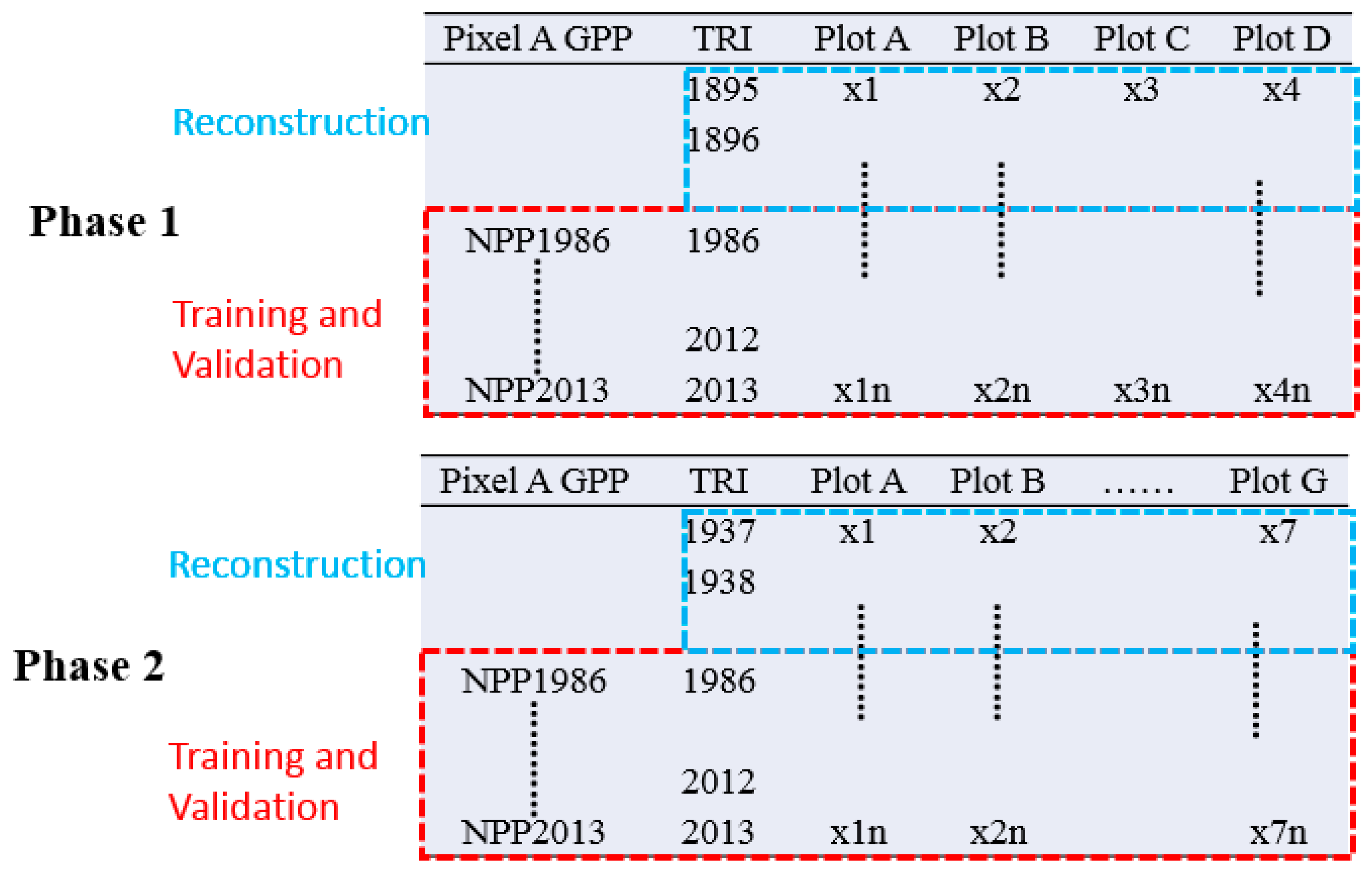
2.3. Pixel by Pixel Regression

All of our regression analyses were at the pixel level. The whole study period consisted of two sub-periods: Phase 1 and Phase 2. In Phase 2 (1938–1985), we developed the models for each pixel in our study areas between GPP values in that pixel from 1986 to 2013 and TRI of seven plots from 1986 to 2013 as our independent and dependent variables, respectively, in model training. We used 5-fold validation to evaluate the model performances (

Table 2. The 5-fold cross-validation scheme.

Order	Training Set (22)	Validation Set (6)	Validation Year
Fold 1	1992–2013	1986–1991	1990
Fold 2	1986–1990, 1997–2013	1991–1996	1995
Fold 3	1986–1995, 2002–2013	1996–2001	2000
Fold 4	1986–2000, 2007–2013	2001–2006	2005
Fold 5	1986–2007	2008–2013	2010

) where, for each pixel, there were 22 pairs of training samples (GPP and multiple TRIs) in the training sets. In Phase 1 (1895–1937), only four of them met our requirements, so we built up the models for each pixel between GPP and TRI of four plots. The reconstruction process in Phase 1 and Phase 2 was similar to each other, except that there are four available plots and seven available plots in Phase 1 and Phase 2, respectively [22]. For each phase, we explored the relationship between GPP and TRI with three models (Figure 3): Random forest regression (RF), Support Vector Machine regression (SVM), and General Regression Neural Network regression (GRNN).

Random forest (RF) regression applies the bootstrap aggregating technique and constructs multiple decision trees (100 trees in our study) at the same time. Each tree generates an individual regression algorithm, and the RF calculates the mean of all decision tree outputs. The application of RF regression is widespread in remote sensing and GIS [23,24].

The General Regression Neural Network regression (GRNN) is an improved neural network learning approach. The approach is one-pass learning algorithm with one radial basis layer and one special linear layer [25]. Single-pass learning does not need backpropagation, and the use of Gaussian function guarantees a high accuracy even though the inputs have noise. The GRNN was widely applied in many fields like soil moisture downscaling [26], urban flood mapping [27], and burn area mapping [28].

The Support Vector Machine regression (SVM) is a supervised learning algorithm to find a hyper-plane in an N-dimensional space. The ideal hyper-plane has the largest distance between two separate classes. The algorithm usually has good performance in a small training set [29]. In our study, the number of training samples for each pixel is only 28 (1986–2013), so we chose it as one of candidate models. The SVM has been a popular approach in leaf index regression [30], snow-depth retrieval [31], and forest cover change [32].

2.4. Model Evaluation

Based on model performance, we selected the best model among the three models for two phases, respectively. There are four evaluation metrics: Adjusted R² (Adj R², Equation (1)), Root Mean Squared Error (RMSE, Equation (2)), Mean Absolute Error (MAE, Equation (3)), and Mean Absolute Percentage Error (MAPE, Equation (4)).

$${\mathrm{A}\mathrm{d}\mathrm{j} \mathrm{R}}^2=1-\left({\displaystyle \frac{n-1}{n-p}}\right){\displaystyle \frac{SSE}{SST}}$$

(1)

where SSE and SST are the sum of square error and the sum of squared total, respectively; n and p are the number of samples and the number of regression coefficients, respectively. Spiess and Neumeyer [33] warned that in some cases, R square in nonlinear fitting was inappropriate.

$$\mathrm{R}\mathrm{M}\mathrm{S}\mathrm{E}=\sqrt{{\sum }_{i=1}^n{\displaystyle \frac{{(S_i-R_i)}^2}{n}}}$$

(2)

$$\mathrm{M}\mathrm{A}\mathrm{E}={\displaystyle \frac{{\sum }_{i=1}^n\left|S_i-R_i\right|}{n}}$$

(3)

$$\mathrm{M}\mathrm{A}\mathrm{P}\mathrm{E}={\displaystyle \frac{{\sum }_{i=1}^n\left|\frac{S_i-R_i}{R_i}\right|}{n}}$$

(4)

where S and R are the simulated value and real value; n is the number of samples.

We applied a 5-fold cross-validation to test model performance for two phases. From 1986 to 2013 (28 years), we chose 22-year data as our training set and the rest of the years (6 years) as the validation set. Then, we chose the data in 1 specific year among those 6 years as our validation year. We repeated the same process five times and averaged the metrics from the 5-fold validation. Then, we chose the best and reran the best model with 28 years of data.

2.5. Analysis of the Relationship between GPP and Climate Factors

We calculated the annual GPP of forest, grassland, and whole area in the growing season. We also collected monthly precipitation (mm), temperature (degrees Celsius), and PDSI. Then, we computed the correlation (Equation (5)) between GPP and those three climate factors. Some researchers have demonstrated that precipitation and temperature in previous years, like the snowpack, might still influence vegetation growth and then affect photosynthesis and GPP production [34], so we computed the correlations between GPP and the factors from previous May to current September. The GPP collection time was from June to August, so we would not calculate the correlations after September.

$$\mathrm{r}={\displaystyle \frac{{\sum }_{i=1}^n(g_i-\overline{g})(c_i-c)}{\sqrt{{\sum }_{i=1}^n{(g_i-\overline{g})}^2\sum {(c_i-\overline{c})}^2}}}$$

(5)

where g_i and c_i are the GPP value and climate factor value; $\overline{g}$ and $\overline{c}$ are mean values of the GPP series and climate factor series; and n is the number of samples.

We calculated the correlations in two datasets (long-term combined dataset and short-term dataset). If the correlation values in two datasets had substantial differences, we assume the differences come from two possible reasons. One is that the short-term dataset could not fully reflect the real situations, while the other is that the extreme climate change re-generates the current situations. No matter which reason, we will have a further investigation on the differences.

3. Results

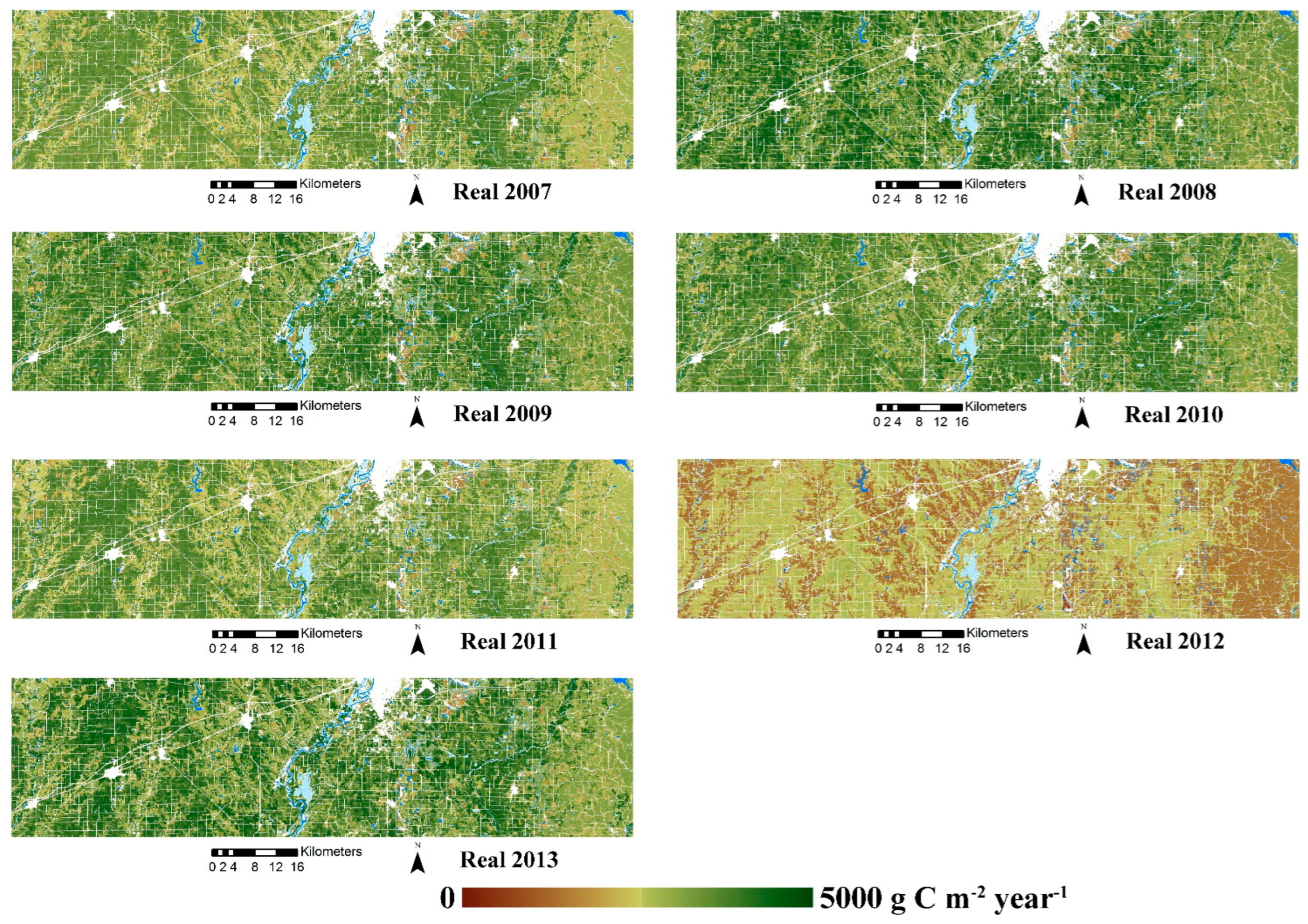
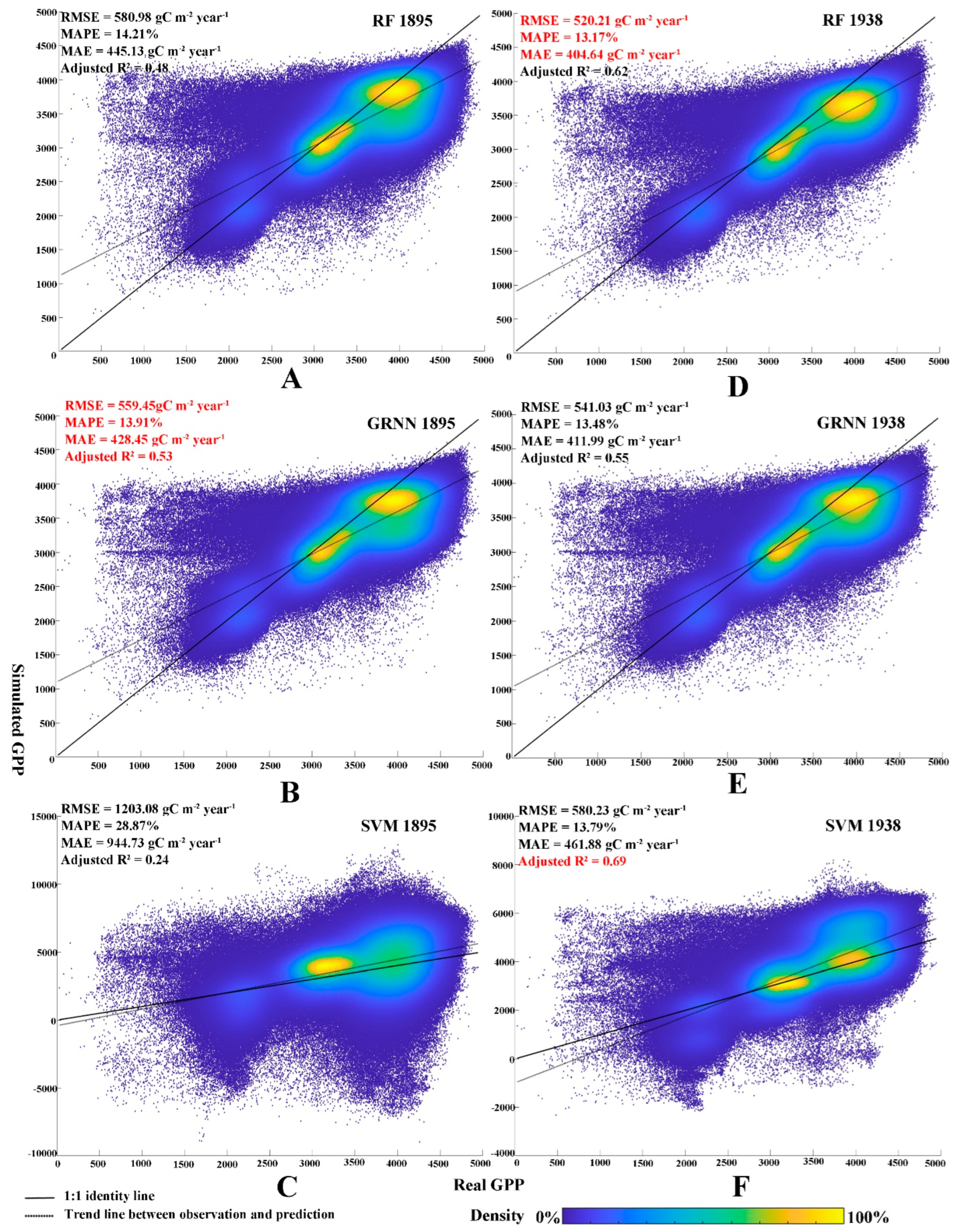
3.1. Model Performance

In both phases, we conducted three approaches (RF, GRNN, and SVM) to reconstruct GPP values and applied five validations in each phase. In Phase 1 (1895–1937), tree-ring indices (TRI) in four plots were involved in our regression (Figure 4), and the rest of the three plots did not have available data from 1895 to 1937. GRNN obviously outperformed the other approaches of RMSE, MAPE, MAE, and Adjusted R2 of GRNN were the following: 559.45 g C m⁻² year⁻¹, 13.91%, 428.45 g C m⁻² year⁻¹, and 0.53, so we chose GRNN. The SVM was the worst whose RMSE (1203.08 g C m⁻² year⁻¹) was more than twice as much as GRNN’s. In Phase 2 (1938–1985), all seven plots were used in our research. The RF had the lowest RMSE (520.21 g C m⁻² year⁻¹), the lowest MAPE (13.17%), and the lowest MAE (404.64 g C m⁻² year⁻¹), even though SVM had the highest adjusted R square (0.69). The R square could not fit non-linear curves very well, and the rest of the metrics for SVM were the worst among the three. Then, we chose RF as our best model in Phase 2 and GRNN ranked second. For the same approach, the performance in Phase 2 using seven plots was always better than that in Phase 1 using four plots where RF’s RMSE in Phase 1 and Phase 2 were 580.98 g C m⁻² year⁻¹ and 520.21 g C m⁻² year⁻¹, while GRNN RMSEs in Phase 1 and Phase 2 were 559.45 g C m⁻² year⁻¹ and 541.03 g C m⁻² year⁻¹, respectively. Even though the GRNN was the best model in Phase 1, its metrics were still worse than the RF’s (the best model in Phase 2). More details about the 5-fold validations can be found in the Appendix A.

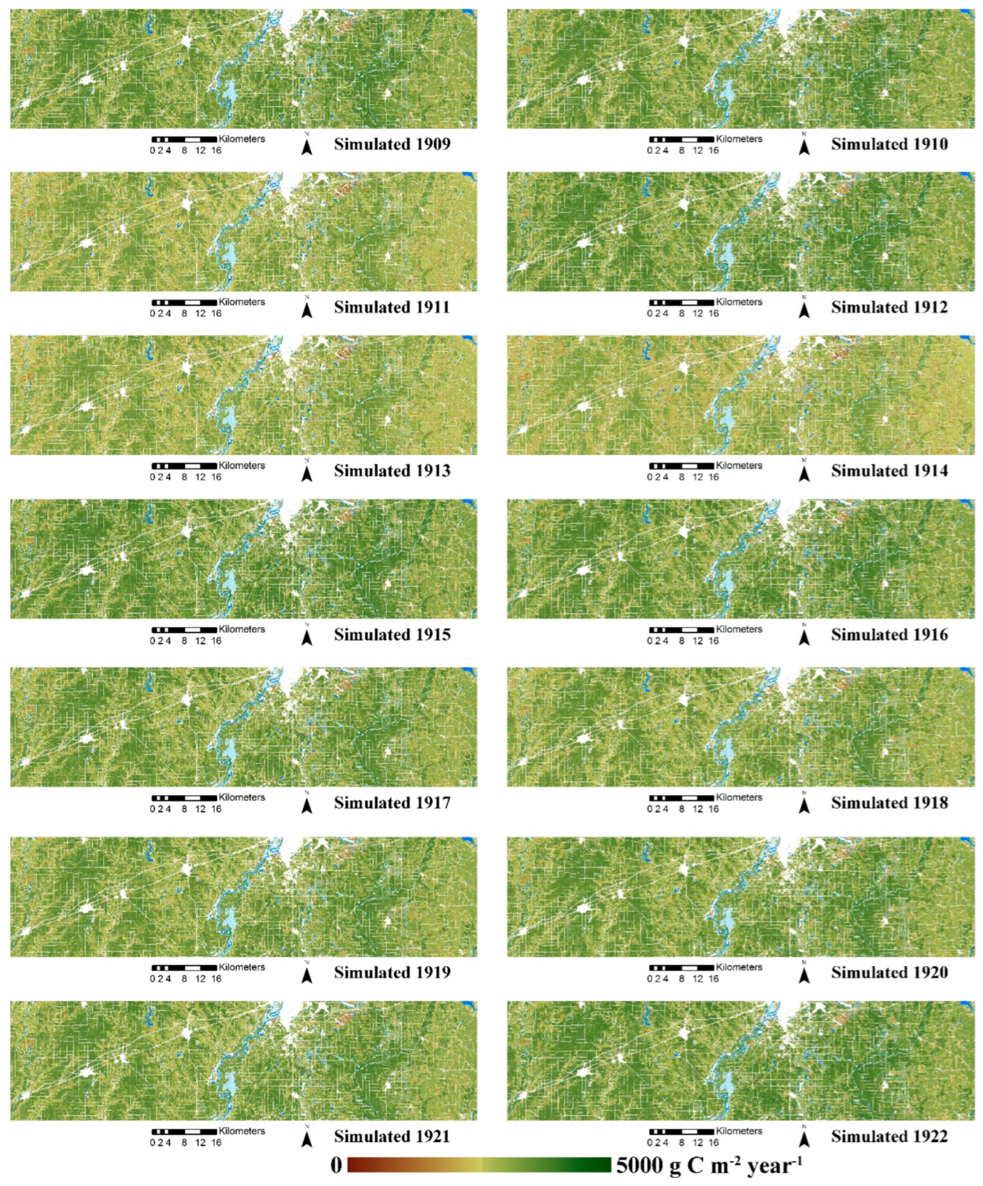
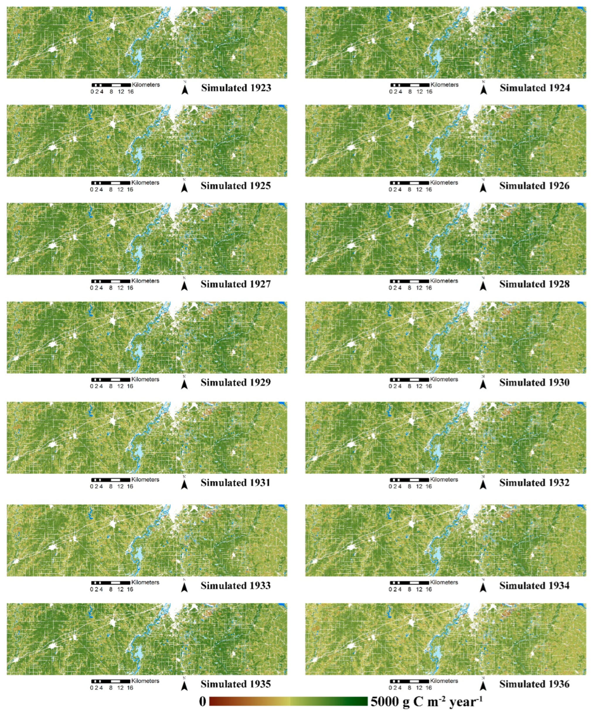
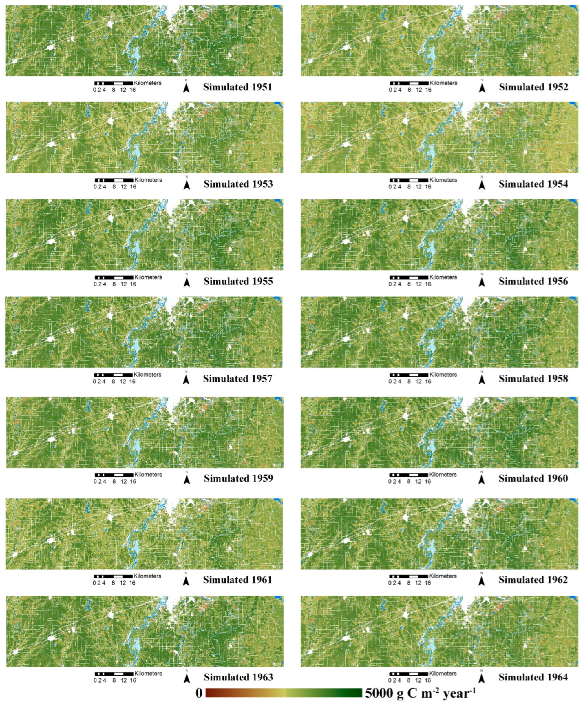
3.2. GPP Tendency in Our Study Areas

Compared to the GPP in 2013 (mean GPP = 3614.7 g C m⁻² year⁻¹), the GPP in 1895 (Figure 5A) for the whole study area was low (mean GPP = 3148.7 g C m⁻² year⁻¹), but the pattern was still very similar with the most recent one where the high GPP clusters were in the west and east of our study area. But the center was a little lower than the two sides. In 1936 (the Dust Bowl period), the average GPP was 2980.6 g C m⁻² year⁻¹. The GPP in the west of our study was decreasing while the PDSI reached −3.95 (Figure 5B). In 1954, the PDSI was −7.18, while the mean GPP was also very low (mean GPP = 2990.7 g C m⁻² year⁻¹). The landscape pattern was similar to that in 1936 (Figure 5C). In wet years like 1974, whose PDSI was 3.52, the greenness increases (mean GPP = 3337.8 g C m⁻² year⁻¹) were visible across the whole area, compared to the dry year (Figure 5D). In 2013, the moisture (PDSI = 4.09) was even higher than in 1974, while the GPP also increased to 3614.7 g C m⁻² year⁻¹. Large deep greenness patches (high GPP clusters) covered the whole area (Figure 5E). The simulated annual NPP maps can be found in Figure 5.

There were three GPP tendencies from 1895 to 2013: GPP in forest, GPP in grassland, and GPP in forest and grassland (Figure 5F). The tendency in the whole period was divided into two sub-periods: the period (1895–1985) using simulated data and the period (1986–2013) using real data. The tendency lines of GPP in grassland using combined data and GPP in the whole area using combined data were GPP = 0.2292 Year + 2931.4 and GPP = 0.1007 Year + 3041.1, whose tendency slopes were positive but flat (Figure 5F). The tendencies of GPP in grassland, and in the whole area, using only real data are positive and steep (GPP = 22.511 Year − 41,622 and GPP = 15.908 Year − 28,559). The tendency of GPP in forests with real data was contrary to that with combined data (GPP = 0.1742 Year + 3275.6; GPP = 1.7789 Year − 607.92).

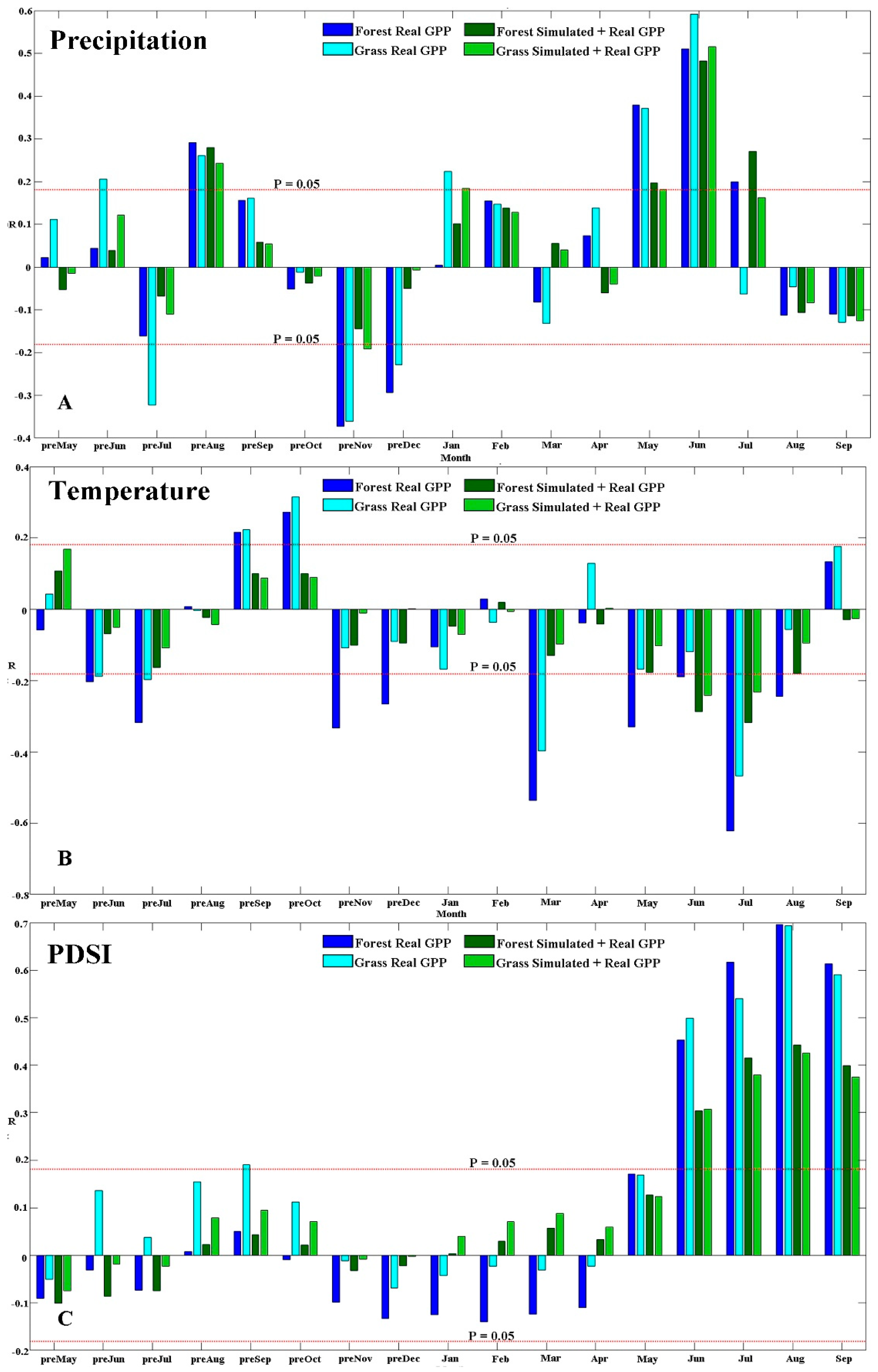
3.3. GPP and Climate

GPP production has a close relationship with the local climate. The climate in current and previous years influences the growth of plant tissues and, hence, the efficiency of photosynthesis. There are three candidate drivers to affect GPP: pure temperature, pure precipitation, and the combined effects of temperature and precipitation.

Pure precipitation could affect GPP absorption (Figure 6A). Precipitation in June had a positive relationship with GPP using real data and combined data (R forest combined June = 0.483; R grass combined June = 0.516; R forest real June = 0.511; R grass real June = 0.592). Precipitation in the previous June had a positive correlation with GPP in grassland using real data (R grass real PreJune = 0.205), but in the same month, the correlation of forest and grassland using combined data did not meet the significant level (R forest combined PreJune = 0.039; R = grass combined PreJune = 0.122).

Temperature could influence our GPP absorption (Figure 6B). The temperature in July had negative relationships with GPP in the whole study area, including forest and grassland (R forest combined July = −0.317; R grass combined July = −0.233; R forest real July = −0.623; R grass real July = −0.467). The temperature in March had positive correlations with GPP using real data (R forest real March = −0.537; R grass real March = −0.398), but in the same month, the correlation using combined data did not show significant low values (R forest combined March = −0.130; R grass combined March = −0.098).

The combined effects of temperature and precipitation could affect GPP absorption (Figure 6C). PDSI in June, July, August, and September had positive relationships with GPP in the whole study area including forest and grassland using combined data and real data. PDSI in the previous September had a positive correlation with GPP in grassland using real data (R grass real PresSep = 0.191), but in the same month, a high correlation could not be found in GPP in forest and grassland using combined data (R forest combined PresSep = 0.043; R grass combined PresSep = 0.096).

4. Discussion

4.1. Choosing the Best Models

The conventional studies considered the study site as one point where the spatial heterogeneity of the study area was neglected. But our study reconstructed GPP for every pixel in the whole area, and we also ran reconstruction models for two nested time periods (Phase 1 and Phase 2). We tried to make full use of all plots in Phase 2 and build a robust model with less error. In the meantime, we extended our study period to 1895 with fewer plots (Phase 1). In Phase 1 (1895–1937), we chose the GRNN with the highest adjusted R² and lowest RMSE, MAPE, and MAE among all three approaches. In Phase 2 (1938–1985), we selected the RF with the lowest RMSE, MAPE, and MAE. Previous researchers [14] only ran the model in Phase 1 and guaranteed model performance with as many plots as possible. They chose the intersection of all plots as their starting year, which shortened their study period. But if we intended to directly reconstruct our GPP from 1895 to 1985, we would only have four plots for the whole temporal period with more errors.

From the best model in Phase 1 and Phase 2, the performance using the best model in Phase 2 (RF) outperformed that in Phase 1 (GRNN) for all four evaluation metrics (RMSE, MAPE, MAE, and adjusted R square). Even for the same model in two phases, the model in Phase 1 was worse than that in Phase 2, which confirmed that the number of variables may determine model performance. The four metrics (RMSE, MAE, MAPE, and adjusted R square) of the two selected models were acceptable (Figure 4). Even when we compared our results with other GPP reconstruction studies using in situ data, our model performance exceeded theirs. Our RMSEs in Phase 1 and Phase 2 were 559.45 g C m⁻² year⁻¹ (1.53 g C m⁻² day⁻¹) and 520.21 g C m⁻² year⁻¹ (1.43 g C m⁻² day⁻¹), while the GPP reconstruction with eddy covariance flux towers was 2.01 g C m⁻² day⁻¹ [35]. Our study not only extended the study period but also presented the reconstruction with lower errors.

4.2. Analyzing GPP Variation over a Century

This is the first time that we witnessed the GPP spatial distribution more than 100 years ago at a fine scale. From 1895 to 2013, the landscape pattern in our study area was comparatively stable where high GPP clusters were concentrated in the west and the east of our study area (Figure 5A,D,E), but dramatic GPP changes can be found. In severe drought years (Figure 5B,C), the high GPP clusters were not visible compared to the map in 1974, but in the center of our study area, there were only some subtle GPP variations. In wet years, (Figure 4D,E), GPP was on the rise in the east and west of the study site.

The historical satellite images since 1980 could explain many variations in GPP. Our study found that GPP for grassland and for the whole area showed increasing tendencies (Figure 5F) with both datasets (combined GPP dataset and real GPP dataset). However, there are still some ecological processes like forest growth or ecological succession that may need more time to monitor [36,37]. When further studies are about local ecosystems and their restoration, the long-term dataset (combined dataset) can be more helpful. Our work demonstrates the feasibility of creating fine spatial scale GPP maps for large areas that extend over the time period of the tree-ring chronologies. As we develop longer tree-ring chronologies in a denser network, we will be able to push this type of reconstruction further back over larger areas.

In the long term (1895–2013), GPP for forests showed a decreasing tendency (GPP = −0.1007 × Year + 3041.1), while in the short term (1986–2013), the GPP tendency was increasing (GPP = 1.7789 × Year − 607.92). Even for the same increasing tendencies of GPP for grassland and for the whole area, the increasing magnitudes were also different between the long-term dataset and short-term dataset. In recent decades (1986–2013), the increasing rate was incredibly high, while during the full 119 years (1895–2013), the tendencies were flat. Our research could not judge which one was correct, but the long-term data provided us another dimension to observe GPP variation earlier over a much longer period of time. Within 119 years, we could not find any similar magnitude of GPP variations in the most recent three decades (1986–2013).

4.3. The Relationship between GPP and Climate over a Century

Even though under the influences of pure precipitation and pure temperature, GPP had a significantly high correlation with drivers in specific months like previous August precipitation, current May precipitation, current June precipitation, and temperature in July (Figure 6A,B). There were no strong seasonal precipitation responses with multiple months that remained significant. Only PDSI met the requirement when the R values in June, July, August, and September reached significance (Figure 6C). We believe that the local GPP climate driver was PDSI, the combined effects of precipitation, and temperature. Similar findings were supported by Maxwell and Harley [38], whose study area was just less than 50 km from our site. Their reconstructed PDSI in the growing season derived from tree-ring indices had a strong correlation (R = 0.77, p < 0.01).

If we only use real data to draw a conclusion about local climate, we might be misled. For example, the temperature in the previous September and October had significant positive correlations with GPP using real data, but the R values in forest and grassland were low using combined data (Figure 6B). Similar contradictions in short-term and long-term records have also been found in other studies [14]. The conclusions about climate and GPP refer to a long time series of historical records, but, simultaneously, short-term records could explain the sudden and tremendous climate change in the current time. If two data sources (the short term and long term) both indicate one tendency, the reliability could be much more than any conclusions only supported by a single dataset. If they are contrary to each other, we may need more references to make a decision. In order to have a long-term dataset, our reconstruction simulated GPP values, and then we calculated the correlations using the combined dataset.

4.4. Limitations and Future Research

With the TRI–GPP reconstruction in two phases, we confirmed that the more plots that are involved, the higher accuracy the model had (models in Phase 2 were always better than those in Phase 1). In further studies, we would collect more tree cores and increase the plot density in our study areas. From the simulated GPP values, the reconstruction of extreme values needs to be improved where some low GPP values in extreme drought could not be simulated very well. We speculated that less extreme values in training samples might lead to this issue. We tested the Convolutional Neural Network (CNN) in two small areas within our study site whose performances were worse than our chosen model due to the small sample size. We assume that if a deep-learning approach can adjust the size of our sample, the model may have a substantial improvement in future regression.

Once our model (TRI–GPP) is constructed successfully, there are two fields where we can make full use of our models. Firstly, we will enlarge our research areas into a larger area or introduce certain advanced methods. Trees are around the whole world, so in theory, we could reconstruct a long-term simulated GPP for every vegetation area and witness some long-term ecological processes, including forest succession, vegetation dynamics, and others. Secondly, we might challenge some obsolete conclusions only based on 40-year satellite images (1986–present). We also found that there were some contradictions between the short-term dataset and the long-term dataset. It is worthwhile to list the scope of both datasets where researchers should know which dataset is more appropriate to their research. But this is not the end. With the simulated GPP, we expect more updates on outmoded findings established in the old era.

5. Conclusions

With the nested TRI–GPP model, we reconstructed and mapped the spatial distribution of GPP from 1895 to 1985 in Eastern Illinois with 30 m resolution. The selected models (GRNN in Phase 1 and RF in Phase 2) performed well. The nested model was robust and could be applied to other areas to monitor GPP variation 100 years ago. Only with short-term data, some statements might be unilateral, and two datasets could present more comprehensive conclusions. Both datasets suggested that GPPs for grassland and the whole area were increasing, and high GPP clusters remained in the east and west of our study area with a relatively stable landscape pattern. The combined effects of temperature and precipitation (especially for the PDSIs in the growing season) are the local climate drivers to dominate GPP variations. While the PDSI gets higher (lower), the GPP would increase (decrease) in the west and the east of our study areas. This is the first time we have been able to visualize GPP for the past 130 years at a fine scale (30 m). With these techniques, researchers can observe annual GPP variations for centuries.

References

1. Paik, S.; Min, S.K.; Zhang, X.; Donat, M.G.; King, A.D.; Sun, Q. Determining the anthropogenic greenhouse gas contribution to the observed intensification of extreme precipitation. Geophys. Res. Lett. 2020, 47, e2019GL086875. [Google Scholar] [CrossRef]
2. Seong, M.G.; Min, S.K.; Kim, Y.H.; Zhang, X.; Sun, Y. Anthropogenic greenhouse gas and aerosol contributions to extreme temperature changes during 1951–2015. J. Clim. 2021, 34, 857–870. [Google Scholar] [CrossRef]
3. Bai, X.; Zhang, S.; Li, C.; Xiong, L.; Song, F.; Du, C.; Li, M.; Luo, Q.; Xue, Y.; Wang, S. A carbon-neutrality-capacity index for evaluating carbon sink contributions. Environ. Sci. Ecotechnol. 2023, 15, 100237. [Google Scholar] [CrossRef]
4. Lamarque, J.F.; Bond, T.C.; Eyring, V.; Granier, C.; Heil, A.; Klimont, Z.; Lee, D.; Liousse, C.; Mieville, A.; Owen, B.; et al. Historical (1850–2000) gridded anthropogenic and biomass burning emissions of reactive gases and aerosols: Methodology and application. Atmos. Chem. Phys. 2010, 10, 7017–7039. [Google Scholar] [CrossRef]
5. Henriques, S.; Borowiecki, K. The drivers of long-run CO2 emissions: A global perspective since 1800. Discuss. Pap. Bus. Econ. Univ. South. Den. 2014, 13, 1–45. [Google Scholar] [CrossRef]
6. Hou, Y.; Wang, S.; Zhou, Y.; Yan, F.; Zhu, J. Analysis of the carbon dioxide concentration in the lowest atmospheric layers and the factors affecting China based on satellite observations. Int. J. Remote Sens. 2013, 34, 1981–1994. [Google Scholar] [CrossRef]
7. Sun, Z.; Wang, X.; Zhang, X.; Tani, H.; Guo, E.; Yin, S.; Zhang, T. Evaluating and comparing remote sensing terrestrial GPP models for their response to climate variability and CO2 trends. Sci. Total Environ. 2019, 668, 696–713. [Google Scholar] [CrossRef]
8. Markham, B.L.; Helder, D.L. Forty-year calibrated record of earth-reflected radiance from Landsat: A review. Remote Sens. Environ. 2012, 122, 30–40. [Google Scholar] [CrossRef]
9. Alam, S.A.; Huang, J.G.; Stadt, K.J.; Comeau, P.G.; Dawson, A.; Gea-Izquierdo, G.; Aakala, T.; Hölttä, T.; Vesala, T.; Mäkelä, A.; et al. Effects of competition, drought stress and photosynthetic productivity on the radial growth of white spruce in western Canada. Front. Plant Sci. 2017, 8, 1915. [Google Scholar] [CrossRef]
10. Decuyper, M.; Chávez, R.O.; Čufar, K.; Estay, S.A.; Clevers, J.G.; Prislan, P.; Gričar, J.; Črepinšek, Z.; Merela, M.; Luis, M.D.; et al. Spatio-temporal assessment of beech growth in relation to climate extremes in Slovenia–An integrated approach using remote sensing and tree-ring data. Agric. For. Meteorol. 2020, 287, 107925. [Google Scholar] [CrossRef]
11. Zhou, Y.; Yi, Y.; Jia, W.; Cai, Y.; Yang, W.; Li, Z. Applying dendrochronology and remote sensing to explore climate-drive in montane forests over space and time. Quat. Sci. Rev. 2020, 237, 106292. [Google Scholar] [CrossRef]
12. Wang, T.; Bao, A.; Xu, W.; Zheng, G.; Nzabarinda, V.; Yu, T.; Huang, X.; Long, G.; Naibi, S. Dynamics of forest net primary productivity based on tree ring reconstruction in the Tianshan Mountains. Ecol. Indic. 2023, 146, 109713. [Google Scholar] [CrossRef]
13. Liang, E.; Shao, X.; Liu, H.; Eckstein, D. Tree-ring based PDSI reconstruction since AD 1842 in the Ortindag Sand Land, east Inner Mongolia. Chin. Sci. Bull. 2007, 52, 2715–2721. [Google Scholar] [CrossRef]
14. Li, H.; Thapa, I.; Speer, J.H. Fine-scale ndvi reconstruction back to 1906 from tree-rings in the greater yellowstone ecosystem. Forests 2021, 12, 1324. [Google Scholar] [CrossRef]
15. Homer, C.; Dewitz, J.; Jin, S.; Xian, G.; Costello, C.; Danielson, P.; Gass, L.; Funk, M.; Wickham, J.; Stehman, S.; et al. Conterminous United States land cover change patterns 2001–2016 from the 2016 national land cover database. ISPRS J. Photogramm. Remote Sens. 2020, 162, 184–199. [Google Scholar] [CrossRef] [PubMed]
16. Speer, J.H. Fundamentals of Tree-Ring Research; University of Arizona Press: Tucson, AZ, USA, 2010. [Google Scholar]
17. Maxwell, R.S.; Larsson, L.A. Measuring tree-ring widths using the CooRecorder software application. Dendrochronologia 2021, 67, 125841. [Google Scholar] [CrossRef]
18. Cook, E.R. A Time Series Analysis Approach to Tree Ring Standardization (Dendrochronology, Forestry, Dendroclimatology, Autoregressive Process); The University of Arizona: Tucson, AZ, USA, 1985. [Google Scholar]
19. Wigley, T.M.; Briffa, K.R.; Jones, P.D. On the average value of correlated time series, with applications in dendroclimatology and hydrometeorology. J. Appl. Meteorol. Climatol. 1984, 23, 201–213. [Google Scholar] [CrossRef]
20. Robinson, N.P.; Allred, B.W.; Smith, W.K.; Jones, M.O.; Moreno, A.; Erickson, T.A.; Naugle, D.E.; Running, S.W. Terrestrial primary production for the conterminous United States derived from Landsat 30 m and MODIS 250 m. Remote Sens. Ecol. Conserv. 2018, 4, 264–280. [Google Scholar] [CrossRef]
21. Liu, Y.; Lei, H. Responses of natural vegetation dynamics to climate drivers in China from 1982 to 2011. Remote Sens. 2015, 7, 10243–10268. [Google Scholar] [CrossRef]
22. Stahle, D.W.; Fye, F.K.; Cook, E.R.; Griffin, R.D. Tree-ring reconstructed megadroughts over North America since AD 1300. Clim. Chang. 2007, 83, 133–149. [Google Scholar] [CrossRef]
23. Belgiu, M.; Drăguţ, L. Random forest in remote sensing: A review of applications and future directions. ISPRS J. Photogramm. Remote Sens. 2016, 114, 24–31. [Google Scholar] [CrossRef]
24. Yang, Y.; Cao, C.; Pan, X.; Li, X.; Zhu, X. Downscaling land surface temperature in an arid area by using multiple remote sensing indices with random forest regression. Remote Sens. 2017, 9, 789. [Google Scholar] [CrossRef]
25. Specht, D.F. A general regression neural network. IEEE Trans. Neural Netw. 1991, 2, 568–576. [Google Scholar] [CrossRef] [PubMed]
26. Cui, Y.; Chen, X.; Xiong, W.; He, L.; Lv, F.; Fan, W.; Luo, Z.; Hong, Y. A soil moisture spatial and temporal resolution improving algorithm based on multi-source remote sensing data and GRNN model. Remote Sens. 2020, 12, 455. [Google Scholar] [CrossRef]
27. Li, L.; Xu, T.; Chen, Y. Improved urban flooding mapping from remote sensing images using generalized regression neural network-based super-resolution algorithm. Remote Sens. 2016, 8, 625. [Google Scholar] [CrossRef]
28. Zhang, Q.; Xiao, Y. An Unsupervised Method Based on Fire Index Enhancement and Grnn for Automated Burned Area Mapping from Single-Period Remote Sensing Imagery. ISPRS Ann. Photogramm. Remote Sens. Spat. Inf. Sci. 2021, 3, 37–42. [Google Scholar] [CrossRef]
29. Nalepa, J.; Kawulok, M. Selecting training sets for support vector machines: A review. Artif. Intell. Rev. 2019, 52, 857–900. [Google Scholar] [CrossRef]
30. Yuan, H.; Yang, G.; Li, C.; Wang, Y.; Liu, J.; Yu, H.; Feng, H.; Xu, B.; Zhao, X.; Yang, X. Retrieving soybean leaf area index from unmanned aerial vehicle hyperspectral remote sensing: Analysis of RF, ANN and SVM regression models. Remote Sens. 2017, 9, 309. [Google Scholar] [CrossRef]
31. Xiao, X.; Zhang, T.; Zhong, X.; Shao, W.; Li, X. Support vector regression snow-depth retrieval algorithm using passive microwave remote sensing data. Remote Sens. Environ. 2018, 210, 48–64. [Google Scholar] [CrossRef]
32. Tariq, A.; Jiango, Y.; Li, Q.; Gao, J.; Lu, L.; Soufan, W.; Almutairi, K.F.; Habib-ur-Rahman, M. Modelling, mapping and monitoring of forest cover changes, using support vector machine, kernel logistic regression and naive bayes tree models with optical remote sensing data. Heliyon 2023, 9, e13212. [Google Scholar] [CrossRef]
33. Spiess, A.N.; Neumeyer, N. An evaluation of R2 as an inadequate measure for nonlinear models in pharmacological and biochemical research: A Monte Carlo approach. BMC Pharmacol. 2010, 10, 6. [Google Scholar] [CrossRef] [PubMed]
34. Contosta, A.R.; Casson, N.J.; Garlick, S.; Nelson, S.J.; Ayres, M.P.; Burakowski, E.A.; Campbell, J.; Creed, I.; Eimers, C.; Evans, C.; et al. Northern forest winters have lost cold, snowy conditions that are important for ecosystems and human communities. Ecol. Appl. 2019, 29, e01974. [Google Scholar] [CrossRef] [PubMed]
35. Joiner, J.; Yoshida, Y.; Zhang, Y.; Duveiller, G.; Jung, M.; Lyapustin, A.; Wang, Y.; Tucker, C.J. Estimation of terrestrial global gross primary production (GPP) with satellite data-driven models and eddy covariance flux data. Remote Sens. 2018, 10, 1346. [Google Scholar] [CrossRef]
36. Walker, L.R.; Wardle, D.A.; Bardgett, R.D.; Clarkson, B.D. The use of chronosequences in studies of ecological succession and soil development. J. Ecol. 2010, 98, 725–736. [Google Scholar] [CrossRef]
37. Buma, B.; Bisbing, S.M.; Wiles, G.; Bidlack, A.L. 100 yr of primary succession highlights stochasticity and competition driving community establishment and stability. Ecology 2019, 100, e02885. [Google Scholar] [CrossRef]
38. Maxwell, J.T.; Harley, G.L. Increased tree-ring network density reveals more precise estimations of sub-regional hydroclimate variability and climate dynamics in the Midwest. USA Clim. Dyn. 2017, 49, 1479–1493. [Google Scholar] [CrossRef]
Figure 1. The workflow of our study.
Remotesensing 16 03744 g001
Figure 2. The location of our study and tree plot distributions in two phases. Note: (A,B) show the location of the study sites within the United States. (C,D) indicate the available tree plots in Phase 1 (1895–1937) and Phase 2 (1938–1985). The tree plots in the maps are the following: No. 1: IL018, No. 2: IL030, No. 3: IN012, No. 4: IN013, NO. 5: IN014, No. 6: IN035, and No. 7: our collection. (C,D) displays the plots involved in Phase 1 and Phase 2 regression.
Remotesensing 16 03744 g002
Figure 3. The GPP reconstruction in two phases. Note: Pixel A can be any pixel in our study areas. In Phase 1 and Phase 2, we have four plots and seven plots, individually.
Remotesensing 16 03744 g003
Figure 4. The three model performances in two phases with four metrics. Note: (AF) displayed the model performances in Fold 5 validation (2010). The values in the figure are the average values of five validations. The words in red indicate that the values are the best among the three approaches.
Remotesensing 16 03744 g004
Figure 5. The simulated GPP maps and the GPP tendency curves. Note: The PDSI in the parenthesis was the average PDSI of the growing season. In (E), “All mean value” indicates the average GPP values of all forests and grasslands in our study areas. The lower-case letters in (F) corresponded to the GPP values in specific years whose GPP spatial distribution could be found in (AE). The dash lines in (F) were the tendencies using real data, while the solid lines were the tendencies using combined data. The red lines separate the three phases of analysis.
Remotesensing 16 03744 g005
Figure 6. The correlation between GPP and climate factors. Note: The top red line (p = 0.05) and bottom red line (p = 0.05) show the significance levels (p < 0.05).
Remotesensing 16 03744 g006