Abstract
The interseismic behavior of faults (whether they are locked or creeping) and their quantitative kinematic constraints are critical for assessing the seismic hazards of faults and their surrounding areas. Currently, the creep of the eastern segment of the Laohushan Fault in the Haiyuan Fault Zone at the northeastern margin of the Tibetan Plateau, as revealed by InSAR observations, lacks confirmation from other observational methods, particularly high-precision GNSS studies. In this study, we utilized nearly seven years of observation data from a dense GNSS continuous monitoring profile (with a minimum station spacing of 2 km) that crosses the eastern segment of the Laohushan Fault. This dataset was integrated with GNSS data from regional continuous stations, such as those from the Crustal Movement Observation Network of China, and multiple campaign measurements to calculate GNSS baseline change time series across the Laohushan Fault and to obtain a high spatial resolution horizontal crustal velocity field for the region. A comprehensive analysis of this primary dataset indicates that the Laohushan Fault is currently experiencing left-lateral creep, characterized by a partially locked shallow segment and a deeper locked segment. The fault creep is predominantly concentrated in the shallow crustal region, within a depth range of 0–5.7 ± 3.4 km, exhibiting a creep rate of 1.5 ± 0.7 mm/yr. Conversely, at depths of 5.7 ± 3.4 km to 16.8 ± 4.2 km, the fault remains locked, with a loading rate of 3.9 ± 1.1 mm/yr. The shallow creep is primarily confined within 3 km on either side of the fault. Over the nearly seven-year observation period, the creep movement within approximately 5 km of the fault’s near field has shown no significant time-dependent variation, instead demonstrating a steady-state behavior. This steady-state creep appears unaffected by postseismic effects from historical large earthquakes in the adjacent region, although the deeper (far-field) tectonic deformation of the Laohushan Fault may have been influenced by the postseismic effects of the 1920 Haiyuan M8.5 earthquake.
1. Introduction
In contrast to interseismic locked coupling (continuous strain energy accumulation) and coseismic stick–slip (rapid destabilizing sliding) on earthquake faults, fault creep–slip motions indicate that the fault plane is open/uncoupled, and thus there is no significant accumulation of strain energy or risk of strong earthquakes [1,2]. Research has demonstrated that large earthquakes often nucleate at the transition zones between the locked and creeping segments of a fault [3], and that creeping segments can serve as barriers to the propagation of large ruptures [4]. The effectiveness of these barriers is influenced by the size of the creeping segments and the frictional properties of the fault plane [5,6]. In addition, fault creep may also trigger local small earthquake activity [7]. Therefore, understanding and characterizing fault creep is essential for constraining the seismic hazard assessments of the fault itself, evaluating the potential for cascading ruptures based on fault segmentation, and elucidating the mechanisms driving regional seismicity [8]. To date, numerous major strike–slip faults worldwide, such as the Xianshuihe Fault on the eastern margin of the Tibetan Plateau [9], the San Andreas Fault [2,10], and the North Anatolian Fault [11,12], are believed to exhibit fault creep behavior. With advancements in geodetic technology, GNSS and InSAR observations have become widely employed for characterizing fault creep deformation. However, due to the limited distribution of GNSS stations, studies focusing exclusively on fault creep motion using GNSS data remain relatively scarce. At present, GNSS-based investigations have primarily focused on the Atotsugawa Fault [13], the Alto Tiberina Fault [14], and the Dead Sea Fault [15].
The Haiyuan Fault, located at the northeastern margin of the Tibetan Plateau, is a large left-lateral strike–slip fault zone composed of multiple nearly E–W-trending fault segments (shown as thick black solid lines in Figure 1). Since the Holocene, it has been rapidly slipping at a rate of 3–5 mm/yr [13,14,15,16,17,18]. Significant seismic events, including the 1920 Haiyuan M8.5 earthquake and the 1927 Gulang M8.3 earthquake, have occurred along this fault (Figure 1). Recent InSAR monitoring studies have revealed a ~35 km long segment of fault creep on the Laohushan Fault within the Haiyuan Fault Zone, with an estimated left-lateral creep rate of 5 ± 1 mm/yr [19]. This rate closely aligns with GNSS-derived far-field displacement rates across the fault [20,21], which is consistent with a velocity-strengthening friction mechanism. This mechanism suggests that the creeping segment may serve as a permanent barrier to seismic rupture propagation and could also potentially trigger moderate seismic activity in the surrounding region [7,19,22]. While recent InSAR results support the presence of creep along the Laohushan segment of the Haiyuan Fault, there remains debate regarding the exact rate of this creep and its associated spatial deformation characteristics [23,24,25,26].
It is important to note that while InSAR is a valuable technique for measuring line-of-sight surface deformation, it is not capable of directly and accurately capturing horizontal fault movements. Moreover, the complex vertical crustal deformation present in this region [27] complicates the effective removal of vertical components from the InSAR deformation field [22], potentially leading to an overestimation of the creep rate [23]. Although some studies have incorporated published GNSS horizontal velocity fields as a priori constraints to enhance the accuracy of InSAR-derived deformation results, there remains a lack of GNSS constraints in critical near-field fault zones (<5 km) [23,24]. Accurate near-field fault deformation is crucial for correctly determining fault creep characteristics (such as creep depth, rate, and other kinematic parameters) and understanding its deformation mechanisms [28,29]. This study addresses these challenges by utilizing nearly seven years of observation data from a dense GNSS continuous monitoring profile (with a minimum station spacing of 2 km) across the eastern segment of the Laohushan Fault. Supplemented by data from regional land–state networks, additional GNSS continuous stations, and multiple GNSS survey campaigns (Figure 1), we have calculated GNSS baseline change time series and have generated high-resolution regional crustal horizontal velocity fields across the Laohushan Fault. This comprehensive dataset reveals the dynamic deformation characteristics of both near- and far-field crustal deformation across the fault. It provides precise constraints for determining the current creep rate, its temporal variations, and the depth distribution of creeping and locking segments, thereby offering valuable insights into the fault’s deformation mechanisms and contributing to regional seismic hazard assessments.

Figure 1.
Regional active tectonics map. (a) Gray lines represent major active faults [30]. The red dashed line area indicates the Pull-Apart Basin [31]. Hollow circles represent historical earthquakes [32]. Blue pentagons mark the distribution of GNSS continuous observation profile sites established by the Second Monitoring Center of the China Earthquake Administration across the Laohushan Fault. Red triangles represent GNSS survey stations from the Fifteen Digital Seismic Network Construction Project. The pink triangles denote observation stations from the Crustal Movement Observation Network of China. The blue triangles indicate stations from the National GNSS Geodetic Control Network of China. Green triangles and green squares represent published GNSS observation results. Major fault segments of the Haiyuan Fault are shown as thick solid lines, with the following abbreviations: JQH F., the Jinqianghe Fault; MMS F., the Maomaoshan Fault; LHS F., the Laohushan Fault; HYW F., the western segment of the Haiyuan Fault; HYM F., the central segment of the Haiyuan Fault; HYE F., the eastern segment of the Haiyuan Fault. (b) Details of the solid black line in (a). (c) The orange rectangle in (c) shows our study area.

2. GNSS Data and Processing
2.1. GNSS Observations and Data Collection
The GNSS continuous observation profile across the eastern segment of the Laohushan Fault in the Haiyuan Fault Zone is shown in Figure 1b. This profile includes a total of 5 GNSS continuous stations. Among them, stations JT02, JT03, JT04, and JT05 are located within approximately 5 km of the fault, while JT01 and GSJT are 30 km apart, forming a combined near- and far-field GNSS continuous deformation observation system consisting of a total of 6 GNSS continuous stations (Figure 1b). We obtained continuous observation data from the above-mentioned GNSS continuous observation system (6 stations) from August 2018 to May 2021. All stations meet the requirements for continuous deformation field studies, with an unobstructed view of more than 10°, a data availability rate of over 90%, and multipath errors MP1 and MP2 both less than 0.5 m. With the exception of JT04, all stations have more than 2.5 years of observation data, which can ensure meeting the need to obtain stable and reliable observation results. In addition, a one-time GNSS survey campaign was conducted at the site in March 2024, with a continuous observation duration of 72 h. The survey met the requirements for unobstructed views of more than 10°, a data availability rate of over 90%, and multipath errors MP1 and MP2 both less than 0.5 m.
This study also collected GNSS survey data from other projects, including the following: (1). Data from the Gulang–Yongdeng GNSS profile and the Jingtai–Baiyin GNSS profile established through key platform projects supported by the Ministry of Science and Technology, National Natural Science Foundation projects, and Sino-French cooperation projects. This includes data from surveys conducted in 1999, 2004, 2005, and 2011. (2). GNSS survey data from the Huazangsi and Shagouhe profiles on the Maomaoshan Fault, established by the Second Monitoring Center of the China Earthquake Administration, with observations in 2005, 2006, 2007, and 2011. (3). Observation stations from the Crustal Movement Observation Network of China from 1999 to 2024. (4). Observation data from the National GNSS Geodetic Control Network of China (NGGCNC), which conducted their first survey in 2005 and 2014; surveys were conducted again twice by the Second Monitoring and Application Center (SMAC) and the China Earthquake Administration in 2012 and 2018–2019, respectively.
2.2. GNSS Data Processing
2.2.1. The Baseline Time Series of GNSS Profile
According to the principles of GNSS relative positioning, short-baseline double-difference solutions are particularly effective in reducing and eliminating regional biases introduced by ionospheric and tropospheric disturbances, as well as inaccuracies in geophysical models, satellite orbit errors, and reference frame instability. With fixed ambiguities, these solutions exhibit rapid convergence [33]. Additionally, noise time series from adjacent continuous observation stations tend to have similar spectral characteristics [34], allowing short-baseline double-difference solutions to cancel out or suppress such noise effectively. Consequently, GNSS short-baseline double-difference solutions offer superior accuracy and reliability in crustal deformation monitoring compared to long-baseline solutions [33,35].
The short-baseline GNSS time series data were processed using the GAMIT/GLOBK software [36,37], applying a free-network solution with fixed satellite orbits (precise ephemerides). To reduce first-order ionospheric effects, a dual-frequency ionosphere-free combination was utilized, and second-order ionospheric corrections were applied based on the Total Electron Content (TEC) data from the IONEX product, provided at two-hour intervals by the Center for Orbit Determination in Europe (CODE). Tropospheric zenith delays were corrected using the GPT2 model, with one zenith delay parameter estimated per station per hour, employing the VMF1 model as the mapping function. Corrections for the Earth’s gravity field, solid Earth tides, and pole tides were made in accordance with the latest IERS standards (IERS2003) [38]. Crustal deformation due to ocean tidal loading was accounted for using the FES2004 global ocean tide model, and additional adjustments were made for Earth’s center of mass variations induced by ocean tides [39]. Given that this study focuses on monitoring the differential movements across the Laohushan Fault by assessing relative displacement characteristics on either side of the fault, it is unnecessary to constrain the coordinates of the GNSS stations (as shown in Figure 1) within a global reference frame. Instead, a free-baseline solution mode utilizing fixed satellite orbits (precise ephemeris) is employed to obtain GNSS short-baseline time series. This approach mitigates potential errors that could be introduced during the reference frame implementation process.
The GNSS stations selected for calculating the baseline time series in this study include JT01, JT02, JT03, JT04, JT05, and GSJT (Figure 1). The maximum inter-station distance is less than 30 km, with the shortest spacing being approximately 2 km. Due to a receiver malfunction, station JT04 recorded less than one year of intermittent observation data. Additionally, JT04 is located on the periphery of the Laolongwan Pull-Apart Basin (Figure 1a,b), making its observations potentially susceptible to influences from basin activity and non-tectonic factors. Therefore, this station was excluded from the subsequent GNSS baseline and velocity field analyses. Using the aforementioned data processing methods, baseline horizontal vector time series were computed by pairing the five remaining GNSS continuous stations across the Laohushan Fault, resulting in 10 baseline horizontal vector sets (Figure 2). These horizontal vectors were projected both along the fault strike direction (SE102°) and perpendicular to the fault strike (NE12°), with the results presented in Figure 3a,c, respectively.
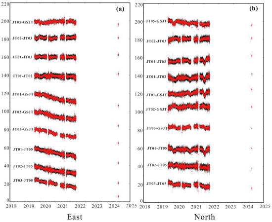
Figure 2.
Time series of GNSS short-baseline horizontal vectors. (a) Eastward horizontal baseline vector; (b) northward horizontal baseline vector.
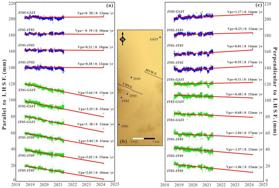
Figure 3.
Baseline component variation time series for the Laohushan Fault; (a) time series of baseline changes parallel to the Laohushan Fault, where Vpa represents the variation rate of the baseline component parallel to the fault; (b) distribution of GNSS stations; (c) time series of baseline changes perpendicular to the Laohushan Fault, where Vpe represents the variation rate of the baseline component perpendicular to the fault. Green points represent the baseline time series across the fault. Blue points represent the baseline time series on the same side of the fault. Red solid lines represent the linear rate of best fit from the least-squares method.
2.2.2. Regional GNSS Horizontal Velocity Field
The GAMIT/GLOBK software suite [36,37] was used to process double-differenced carrier phase observations (Figure 1), and daily loosely constrained solutions were obtained. A dual-frequency ionosphere-free combination was employed to mitigate first-order ionospheric effects, while higher-order ionospheric effects were corrected using the 2 h interval Total Electron Content (TEC) IONEX products provided by the Center for Orbit Determination in Europe (CODE). The geophysical models and parameters applied in the processing, such as the FES2004 tidal loading model, the GPT2 global pressure and temperature model, and the VMF1 mapping function, were consistent with those used by [35].
Instead of incorporating global daily solutions provided by the IGS analysis centers, we processed GNSS observation data from 70 core ITRF reference stations globally using the GAMIT package with identical modeling parameters. Daily coordinates and associated uncertainties were estimated by constraining the daily regional solutions with global solutions, and the daily free network solutions were transformed into the ITRF2014 reference frame [40] using the GLOBK package [37]. For campaign GNSS sites, linear velocities relative to ITRF2014 were computed using a weighted least-squares adjustment. Finally, the GNSS horizontal velocity field was transformed into the Eurasian reference frame using the Euler rotation vector for the Eurasian plate provided by [40], as illustrated in Figure 4.
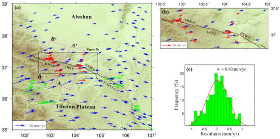
Figure 4.
GNSS horizontal velocity field of the Laohushan Fault and surrounding area (relative to the Eurasian reference frame); (a) the pink box indicates the location of the GNSS profile shown in Figure 5; (b) an enlarged view showing the denser GNSS velocity field around the Maomaoshan Fault and Laohushan Fault; (c) the errors associated with common points used in the 200 integration of the published velocity field.
To accurately analyze differential crustal motion between tectonic blocks, we utilized a GNSS velocity field referenced to the stable Eurasian plate [41]. In addition, to precisely model the tectonic characteristics of the Laohushan Fault and enhance our understanding of regional crustal horizontal deformation, we incorporated published high-density GNSS results [42,43], as indicated by the green arrows in Figure 4a. The Helmert parameter transformation method was employed to integrate these published results with the GNSS velocity field derived in this study, ensuring that the residual error at common points in the merged dataset was less than 1 mm/yr (Figure 4c).
3. GNSS Baseline Time Series
Using the GNSS baseline component time series (Figure 3), we applied the least-squares method to fit the rates of change for the baseline components both parallel and perpendicular to the Laohushan Fault. In this analysis, the southernmost station of each baseline served as the reference point, with other stations considered positive if they moved left relative to the reference point and negative if they moved right (as depicted in Figure 3 and Table 1). The results indicate that the baseline components parallel to the Laohushan Fault consistently exhibit a left-lateral strike–slip motion, while the components perpendicular to the fault primarily indicate relatively weak compressional shortening.

Table 1.
Fault-parallel and fault-perpendicular movement rates and associated error estimates derived from linear least-squares fitting.
Notably, all baselines crossing the Laohushan Fault (JT03-JT05, JT02-JT05, JT01-JT05, JT03-GSJT, JT02-GSJT, and JT01-GSJT) display significant variations in fitted parallel fault slip rates (>2.8 mm/yr). Specifically, within a narrow span of approximately 5 km across the fault (JT03-JT05), a left-lateral strike–slip rate of 2.81 ± 0.10 mm/yr is observed (Figure 2), accounting for 77% of the slip rate revealed by the longest baseline, JT01-GSJT (approximately 30 km), which measures 3.64 ± 0.13 mm/yr. In contrast, the baselines on the same side of the fault (not crossing the Laohushan Fault) (JT01-JT02, JT01-JT03, JT02-JT03, and JT05-GSJT) show minimal variation in their fitted parallel fault slip rates (<0.6 mm/yr) (Table 1). These deformation characteristics collectively suggest that within a 30 km span across the Laohushan Fault, nearly all strike–slip shear deformation is concentrated within a narrow zone of less than 3 km on either side of the fault, with the differential strike–slip motion across the fault inducing negligible deformation on the same side of the fault.
Additionally, the least-squares analysis of GNSS horizontal movement rates perpendicular to the fault strike reveals a degree of horizontal extensional deformation (0.5–1.2 mm/yr) on the same side of the fault (Table 1). Conversely, across the fault, there is consistent but relatively minor horizontal compressional deformation (−0.4 to −1.9 mm/yr) (Figure 3b). These findings suggest that neglecting deformation perpendicular to the fault could introduce uncertainties in accurately estimating the kinematic parameters of the Laohushan Fault’s creeping motion when using InSAR data.
4. GNSS Profiles and Inversions
The third section of this paper explores the strain distribution characteristics in the near-field region (within approximately 15 km on either side) of the Laohushan Fault, as revealed by the GNSS short-baseline fault motion components. The analysis identifies significant left-lateral creep along the Laohushan Fault. To further elucidate the detailed variations in strain distribution across both the near- and far-field regions of the fault, and to enhance our understanding of the constraints on fault movement characteristics at different depths, this study utilizes the regional GNSS horizontal velocity field. This field, which includes GNSS creep observation sites along the Laohushan Fault, was used to construct the GNSS velocity profile A–A’ across the fault (Figure 4b).
For a comparative analysis of the transverse differences in interseismic fault motion within the region, an additional GNSS velocity profile, B–B’, was constructed across the Maomaoshan Fault, located approximately 100 km west of the Laohushan Fault, using dense GNSS data along the Maomaoshan Fault (Figure 4b). The GNSS horizontal velocity components within the scope of these profiles were projected along directions parallel and perpendicular to the strikes of the Laohushan Fault (NE102°) and the Maomaoshan Fault (NE103°), respectively, to generate the GNSS velocity profiles for these two faults (Figure 5). A two-dimensional dislocation model incorporating fault creep motion was subsequently employed to invert and determine the geometric parameters (creep depth/locking depth) and kinematic parameters (creep rate/deep loading rate) associated with fault creep and locking.
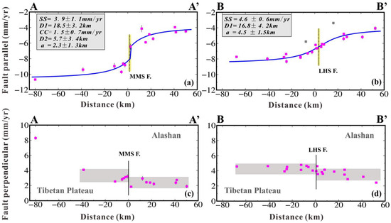
Figure 5.
(a,b) display the GNSS velocity components parallel to the fault, with pink squares indicating the data and gray squares representing outliers (which were not used in the inversion). (c,d) show the GNSS velocity components perpendicular to the fault, with similar color coding: pink squares for data and gray squares for outliers. The black dashed lines in (a–d) indicate the position of the fault as determined by inversion, with yellow shading representing the error margin. The 0 km mark denotes the actual fault position. The blue solid lines in (a,b) represent the inverse tangent curves calculated from the fault slip model, where SS denotes the slip rate, D1 indicates the locking depth, CC represents the shallow creep rate, and D2 denotes the creep depth. The gray shading in (c,d) represents the differential motion perpendicular to the fault on both sides. The black solid line shows the actual fault position.
4.1. Methods and Solution
We assume that plate motion occurs along one or more nearly vertical (upright) strike–slip faults, which are either locked or creeping from the surface to a certain depth. We use a combination of screw dislocation models [44,45,46,47,48] to perform inversion calculations for the Laohushan Fault and the Maomaoshan Fault. This model can simultaneously fit the deformation signals caused by both fault creep and deep locking, which represent two different physical mechanisms. The mathematical expression for this model can be described as follows:
represents the velocity parallel to the fault, represents the distance perpendicular to the fault, and represent the deep slip rate and locking depth of the fault, respectively, and represent the shallow creep rate along the fault strike and the creep depth, respectively, is the Heaviside step function, and represents the offset between the data and the model. In the actual inversion process, reasonable constraint ranges for the parameters to be estimated were provided based on previous research results [23,24,25,42]: 0 < < 20 mm/yr, 0 < < 20 km, 0 < < 10 mm/yr, and 0 < < 10 km, −20 < < 20 km. These parameters were assumed to follow a uniform prior distribution within the specified ranges, with an additional constraint < . After eliminating some obvious outliers and results with large errors (Figure 5), we used the Levenberg–Marquardt (L-M) method to linearize the nonlinear equations through a Taylor series expansion. The best-fit values and uncertainties for the parameters in the model were then determined through iterative calculations (Figure 5).
4.2. Results of GNSS Profile Inversion
The inversion results show (Figure 5a) that the Laohushan Fault currently exhibits a coupled motion characteristic with shallow creep and deep locking (the fault is not fully open). Specifically, the shallow left-lateral creeping rate is 1.5 ± 0.7 mm/yr, with a creep depth of 5.7 ± 3.4 km. The left-lateral elastic loading rate due to deep tectonic loading is 3.9 ± 1.1 mm/yr, and the elastic locking depth ranges from 5.7 ± 3.4 km to 16.8 ± 3.2 km. In contrast, the same inversion model applied to the Maomaoshan Fault profile (Figure 5b) does not reveal evidence of shallow fault creep. The left-lateral slip rate for the Maomaoshan Fault is determined to be 4.6 ± 0.6 mm/yr, with a locking depth of 16.8 ± 4.2 km, indicating a higher degree of strain accumulation compared to the Laohushan Fault.
Additionally, the horizontal offsets, estimated as free parameters, are 2.3 ± 1.3 km for the Laohushan Fault and 4.5 ± 1.5 km for the Maomaoshan Fault. These offsets correspond closely with the geological fault baselines, providing indirect validation of the observational data and inversion results. Furthermore, the horizontal shortening/extension rates across the faults, inferred from differential motion, suggest varying degrees of crustal shortening at both the Laohushan and Maomaoshan faults, with magnitudes not exceeding 1 mm/yr (Figure 5c,d).
5. Discussion
5.1. Comparison with Existing InSAR Results
In calculating the fault creep rate using InSAR observations, the effects of regional vertical deformation and deformation perpendicular to the fault cannot be neglected [23,25,26]. To account for these effects, we collected precise leveling data for the region from 1970 to 2012. By applying the dynamic least-squares adjustment method [49], we mitigated systematic errors by incorporating the vertical motion rates from continuous GNSS stations as a priori information. This approach enabled us to derive the vertical crustal deformation field for the study area (Figure 6). As depicted in Figure 6, the Haiyuan region exhibits complex vertical deformation, with vertical displacement rates of 1–2 mm/yr observed near the eastern segment of the Laohushan Fault.
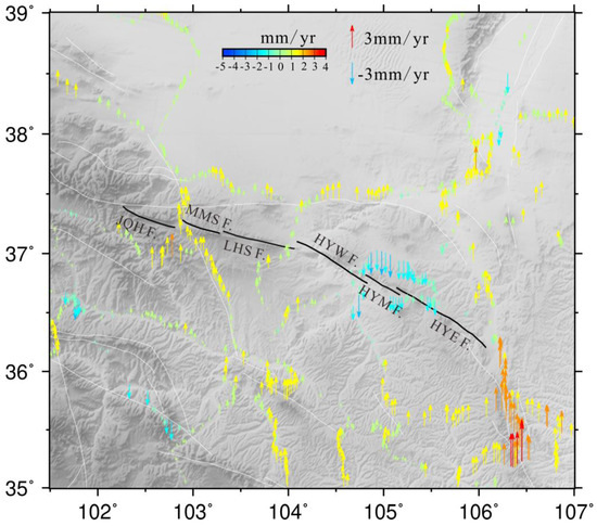
Figure 6.
Leveling vertical land motion rates in the Haiyuan Fault and its surrounding regions. Scale of the arrows indicates velocity magnitude, underlined by color. Positive (negative) values denote crustal uplift (subsidence).
We analyzed GNSS profiles and fault dislocation model inversion results for the Laohushan Fault (Figure 5) and found that its left-lateral creep occurs at shallow depths, above 5.7 ± 3.4 km, with a creep rate of 1.5 ± 0.7 mm/yr. These findings were compared with previously published estimates of the Laohushan Fault’s creep rate based on InSAR data (Table 2). As shown in Table 2, the GNSS-derived creep rate is lower than the values obtained using InSAR. Even within studies utilizing the same InSAR dataset (InSAR + GNSS (far-field)), discrepancies persist. Specifically, creep rates derived from combined ascending and descending InSAR observations [23,25,26] are lower than those obtained from single-track InSAR data [19,24].
Table 2.
Summary of creep rates along the Laohushan Fault Zone. (D: descending track InSAR observations; A/D: combined ascending and descending track InSAR observations).
When calculating fault deformation using InSAR technology, single-track InSAR observations require neglecting both vertical deformation and deformation perpendicular to the fault. In contrast, combined ascending and descending track InSAR data only necessitate ignoring deformation perpendicular to the fault [23,50,51]. Existing leveling observations (Figure 6) suggest a vertical deformation of 1–2 mm/yr near the eastern segment of the Laohushan Fault, while near-field GNSS continuous data from this study (Figure 3 and Figure 5) show 1 mm/yr of deformation perpendicular to the fault. In prior InSAR studies, whether using single-track or combined ascending and descending track observations, the inability to accurately separate vertical crustal deformation from fault-perpendicular deformation has likely led to overestimations of the creep rate of the Laohushan Fault. Therefore, to reliably calculate fault deformation characteristics from InSAR data, it is crucial to fully account for both vertical crustal deformation and deformation perpendicular to the fault.
5.2. Temporal and Spatial Variation in Creep Motion on the Laohushan Fault
Considering the lack of observations between June 2021 and March 2024 (Figure 2), and to avoid crustal deformation caused by seasonal changes, we selected observation data from the same season in different years. The slip rates for the two cross-fault GNSS baselines (JT03-JT05 and JT02-JT05) within the near-field of the Laohushan Fault (approximately 5 km) were calculated in segments (Figure 7a). The results show that the creep rate in the near-field of the fault does not exhibit significant changes over different time periods, indicating that the creep motion in the fault’s near-field is steady.
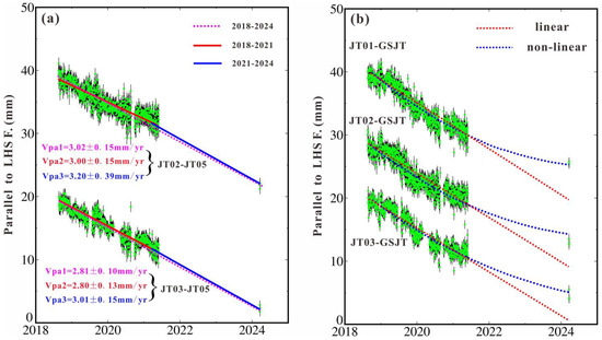
Figure 7.
(a) Rate fitting of the baseline component parallel to the fault in the near-field across the fault; (b) rate fitting of the baseline component parallel to the fault in the far-field across the fault. The red dashed line represents the least-squares linear fit, and the blue dashed line represents the result of the fitting using Equation (2).
In contrast, Figure 3a shows that the cross-fault baseline components parallel to the fault, composed of observation points farther from the fault (greater than 20 km), such as JT03-GSJT, JT02-GSJT, and JT01-GSJT, cannot be accurately fitted with a least-squares linear method for the final observation in 2024. There appears to be significant nonlinear deformation, and the discrepancies in the least-squares linear fit become more pronounced with longer baseline distances. Therefore, we attempt to fit the time series of these three parallel fault baseline components using a postseismic viscoelastic relaxation model (Equation (2)).
In this context, represents the baseline component parallel to the fault, denotes the epoch observation time, indicates the linear rate of change of the baseline component parallel to the fault, and represents a commonly used postseismic time series fitting function [52,53,54].
The fitting results presented in this paper (Figure 7b, blue dashed line) demonstrate that the postseismic relaxation model not only closely matches the continuous observations from 2018 to 2021 but also aligns well with the final observations in 2024. Notably, these nonlinear deformation features are absent in the fitting results of the baseline components perpendicular to the fault (Figure 3c). This suggests that if these effects are indeed related to postseismic relaxation from a nearby earthquake, the event in question was likely a left-lateral strike–slip earthquake.
In addition, the nonlinear deformation features observed in the far-field baselines parallel to the fault may be related to postseismic effects from the 1920 Haiyuan earthquake. To explore this possibility, we projected and decomposed the regional high-density GNSS velocity field obtained in this paper (Figure 3) along the direction parallel to the Haiyuan Fault (Figure 8). The results reveal a significant zone of rapid activity south of the 1920 Haiyuan earthquake rupture zone, overlapping with the far-field region of the Laohushan Fault. Additionally, GNSS velocity profiles (Figure 5) indicate that the fault-parallel component on the southern side of the Laohushan Fault is approximately 2 mm/yr faster than that of the Maomaoshan Fault. This observational analysis suggests that the far-field deformation of the Laohushan Fault is probably influenced by postseismic deformation from the 1920 Haiyuan earthquake.
On the other hand, baseline time series and dislocation model inversion results (Figure 3, Figure 5 and Figure 7) indicate that the near-field creep of the Laohushan Fault (within approximately 5 km) does not exhibit the postseismic exponential decay deformation pattern observed in the far-field long baselines. Instead, it shows a stable creep motion. Therefore, the stable shallow creep of the Laohushan Fault is unlikely to be significantly affected by the postseismic deformation of the 1920 Haiyuan earthquake.
5.3. Regional Fault Movement and Earthquake Hazard
Based on the GNSS profiles and dislocation model inversion results for the Laohushan Fault (Figure 5), the left-lateral creep is observed to occur at shallow depths above 5.7 ± 3.4 km, with a rate of 1.5 ± 0.7 mm/yr. This is comparable to the 2–3 mm/yr rate obtained from InSAR data, which accounts for vertical deformation effects [23,25]. Additionally, the results of this study do not support the claim by [22] that the Laohushan Fault is currently experiencing fully open creep, as also suggested by InSAR-based studies [24,42]. Instead, the Laohushan Fault is found to be locked within a depth range of 5.7 ± 3.4 to 18.5 ± 3.2 km (Figure 5).
The characteristics of shallow creep and deep locking observed on the Laohushan Fault are supported by regional seismic activity results [55]. Previous studies indicate that there have been almost no earthquakes of magnitude 3 or greater within the 0–5 km depth range of the Laohushan Fault, which is attributed to the presence of a loose, thick fault gouge in the shallow part of the fault [55]. The collected regional aftershock data from 2008 to 2019 also show that earthquakes of magnitude 3 or greater are primarily concentrated in the 5–20 km depth range of the Laohushan Fault (Figure 9b,c), which aligns closely with the deep fault locking layer position inferred in this study. Additionally, paleoseismic trench studies reveal that the Laohushan Fault has recorded more than two prehistoric earthquakes of magnitude 7.0 or greater since the Holocene [56]. Based on these findings, we conclude that the creep on the Laohushan Fault represents shallow fault activity, while the deep part of the fault is currently locked and experiencing significant strain accumulation, indicating that the fault’s potential for a strong earthquake warrants attention.
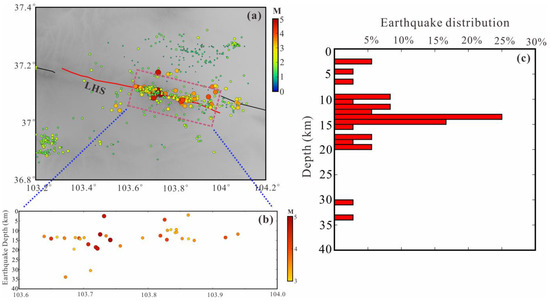
Figure 9.
The distribution of small earthquake activity on the Laohushan Fault: (a) The spatial distribution of small earthquake activity on the Laohushan Fault. (b) Red circles represent the projections of small earthquake activity along the depth of the Laohushan Fault, totaling 36 events. (c) The statistical distribution of earthquakes of magnitude 3 or greater with respect to the fault depth.

Figure 8.
GNSS velocity field parallel to the Haiyuan Fault. The colors in this Figure represent the magnitude of the velocity, while the direction of the arrows indicates the velocity direction. The red beach ball represents the focal mechanism solution [57].
Figure 8.
GNSS velocity field parallel to the Haiyuan Fault. The colors in this Figure represent the magnitude of the velocity, while the direction of the arrows indicates the velocity direction. The red beach ball represents the focal mechanism solution [57].

We compared the inversion results for the Laohushan and Maomaoshan Faults (Figure 4). The Maomaoshan Fault does not exhibit abrupt fault creep signals across the fault but rather shows typical interseismic locking characteristics. The inversion indicates a locking depth of 16.8 ± 4.2 km, which aligns with the 15 km estimate by [42]. The left-lateral slip rate of the Maomaoshan Fault, as determined in this study, is 4.6 ± 0.6 mm/yr, which is consistent with previous geological estimates [13,14,15,16,17,18] and geodetic estimates of 3 to 5 mm/yr [20,21,58]. Therefore, with its higher slip rate and locking depth, the Maomaoshan Fault currently poses a higher background risk for strong earthquakes.
It is worth noting that the results for the near-field baselines across the Laohushan Fault (approximately 5 km), JT03-JT05 and JT02-JT05 (Figure 3), show a left-lateral slip rate difference across the fault of 2.8–3.0 mm/yr. This is higher than the 1.5 ± 0.7 mm/yr creep rate estimated from the GNSS velocity profile (Figure 5b). This discrepancy may be due to the creep on the Laohushan Fault being concentrated in a smaller region on either side of the fault [23,25], which is smaller than the spacing of the existing GNSS near-field measurements. Therefore, future research should consider integrating dense GNSS and InSAR data to more accurately determine the creep parameters of the Laohushan Fault.
6. Conclusions
We used the latest densely spaced GNSS continuous observations across the Laohushan Fault and regional multi-source GNSS data as constraints to process and obtain precise baseline time series across the Laohushan Fault, as well as a densely monitored regional GNSS horizontal velocity field. The comprehensive analysis of these data reveals that the Laohushan Fault currently exhibits a left-lateral creep motion with characteristics of shallow creep and deep locking. The current fault creep mainly occurs in the shallow crust at depths of 0 to 5.8 ± 3.4 km at a rate of 1.5 ± 0.7 mm/yr. Below the creeping layer, down to a depth range of 16.8 ± 4.2 km, the fault is in a locked state with a locking rate of 3.9 ± 1.1 mm/yr. Additionally, the near-field creep motion (approximately 5 km) of the Laohushan Fault appears stable and seems unaffected by the postseismic effects of historical strong earthquakes in the adjacent area. However, the deep (far-field) tectonic deformation of the Laohushan Fault may be influenced by the postseismic effects of the 1920 Haiyuan M8.5 earthquake.
Author Contributions
Conceptualization, W.Z.; methodology, Y.L.; software, W.Z. and M.H.; validation, W.Z.; formal analysis, W.Z. and Y.L.; investigation, W.Z., S.S., M.H., B.L. and L.F.; data curation, W.Z.; writing, W.Z. and Y.L.; visualization, W.Z.; supervision, M.H. All authors have read and agreed to the published version of the manuscript.
Funding
This work was supported by the National Science Foundation of China (No. 42072243), the Science for Earthquake Resilience (No. XH24059YA), the Natural Science Basic Research Program of Shaanxi (program No. 2023-JC-QN-0309; program No. 2024JC-YBQN-0313), the National Natural Science Foundation of China (No. 12203060), and the Youth Innovation Promotion Association CAS (grant No. 2023426).
Data Availability Statement
All the processed data, models, and computing programs that support the findings of this study are available from the corresponding author upon request.
Acknowledgments
The Figures in this paper are made by GMT tools. We thank the editor, assistant editor, and anonymous reviewers for their constructive comments that improved the manuscript. The authors thank all the staff who participated in the GNSS surveys. We are grateful to the Crustal Movement Observation Network of China and the National Geodetic Control Network of China for providing part of the GNSS data.
Conflicts of Interest
The authors declare no conflicts of interest.
References
- Burgmann, R.; Schmidt, D.; Nadeau, R.M.; d’Alessio, M.; Fielding, E.; Manaker, D.; Murray, M.H. Earthquake potential along the northern Hayward fault, California. Science 2000, 289, 1178–1182. [Google Scholar] [CrossRef]
- Ryder, I.; Burgmann, R. Spatial variations in slip deficit on the central San Andreas Fault from InSAR. Geophys. J. Int. 2008, 175, 837–852. [Google Scholar] [CrossRef]
- Cattin, R.; Avouac, J.P. Modeling mountain building and the seismic cycle in the Himalaya of Nepal. J. Geophys. Res. Solid Earth 2000, 105, 13389–13407. [Google Scholar] [CrossRef]
- Barbot, S.; Lapusta, N.; Avouac, J.P. Under the hood of the earthquake machine: Toward predictive modeling of the seismiccycle. Science 2012, 336, 707–710. [Google Scholar] [CrossRef] [PubMed]
- Scholz, C.H. Earthquakes and friction laws. Nature 1998, 391, 37–42. [Google Scholar] [CrossRef]
- Kaneko, Y.; Avouac, J.P.; Lapusta, N. Towards inferring earthquake patterns from geodetic observations of interseismic coupling. Nat. Geosci. 2010, 3, 363–369. [Google Scholar] [CrossRef]
- Jolivet, R.; Candela, T.; Lasserre, C.; Renard, F.; Klinger, Y.; Doin, M.P. The burst-like behavior of aseismic slip on a rough fault: The creeping section of the Haiyuan fault, China. Bull. Seismol. Soc. Am. 2015, 105, 480–488. [Google Scholar] [CrossRef]
- Lohman, R.B.; McGuire, J.J. Earthquake swarms driven by aseismic creep in the Salton Trough, California. J. Geophys. Res. 2007, 112, B04405. [Google Scholar] [CrossRef]
- Zhang, J.; Wen, X.Z.; Cao, J.L.; Yan, W.; Yang, Y.L.; Su, Q. Surface creep and slip-behavior segmentation along the northwestern Xianshuihe fault zone of southwestern China determined from decades of fault-crossing short-baseline and short-level surveys. Tectonophysics 2018, 722, 356–372. [Google Scholar] [CrossRef]
- Lisowski, M.; Prescott, W.H. Short-range distance measurements along the San Andreas fault system in central California, 1975 to 1979. Bull. Seismol. Soc. Am. 1981, 71, 1607–1624. [Google Scholar] [CrossRef]
- Ambraseys, N.N. Some characteristic features of the Anatolian fault zone. Tectonophysics 1970, 9, 143–165. [Google Scholar] [CrossRef]
- Cakir, Z.; Akoglu, A.M.; Belabbes, S.; Ergintav, S.; Meghraoui, M. Creeping along the Ismetpasa section of the North Anatolian fault (Western Turkey): Rate and extent from InSAR. Earth Planet. Sci. Lett. 2005, 238, 225–234. [Google Scholar] [CrossRef]
- Ohzono, M.; Sagiya, T.; Hirahara, K.; Hashimoto, M.; Takeuchi, A.; Hoso, Y.; Wada, Y.; Onoue, K.; Ohya, F. Doke Strain accumulation process around the Atotsugawa fault system in the Niigata-Kobe Tectonic Zone, central Japan. Geophys. J. Int. 2011, 184, 977–990. [Google Scholar] [CrossRef]
- Anderlini, L.; Serpelloni, E.; Belardinelli, M.E. Creep and locking of a low-angle normal fault: Insights from the Altotiberina fault in the northern Apennines (Italy). Geophys. Res. Lett. 2016, 43, 4321–4329. [Google Scholar] [CrossRef]
- Hamiel, Y.; Piatibratova, O.; Mizrahi, Y. Creep along the northern Jordan Valley section of the Dead Sea Fault. Geophys. Res. Lett. 2016, 43, 2494–2501. [Google Scholar] [CrossRef]
- Li, C.; Zhang, P.Z.; Yin, J.; Min, W. Late Quaternary left-lateral slip rate of the Haiyuan fault, northeastern margin of the Tibetan Plateau. Tectonics 2009, 28. [Google Scholar] [CrossRef]
- Liu-Zeng, J.; Shao, Y.; Klinger, Y.; Xie, K.; Yuan, D.; Lei, Z. Variability in magnitude of paleoearthquakes revealed by trenching and historical records, along the Haiyuan Fault, China. J. Geophys. Res. Solid Earth 2015, 120, 8304–8333. [Google Scholar] [CrossRef]
- Shao, Y.; Liu-Zeng, J.; Van der Woerd, J.; Klinger, Y.; Oskin, M.E.; Zhang, J.; Yao, W. Late Pleistocene slip rate of the central Haiyuan fault constrained from optically stimulated luminescence, 14C, and cosmogenic isotope dating and high-resolution topography. GSA Bull. 2021, 133, 1347–1369. [Google Scholar] [CrossRef]
- Jolivet, R.; Lasserre, C.; Doin, M.P.; Guillaso, S.; Peltzer, G.; Dailu, R.; Sun, Z.-K.; Shen, X.X. Shallow creep on the Haiyuan fault (Gansu, China) revealed by SAR interferometry. J. Geophys. Res. Solid Earth 2012, 117, B06401. [Google Scholar] [CrossRef]
- Gan, W.; Zhang, P.; Shen, Z.K.; Niu, Z.; Wang, M.; Wan, Y.; Cheng, J. Present-day crustal motion within the Tibetan Plateau inferred from GPS measurements. J. Geophys. Res. Solid Earth 2007, 112, B08416. [Google Scholar] [CrossRef]
- Li, Y.; Liu, M.; Wang, Q.; Cui, D. Present-day crustal deformation and strain transfer in northeastern Tibetan Plateau. Earth Planet. Sci. Lett. 2018, 487, 179–189. [Google Scholar] [CrossRef]
- Jolivet, R.; Lasserre, C.; Doin, M.P.; Peltzer, G.; Avouac, J.P.; Sun, J.; Dailu, R. Spatio-temporal evolution of aseismic slip along the Haiyuan fault, China: Implications for fault frictional properties. Earth Planet. Sci. Lett. 2013, 377, 23–33. [Google Scholar] [CrossRef]
- Li, Y.; Nocquet, J.M.; Shan, X.; Song, X. Geodetic observations of shallow creep on the Laohushan-Haiyuan fault, northeastern Tibet. J. Geophys. Res. Solid Earth 2021, 126, e2020JB021576. [Google Scholar] [CrossRef]
- Qiao, X.; Qu, C.; Shan, X.; Zhao, D.; Liu, L. Interseismic slip and coupling along the Haiyuan fault zone constrained by InSAR and GPS measurements. Remote Sens. 2021, 13, 3333. [Google Scholar] [CrossRef]
- Huang, Z.; Zhou, Y.; Qiao, X.; Zhang, P.; Cheng, X. Kinematics of the ∼1000 km Haiyuan fault system in northeastern Tibet from high-resolution Sentinel-1 InSAR velocities: Fault architecture, slip rates, and partitioning. Earth Planet. Sci. Lett. 2022, 583, 117450. [Google Scholar] [CrossRef]
- Guo, N.; Wu, Y.; Su, G. Analysis of the fault slip, creep, and coupling characteristics of the Maomaoshan-Laohushan-Haiyuan Fault using InSAR and GNSS measurements. Tectonophysics 2023, 863, 229988. [Google Scholar] [CrossRef]
- Hao, M.; Wang, Q.; Shen, Z.; Cui, D.; Ji, L.; Li, Y.; Qin, S. Present day crustal vertical movement inferred from precise leveling data in eastern margin of Tibetan Plateau. Tectonophysics 2014, 632, 281–292. [Google Scholar] [CrossRef]
- Xu, X.; Tong, X.; Sandwell, D.T.; Milliner, C.W.; Dolan, J.F.; Hollingsworth, J.; Ayoub, F. Refining the shallow slip deficit. Geophys. J. Int. 2016, 204, 1867–1886. [Google Scholar] [CrossRef]
- Marchandon, M.; Hollingsworth, J.; Radiguet, M. Origin of the shallow slip deficit on a strike slip fault: Influence of elastic structure, topography, data coverage, and noise. Earth Planet. Sci. Lett. 2021, 554, 116696. [Google Scholar] [CrossRef]
- Wu, X.; Xu, X.; Yu, G.; Ren, J.; Yang, X.; Chen, G.; Hao, H. The China Active Faults Database (CAFD) and its web system. Earth Syst. Sci. Data 2024, 16, 3391–3417. [Google Scholar] [CrossRef]
- Pang, Y.J.; Zhang, H.; Cheng, H.H.; Dong, P.Y.; Wang, J.J.; Shi, Y.L. Three-dimensional numerical simulation of pull-apart basins: An example of the Laolongwan basin in the Haiyuan fault zone. Chin. J. Geophys. 2015, 58, 3615–3626. [Google Scholar] [CrossRef]
- Song, Z.; Zhang, G.; Liu, J.; Yin, J.; Xue, Y.; Song, X. Disaster Information Catalog of Global Earthquakes (9999 B.C. to 2010 A.D.); Seismological Press: Beijing, China, 2011; (In Chinese with English Preface). [Google Scholar]
- Wang, M.; Shen, Z.K.; Gan, W.J.; Liao, H.; Li, T.; Ren, J.; Qiao, X.; Wang, Q.; Yang, Y.; Li, P.; et al. GPS Continuous Monitoring of Dynamic Evolution of Deformation Field of Xianshuihe Fault. Sci. China Ser. D 2008, 38, 575–581. [Google Scholar]
- Huang, L.R.; Fu, Y. Analysis on the noises from continuously monitoring GPS sites. Acta Seismol. Sin. 2007, 20, 197–202. [Google Scholar] [CrossRef]
- Hao, M.; Li, Y.; Wang, Q.; Zhuang, W.; Qu, W. Present-day crustal deformation within the western Qinling Mountains and its kinematic implications. Surv. Geophys. 2021, 42, 1–19. [Google Scholar] [CrossRef]
- Herring, T.A.; King, R.W.; McClusky, S.C. GAMIT Reference Manual, GNSS Analysis at MIT, Release 10.6; Massachusetts Institute of Technology: Cambridge, MA, USA, 2015. [Google Scholar]
- Herring, T.A.; King, R.W.; McClusky, S.C. GAMIT Reference Manual, Global Kalman Filter VLBI and GNSS Analysis Program, Release 10.6; Massachusetts Institute of Technology: Cambridge, MA, USA, 2015. [Google Scholar]
- Petit, G. IERS Conventions (2010); U.S. Naval Observatory Observatoire de Paris: Paris, France, 2010. [Google Scholar]
- Lyard, F.; Lefevre, F.; Letellier, T.; Francis, O. Modelling the global ocean tides: Modern insights from FES2004. Ocean. Dyn. 2006, 56, 394–415. [Google Scholar] [CrossRef]
- Altamimi, Z.; Métivier, L.; Rebischung, P.; Rouby, H.; Collilieux, X. ITRF2014 plate motion model. Geophys. J. Int. 2017, 209, 1906–1912. [Google Scholar] [CrossRef]
- Wang, M.; Shen, Z.K. Present-day crustal deformation of continental China derived from GPS and its tectonic implications. J. Geophys. Res. Solid Earth 2020, 125, e2019JB018774. [Google Scholar] [CrossRef]
- Li, Y.; Shan, X.; Qu, C.; Zhang, Y.; Song, X.; Jiang, Y.; Wang, C. Elastic block and strain modeling of GPS data around the Haiyuan-Liupanshan fault, northeastern Tibetan Plateau. J. Asian Earth Sci. 2017, 150, 87–97. [Google Scholar] [CrossRef]
- Zhuang, W.; Cui, D.; Hao, M.; Song, S.; Li, Z. Geodetic constraints on contemporary three-dimensional crustal deformation in the Laji Shan–Jishi Shan tectonic belt. Geod. Geodyn. 2023, 14, 589–596. [Google Scholar] [CrossRef]
- Fattahi, H.; Amelung, F. InSAR observations of strain accumulation and fault creep along the Chaman Fault system, Pakistan and Afghanistan. Geophys. Res. Lett. 2016, 43, 8399–8406. [Google Scholar] [CrossRef]
- Savage, J.C.; Burford, R.O. Geodetic determination of relative plate motion in central California. J. Geophys. Res. 1973, 78, 832–845. [Google Scholar] [CrossRef]
- Savage, J.C. A dislocation model of strain accumulation and release at a subduction zone. J. Geophys. Res. Solid Earth 1983, 88, 4984–4996. [Google Scholar] [CrossRef]
- Savage, J.C. Viscoelastic-coupling model for the earthquake cycle driven from below. J. Geophys. Res. Solid Earth 2000, 105, 25525–25532. [Google Scholar] [CrossRef]
- Harris, R.A. Large earthquakes and creeping faults. Rev. Geophys. 2017, 55, 169–198. [Google Scholar] [CrossRef]
- Li, Z.; Hao, M.; Hammond, W.C.; Cheng, F.; Zhang, G.; Wang, Q.; Liu, L.; Hou, B.; Gan, W. Geodetic constraints on three-component motion of the Ordos block (China) and their implications for lithospheric dynamics. Geol. Soc. Am. Bull. 2024. [Google Scholar] [CrossRef]
- Liu, C.; Ji, L.; Zhu, L.; Xu, C.; Qiu, J. Interseismic strain rate distribution model of the Altyn Tagh Fault constrained by InSAR and GPS. Earth Planet. Sci. Lett. 2024, 642, 118884. [Google Scholar] [CrossRef]
- Hao, M.; Wang, Q.L.; Cui, D.X.; Liu, L.W.; Zhou, L. Present-day crustal vertical motion around the Ordos block constrained by precise leveling and GNSS data. Surv. Geophys. 2016, 37, 923–936. [Google Scholar] [CrossRef]
- Marone, C.J.; Scholtz, C.H.; Bilham, R. On the mechanics of earthquake afterslip. J. Geophys. Res. Solid Earth 1991, 96, 8441–8452. [Google Scholar] [CrossRef]
- Tian, Z.; Freymueller, J.T.; Yang, Z. Postseismic Deformation due to the 2012 Mw 7.8 Haida Gwaii and 2013 Mw 7.5 Craig Earthquakes and its Implications for Regional Rheological Structure. J. Geophys. Res. Solid Earth 2021, 126, e2020JB020197. [Google Scholar] [CrossRef]
- Tian, Z.; Freymueller, J.T.; Yang, Z.; Li, Z.; Sun, H. Frictional Properties and Rheological Structure at the Ecuadorian Subduction Zone Revealed by the Postseismic Deformation Due to the 2016 Mw 7.8 Pedernales (Ecuador) Earthquake. J. Geophys. Res. Solid Earth 2023, 128, e2022JB025043. [Google Scholar] [CrossRef]
- Liu, B.Y.; Yin, Z.W.; Yuan, D.Y.; Li, L.; Wang, W. The research on fault plane solution and geometric meaning of the Laohushan fault in the northeastern Tibetan plateau. Seismol. Geol. 2023, 42, 1354–1369. [Google Scholar]
- Liu-Zeng, J.; Klinger, Y.; Xu, X.; Lasserre, C.; Chen, G.; Chen, W.; Zhang, B. Millennial recurrence of large earthquakes on the Haiyuan fault near Songshan, Gansu Province, China. Bull. Seismol. Soc. Am. 2007, 97, 14–34. [Google Scholar] [CrossRef]
- Li, Y.; Shan, X.; Gao, Z.; Qu, C. Interseismic Coupling–Based Stochastic Slip Modeling of the 1920 Ms 8.5 Haiyuan Earthquake. Seismol. Res. Lett. 2024, 95, 870–878. [Google Scholar] [CrossRef]
- Loveless, J.P.; Meade, B.J. Partitioning of localized and diffuse deformation in the Tibetan Plateau from joint inversions of geologic and geodetic observations. Earth Planet. Sci. Lett. 2011, 303, 11–24. [Google Scholar] [CrossRef]


Disclaimer/Publisher’s Note: The statements, opinions and data contained in all publications are solely those of the individual author(s) and contributor(s) and not of MDPI and/or the editor(s). MDPI and/or the editor(s) disclaim responsibility for any injury to people or property resulting from any ideas, methods, instructions or products referred to in the content. |
© 2024 by the authors. Licensee MDPI, Basel, Switzerland. This article is an open access article distributed under the terms and conditions of the Creative Commons Attribution (CC BY) license (https://creativecommons.org/licenses/by/4.0/).