Abstract
Melt ponds play a crucial role in the melting of Arctic sea ice. Studying the evolution of melt ponds is essential for understanding changes in Arctic sea ice. In this study, we used a revised sea ice model to simulate the evolution of melt ponds along the MOSAiC drift at a resolution of 10 m. A novel melt pond parameterization scheme simulates the movement of meltwater under the influence of gravity over a realistic sea ice topography. We evaluated different melt pond parameterization schemes based on remote sensing observations. The absolute deviation of the maximum pond coverage simulated by the new scheme is within 3%, while differences among parameterization schemes exceed 50%. Errors were found to be primarily due to the calculation of macroscopic meltwater loss, which is related to sea ice surface topography. Previous studies have indicated that sea ice with a lower surface roughness has a larger catchment area, resulting in larger pond coverage during the melt season. This study has identified an opposing mechanism: sea ice with lower surface roughness has a larger catchment area connected to the macroscopic flaws of the sea ice surface, which leads to more macroscopic drainage into the ocean and thereby a decrease in melt pond coverage. Experimental simulations showed that sea ice with 46% higher surface roughness, resulting in 12% less macroscopic drainage, exhibited a 38% higher maximum pond fraction. The presence of macroscopic flaws is related to the fragmentation of sea ice cover. As Arctic sea ice cover becomes increasingly fragmented and mobile, this mechanism will become more significant.
1. Introduction
The Earth’s climate is subject to continual changes, notably in the Arctic region, where the melting of snow and sea ice leads to the formation of melt ponds in summer [1]. These melt ponds, characterized by a lower albedo compared to the surrounding ice, contribute to the increased absorption of solar radiation. Recognizing the significance of this phenomenon, various studies have been conducted to integrate precise parameterizations of melt ponds into regional sea ice or global climate models, aiming to enhance the accuracy of sea ice forecasts [2,3,4]. Researchers have extensively investigated the dynamics of melt pond coverage on sea ice [5,6,7,8]. The evolution of pond coverage can be divided into different stages [9]. In the initial stage, the ponds experience rapid growth while the ice remains impermeable. Subsequently, as the ice transitions from impermeable to permeable, the ponds undergo a swift drainage process, resulting in a reduction in pond coverage. The pond water generally maintains the sea level until either the ponds refreeze or, in the event of an ice floe breakup, the ice disperses. Incorporating these insights into global climate models is imperative for improving the accuracy of sea ice forecasts and advancing our understanding of the impacts of climate change on polar regions.
Melt ponds are distributed in local topographic lows of the sea ice, with water volume being determined by the balance of inflow and outflow. Sea ice is a complex multiscale porous medium with diverse and multiscale pore structures and multiple permeability properties [9,10,11,12,13]. Outflow of meltwater can occur through vertical drainage through the interconnected pore structure within the ice or through horizontal movement of meltwater across the ice surface to macroscopic flaws, such as ice floe edges [1], cracks, and leads [9]. The simulation of the fluid flow behavior of sea ice has traditionally relied on sub-grid parameterization exemplified by approaches like the topo (topographic) [3] and lvl (level-ice formation) [14] schemes in the Los Alamos sea ice model version 6.3.1 (CICE6.3.1) [15] and the one-dimensional models outlined in the works of Eicken et al. (2002) [9], Taylor et al. (2004) [16], Lüthje et al. (2006) [17], and Skyllingstad et al. (2009) [18]. Lüthje et al. (2006) presented a model that initialized with the surface topographies of sea ice and studied the importance of the vertical seepage rate of melt pond evolution [17]. Popović et al. (2017) introduced a model for the evolution of melt pond coverage on permeable sea ice floes based on the assumption that the whole floe is in hydrostatic balance [19]. However, none of these models parameterized the horizontal drainage of meltwater across macroscopic flaws in the ice floe and simply provided a lenient and unsophisticated parameterization. The impact of different outflow pathways on melt pond evolution at different stages has not been compared. In this study, we indicate the dominant role of macroscopic outflow in the first stage of melt pond evolution, which determines an important parameter of sea ice variation, the maximum melt pond fraction (MPF), on the ice surface.
As Arctic sea ice becomes more fragmented during the melting season, meltwater runoff from the macroscopic flaws is expected to increase. However, the topic has received limited research attention. To address this gap, a new approach is proposed to enhance the understanding of meltwater budgets during the melting season. We leverage a G-D (Gradient Descent) algorithm to explicitly govern the horizontal movement of meltwater. The methodology begins by addressing vertical drainage through the application of Darcy’s Law, as elucidated by Eicken et al. (2002) [9]. Subsequently, any remaining meltwater, post-vertical drainage, is systematically redistributed horizontally to local topographic lows or macroscopic flaws of sea ice through iterations of the G-D algorithm. This model aims to simulate the dynamic evolution of melt ponds on individual ice floes. Using the model, we aim to (a) simulate the melt pond evolution on ice floes along the track of the Multidisciplinary drifting Observatory for the Study of Arctic Climate (MOSAiC) from 21 June to 2 August 2020, (b) compare the simulated MPF with remote sensing observations and the simulation results of the CICE6 schemes, and (c) study the relative importance of the two different outflow pathways (vertical drainage and runoff from the macroscopic flaws) in regard to the meltwater budget and their influence on the melt pond evolution. This research therefore contributes to a deeper understanding of the complex dynamics associated with melt pond evolution on ice floes, particularly in the context of the changing Arctic sea ice landscape.
2. Data
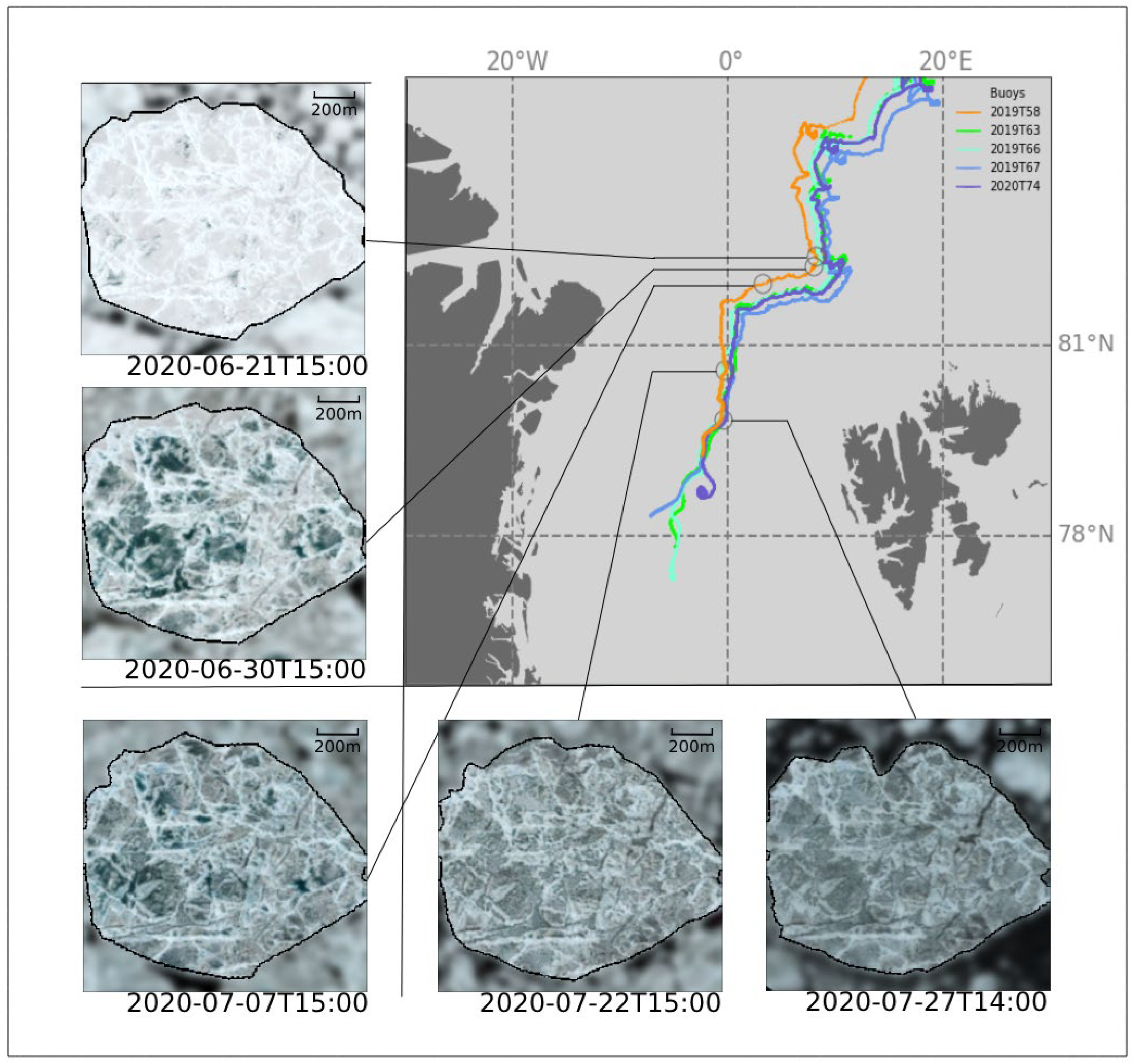
During the 2019–2020 period, the year-long MOSAiC Arctic research expedition aboard the research vessel (RV) Polarstern conducted comprehensive measurements and analyses of sea ice, ocean dynamics, atmospheric conditions, ecological phenomena, and bio-geochemical processes over the course of a complete seasonal rotation [20,21,22]. The melt pond evolution of ice floes during the MOSAiC campaign in summer 2020 was investigated using in situ measurements and optical satellite imagery [8,23,24]. During the MOSAiC campaign, Snow and Ice Mass Balance Array (SIMBA) buoys were deployed on ice floes in the Arctic Ocean over the distributed network (DN) and the central observatory [25]. Lei et al. (2021) processed the SIMBA measurements to derive snow depth and ice thickness [26]. The position information of the buoys was used to track and identify ice floe images. An example of the processing results is shown in Figure 1.
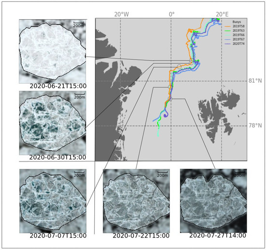
Figure 1.
Drift trajectories of five SIMBA buoys selected for simulation and Sentinel-2 images of the floe on which buoy 2019T58 was deployed.
To validate the modeling results of this study, we use remote sensing data and the partial shape recognition method to track, identify, and match cloudless (cloud percentage less than 10%) Sentinel-2 MSI satellite images of ice floes. The Hausdorff distance is used to measure the similarity of segmented ice floes. It is tolerant to perturbations and deficiencies in floe shapes [27]. The position information of the SIMBA buoys was used to track and identify ice floe images. Figure 1 illustrates the drift trajectories of five buoys selected for simulation and true-color Sentinel-2 MSI images showing an example floe over time. We retrieved cloud-free images of the ice floe throughout the melting season. Furthermore, we identified and matched the ice floe in the images and then used the LinearPolar algorithm to identify melt ponds on the processed satellite images of the ice floe; the algorithm treats melt ponds as features with variable albedo, and its error is approximately 30% lower compared to previous algorithms [28]. These images illustrate the various stages of melt pond evolution on the ice floe from its initial to final stages. As the true-color images in Figure 1 show as an example, ice floes were chosen with minimal shape changes during the 2020 melt season. This suggests that these ice floes experienced negligible deformation during the melt season. Therefore, we reproduced the evolution of these ice floes using a single-column sea ice model that does not include a dynamic scheme. This helps to simplify our model and make it more suitable for the study of the melt pond evolution process that we are concerned with.
The atmospheric forcing for the model includes the following: 2 m temperature, 2 m specific humidity, incoming long-wave radiation, incoming shortwave radiation, 2 m wind speed, and precipitation, which was further categorized into snow and rain. The forcing data were collected during the MOSAiC expedition and retrieved from the Atmospheric Radiation Measurement (ARM) User Facility (http://dx.doi.org/10.5439/1025153, accessed on 27 October 2022). The oceanic forcing field consist of SST, SSS, and zonal and meridional ocean velocities. The oceanic forcing data were obtained from CTD (Conductivity, Temperature, Depth) buoys during the MOSAiC Expedition [29]. The data were resampled to the time step of the model with linear interpolation. The simulated ice floe sizes were in the range of several kilometers, so the same value was used throughout the forcing field.
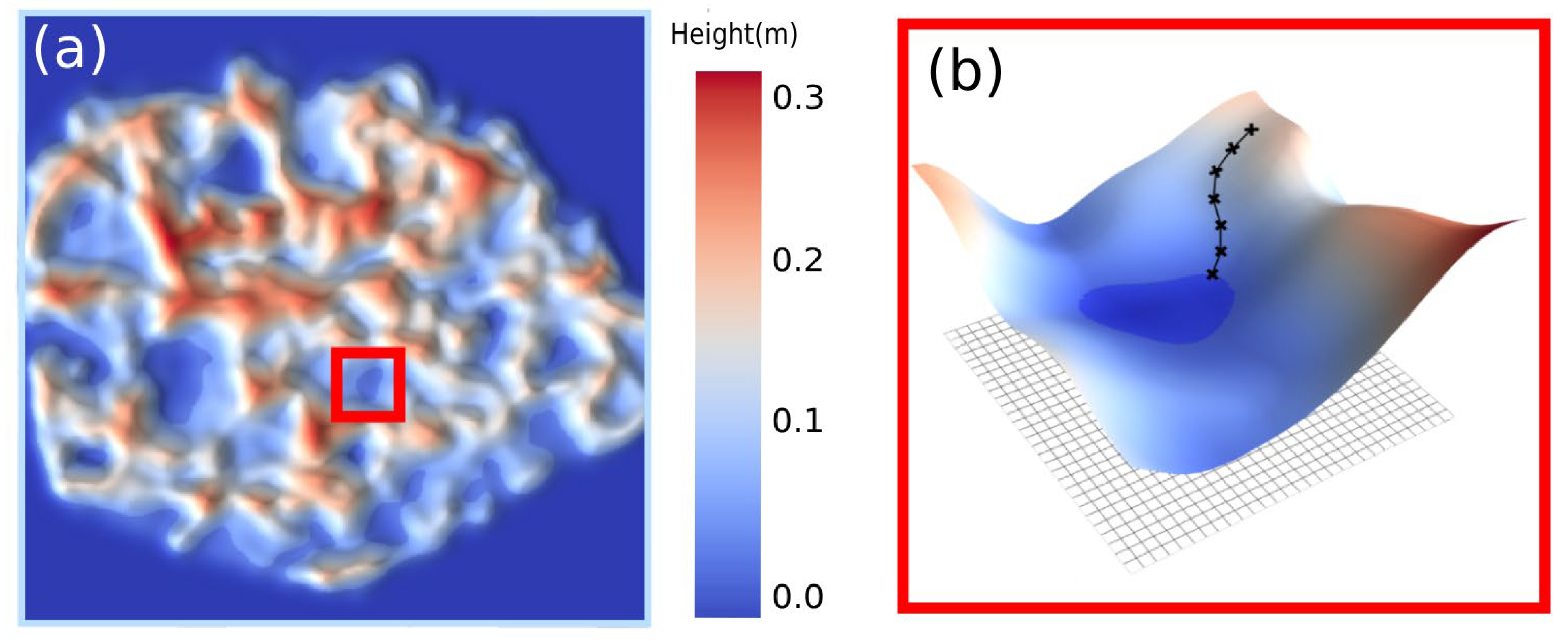
Sentinel-2 images of the ice floe were used to retrieve the depth of the snowdrift. Initial ice and snow topographies of the floes were generated from the depth of the snowdrift. We assumed the snow/ice interface to be flat, and any positive change in surface height is regarded as snowdrift. It should be noted that the uncertainty of this assumption remains to be verified [20]. The depth of the snowdrift is derived from ice surface reflectivity and ice surface temperature using Sentinel-2 remote sensing data, following the algorithm of Wang et al., 2023 [30]. An example of the topography of the observed floe is shown in Figure 2a.
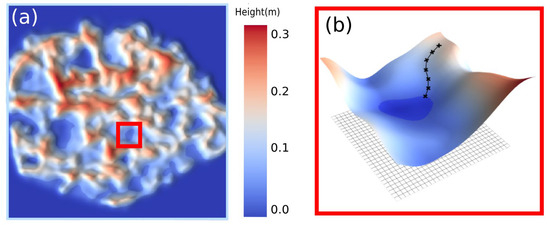
Figure 2.
Illustration of the proposed melt pond scheme. (a) Three-dimensional surface topography and melt ponds of the floe where SIMBA buoy 2019T58 was deployed. (b) A section of the sea ice surface marked by the red box in (a) and the pathway of meltwater acceleration at the topography low determined using G-D.
3. Methodology
This section begins with a description of the Icepack model, which forms the foundation of our simulations, including its key features and the specific configurations applied in our study. Following this, we introduce the melt pond evolution scheme developed for this research, highlighting its novel approach to meltwater distribution and drainage within the spatial grid framework.
3.1. Icepack Model
In this study, we utilized Icepack v1.3.1 [31], a single-column sea ice model in CICE 6. Icepack can be used as a stand-alone model; it simulates all vertical processes in CICE, including an ice thickness distribution scheme, thermodynamics module, solar radiation module, melt pond scheme, and ocean mixed-layer parameterization scheme. Sea ice in the Arctic contains a mixture of thin first-year ice, thicker multi-year ice, and thick pressure ridges. Therefore, in Icepack, snow and ice are represented in multiple layers and ice thickness is distributed into categories. In this study, we model an individual ice floe, so we use one ice thickness category, seven layers to represent ice, and three layers to represent snow or melt ponds. Icepack simulations were run with the mushy-layer thermodynamical model. This energy-conserving thermodynamical model treats the ice as a mushy layer [32], a matrix of pure ice that contains pockets of salty meltwater (brine). The model updates temperatures to compute melt and growth. This ensures that surface temperatures stay below 0 °C and bottom temperatures match the freezing point of water, with ice temperatures being calculated per layer via heat conduction. The multiple scattering radiative transfer scheme, the Delta-Eddington scheme, was used to account for solar radiation absorption, scattering, and transmittance of sea ice, including the effect of melt ponds [33]. Icepack includes an optional thermodynamic slab ocean mixed-layer parameterization, which is utilized when running the model without coupling to an ocean model. In all of our runs, the slab ocean parameterization was switched on.
Icepack offers three different schemes for modeling melt ponds: the CESM scheme, the topo scheme, and the lvl formulation. The CESM scheme describes melt pond processes empirically [14]. The topo scheme assumes that meltwater begins to accumulate from the areas with the minima elevation on the ice surface [3], while the lvl formulation restricts pond formation to areas of undeformed ice [14]. Both of these schemes consider a part of the characteristics of meltwater distribution under hydraulic control and therefore have disadvantages: the topo scheme does not allow for water surface elevation differences between melt ponds, while the lvl formula does not take into account the formation of melt ponds over areas of deforming ice. In all schemes, melt pond water can drain depending on ice permeability, but the meltwater runoff from the macroscopic flaws is parameterized using the tuning parameter and only depends on ice concentration rather than, e.g., ice surface roughness [4]. The area and volume of melt ponds were found to be highly sensitive to the tuning parameter choices [34]. This study used a new meltwater distribution scheme to provide a more detailed and explicit parameterization of the meltwater runoff from macroscopic flaws, which will be introduced in the next section.
3.2. Melt Pond Evolution Scheme
A spatial grid was created that was consistent with the Sentinel-2 ice floe images shown in Figure 1. We applied the column physics (Icepack) model to each grid cell, with neighboring cells being independent of each other unless the horizontal meltwater flow passes from one to another. As meltwater drainage occurs more rapidly in the vertical direction than in the horizontal direction, we first solved the vertical drainage for each computational time step by using Darcy’s Law and following the “mushy” thermodynamic option according to Turner and Hunke 2015 [34]. Liquid water, , is produced in a given grid cell by the melting of snow and ice and may be supplemented by liquid precipitation:
where and are ice and snow densities, and are the thicknesses of the ice and snow that melted, is the rainfall rate, is the fraction of the total meltwater available that is added to the ponds, is the total fractional ice area, and is the time step. Calculating meltwater flow through sea ice is highly complex and challenging. The meltwater flow through porous sea ice is described with Darcy’s Law:
where is gravitational acceleration, is the density of water, is the dynamic viscosity, is the total pressure drop, which is equal to the height difference between the sea ice surface and sea level, and is the vertical permeability of sea ice with units of length squared.
Considering the surface elevation as a function of coordinates , under the action of gravity, the remaining meltwater after vertical drainage at will be distributed to the local minima of in the vicinity of . If there is still meltwater left in the grid cell after vertical drainage, the remaining meltwater will be horizontally redistributed to the nearby topographic lows by applying the G-D iteration:
The iteration comes to an end when:
or
where is the topography as a function of the spatial coordinate , is the number of iterations, is the position of times iteration, and is the step of the iteration, representing the size of the change per iteration update, taken as . is a threshold of slope between position and , taken as . is the grid cells of ponded ice and is the open water grid cells. The meltwater of the grids gathers in a shared topographic low, forming a collective melt pond, as shown in Figure 2b, for an arbitrary section of the sea ice surface. The meltwater of the grid cells reaching the floe edge rather than a local topography low is drained into the ocean. The iteration step is important in determining whether the iteration will reach the local minima or the global minimum. It should be noted that, as a case study, the iteration step used here is arbitrary. The appropriateness of this value is related to the size of the melt ponds and the fluctuation degree of the ice surface elevation (ice surface roughness). A more representative value depends on more statistics on these sea ice morphological parameters, which will be compiled in the next work.
3.3. Model Setup
The experiments in this study were conducted in a single ice floe domain, assuming no deformation. Therefore, the dynamic module of the CICE model was switched off and only the Icepack was used. The model was run with a spatial resolution of 10 m, utilizing a Mercator projection, which matches the resolution of Sentinel-2 MSI images for comparison. The Icepack thermodynamic model was applied to each model grid to simulate the production of meltwater. Following this, a meltwater distribution scheme was applied to simulate meltwater flowing vertically and horizontally through the sea ice. The original scheme allows all three surface types (ice, snow, pond) to exist within the same ice thickness category. In the modified scheme, each grid cell can be in one of four potential states: bare ice, open water, snow-covered ice, and melt pond-covered ice. The shape of the ice floe was assumed to remain constant, so there is no transition between open water and the other three states; thus, the open water cell only exists as a mask. The grid cells of ponded ice were determined by the meltwater distribution scheme, and snow-covered ice can be converted to melt pond grid cells depending on the meltwater distribution scheme. Besides control runs, (Table 1) we designed experiments based on the topo and lvl meltwater schemes in Icepack. In the TOPO run, meltwater starts flooding from the lowest point of a floe, with all melt ponds maintaining a uniform surface height. In the LVL run, we confined the melt pond formation to flat ice areas, allowing for elevation differences between pond surfaces. To further investigate the differences in simulation accuracy between the schemes, we designed a TOPO-H run and LVL-H run where the macro-flaw outflow was added. In the TOPO-H run and LVL-H run, similar to the CNTL run, the meltwater from grid cells reaching the floe edge, rather than a local topographic low, is drained into the ocean. It should be note that these experiments do not directly assess the performance of the schemes in Icepack and CICE, as we utilized a modified high-resolution model. In our simulations, the grid scale is finer than the physical scale of meltwater flow, whereas the melt pond schemes in Icepack is a sub-grid parameterization. Specifically, the lvl scheme in Icepack calculates melt pond coverage based on a fixed ratio of melt pond depth to fraction, causing our LVL run to differ significantly from the Icepack scheme. The primary objective of these experiments is to assess the mechanistic assumptions underlying various melt pond schemes while minimizing the influence of errors related to ice topography determined by ice thickness distribution.

Table 1.
Settings for the control runs and experimental simulations. All of these cases were carried out for each of the five buoys.
All the runs were started from a fixed initial sea ice condition rather than a restart from a spin-up run. We ran the model from 21 June 2020, when melt ponds were not yet formed, using a realistic initial sea ice condition retrieved from remote sensing and the MOSAiC observations. The MOSAiC ice is described as multi-year ice or, more specifically, as second-year ice [23]. The limitation of running such a short simulation is the non-representation of multi-year ice. Since we used observational topography data to describe the deformation of multi-year ice, it is sufficient to set the initial sea ice condition instead of a restart from a spin-up. All simulations were initialized using the ice thickness, snow depth, and internal ice temperature (at locations corresponding to the center of the snow and ice layers) recorded by the SIMBA buoys while assuming that the entire ice floe has a uniform ice thickness, snow depth, and internal ice temperature profile. Experiments were also designed to study the effects of different ice surface topography on meltwater transport and the MPF (Table 1). All simulations utilized a time step of 1800 s. All model experiments in this study focused on the period from 21 June 2020 to 27 July 2020, for which extensive forcing data were available from the MOSAiC expedition, and optical remote sensing data could be used to verify the melt pond simulation results.
4. Results and Discussion
The present study employed a numerical model to simulate variations in the melt pond coverage of multiple sea ice floes along the MOSAiC observations during the melting season. Remote sensing observations of melt pond coverage served as the reference, while different experimental setups were tested to assess the modeling capability of various melt pond parameterization schemes. Different experimental setups are outlined in Table 1, with all other settings being kept consistent unless otherwise specified in the table. The remote sensing-based MPF was derived using the Sentinel-2 algorithm based on Wang (2020), which was validated to have an error of less than 4% [28]. Due to the limitation of cloud cover in visible remote sensing, MPF observations are not continuous daily results but scattered observations in five weather windows during the melt period (21 June, 30 June, 7 July, 27 July, and 21 July). These observation dates cover all stages of melt pond development and are therefore representative. The simulation experiments also included experiments with two different ice surface topographies to investigate the relationship between sea ice surface topography and melt pond coverage.
4.1. Gradient Descent Scheme
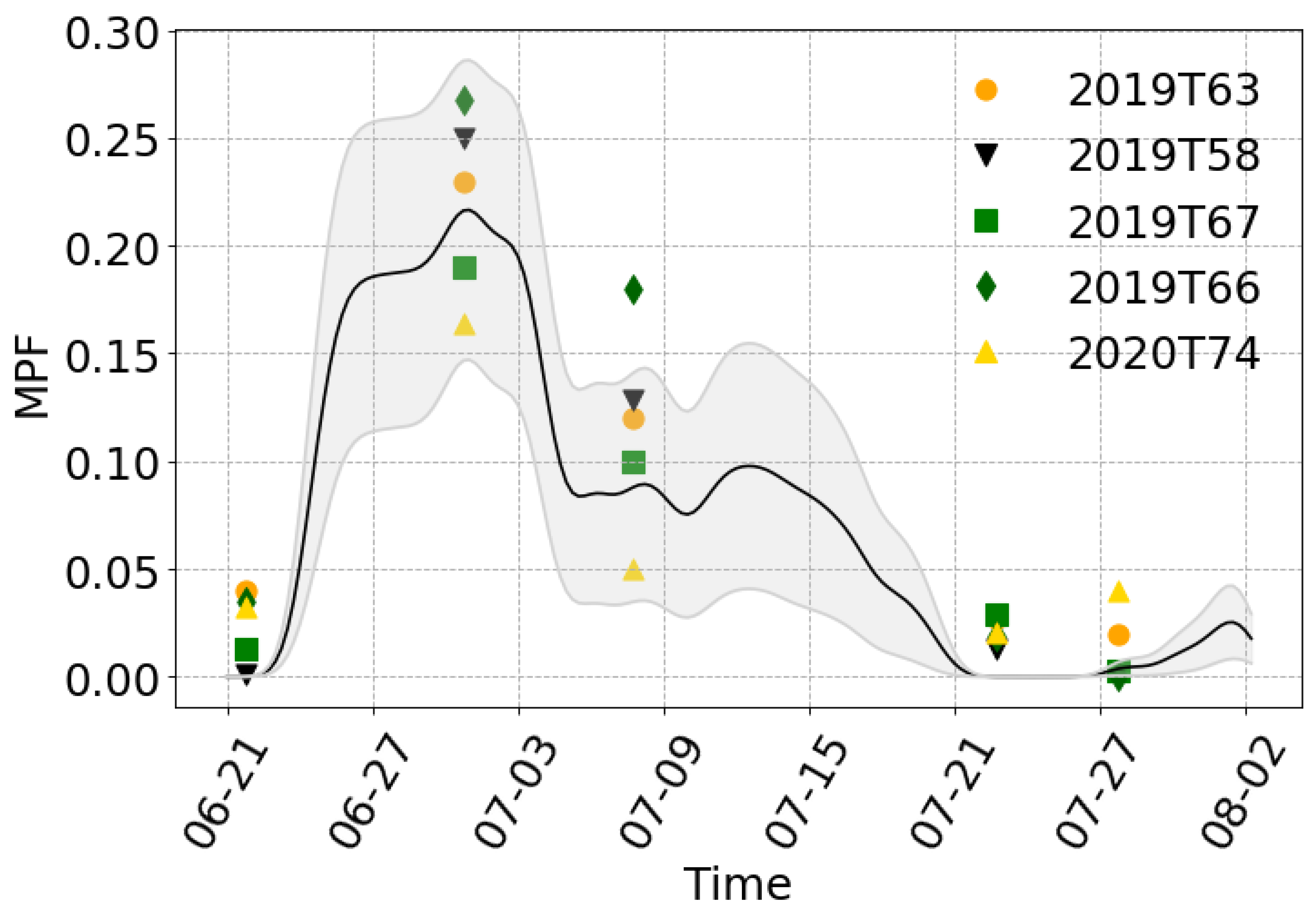
Figure 3 illustrates the seasonal evolution of the maximum MPF simulated using the G-D scheme (control run in Table 1). The simulated maximum MPF ranges from 15% to 28%, peaking at around 30 June. Initially, pond formation progresses rapidly, reaching the maximum fraction within a week, followed by a swift decline to half the maximum within another week. The MPF then stabilizes until mid-July, followed by a continuous decrease until disappearing around 21 July. The seasonal pond observations from Sentinel-2 data, also shown in Figure 3, exhibit a similar pattern, with the observed maximum MPF ranging from 16% to 27%, consistent with the simulation results. Notably, both observations and simulations demonstrate that the maximum MPF occurs around 30 June, aligning with high solar radiation input. Due to cloud cover over the ice surface, effective optical remote sensing observations are limited to clear-sky conditions. A large number of effective visible remote sensing observations coincide with the maximum or phasic peaks in MPF evolution, as ice under clear skies receives a significant amount of solar radiation input. Moreover, the floes were located close to each other throughout the melt season, so the same atmospheric and oceanic forcing was used. Therefore, the MPF evolution trends were similar in all cases.
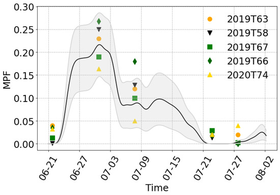
Figure 3.
Comparison of the MPF evolution between modeling and remote sensing. The line indicates the simulated mean MPF across the melting season of different floes, the shadow indicates the standard deviation of the simulated MPF of different floes, and the markers represent the MPF observed from Sentinel-2 images of different floes on different dates.
Figure 4 illustrates a comparison between the observed maximum MPF from Sentinel-2 imagery and the modeling results from the control run. The simulation results demonstrate a close agreement with the Sentinel-2 observations, with a Mean Absolute Error (MAE) of 0.022 and a Root Mean Square Error (RMSE) of 0.027. The modeled maximum MPF closely matches the observed values, with only a slight underestimation of around 3%. However, there is a systematic underestimation in the MPF during each stage of the simulation, particularly notable during the late stages of pond evolution. For instance, on 7 July, the mean MPF from observations is 0.088, while the mean MPF from the simulation is 0.12, representing an underestimation of 23%. During the other three remote sensing observation windows, the simulated pond coverage is either zero or close to zero, while the remote sensing observations indicate a pond coverage of below 4%. This systematic underestimation in the modeled MPF may be attributed to the spatial resolution (10 m) of the sea ice surface elevation data, which fails to represent small-scale pits, thereby preventing the model from simulating some small-sized ponds accurately.
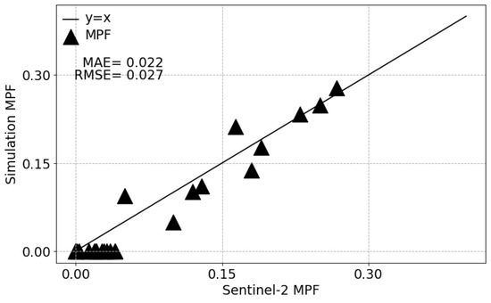
Figure 4.
Scatter plot of observed and simulated MPF of control run.
4.2. Comparison between Different Melt Pond Schemes
In the control run experiment, we simulated the development of MOSAiC melt ponds using a G-D scheme. The scheme simulated the hydraulic control of melt pond formation in realistic topography, including the parameterization of meltwater loss to macro-flaws. The simulation of the process in the CICE model with the topo and lvl schemes is simplified. One scheme assumes that meltwater begins to accumulate from the areas with the minima elevation on the ice surface while the other uniformly distributes meltwater across flat ice areas. Neither of these schemes parameterize the loss of meltwater flowing into macro-flaws, and the boundary between ice and open water is closed, preventing meltwater from draining through the ice edge. We designed experiments to discuss the potential impact of this on the accuracy of melt pond simulation. The effects of different schemes on melt pond simulation are shown in Figure 5a. Compared to observations, both the topo and lvl schemes overestimate the MPF in the early stages of melting, with overestimations of approximately 50% and 40%, respectively, for the maximum MPF. In the late stage, all three schemes underestimate the MPF, with topo underestimating it by 53% and CNTL and LVL underestimating it by around 38%.
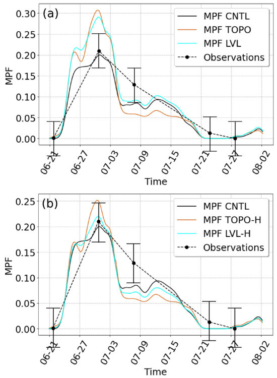
Figure 5.
Comparison of the MPF evolution. (a) Comparison between the observation and the CNTL, TOPO, and LVL runs. The black dots indicate the MPF observed from Sentinel-2 images. Lines indicate the simulated MPF. (b) Comparison between the observation and the CNTL, TOPO-H, and LVL-H runs. The black dots indicate the MPF observed from Sentinel-2 images. Lines indicate the simulated MPF. The error bars represent the error of the classification scheme. Note that the y-scales of (a,b) are not the same.
In the TOPO and LVL runs, the meltwater outflow from macro-flaws is excluded. As previously mentioned, there are two main differences between the G-D scheme and the topo and lvl schemes: differences in the parameterization of hydraulic control of pond formation and meltwater outflow from macro-flaws. As shown in Figure 5b, both the TOPO-H and LVL-H runs show significant improvements in early-stage pond simulations compared to the TOPO and LVL runs. The TOPO-H run overestimates the maximum pond coverage by 19%, while the LVL-H run overestimates it by only 4.3%, approaching the accuracy of CNTL. In the late melting stage, the results of the TOPO-H and LVL-H runs do not show significant changes compared to the TOPO and LVL runs. This suggests that incorporating macro-flaw outflows can significantly improve the accuracy of early-stage pond simulations. This also suggests that macro-flaw outflows may be more obvious in the early stages. We will later explore the effects of different meltwater loss pathways at different stages.
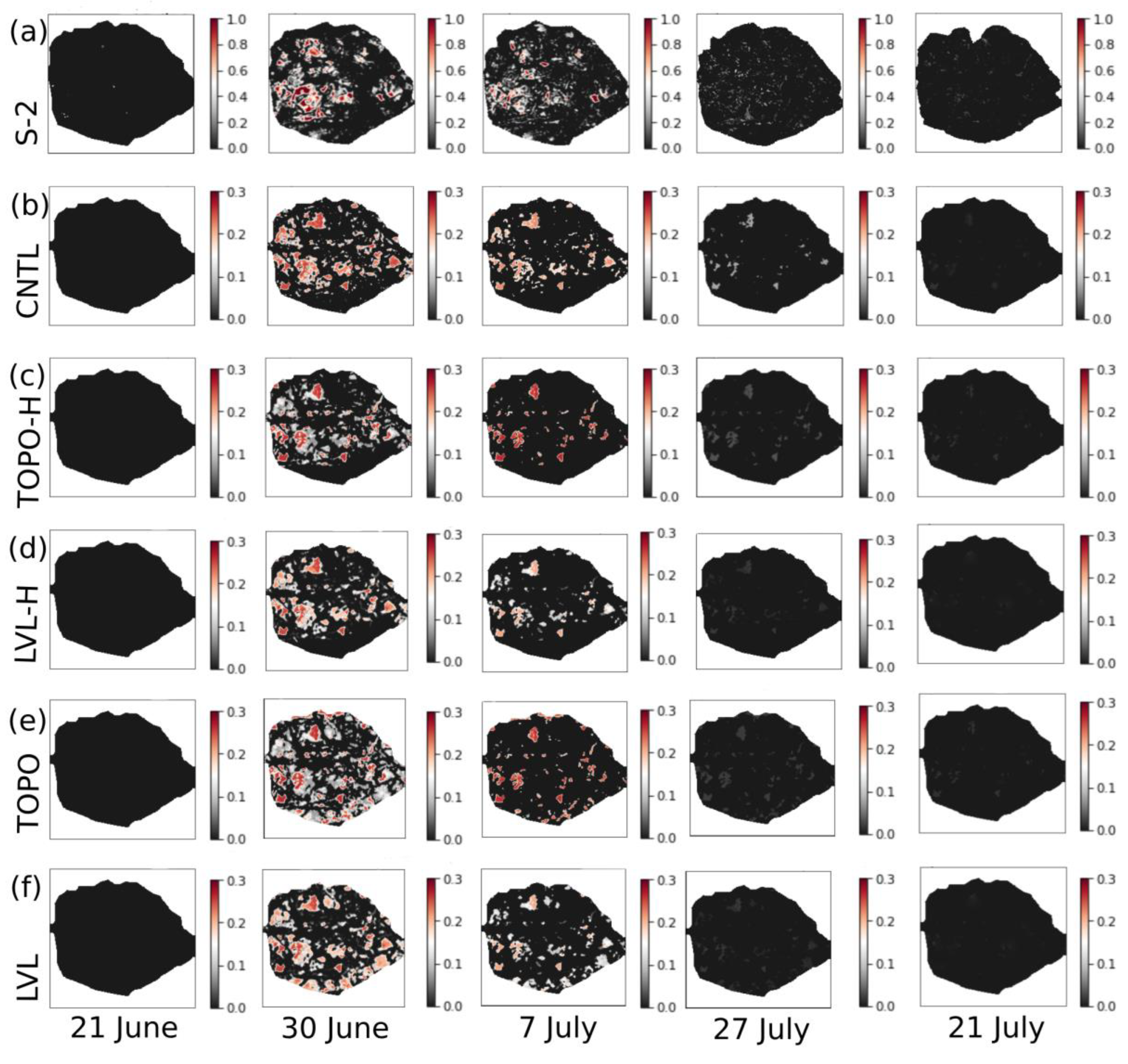
To further compare the differences between the TOPO-H, LVL-H, TOPO, and LVL runs, we investigated the spatial distribution of melt ponds on an example floe at different stages. Figure 6a–f present the simulation results of CNTL, TOPO-H, LVL-H, TOPO, and LVL, respectively. We found that, compared with TOPO and LVL, the spatial distribution of melt ponds in CNTL, TOPO-H, and LVL-H is more consistent with observation. The TOPO and LVL run simulate more melt ponds at the edge of the sea ice than the observations. This can be explained by the lack of macro-flaw outflows in the TOPO and LVL runs. Meltwater accumulated at the edge of the ice floe tends to flow into the ocean rather than gathering into large melt ponds. The spatial correlation between the melt pond distribution of LVL-H and observations is 32.8% higher compared to TOPO-H. This suggests that the melt pond distribution in LVL-H aligns more closely with observations, exhibiting a more uniform distribution across level ice regions. In contrast, the TOPO-H scheme tends to concentrate on melt ponds in areas of lower elevation.
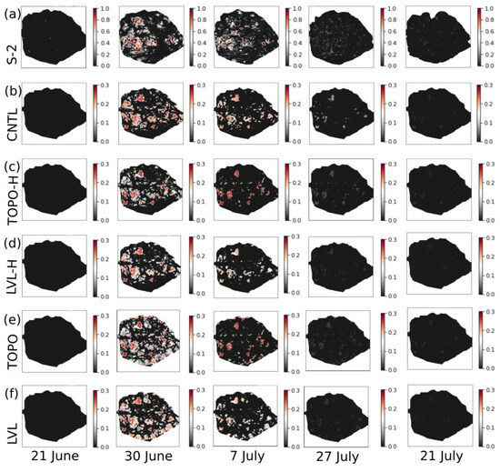
Figure 6.
Comparison of observed and simulated MPF evolution. The dates in each column from left to right are 21 June, 30 June, 7 July, 27 July, and 21 July, respectively. (a) Melt ponds observed from Sentinel-2. (b) Simulated melt pond depth (m) of the CNTL run. (c) Simulated melt pond depth (m) of the TOPO-H run. (d) Simulated melt pond depth (m) of the LVL-H run. (e) Simulated melt pond depth (m) of the TOPO run. (f) Simulated melt pond depth (m) of the LVL run.
Figure 7 illustrates statistical analyses on the simulated melt pond depth of the three schemes. Similar to the spatial distribution of melt ponds, the depth distribution of the CNTL and LVL-H runs is more consistent, exhibiting differences compared to TOPO-H. On 30 June, when the melt pond coverage is at its maximum, the probability density of melt pond depths in CNTL and LVL-H shows a single-peaked distribution, with peaks of less than 0.1 m. In contrast, TOPO-H exhibits a bimodal distribution with more ponds of greater depth. On 7 July, the melt pond depth of CNTL and LVL-H was distributed in the shallow and medium ranges, with the maximum depth being less than 0.15 m. The TOPO-H is single-peak-distributed, with deeper melt ponds being concentrated at around 0.20 m. The simulated results are generally consistent with the MOSAiC observations [35], with the melt pond depths ranging between 0 and 20 cm.
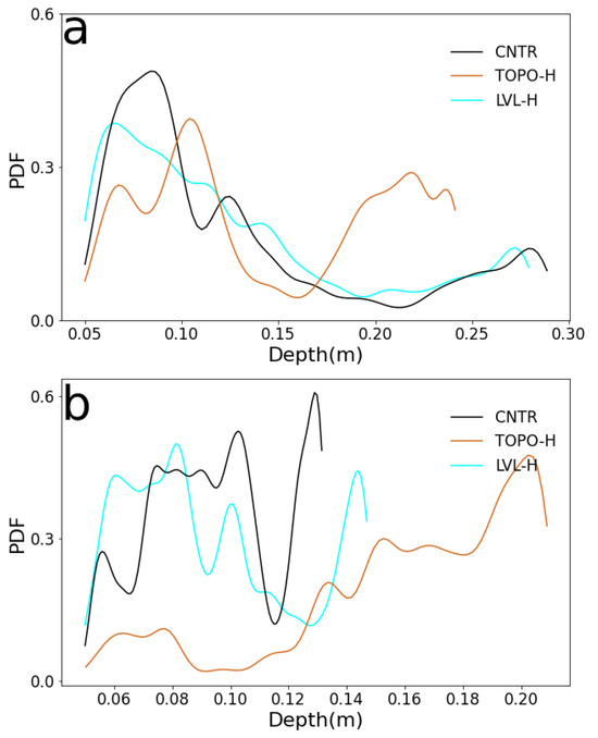
Figure 7.
Simulated probability distribution functions of melt pond depth on (a) 30 June and (b) 7 July.
4.3. Meltwater Budget
To quantitatively investigate the variation in meltwater outflow pathways at different stages and their effects on melt pond evolution, we conducted GRID and RADIAL runs. The GRID run corresponds to a floe with a grid-like distribution of ice ridges and higher ice surface roughness (Figure 8a), whereas the RADIAL run corresponds to a floe with ice ridges extending radially from the center to the edges, exhibiting a radial distribution and 46% lower surface roughness than that of the GRID run (Figure 8b).
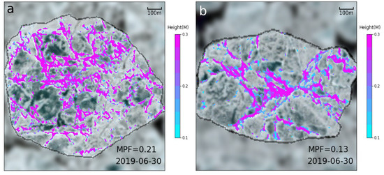
Figure 8.
Initial topography plotted over a true-color Sentinel-2 image of GRID run (a) and RADIAL run (b).
Figure 9 illustrates the variations in total meltwater production and the outflow of meltwater through different pathways during the melting season. The black lines represent the daily amount of generated meltwater, including precipitation. Blue indicates the amount of meltwater outflow to the ocean through vertical drainage and red represents the amount of meltwater flowing to the ocean through macro-flaws. The amount of meltwater generation and loss determines the amount of meltwater stored in melt ponds, thus affecting the surface melt pond coverage of sea ice. The meltwater amount rapidly increases in the early melting stages, then slowly increases and remains stable during the melting season. Before reaching the maximum MPF on 30 June, meltwater generation experiences a rapid increase during this period; additionally, the vertical drainage rate of sea ice is negligible, with the majority of meltwater loss occurring through macro-flaws. This explains the significant improvement in simulation accuracy after adding macro-flaw meltwater outflows in TOPO-H and LVL-H. After reaching the maximum MPF, vertical drainage increases and horizontal macro losses decrease. Therefore, the simulation accuracy of TOPO-H and LVL-H at this stage is not significantly improved compared to TOPO and LVL.

Figure 9.
Meltwater production and drainage of floes with GRID and RADIAL runs over the melting season. The meltwater produced is in the positive numerical range, whereas the meltwater lost has negative numbers.
The influence of ice topography on melt pond evolution has been well established, with studies showing that level sea ice forms a larger melt pond coverage than deformed sea ice during the melting season [36,37,38]. This is mainly based on studies of continuous ice covers. However, this study suggests that exceptions may occur in the case of fragmented ice. In the early stages of the melting season, the RADIAL experiment showed more meltwater draining from the ice edge into the ocean. This was due to the flatter topography and a larger horizontal area connected to the ocean, resulting in a lower maximum melt pond fraction (MPF). In the GRID experiment, a more dispersed network of small melt ponds formed, disconnected from the ice edge, due to the grid-like distribution of ice ridges, which prevented meltwater from flowing into the ocean. As a result, horizontal drainage in the GRID experiment was 12% less than in the RADIAL experiment. Despite the higher surface roughness of the sea ice in the GRID run, its maximum MPF was 38% higher than that in the RADIAL run.
This effect of ice morphology on the coverage area of melt ponds is more significant in the marginal ice zone. Geometrically, this is because the length of the total sea ice edge increases with increasing ice fragmentation. We used the Monte Carlo method to simulate the process of random fragmentation of a unit area of sea ice into smaller fragments and statistically analyzed the change in the total length of edges with an increasing number of fragments, as shown in Figure 10. This indicates a significant increase in the macro-flaws in ice floes as the degree of ice fragmentation increases. In the early stages of melting, when meltwater is generated on ice floes with low vertical permeability, meltwater flows out to the ocean through the sea ice edge, resulting in a low maximum MPF.

Figure 10.
The relationship between the number of sea ice breakups and the total length of the ice floe edge. The Monte Carlo method is used to simulate the random breaking of ice floes into smaller fragments. The solid line is the average value and the shadow is the standard deviation.
A limitation of running such a short simulation is the non-representation of multi-year ice. Since we used observational topography data to describe the deformation of multi-year ice, it is sufficient to set the initial sea ice condition instead of a restart from a spin-up.
5. Conclusions
The sea ice model simulations exhibited inaccuracies in simulating melt ponds, and there were significant differences in the simulation results among different parameterization schemes. The differences in the maximum MPF between simulations using different parameterization schemes exceeded 50%. The topo and lvl parameterizations simplified the control of the ice surface terrain on pond formation and the paths of meltwater loss. The topography scheme assumes that meltwater starts accumulating from the global minima, leading to an excessive concentration of meltwater ponds in low-elevation areas. In contrast, lvl improves by evenly distributing meltwater across all flat ice areas, which is more consistent with observations. However, it lacks the parameterization of meltwater loss pathways through macroscopic defects. We propose a new scheme for improvement, explicitly parameterizing the horizontal transport of meltwater controlled by terrain and gravity and the resulting loss through macroscopic defects using the G-D method.
We conducted simulation experiments to test the accuracy of different parameterization schemes and investigate the reasons for simulation errors. The most informative diagnostic of the simulations is the maximum MPF, as it affects the sea ice mass balance through the albedo-feedback mechanism [39,40]. We found that the CNTL run using the new melt pond scheme exhibited the most consistent maximum MPF with observations, while the TOPO and LVL parameterization schemes overestimated the maximum MPF. We referred to the period before the appearance of the maximum MPF as the early melting period, characterized by minimal vertical permeability of sea ice. We compared the spatial distribution of melt ponds simulated by different runs during this period with observational results and found that the CNTL run was also most consistent with observations. In contrast, errors in the LVL run are mainly caused by the increased MPF at the edges of the sea ice, leading to an overestimation of the MPF. This is due to the lack of parameterization of meltwater loss at the ice edge. Similar errors were observed in the TOPO run, with differences from observations being more pronounced in other areas. The study by Webster et al. on the spatiotemporal evolution of melt ponds during the MOSAiC expedition showed that, compared to the observations, both the Community Earth System Model (CESM2) and the Marginal Ice Zone Modeling and Assimilation System (MIZMAS) overestimated the summer melt pond coverage, which is consistent with the conclusions of this study [12]. We further conducted TOPO-H and LVL-H runs, incorporating macro-flaw outflows into the TOPO and LVL schemes. The results showed significant improvements, with the simulation results of LVL-H being consistent with observations and the results of CNTL. This suggests that LVL is more reasonable than TOPO and that its errors are mainly caused by incomplete parameterization of meltwater outflow processes. The inclusion of the parameterization of macro-flaw outflows enhanced the simulation results of the MPF, particularly in the early stages of melt pond evolution when the coverage expands gradually until reaching its maximum value, with less impact on the subsequent stages of coverage stability and decline. This indicates that meltwater loss through macro-flaws may play a dominant role in the early stages of pond development, with its influence varying at different stages of pond evolution.
Based on the G-D method, we simulated the transport of meltwater on realistic sea ice topography. The simulation results showed the dominant role of macro-flaws in the initial stage of melt pond development, which determines an important parameter of sea ice change, the maximum MPF. In contrast to the high-resolution simulations initialized by realistic topography in this study, the ice-thickness distribution function is used to represent topography in CICE. At their intended resolutions, the lvl and topo schemes offer reasonable approximations of melt pond behavior over larger areas, assuming a relatively simple topography (lvl) or coarse topographic variations (topo). However, a high-resolution-based parameterization would likely capture more nuanced interactions between the ice topography and meltwater flow, leading to more accurate simulations in both pond coverage and drainage behavior. When scaled to lower resolutions, the new parameterization would likely outperform the lvl and topo schemes by offering a more physically grounded representation of melt pond evolution, especially in regions with complex ice topography or significant ice fragmentation. We suggest parameterizing macro-flaw outflows using parameters such as the ice size distribution function and lead fraction. The high-resolution model can be used to study the relationship between these parameters and meltwater outflow. Moreover, compared to the finite element method (FEM) and finite volume method (FVM) traditionally used to simulate fluid dynamics, the G-D method is simpler and easier to introduce into existing sea ice models.
Author Contributions
Conceptualization of the study was conducted by M.W. and N.O. The methodology was developed by M.W. with assistance N.O. and M.W., who also conducted the processing and validation of the data. M.W. prepared the original draft. F.L., V.L. and N.O. reviewed and edited the manuscript. The work was conducted under the supervision of N.O. All authors have read and agreed to the published version of the manuscript.
Funding
This research was funded by the Chinese Government Scholarship (201909370082) in the scope of a stipend “Improving Arctic sea ice albedo parametrization using field and remote sensing data”, the Chinese Natural Science Foundation (42076228) and the funding programme Open Access Publikationsfonds.
Data Availability Statement
The Sentinel-2 satellite imagery is available at the Copernicus Open access Hub of the European Space Agency (ESA) under https://scihub.copernicus.eu/dhus/#/home (accessed on 21 January 2023). The meteorological forcing are available through the Atmospheric Radiation Measurement (ARM) User Facility (http://dx.doi.org/10.5439/1025153, accessed on 21 January 2023). The oceanic forcing data are available on PANGAEA (https://doi.pangaea.de/10.1594/PANGAEA.949433, accessed on 21 January 2023). The SIMBA data are available on PANGAEA (https://doi.org/10.1594/PANGAEA.938244, accessed on 21 January 2023). The melt pond evolution model used in this study are available at Earth Observation and Modelling, Department of Geography, Kiel University.
Acknowledgments
The data used in this work were produced as part of the MOSAiC with the tag MOSAiC20192020 and the ProjectID AWI_122_00. The authors thank all individuals who contributed to the R/V Polarstern expedition during the MOSAiC in 2019–2020. The authors thank the European Space Agency for supplying the Sentinel-2 satellite data. This research was funded by the Chinese Government Scholarship in the scope of the stipend “Improving Arctic sea ice albedo parametrization using field and remote sensing data” and the Chinese Natural Science Foundation (42076228). We acknowledge financial support by Land Schleswig-Holstein within the funding programme Open Access Publikationsfonds.
Conflicts of Interest
The authors declare no conflicts of interest.
References
- Fetterer, F.; Untersteiner, N. Observations of melt ponds on Arctic sea ice. J. Geophys. Res. Oceans 1998, 103, 24821–24835. [Google Scholar] [CrossRef]
- Pedersen, C.A.; Roeckner, E.; Lüthje, M.; Winther, J. A new sea ice albedo scheme including melt ponds for ECHAM5 general circulation model. J. Geophys. Res. Atmos. 2009, 114, D08101. [Google Scholar] [CrossRef]
- Flocco, D.; Feltham, D.L.; Turner, A.K. Incorporation of a physically based melt pond scheme into the sea ice component of a climate model. J. Geophys. Res. Oceans 2010, 115, C08012. [Google Scholar] [CrossRef]
- Holland, M.M.; Bailey, D.A.; Briegleb, B.P.; Light, B.; Hunke, E. Improved Sea Ice Shortwave Radiation Physics in CCSM4: The Impact of Melt Ponds and Aerosols on Arctic Sea Ice. J. Clim. 2012, 25, 1413–1430. [Google Scholar] [CrossRef]
- Perovich, D.K.; Grenfell, T.C.; Richter-Menge, J.A.; Light, B.; Tucker, W.B., III; Eicken, H. Thin and thinner: Sea ice mass balance measurements during SHEBA. J. Geophys. Res. Ocean. 2003, 108, 8050. [Google Scholar] [CrossRef]
- Polashenski, C.; Perovich, D.; Courville, Z. The mechanisms of sea ice melt pond formation and evolution. J. Geophys. Res. Oceans 2012, 117, C01001. [Google Scholar] [CrossRef]
- Landy, J.; Ehn, J.; Shields, M.; Barber, D. Surface and melt pond evolution on landfast first-year sea ice in the Canadian Arctic Archipelago. J. Geophys. Res. Oceans 2014, 119, 3054–3075. [Google Scholar] [CrossRef]
- Webster, M.A.; Rigor, I.G.; Perovich, D.K.; Richter-Menge, J.A.; Polashenski, C.M.; Light, B. Seasonal evolution of melt ponds on Arctic sea ice. J. Geophys. Res. Oceans 2015, 120, 5968–5982. [Google Scholar] [CrossRef]
- Eicken, H.; Krouse, H.R.; Kadko, D.; Perovich, D.K. Tracer studies of pathways and rates of meltwater transport through Arctic summer sea ice. J. Geophys. Res. Oceans 2002, 107, SHE 22-1–SHE 22-20. [Google Scholar] [CrossRef]
- Light, B.; Maykut, G.A.; Grenfell, T.C. Effects of temperature on the microstructure of first-year Arctic sea ice. J. Geophys. Res. Oceans 2003, 108, 3051. [Google Scholar] [CrossRef]
- Maus, S.; Schneebeli, M.; Wiegmann, A. An X-ray micro-tomographic study of the pore space, permeability and percolation threshold of young sea ice. Cryosphere 2021, 15, 4047–4072. [Google Scholar] [CrossRef]
- Webster, M.A.; Holland, M.; Wright, N.C.; Hendricks, S.; Hutter, N.; Itkin, P.; Light, B.; Linhardt, F.; Perovich, D.K.; Raphael, I.A.; et al. Spatiotemporal evolution of melt ponds on Arctic sea ice. Elem. Sci. Anthr. 2022, 10, 000072. [Google Scholar] [CrossRef]
- Oggier, M.; Eicken, H. Seasonal evolution of granular and columnar sea ice pore microstructure and pore network connectivity. J. Glaciol. 2022, 68, 833–848. [Google Scholar] [CrossRef]
- Hunke, E.C.; Hebert, D.A.; Lecomte, O. Level-ice melt ponds in the Los Alamos sea ice model, CICE. Ocean Model. 2013, 71, 26–42. [Google Scholar] [CrossRef]
- Hunke, E.; Allard, R.; Bailey, D.A.; Blain, P.; Craig, A.; Dupont, F.; DuVivier, A.; Grumbine, R.; Hebert, D.; Holland, M.; et al. CICE-Consortium/CICE: CICE, version 6.3.1; Zenodo: Geneva, Switzerland, 2022. [CrossRef]
- Taylor, P.D.; Feltham, D.L. A model of melt pond evolution on sea ice. J. Geophys. Res. Oceans 2004, 109, C12007. [Google Scholar] [CrossRef]
- Lüthje, M.; Feltham, D.L.; Taylor, P.D.; Worster, M.G. Modeling the summertime evolution of sea-ice melt ponds. J. Geophys. Res. Oceans 2006, 111, C02001. [Google Scholar] [CrossRef]
- Skyllingstad, E.D.; Paulson, C.A.; Perovich, D.K. Simulation of melt pond evolution on level ice. J. Geophys. Res. 2009, 114, C12019. [Google Scholar] [CrossRef]
- Popović, P.; Abbot, D. A simple model for the evolution of melt pond coverage on permeable Arctic sea ice. Cryosphere 2017, 11, 1149–1172. [Google Scholar] [CrossRef]
- Nicolaus, M.; Hoppmann, M.; Arndt, S.; Hendricks, S.; Katlein, C.; Nicolaus, A.; Rossmann, L.; Schiller, M.; Schwegmann, S. Snow Depth and Air Temperature Seasonality on Sea Ice Derived From Snow Buoy Measurements. Front. Mar. Sci. 2021, 8, 655446. [Google Scholar] [CrossRef]
- Rabe, B.; Heuzé, C.; Regnery, J.; Aksenov, Y.; Allerholt, J.; Athanase, M.; Bai, Y.; Basque, C.; Bauch, D.; Baumann, T.M.; et al. Overview of the MOSAiC expedition: Physical oceanography. Elem. Sci. Anthr. 2022, 10, 00062. [Google Scholar] [CrossRef]
- Shupe, M.D.; Rex, M.; Blomquist, B.; Persson, P.O.G.; Schmale, J.; Uttal, T.; Althausen, D.; Angot, H.; Archer, S.; Bariteau, L.; et al. Overview of the MOSAiC expedition: Atmosphere. Elem. Sci. Anthr. 2022, 10, 00060. [Google Scholar] [CrossRef]
- Krumpen, T.; von Albedyll, L.; Goessling, H.F.; Hendricks, S.; Juhls, B.; Spreen, G.; Willmes, S.; Belter, H.J.; Dethloff, K.; Haas, C.; et al. MOSAiC drift expedition from October 2019 to July 2020: Sea ice conditions from space and comparison with previous years. Cryosphere 2021, 15, 3897–3920. [Google Scholar] [CrossRef]
- Niehaus, H.; Spreen, G.; Birnbaum, G.; Istomina, L.; Jäkel, E.; Linhardt, F.; Neckel, N.; Fuchs, N.; Nicolaus, M.; Sperzel, T.; et al. Sea Ice Melt Pond Fraction Derived From Sentinel-2 Data: Along the MOSAiC Drift and Arctic-Wide. Geophys. Res. Lett. 2023, 50, e2022gl102102. [Google Scholar] [CrossRef]
- Jackson, K.; Wilkinson, J.; Maksym, T.; Meldrum, D.; Beckers, J.; Haas, C.; Mackenzie, D. A Novel and Low-Cost Sea Ice Mass Balance Buoy. J. Atmos. Ocean. Technol. 2013, 30, 2676–2688. [Google Scholar] [CrossRef]
- Lei, R.; Cheng, B.; Hoppmann, M.; Zuo, G. Snow depth and sea ice thickness derived from the measurements of SIMBA buoys deployed in the Arctic Ocean during the Legs 1a, 1, and 3 of the MOSAiC campaign in 2019–2020. PANGAEA 2021. [Google Scholar] [CrossRef]
- Wang, M.; König, M.; Oppelt, N. Partial Shape Recognition for Sea Ice Motion Retrieval in the Marginal Ice Zone from Sentinel-1 and Sentinel-2. Remote Sens. 2021, 13, 4473. [Google Scholar] [CrossRef]
- Wang, M.; Su, J.; Landy, J.; Leppäranta, M.; Guan, L. A New Algorithm for Sea Ice Melt Pond Fraction Estimation From High-Resolution Optical Satellite Imagery. J. Geophys. Res. Oceans 2020, 125, e2019jc015716. [Google Scholar] [CrossRef]
- Hoppmann, M.; Kuznetsov, I.; Fang, Y.-C.; Rabe, B. Raw seawater temperature, conductivity and salinity obtained at different depths by CTD buoy 2019O5 as part of the MOSAiC distributed network. PANGAEA 2021. [Google Scholar] [CrossRef]
- Wang, M.; Oppelt, N. Estimating Early Summer Snow Depth on Sea Ice Using a Radiative Transfer Model and Optical Satellite Data. Remote Sens. 2023, 15, 5016. [Google Scholar] [CrossRef]
- Hunke, E.; Allard, R.; Bailey, D.A.; Blain, P.; Craig, A.; Dupont, F.; DuVivier, A.; Grumbine, R.; Hebert, D.; Holland, M.; et al. CICE-Consortium/Icepack: Icepack, Version 1.3.1; Zenodo: Geneva, Switzerland, 2022. [CrossRef]
- Feltham, D.L.; Untersteiner, N.; Wettlaufer, J.S.; Worster, M.G. Sea ice is a mushy layer. Geophys. Res. Lett. 2006, 33, L14501. [Google Scholar] [CrossRef]
- Briegleb, B.P.; Light, B. A Delta-Eddington Mutiple Scattering Parameterization for Solar Radiation in the Sea Ice Component of the Community Climate System Model (No. NCAR/TN-472+STR); University Corporation for Atmospheric Research: Boulder, CO, USA, 2007. [Google Scholar] [CrossRef]
- Turner, A.K.; Hunke, E.C. Impacts of a mushy-layer thermodynamic approach in global sea-ice simulations using the CICE sea-ice model. J. Geophys. Res. Oceans 2015, 120, 1253–1275. [Google Scholar] [CrossRef]
- Fuchs, N.; von Albedyll, L.; Birnbaum, G.; Linhardt, F.; Oppelt, N.; Haas, C. Sea ice melt pond bathymetry reconstructed from aerial photographs using photogrammetry: A new method applied to MOSAiC data. Cryosphere 2024, 18, 2991–3015. [Google Scholar] [CrossRef]
- Landy, J.C.; Ehn, J.K.; Barber, D.G. Albedo feedback enhanced by smoother Arctic sea ice. Geophys. Res. Lett. 2015, 42, 10714–10720. [Google Scholar] [CrossRef]
- Nasonova, S.; Scharien, R.K.; Haas, C.; Howell, S.E.L. Linking Regional Winter Sea Ice Thickness and Surface Roughness to Spring Melt Pond Fraction on Landfast Arctic Sea Ice. Remote Sens. 2017, 10, 37. [Google Scholar] [CrossRef]
- Wang, M.; Su, J.; Li Tao Wang, X.; Ji, Q.; Cao, Y.; Lin, L.; Liu, Y. Study on the method of extracting Arctic melt pond and roughness information on sea ice surface based on UAV observation. Chin. J. Polar Res. 2017, 29, 436. [Google Scholar] [CrossRef]
- Eicken, H.; Alexandrov, V.; Gradinger, R.; Ilyin, G.; Ivanov, B.; Luchetta, A.; Martin, T.; Olsson, K.; Reimnitz, E.; Pac, R.; et al. Distribution, structure and hydrography of surface melt puddles. Ber. Polarforsch. 1994, 149, 73–76. Available online: https://epic.awi.de/id/eprint/26327/1/BerPolarforsch1994149.pdf (accessed on 21 January 2023).
- Morassutti, M.P.; LeDrew, E.F. Albedo and depth of melt ponds on sea-ice. Int. J. Climatol. A J. R. Meteorol. Soc. 1996, 16, 817–838. [Google Scholar] [CrossRef]


Disclaimer/Publisher’s Note: The statements, opinions and data contained in all publications are solely those of the individual author(s) and contributor(s) and not of MDPI and/or the editor(s). MDPI and/or the editor(s) disclaim responsibility for any injury to people or property resulting from any ideas, methods, instructions or products referred to in the content. |
© 2024 by the authors. Licensee MDPI, Basel, Switzerland. This article is an open access article distributed under the terms and conditions of the Creative Commons Attribution (CC BY) license (https://creativecommons.org/licenses/by/4.0/).