Article

DLD-SLAM: RGB-D Visual Simultaneous Localisation and Mapping in Indoor Dynamic Environments Based on Deep Learning

1
School of Instrument Science and Engineering, Southeast University, Nanjing 210096, China
2
School of Electrical Engineering and Automation, Changshu Institute of Technology, Changshu 215500, China
*
Author to whom correspondence should be addressed.
Remote Sens. 2024, 16(2), 246; https://doi.org/10.3390/rs16020246
Submission received: 24 October 2023 / Revised: 7 December 2023 / Accepted: 15 December 2023 / Published: 8 January 2024

Abstract

:
This work presents a novel RGB-D dynamic Simultaneous Localisation and Mapping (SLAM) method that improves the precision, stability, and efficiency of localisation while relying on lightweight deep learning in a dynamic environment compared to the traditional static feature-based visual SLAM algorithm. Based on ORB-SLAM3, the GCNv2-tiny network instead of the ORB method, improves the reliability of feature extraction and matching and the accuracy of position estimation; then, the semantic segmentation thread employs the lightweight YOLOv5s object detection algorithm based on the GSConv network combined with a depth image to determine potentially dynamic regions of the image. Finally, to guarantee that the static feature points are used for position estimation, dynamic probability is employed to determine the true dynamic feature points based on the optical flow, semantic labels, and the state in last frame. We have performed experiments on the TUM datasets to verify the feasibility of the algorithm. Compared with the classical dynamic visual SLAM algorithm, the experimental results demonstrate that the absolute trajectory error is greatly reduced in dynamic environments, and that the computing efficiency is improved by 31.54% compared with the real-time dynamic visual SLAM algorithm with close accuracy, demonstrating the superiority of DLD-SLAM in accuracy, stability, and efficiency.

1. Introduction

Visual Simultaneous Localisation and Mapping (VSLAM) is capable of accurately sensing the environment and obtaining the position of the robot. The extensive implementation of VSLAM in autonomous vehicles, perception, and robot technology can be attributed to its cost-effectiveness, improved accuracy, and lack of reliance on specialised sensors [1]. In recent years, there have been notable advancements in VSLAM algorithms. Examples of these advancements include ORB-SLAM2 [2], ORB-SLAM3 [3], VINS-Mono [4], SVO [5], and others. The above open source SLAM algorithms have primarily been designed for static environments. However, in dynamic environments, especially when the texture of moving objects is obvious or occupies a large portion of the image, the accuracy and robustness of the system decrease dramatically. The aforementioned issues have garnered interest towards the integration of VSLAM with deep learning technology. As environments with dynamic objects are frequently present in people’s practical application, it is of great practical significance to further develop VSLAM algorithms with stronger robustness, adaptability, and practicality in dynamic environments.
In recent years, the emergence of deep learning technology has brought new opportunities for the improvement of VSLAM. Compared with the traditional SLAM algorithms based on geometry and feature points, the incorporation of deep learning and VSLAM can augment their capacity to address some difficulties and challenges in SLAM problems [6]. There are various factors that may seriously impact the accuracy and reliability of feature detection. The feature extraction and matching segment at the front end of most SLAM algorithms is unable to extract reliable and consistent features in complex dynamic environments, which can lead to problems such as lost feature tracking and positioning failure. Deep learning methods, such as DeepFeat [7] and LIFT [8], have the ability to acquire highly discriminative feature points from large amounts of data. These networks can extract feature points that contain more geometric and semantic information, thus enhancing the accuracy and robustness of the SLAM system.
Deep learning techniques have demonstrated substantial advancements in the fields of target detection and semantic segmentation, among others. Deep learning techniques have been able to achieve high-precision target detection that can identify and locate multiple targets in complex scenes [9]. Therefore, deep learning techniques can be used to preliminarily segment the position and semantic information of objects in the dynamic environment and identify potential dynamic objects, with different techniques detecting objects with different accuracies. Target detection can generally obtain the detection frame of an object, while semantic segmentation and instance segmentation can be used to mask the region of an object, and instance segmentation can distinguish different individuals of the same category. As the accuracy increases, the deep learning network becomes more complex, which can impact the real-time performance of the system when applied to the SLAM system. Therefore, the operational efficiency of the algorithm can be maintained at the expense of target detection accuracy, and at the same time, the geometric information can be used to accurately identify the region of dynamic objects and improve detection accuracy. It is also feasible to improve the efficiency of the algorithm and reduce the unnecessary computational burden by lightweighting the neural network. After detecting possible dynamic objects using deep learning techniques, dynamic feature points can be identified and rejected by geometric methods such as optical flow and motion consistency estimation.
This paper proposes the DLD-SLAM algorithm to solve the positioning problem in dynamic environments. Based on the below work, our algorithm runs much more efficiently than open source algorithms with the same accuracy. The main work is as follows:
  • On the basis of the ORB-SLAM3 algorithm, the GCNv2 tiny network replaces the conventional ORB method to achieve the extraction and matching of feature points, which improves the efficiency and robustness of the system.
  • The lightweight GSConv [10] module is applied to the YOLOv5s network model, which reduces the count of parameters in the network to improve the computational efficiency of the target detection algorithm. Then, the target detection algorithm combines with the depth information of the RGB-D camera to obtain the mask of potential dynamic targets, which helps identify areas where dynamic feature points are located.
  • A novel method for rejecting dynamic feature points was designed based on the dynamic feature point rejection strategy. We propose the concept of dynamic probability based on LK (Lucas–Kanade) optical flow, semantic labels, and the state in the last frame which is added to the tracking thread. Using this method, the real dynamic feature points are rejected, and the static feature points are retained for position estimation. This method can effectively solve the problem of interference with positioning by dynamic objects.
  • Experiments are carried out for the above design: Firstly, feature point detection and matching are verified to prove the accuracy and robustness of the system; Then, the training accuracy and detection results of the lightweight target detection network are analysed. Finally, the performance of position estimation in the dynamic environment is verified by the TUM dataset, which has been demonstrated to improve the efficiency of our algorithm and the effectiveness of our approach when dealing with dynamic objects.

2. Related Work

2.1. Visual SLAM Based on Deep Learning

Current research has shown the potential of deep learning in several segments of Simultaneous Localisation and Mapping (SLAM), including front-end feature extraction, loop detection, and mapping. The following is a detailed review of the integration of visual SLAM with deep learning.
Traditional front-end feature extraction methods such as Scale-invariant Feature Transform (SIFT) and Speeded-Up Robust Features (SURF) have been widely used in SLAM systems. However, these methods are not stable enough to meet the application requirements in some complex scenes. In recent years, feature extraction methods based on deep learning have gradually emerged. These methods extract feature points and descriptors from images using convolutional neural network (CNN). MagicPoint [11] is an end-to-end position estimation network based on deep learning, but it is only applicable when partially regular graphics and poor migration capability are acceptable. D2-Net [12] is a robust CNN-based feature extraction method. It is able to extract stable feature points and descriptors in different scenarios by designing a CNN architecture based on local stability and repeatability evaluation. R2D2 [13] is proposed based on the D2-Net network. The R2D2 algorithm trains both keypoints and descriptors, using part of the detection network to compute an accuracy score for the feature points. SuperPoint [14] is a lightweight feature extraction method that employs an end-to-end training approach using a convolutional neural network for feature point detection and description. This method has low computational complexity while maintaining high performance. GCNv2 [15] is a proposed algorithm based on the GCN network, which obtains binarised feature points and descriptors through neural networks. Experimental results demonstrate that the above method is more accurate and stable than traditional feature extraction methods.
Traditional mapping methods frequently rely on point clouds, yet these methods are difficult to handle for complex scenes. There has been a growing popularity in the utilisation of deep learning-based methodologies for mapping in recent years. VINet [16] employs convolutional neural networks to extract the features of keyframes in an image sequence. Then, it obtains a global map using a convolutional neural network-based triangulation method.
A number of approaches have also emerged to improve the performance of SLAM algorithms by improving deep learning networks. Zhang, R [17] used ShuffleNetV2 to improve the YOLOv5 network. Meanwhile, to achieve semantic extraction in the environment, the segmentation head of the pyramid scene analysis network is added to the head of the YOLOv5 network, giving the improved YOLOv5 network both target detection and semantic segmentation capabilities. The use of YOLOv5 has also emerged as an approach to the problem of mapping in dynamic scenes [18].
In addition to the above methods, deep learning can be applied to different parts of the SLAM system. These studies demonstrate that the integration of deep learning and VSLAM enhanced system performance and offers a diverse array of practical applications.

2.2. Dynamic Visual SLAM

Dynamic visual SLAM can be mainly classified into geometry-based and deep learning-based approaches.
Among the geometry-based methods, Kim [19] modelled the background in the environment to eliminate the influence of moving targets and constructed a pixel-level background likelihood function based on the difference method between depth images. The image sequence can effectively separate the moving targets from the background region. It can be embedded into the DVO-SLAM system [20] to achieve real-time results. Fan [21] solved the problem of dense distribution and the high number of iterations of the standard RANSAC algorithm when selecting the inner points, as well as the polar constraints, to effectively filter out the dynamic points in the image. PFD-SLAM [22] uses a grid-based motion statistics method to ensure accurate matching with RANSAC. It computes homography transformations to extract dynamic regions and uses particle filtering to accurately determine dynamic regions.
Among the deep learning-based approaches, DS-SLAM [23] is based on the ORB-SLAM2 algorithm. SegNet [24], a semantic segment network, combines with optical flow to construct semantic octree graph maps, which reduces the impact of dynamic objects. Detect-SLAM [25] uses SSD networks [26] to achieve semantic segmentation on keyframes and uses SSD networks on a GPU to solve the time efficiency problem. RDS-SLAM [27] adds a semantic thread to ORB-SLAM3, which also performs semantic segmentation on keyframes and updates the motion probability of feature points based on the segmentation results. DynaSLAM [28] is a visual SLAM system with dynamic object recognition and repair that uses Mask-RCNN [29] to detect and eliminate a priori dynamic objects and combines multi-view geometric constraints to locate undetected dynamic objects. However, the system cannot operate in real time due to the operational efficiency of this instance segmentation network. DP-SLAM [30] solves the problem of the inaccurate detection of dynamic points appearing at the boundary edges of the segmentation by determining the probability of moving points based on the previous frames and Bayes’ law. YOLO-SLAM [31] extends ORB-SLAM2 with semantic segmentation and dynamic feature selection threads. The segmentation thread uses YOLOv3 to select known dynamic objects. The dynamic feature selection thread uses geometric-depth RANSAC to distinguish between dynamic and static feature points.
Compared with geometry-based dynamic visual SLAM systems, deep learning-based systems have higher accuracy and stability and can be applied to more complex environments. However, due to the deep learning network, it tends to reduce the efficiency of the system. Therefore, there is still ample opportunity for further research in the field of deep learning-based SLAM. To compensate for these shortcomings, deep learning combined with geometrically constrained SLAM methods has emerged [32,33]. To solve these problems, we propose a dynamic SLAM system, DLD-SLAM, based on feature point extraction by GCNv2-tiny, lightweight YOLOv5s, and a dynamic feature point rejection strategy.

3. Methods

DLD-SLAM is improved based on ORB-SLAM3 for RGB-D cameras, as shown in the flow chart in Figure 1. In addition to the original three threads of tracking, local mapping, and loop closing, a semantic segmentation thread is designed to identify dynamic regions.
As depicted in Figure 1, the RGB images and depth images are obtained from the RGB-D camera. The RGB images are simultaneously passed into the semantic segmentation thread for target detection and the tracking thread for feature extraction, while the depth images are only passed into the semantic segmentation thread to achieve the mask of dynamic objects in combination with target detection. In the semantic segmentation thread, target detection is performed using the GS-YOLOv5s algorithm. It preliminarily determines the potential dynamic elements by obtaining the semantic information and combining the depth images to obtain the mask of the dynamic elements. Different from traditional semantic segmentation, it refers to the depth information and can achieve the same effect as the semantic segmentation mask without using complex neural networks. GS-YOLOv5s is the target detection method as it performs lightweight processing. It improves the algorithm’s efficiency without affecting its performance.
In the tracking thread, the feature points are extracted and matched using the GCNv2-tiny network. This method can be a good solution to the problem of difficulty with feature point extraction in dynamic environments and the difficulty of matching with large viewpoint changes. Furthermore, the dynamic feature point rejection strategy is designed, and potential dynamic objects are judged to determine whether they are real dynamic elements or not, and the dynamic feature points are rejected. The static feature points are retained for position estimation as well as for back-end optimisation, loop closure, and mapping. Using the strategies described above, we improve the system’s accuracy, robustness, and efficiency.

3.1. Feature Extraction and Matching Based on GCNv2-tiny Network

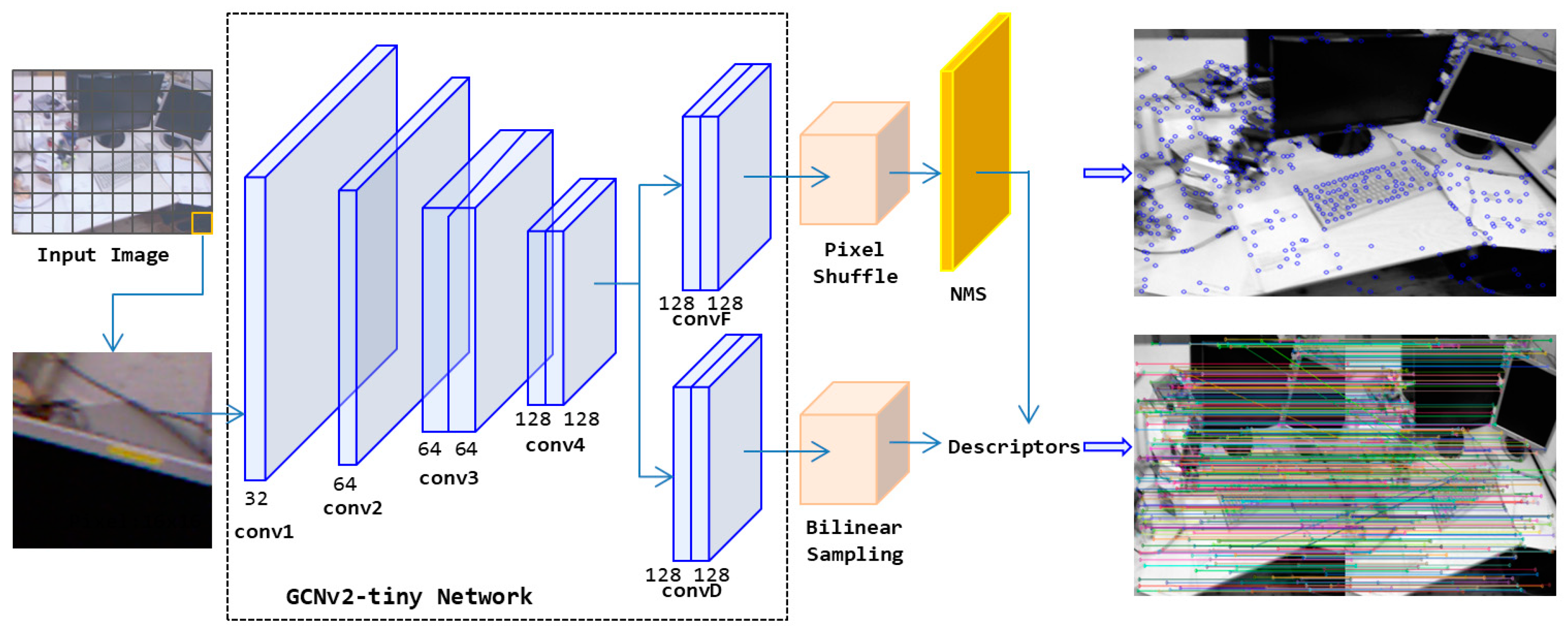
The feature points in the ORB-SLAM3 system are ORB (oriented FAST and rotated BRIEF) feature points. The method of extracting feature points in each frame is as follows: Firstly, an image pyramid of decreasing resolution is constructed by down-sampling. Then, each layer of the image is divided into a 30 × 30 pixel grid, and the feature points are extracted and homogenised in the grid. Finally, the extraction of ORB feature points is repeated for each layer of the image. This method leads to an increase in computation, which reduces the real-time performance of the system. To improve the real-time performance of the system, we employ the GCNv2-tiny network to extract image feature points and descriptors, which replaces the original ORB feature points and is ported to ORB-SLAM3. Figure 2 depicts the process of extracting feature points using the GCNv2-tiny network.
As depicted in Figure 2, firstly, the original input image is segmented into a 16 × 16 pixel grid for separate prediction, which ensures that the feature points are evenly distributed throughout the image. The GCNv2-tiny network shares the convolutional network from conv1 to conv4 to encode image features. Compared to the GCNv2 network, the GCNv2-tiny network halves the number of convolution channels in conv3 and after conv3 while maintaining the same convolution kernel size and step size. This compresses the parameters to reduce the amount of computation, which helps to improve real-time performance. Subsequently, the convF convolutional network is employed for decoding. The sub-pixel convolution is employed to obtain both the position data of the feature points and the probability distribution graph showing the confidence degree. The decoding process employs a convolutional network known as convD. The corresponding descriptors are obtained using the bilinear interpolation method. Finally, the feature points are acquired using the procedure of Non-maximum Suppression (NMS) followed by the identification of corresponding descriptors through indexing.
The GCNv2-tiny network predicts both keypoints and descriptors. The network outputs a probability graph of the keypoint confidence degree and a dense feature graph of descriptors. The probability graph of feature points is binary and the points only take values between 0 and 1. This process becomes a classification problem, which gives better training results. Moreover, this is the same as the feature extraction in ORB-SLAM3, so it can be well ported to ORB-SLAM3. The size of a binary feature vector is set to 256 so that the descriptor has the same bit width as the ORB features and so that the descriptor can be directly embedded into the existing ORB-based visual SLAM. The purpose of the network training aims to match the positions of the points with the value of 1 in the probability graph of the feature points in the final output as closely as possible to the corresponding real feature points in the training dataset. At the same time, a binary activation layer is added at the end of the network to obtain binary descriptors.
By introducing the attention mechanism into the feature encoding stage, more specific feature points can be obtained, which can improve the robustness of feature matching. The GCNv2-tiny network was trained using the SUN3D [34] dataset, which provides information about the camera’s motion position. The network uses sample data as well as a loss function, and it contains not only the true positions of the feature points but also the true feature matching relationships obtained from the real position. And the position information in the dataset is the main training base. Therefore, the feature point matching is more stable when the larger view changes, which is also beneficial to the position estimation based on feature points.
The feature point extraction and matching used in this paper are conducive to improving the real-time performance of the system, and the extracted feature points are more suitable for high-precision position estimation. This algorithm is more stable when dealing with large perspective changes and dynamic object disruptions.

3.2. Lightweight YOLOv5 Target Detection Algorithm

YOLO [35] is a one-stage target detection algorithm that has a simple structure and superior performance in both detection speed and detection accuracy. YOLOv5 can be divided into several different architectures depending on the number of convolutional kernels in the network. YOLOv5 contains five architectures: YOLOv5x, YOLOv5l, YOLOv5m, YOLOv5n, and YOLOv5s. The number of floating point operations and the value of model parameters decrease for these five models in the given order. In this paper, we choose YOLOv5s, which has a smaller number of model floating-point operations and model parametric quantities, because this architecture satisfies the system’s detection accuracy with less computation required as well as a faster rate of model training. Based on the YOLOv5s algorithm, it is lightweighted in this paper.
The YOLOv5s model is mainly composed of Backbone, Neck, and Head, which includes a large number of convolutional neural network (Conv), spatial pyramid pooling fast (SPPF), and CSP [36] modules. The role of Neck is to perform multi-scale feature fusion processing on the feature graph and then to pass the feature graph to the prediction layer, which requires a large number of parameters and computations. In order to reduce the computational effort of the model and build a lightweight network, the convolution network GSConv is added to the CSP2_x module, which is mainly used in the Neck stage. GSConv replaces the standard convolution network with depthwise convolution (DWConv), which reduces the number of parameters and computation by about half compared to the standard convolution. The network improves the efficiency of training and running the model while maintaining a comparable level of performance.
The original input image should be transformed into a multi-layer feature map in Backbone and subjected to feature extraction. Different layers of features are fused together in the Neck module using up-sampling and down-sampling operations. This produces feature graphs with multi-scale information. During these operations, each spatial compression and channel expansion of the feature graph results in the loss of some detection information. Dense convolutional maximises the retention of hidden connections between each channel. Then, a smaller channel is placed in the centre of the GSConv model. This reduces the amount of additive computation while ensuring that effective detection information is delivered. However, due to the deeper layers of the GSConv network model, the deeper network increases the resistance of the data flow. It is therefore not suitable for use in all stages of YOLOv5s.
In Neck, the processed feature graphs are maximised in the channel dimension and minimised in the width and height dimensions. This is a better fit to the structure of the GSConv model as it does not require any transformation to be performed. There is an improvement in performance without a reduction in the efficiency of network inference due to the deepening of the layers. Therefore, a better choice is to use GSConv only at the Neck stage. As shown in Figure 3, the GSConv network is used in the CSP2_x module in the YOLOv5s network, and the GSbottleneck module is added based on GSConv. Based on this, the Neck module is reconstructed, keeping the original structure of the Backbone and Head modules unchanged. In Neck, the multi-scale fusion feature graphs processed by GSConv are less redundant and do not need to be compressed. In addition, the attention module is more effective.

3.3. Dynamic Object Detection Based on Target Detection and Depth Image

The target detection algorithm used in this work is GS-YOLOv5s. This algorithm can only initially determine the potential dynamic objects by semantic labels and represent the dynamic objects with a rectangular detection box. However, if the coverage area of the detection box is large while the proportion of the area occupied by the dynamic objects in that detection box is small, it will result in the rejection of too many static points in the background. This will lead to insufficient static feature points for position estimation and affect the positioning accuracy of the system. Therefore, we adopt the method of combining target detection and depth information to further accurately determine the area of dynamic elements in the image. This is similar to obtaining a mask by semantic segmentation and maximises the retention of static feature points.
Most dynamic objects have some depth difference from the background. In addition, dynamic objects tend to occupy the centre of the detection frame. The four corners of the detection frame basically correspond to the static background points. Figure 4 demonstrates the positional relationships of dynamic objects in space and the meaning of every element.
d max = max d t l ,     d t r ,     d b l , d b r ,
where d t l , d t r , d b l ,   and   d b r  represent the depth values corresponding to the four corner points of this detection frame. The depth of a pixel is assumed to be represented by d. The maximum background depth of a dynamic object is d max . The reason for not selecting the minimum depth is to avoid feature points near or in front of the dynamic element causing the dynamic mask detection to fail.
d - = d c + ϵ , d max d c > ϵ ,
where d c represents the depth value corresponding to the centre of the detection frame. The values of d c     and     d max is used to determine the threshold d - that distinguishes the foreground dynamic feature points from the background static feature points. d - represents the mask depth threshold. The value of ϵ is a pre-determined distance based on empirical values of the frequently occurring positions of dynamic objects in the scene.
The process of obtaining the mask of dynamic objects is as follows: Firstly, we set the depth value of a depth image, but not the target detection frame, to 0. We then set a mask region with the size of the detection frame area where the depth value is d - . And the threshold value ϵ is to ensure that the depth position of the mask region is between the dynamic object and the background. Then, the pixel depth value in the detection box is compared to d - . If it is less than d - , the feature is considered to be in a dynamic region. Otherwise, it is considered a static region, and the depth value is set to 0. The result is a mask that serves the same purpose as semantic segmentation for a more accurate rejection of dynamic feature points.
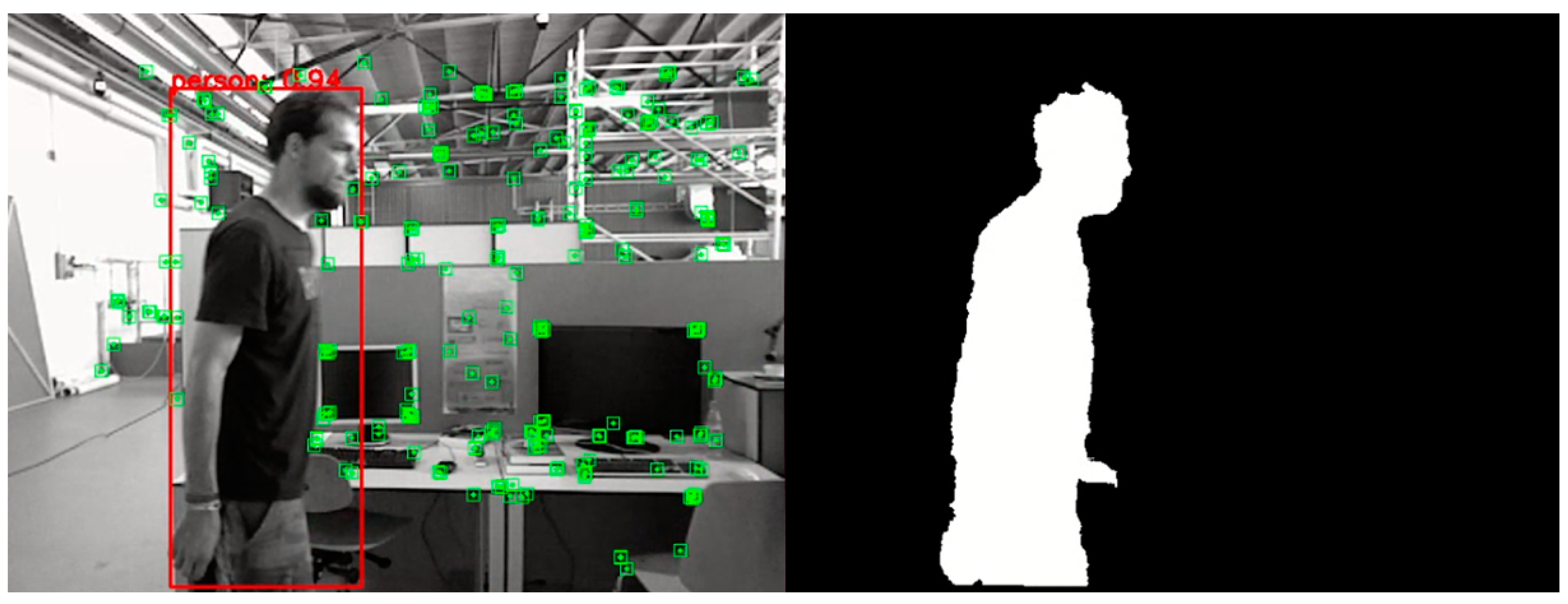
As shown in Figure 5, combining the target detection results with the depth information from the RGB-D camera can obtain results comparable to that of semantic segmentation. Due to the complexity of the semantic segmentation neural network, it will be more computationally intensive, leading to an increase in running time. This may affect the real-time performance of the system. However, our method solves the above problems while ensuring the accuracy of the system.
The method is used to obtain a semantic segmentation mask with the contour of the target object and to avoid culling dynamic feature points by over-culling static feature points in the detection box. Although there are open source semantic segmentation algorithms with this capability, they often do not run in real time. Our approach, by combining a target detection algorithm with depth information, makes full use of the sensor information and also improves the running efficiency of the algorithm.
In a word, the depth information is used to determine the depth in space of all objects in the detection box. The depth of the dynamic objects, d c , and the depth of the static background, d max , are determined. The position of the mask is determined between the depth values d c and d max . It can obtain the mask of the object, which separates dynamic objects in the foreground from static backgrounds by setting the value of ϵ in the detection box.

3.4. Dynamic Feature Point Rejection Strategy Based on Optical Flow

Target detection using the GS-YOLOv5s algorithm is combined with RGB-D depth images to obtain candidate masks of dynamic objects, which are sorted by semantic labels. The real static, potential, or real dynamic objects are then further sorted by dynamic probability based on the optical flow and semantic information, and then the feature points within the dynamic object mask are removed. In real environments, there are different kinds of objects; some objects have the ability to move autonomously, such as people, animals, etc., and they are usually in a state of motion, which is called dynamic objects, while objects such as tables, sofas, etc., usually do not move and are therefore called static objects. The potential dynamic objects are mainly objects that have a greater probability of being moved, such as books and chairs. This method will reduce the false rejection rate and improve the accuracy of the system in dynamic environments.
The optical flow can compare the motion of pixel points in adjacent frames. When processing the dynamic objects in a keyframe, the pixel points on the same dynamic object have the same motion trajectory. Therefore, the motion information of the whole dynamic object can be obtained by judging the motion of one pixel point in the dynamic object. In our method, the LK (Lucas–Kanade) optical flow method [37] is used. The LK optical flow method is a method based on the local lightness change of the image. The LK optical flow belongs to the sparse optical flow, which can ensure the performance effect while the computational amount is small.
In real scenes, the motion state of objects often changes. To address these problems, we design the dynamic probability and update the probability with subsequent data, which can more accurately distinguish between dynamic and static regions. In order to make the recognition of dynamic features robust, the dynamic probability is based on the semantic information, the relative velocity constraints are based on the optical flow, and there are three ways to update the feature point state in the last frame. The dynamic probability of the feature point update formula is as follows:
P j X i = α 1 S j X i + α 2 M j X i + α 3 K j 1 X i
where X i represents a feature point on the j-th frame. P j X i represents the probability that the feature point X i in the current frame is a dynamic feature point. S j X i represents the feature points classified by the semantic information which are located in the static, potential dynamic, and dynamic object masks. M j X i represents the result of the verification using the optical flow method. The result that satisfies the threshold takes the value of 1; otherwise, it is 0. K j 1 X i represents the result of the verification of the feature point that matches the feature point X i in the last frame and takes the value of 1 if it has been judged to be a dynamic feature point in the last frame; Otherwise, it takes the value of 0. The value is also set to 0 if the matching feature point is not searched. The values of α are weighting factors and satisfy the constraint that α 1 + α 2 +   α 3 = 1 where the values of α 1 ,   α 2 , α 3 can be adjusted according to the specific environment.
The feature points within the mask are identified by the dynamic feature points waiting to be determined. It is assumed that the set P contains all feature points in the mask. Set D is the set of dynamic feature points, and it set the value of S j X i to 1; set H is the set of feature points within the potential dynamic object mask, and it sets the value of S j X i to 0.5; and set S is the set of static feature points, and it sets the value of S j X i to 1. Furthermore, set P can be expressed as P = DHS.
The results of M j X i  are based on the optical flow method. Each feature point has coordinate and velocity information, which are calculated using the feature extraction algorithm and the optical flow method. In a real scene, the motion of dynamic objects will generate optical flow, and the background will also generate optical flow with the motion of the camera. Therefore, the average motion velocity of all static feature points in the set S needs to be calculated first for the accurate rejection of dynamic feature points. The motion velocity of static feature points is calculated as follows:
U V = 1 N k = 1 n   u k v k ,
where U and V are the average motion velocity of the static feature point along the X- and Y-axis.
The motion velocity of the static feature points is used to identify all feature points in the potential dynamic object masks within set P. The equation for determining the results of M j X i can be expressed as
u k U 2 + v k V 2 > t ,   k = 1 , 2 , n ,
where t is a self-adaptive threshold.
If the motion velocity of the feature point is beyond this threshold, the value of M j X i is considered to be 1, otherwise the value is 0.
Finally, we determine whether a feature point located in a mask is truly dynamic by the probability P j X i . The feature point which is determined to be a dynamic feature point will be rejected and will not be involved in the position estimation. The method used to reject dynamic feature points is shown in Algorithm 1.
Algorithm 1: Dynamic feature points rejection algorithm.
Input: Current frame’s feature points X i in the semantic segmentation mask, X i P ;
Output: The set S r e a l including all current frame’s static feature point;
1 Obtain all feature points in the semantic segmentation mask belong to the set P;
2 Classify feature points in the set P according to the mask’s semantic labels, X i d m D , X i h m H , and X i s m S , and assign semantic labels to every feature point, S j X i d m =1, S j X i h m =0.5, and S j X i s m =0;
3 for each feature point p i P  do
4 Calculate the mean motion velocity U V = 1 N k = 1 n   u k v k  of all the feature points, X i s j , and calculate the velocity, V p i =   u i U 2 + v i V 2 ;
5  if  V p i > t  then
6    M j p i =1;
7  else  M j p i =0;
8  end if
9 Follow the method in step 5~8, judge the state of p i in last frame, and obtain the value of K j 1 p i ;
10 Calculate the dynamic probability of p i , P j p i = α 1 S j p i + α 2 M j p i + α 3 K j 1 p i ;
11  if  P j p i < ε  then
12   Save the feature points  p i  to the set  S r e a l ;
13  else reject the feature point p i ;
14  end if
15 end for
In step 2, X i d m represents the i-th feature point in the m-th dynamic detection box, X i h m represents the i-th feature point in the m-th potential dynamic detection box, and X i s m represents the i-th feature point in the m-th static detection box.

4. Experimental Results

This section presents experimental details to validate the proposed DLD-SLAM system. In order to evaluate and analyse the proposed DLD-SLAM system, the experiments are performed on a laptop with the following specifications: Intel Core i9-13800H processor, 16 GB RAM, NVIDIA GEFORCE GTX-4600, and 8 GB graphics memory which installed on Lenovo ThinkBook 16 computer. And the operation system is Ubuntu 20.04. The proposed DLD-SLAM algorithm is compared and studied in regards to three aspects: feature extraction and matching, target detection algorithm, and the positioning accuracy of the system. Through the experimental comparison, we demonstrate the superiority of the proposed method.

4.1. Feature Extraction and Matching

In order to verify the feature point extraction and matching effect of the GCNv2-tiny network, we selected the v_bird sequences in the HPatches dataset for the experiments comparing the matching effect of the GCNv2-tiny feature points and ORB feature points. The HPatches dataset is mostly used in the evaluation of image matching and description tasks of transformations of scale, view angle, luminance, etc. And each sequence has the exact corresponding feature points and the truth of the transform parameters. It can be used for the validation of the effectiveness of feature point extraction and matching methods.
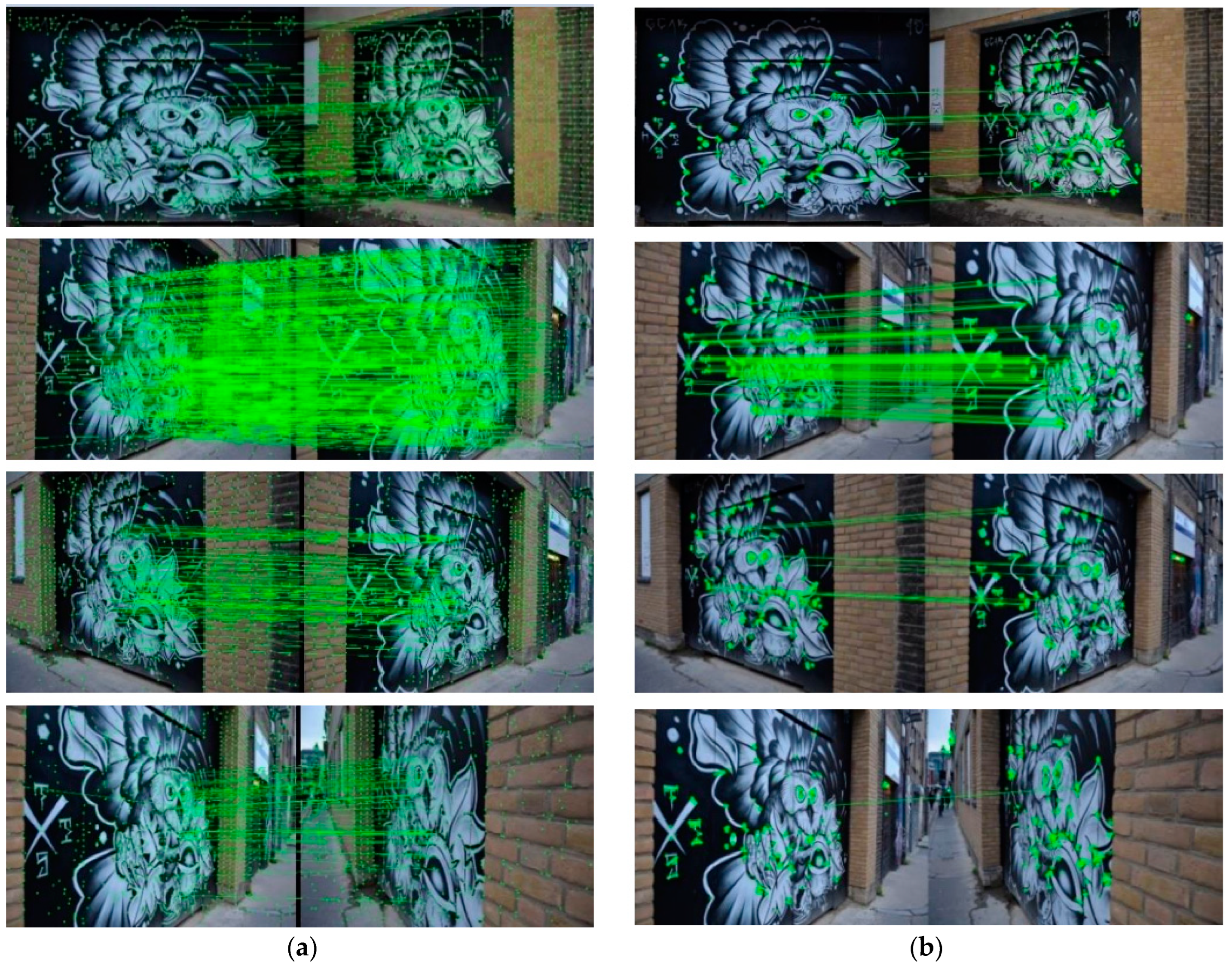
The v_bird sequence within the HPatches dataset has some images from different viewpoints of the same scene. Figure 6 illustrates the impact of GCNv2-tiny and ORB feature extraction and matching across various viewing angles. When the viewing angle is not changed much, ORB has a good matching effect, but when the viewing angle is changed a lot, ORB has almost no matching effect. The GCNv2-tiny model demonstrates a robust capacity for matching. Regardless of variations in the viewing angle, the feature points can be matched. The results are presented in Table 1.
In Table 1, correct matches refer to the initial matches after the RANSAC algorithm has removed the false matches. The rate represents the proportion of correct matches to the number of initial matches. For small changes in perspective, the GCNv2-tiny feature point shows a significantly higher correct match rate over ORB. It can be concluded that the GCNv2-tiny feature points are more adaptable and robust in complex scenes with large perspective changes.

4.2. Target Detection Network Training and Performance

To verify the performance of the GS-YOLOv5s dynamic target recognition algorithm in this paper, the COCO dataset is used for training and validation. The training model for GS-YOLOv5s is performed first. The parameters of the experiment are set as follows: the network training batch size is 128, the initial learning rate is 0.01, the weight decay coefficient is 0.0005, and the total number of training rounds is 200. During the training process, the dataset is divided into three parts: the training set, the validation set, and the test set. The role of the training set is to train the model to obtain the parameters to make the model fit the data, the role of the validation set is to evaluate the performance of the model and select the best hyperparameters to avoid overfitting the model; and the role of the test set is to test the model’s ability to generalise and to evaluate its performance on an unknown dataset. Figure 7 illustrates the progression of loss values throughout the training process. The accuracy of target detection and classification increases as the loss value decreases, approaching the true value.
As seen from Figure 7, as the number of training rounds increases, the loss decreases and tends to stabilise, and the model gradually converges. The target detection effect of the GS-YOLOv5s model in this paper is comparable than that of YOLOv5s. Combined with the loss curves of the validation set, it can be seen that the model does not show any overfitting phenomenon when applied to the validation set. The model is trained to learn effective features and does not rely too much on the training data.
From Figure 8, the fluctuations in precision and recall gradually decrease and become stable as the number of training rounds increases. And the precision of the YOLOv5s model fluctuates more during the training process. This indicates that its training effect is not as good as the GS-YOLOv5s model in this paper. However, it can be seen from its precision curve that its prediction effect is slightly higher than that of the model in this paper. The corresponding mAP performance indices are presented in Table 2 and were used to evaluate the training results.
Table 2 presents a comparison between the two models in terms of performance parameters. The variable mAP is used to measure the prediction accuracy, and a higher the value represents a better performance. FPS is used to measure the running efficiency; a larger value represents a faster rate. Params is used to measure the model size; the smaller the value, the lighter the model. FLOPs is used to measure the speed of the algorithm; a smaller value represents a faster speed. It can be seen that GS-YOLOv5s is slightly inferior to the original algorithm in accuracy, but the running efficiency is significantly improved over the original algorithm. The proposed methodology demonstrates a 20.54% enhancement in speed, while accompanied by a 0.87% decrease in accuracy. Therefore, the algorithm proposed in this paper improves the running speed by reducing the accuracy slightly to enhance the real-time performance of the system.
The experimental results of the comparison are depicted in Figure 9. The majority of objects within the environment can be effectively detected, although the level of accuracy in detection is not as high as that achieved by YOLOv5s. The classification results are also slightly worse than those of the original algorithm. However, the target detection algorithm in this paper is used to further identify the dynamic objects and does not require strict semantic information for classification. The method employed in this study demonstrates a high level of accuracy in target detection, thereby satisfying the system’s requirements.
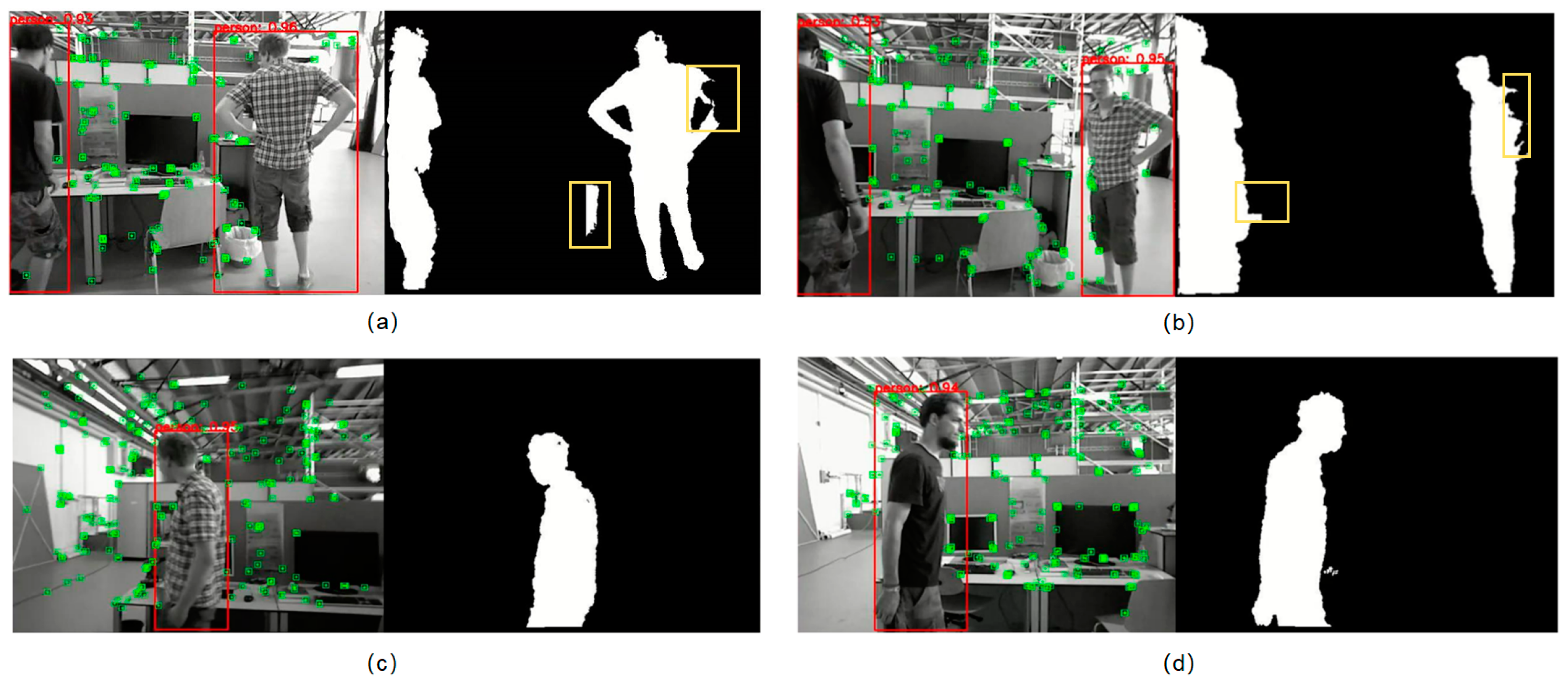
From Figure 10, the mask of dynamic target objects is obtained. In Figure 10a,b, we mark the defects of the detection results by the yellow frame. In Figure 10a, this result is due to the fact that the dynamic object is too close to the neighbouring background, and the depth values of both are close enough to cause the distinction to fail. In Figure 10b, this result is due to the fact that the dynamic object is close to the camera. In the results of all frames, the defects are very rare, and they tend to take up a tiny area of the mask, which will not affect the performance of the system.

4.3. Trajectory Accuracy Verification Experiment in the Dynamic Environment

4.3.1. Trajectory Accuracy

The main metrics used to evaluate trajectories in Visual SLAM are absolute trajectory error (ATE) and Relative Pose Error (RPE). The ATE metric is used to measure the difference between the camera pose estimated by the algorithm and the true camera pose and is used to calculate the global consistency of the trajectory. The ATE metric is used to measure drift in the visual odometer system. And the smaller the ATE evaluation metric, the higher the accuracy. It is assumed that the visual odometry estimate of the position is denoted as P 1 , P 2 , P n S E 3 . S E 3 is the three-dimensional Euclidean transformation consisting of rotations and shifts. The true bit positions of the camera are denoted as Q 1 , Q 2 , Q n S E 3 . These positions represent the camera’s position relative to the world coordinate system at different times or in different frames. The definition of the ATE formulation is given below.
The absolute trajectory error at frame i is defined as
F i = Q i 1 S P i ,
The root mean square error (RMSE) formula for ATE is defined as
R M S E F 1 : n = 1 m i = 1 m   t r a n s F i 2 ,
where the trans . denotes the translational component of the relative trajectory error.
This work focuses on evaluating the trajectory accuracy using ATE.
The TUM_RGBD dataset, an open source dataset provided by the Technical University of Munich in Germany, is used to validate the robustness of the algorithm and the positioning accuracy in dynamic environments. The dataset comprises a total of 39 image sequences depicting various indoor environments. The contents of the dataset encompass both RGB images and depth images. The sitting and walking sequences are dynamic environments. Specifically, the sitting sequence includes two people positioned in front of a table engaging in small-amplitude movements. On the other hand, the walking sequence involves two people performing larger-amplitude movements as they move around a table. Furthermore, these two dynamic subsequences can be associated with four distinct categories of camera motion. There are four different camera movements that can be observed: (1) halfsphere: the camera moves along the hemisphere with a diameter of 1 m; (2) xyz: the camera moves along the x, y, and z axes; (3) rpy: the camera rotates along the roll, pitch, and yaw axes; and (4) static: the camera is stationary.
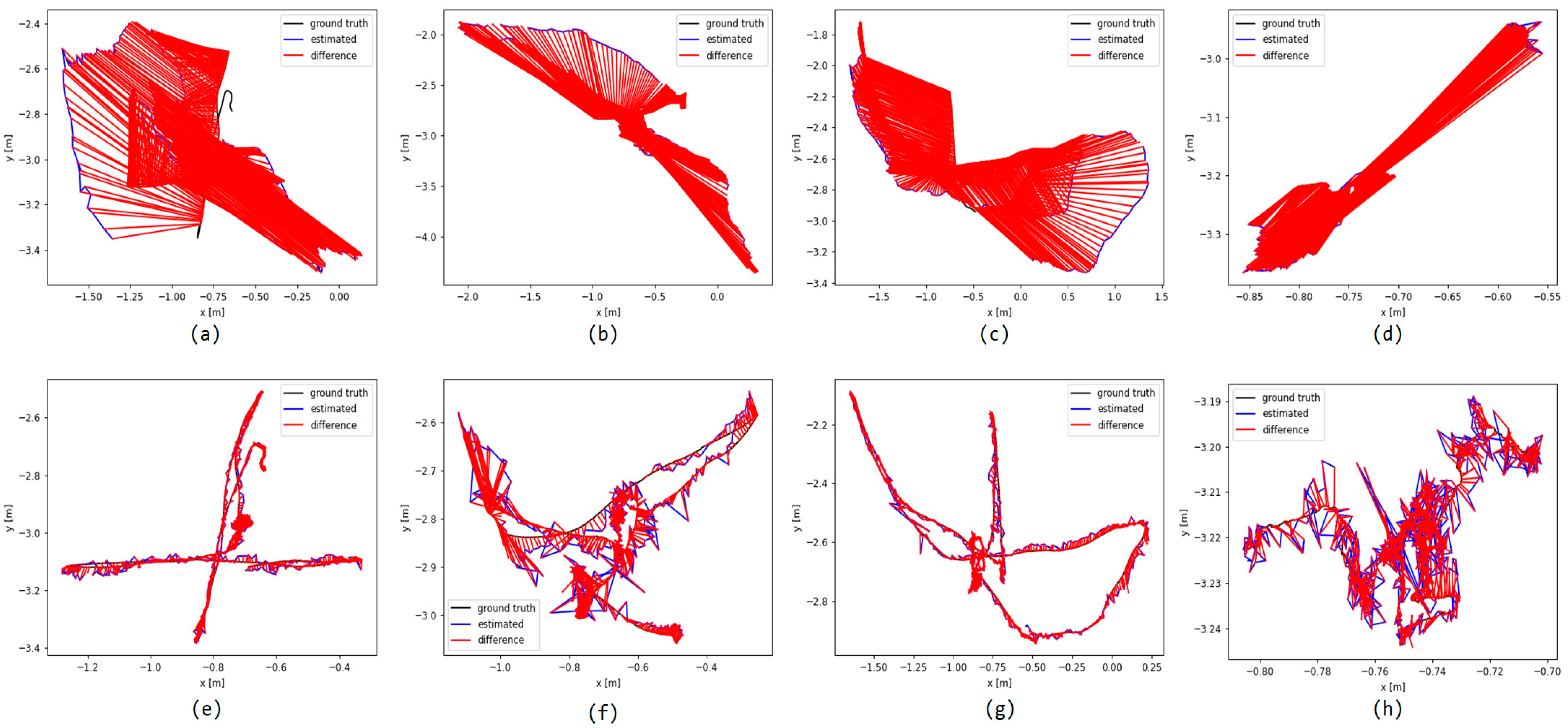
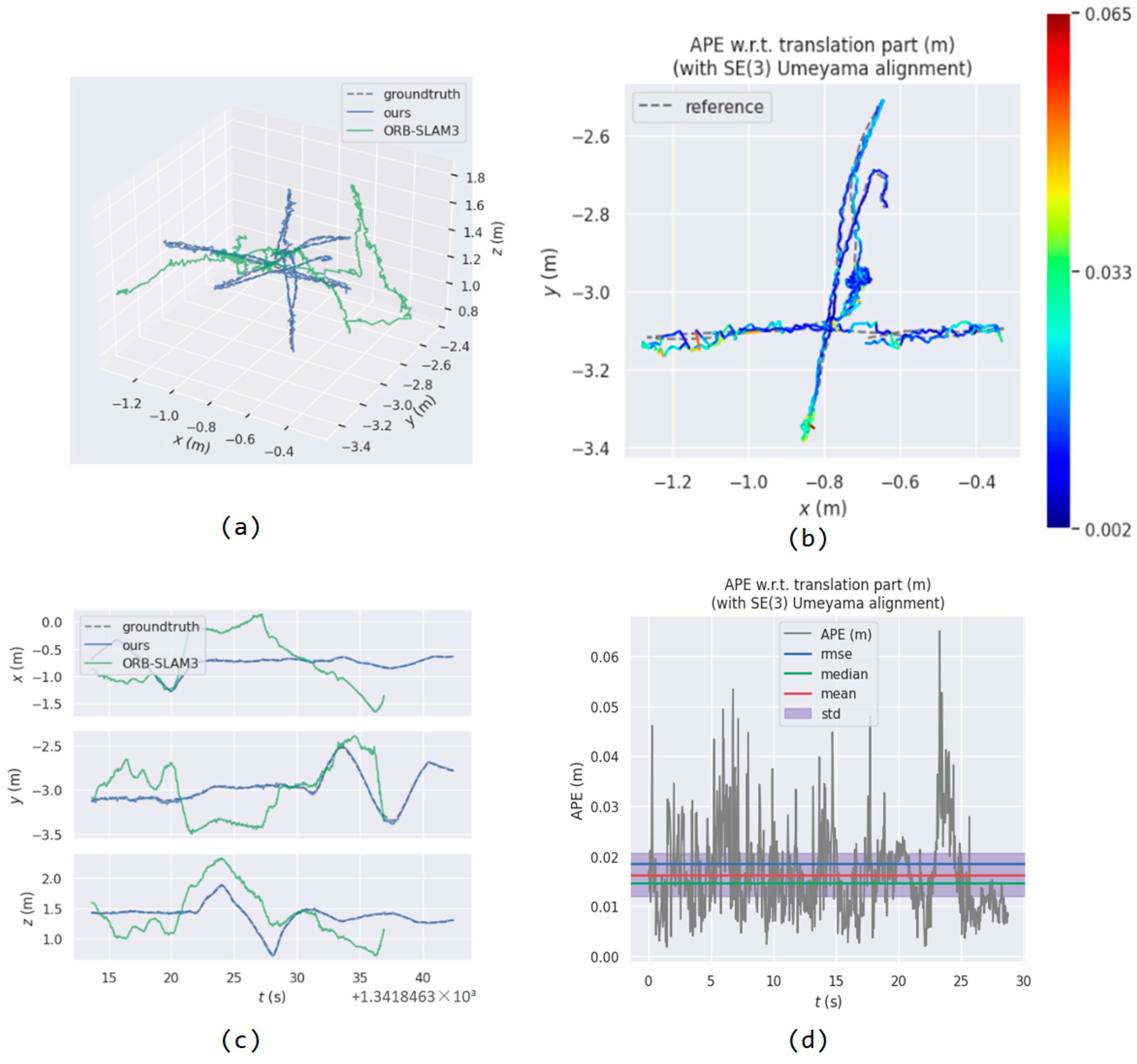
The fr3-walking-xyz, fr3-walking-rpy, fr3-walking-halfsphere, and fr3-walking-static dataset sequences from the highly dynamic environment in the TUM dataset are chosen as the test data. And we compare DLD-SLAM with ORB-SLAM3 to demonstrate the effectiveness of dealing with dynamic interference. Furthermore, the EVO evaluation tool is employed to measure the absolute trajectory error, which quantifies the difference between the estimates provided by the SLAM system and the actual values obtained from the dataset. Figure 10 displays the ATE of the ORB-SLAM3 and DLD-SLAM methods. The red line indicates the distance between the true value and the estimated value, commonly referred to as the absolute trajectory error (ATE). The results of localisation in the TUM dataset are depicted in Figure 11 and Figure 12.
It is evident that DLD-SLAM has a substantial impact on enhancing the precision of localisation in visual SLAM systems operating within dynamic indoor environments.
The experimental findings, as presented in Table 3, indicate that DLD-SLAM demonstrates significantly enhanced accuracy in comparison to ORB-SLAM3; the ATE is greatly reduced. The RMSE is reduced by 97.29%, 94.71%, 96.89%, and 98.61% for the fr3-walking-xyz, fr3-walking-rpy, fr3-walking-halfsphere, and fr3-walking-static sequences. And the robustness of the camera’s various irregular movements performs better when dealing with different sequences.
Table 4 presents the absolute trajectory error RMSE of ORB-SLAM3, DS-SLAM, Detect-SLAM, DynaSLAM, and DLD-SLAM. DS-SLAM and Detect-SLAM are similar to DLD-SLAM in that they all use different networks for the semantic segmentation of the dynamic objects and then determine the real dynamic targets for dynamic feature point rejection. Their positioning accuracy is not much different from this paper’s method, and the ATE of DLD-SLAM can be reduced by about 30% at most. In terms of positioning accuracy, DynaSLAM’s exceeds DLD-SLAM’s. DynaSLAM achieves higher accuracy by leveraging the MASK-RCNN network for dynamic target segmentation and incorporating geometric constraints. Nevertheless, the real-time performance of the MASK-RCNN network is limited by its extended duration.
The method presented in this paper demonstrates enhanced capabilities in addressing localisation challenges in the presence of dynamic interference. The results indicate a notable enhancement in both the accuracy and robustness of the localisation. Moreover, it improves the localisation accuracy of real-time algorithms compared to classical dynamic visual SLAM. Although the localisation accuracy is slightly lower than that of DynaSLAM, DLD-SLAM makes up for the shortcomings of DynaSLAM in operational efficiency.

4.3.2. The Efficiency of the Algorithm

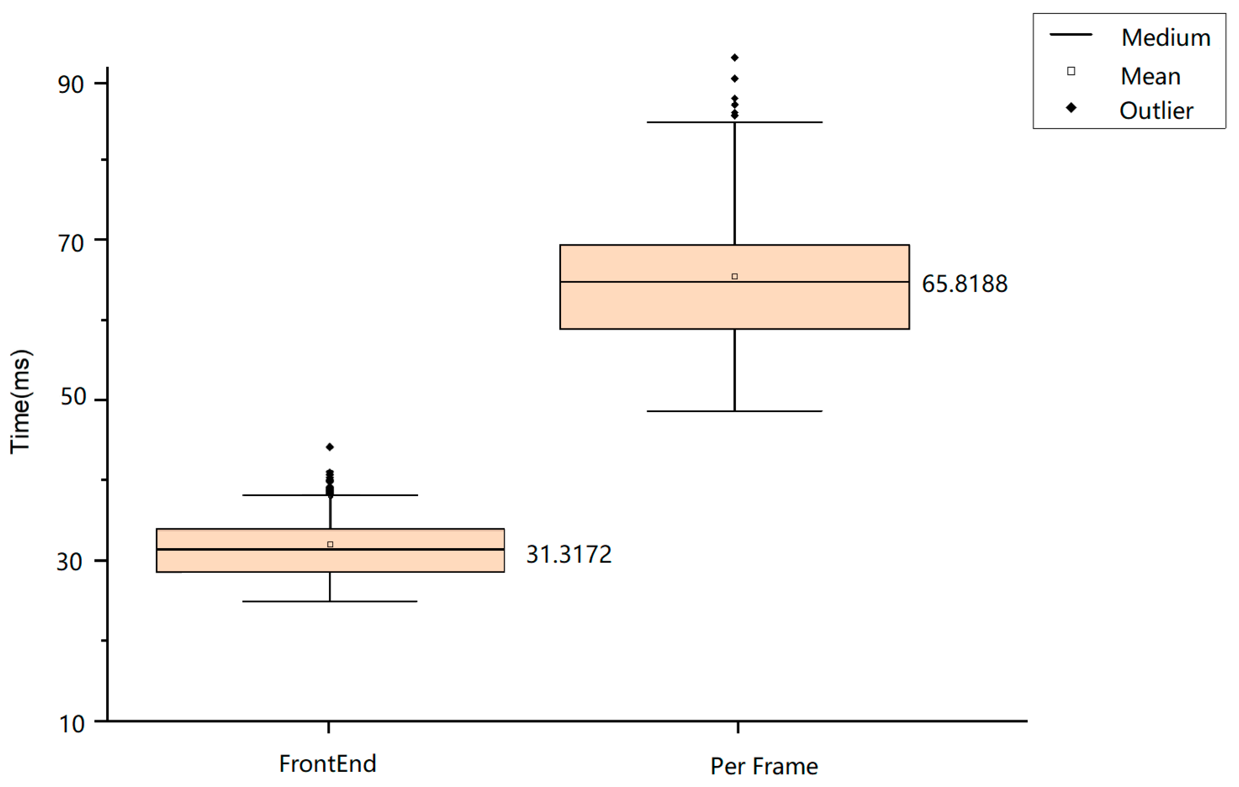
Figure 13 depicts a box plot of the duration taken by this algorithm to process each frame of the fr3_walking_xyz sequence. After removing abnormal values, the time taken to process each frame is between 62 and 68 ms, with a mean value of 65.8188 ms.
Table 5 provides a comparative analysis of the running efficiency of DLD-SLAM and various traditional algorithms in the processing of the fr3-walking-xyz sequence. The time required by each algorithm to process each frame is recorded. One of the considered methods, ORB-SLAM3, does not address the localisation challenge in dynamic environments and includes processes for detecting and rejecting dynamic feature points; consequently, the running time is reduced. DS-SLAM and Detect-SLAM are both examples of dynamic feature point rejection methods, which are employed in the research paper being discussed. However, the method in this paper replaces traditional ORB feature point extraction and matching with a more efficient and stable deep learning method in the front-end session. The integration of a lightweight network and RGB-D depth information is used in dynamic feature point detection and rejection, resulting in enhanced operational efficiency and real-time performance. DynaSLAM cannot run in real-time due to the use of the MASK-RCNN network for segmentation. Therefore, DLD-SLAM demonstrates great superiority in running efficiency in the dynamic visual SLAM algorithm.

5. Discussion

The performance of localisation. The results presented in Figure 6 and Table 1 demonstrate that the DLD-SLAM system successfully extracts a sufficient number of feature points during the feature extraction and matching process. Furthermore, these feature points are matched with greater resilience compared to the conventional ORB features. Figure 7 and Figure 8 demonstrate that our improved target detection method, GS-YOLOv5s, can be effectively trained and predicted. The target detection results depicted in Figure 9 demonstrate that they satisfy the algorithm’s requirements and effectively identify the area where dynamic feature points with semantic labels are situated, when combined with the depth image. Figure 11 and Figure 12, and Table 3 embody the accuracy comparison between DLD-SLAM and ORB-SLAM3 in processing the dynamic sequences of the TUM dataset. It can be seen that the method of this paper can effectively solve the localisation problem of the system in a dynamic environment. By integrating target detection and depth image, the approach successfully acquires object mask and semantic information. Additionally, the adoption of a dynamic feature point rejection strategy further enhances the method’s effectiveness. This method has also proved to be feasible. Table 4 presents a comparative analysis of the positioning accuracy achieved by DLD-SLAM and traditional dynamic SLAM methods; DS-SLAM and Detect-SLAM are the same type of dynamic visual SLAM that can be operated in real-time as this paper, and the accuracy of DLD-SLAM is more superior. This paper presents several contributions that enhance the accuracy of feature point extraction and matching methods. Additionally, it introduces a dynamic feature point rejection method and strategy. The accuracy performance of DynaSLAM surpasses that of other systems; however, its network model lacks the capability to operate in real time. Table 4 illustrates the method’s superior performance in terms of localisation.
The time consumption. Table 2 presents the observed decrease in network parameters of GS-YOLOv5s in comparison to YOLOv5s, along with the corresponding enhancement in running speed. This demonstrates the efficacy of our approach in relation to its compact model size and rapid processing capabilities. Figure 13 demonstrates the running time of DLD-SLAM, including the time consumed per front end and the time consumed per frame. Table 5 embodies the running efficiency comparison between DLD-SLAM and other classical algorithms. The running times per frame of DS-SLAM, Detect-SLAM, and DLD-SLAM are similar in removing the front end time. They differ mainly in the front end time consumed per frame. This reflects our contribution to facilitating the processing of the YOLOv5s algorithm and obtaining semantic segmentation masks by combining them with depth images to improve the running efficiency of the algorithm. DynaSLAM requires more time and does not reach an adequate real-time running performance. In comparison, it is proved that the method in this paper effectively improves the real-time operation of the algorithm.

6. Conclusions

In this paper, a deep learning-based RGB-D visual SLAM algorithm is proposed, which can be applied to dynamic environments and has improved running efficiency. The GCNv2-tiny deep learning method is employed in the tracking thread of ORB-SLAM3, replacing the conventional pyramid-based ORB feature point extraction and matching technique. This method can not only extract enough and uniformly distributed feature points but also has better performance in terms of running efficiency as well as robustness. And the semantic segmentation thread for dynamic targets is added to the original three threads. In this thread, the YOLOv5s target detection network is enhanced through the incorporation of GSConv convolution, which improves the CSP2_x module, resulting in a reduction in the parameters of the deep learning network. In order to meet the system detection accuracy at the same time and improve efficiency, the target detection algorithm needs to be more lightweight. The dynamic targets derived from the target detection process are subsequently integrated with the RGB-D depth data in order to acquire the semantic mask. This approach has the ability to minimise the excessive elimination of static feature points within the detection frame so as to avoid insufficient feature points for position estimation. After determining the mask of the potential dynamic target, this paper adopts the LK optical flow method to judge the relative motion of the feature points in the detection frame by comparing it with the velocity threshold. And the dynamic probability is determined by combining the last frame state of the feature point and the semantic labels. The identification of real dynamic objects is based on the potential dynamic targets. Within the mask region, the dynamic feature points are excluded to ensure that only static feature points are considered for position estimation and optimisation.
The verification of the method’s feasibility and performance is conducted on various sequences from the TUM dataset. In this paper, the algorithm is also evaluated against the ORB-SLAM3, DS-SLAM, Detect-SLAM, and DynaSLAM algorithms in terms of both positioning accuracy and running efficiency. The research results demonstrate a substantial decrease in the absolute trajectory error within dynamic environments. The accuracy of the system increases by approximately 95% when compared to ORB-SLAM3. In comparison to real-time dynamic visual SLAM with its high accuracy, there has been a notable increase of 31.54% in terms of running efficiency. The comprehensive performance of our method demonstrates its superiority. The efficacy of DLD-SLAM in enhancing positioning accuracy, operational efficiency, and robustness in dynamic environments has been substantiated.
In the future, improvements will be made in the following aspects: Sensors such as IMU and LIDAR will be implemented. By broadening the scope of application, it is possible to enhance the accuracy and robustness of the system. The enhancement of running efficiency in deep learning networks can be accomplished by implementing lightweighting techniques such as model pruning. Moreover, it is reasonable to improve system performance by using faster and more accurate target detection methods, such as YOLOv7 and so on. Additionally, taking advantage of semantic information can facilitate the construction of a comprehensive semantic map, which can improve the representation of information in a more complete scene.

Author Contributions

Conceptualisation, Q.W.; methodology, H.Y.; software, H.Y.; validation, H.Y.; formal analysis, H.Y.; investigation, H.Y. and L.L.; resources, H.Y.; data curation, H.Y.; writing—original draft preparation, H.Y.; writing—review and editing, C.Y. and Y.S.; visualisation, H.Y.; supervision, C.Y., Y.F., and Q.W.; project administration, Q.W. and C.Y.; funding acquisition, Q.W. All authors have read and agreed to the published version of the manuscript.

Funding

This research was funded by the National Natural Science Foundation of China (No. 42074039). The authors would like to thank the referees or their constructive comments.

Data Availability Statement

Publicly available datasets were analysed in this study. These data can be found here: TUM dataset: https://cvg.cit.tum.de/data/datasets/rgbd-dataset (accessed on 1 August 2023); COCO dataset: https://cocodataset.org/#download (accessed on 1 August 2023); HPatches dataset: https://github.com/hpatches/hpatches-dataset (accessed on 1 August 2023); the EVO evaluation tool: https://github.com/MichaelGrupp/evo (accessed on 1 August 2023).

Conflicts of Interest

The authors declare no conflict of interest.

References

  1. Abaspur Kazerouni, I.; Fitzgerald, L.; Dooly, G.; Toal, D. A Survey of State-of-the-Art on Visual SLAM. Expert Syst. Appl. 2022, 205, 117734. [Google Scholar] [CrossRef]
  2. Mur-Artal, R.; Tardós, J.D. ORB-SLAM2: An open-source slam system for monocular, stereo, and rgb-d cameras. IEEE Trans. Robot. 2017, 33, 1255–1262. [Google Scholar] [CrossRef]
  3. Campos, C.; Elvira, R.; Rodríguez, J.J.G.; Montiel, J.M.M.; Tardos, J.D. ORB-SLAM3: An Accurate Open-Source Library for Visual, Visual–Inertial, and Multimap SLAM. IEEE Trans. Robot. 2021, 37, 1874–1890. [Google Scholar] [CrossRef]
  4. Qin, T.; Li, P.; Shen, S. VINS-Mono: A Robust and Versatile Monocular Visual-Inertial State Estimator. IEEE Trans. Robot. 2018, 34, 1004–1020. [Google Scholar] [CrossRef]
  5. Forster, C.; Pizzoli, M.; Scaramuzza, D. SVO: Fast semi-direct monocular visual odometry. In Proceedings of the 2014 IEEE International Conference on Robotics and Automation (ICRA), Hong Kong, China, 31 May–7 June 2014. [Google Scholar]
  6. Chengqi, D.; Kaitao, Q.; Rong, X. Comparative Study of Deep Learning Based Features in SLAM. In Proceedings of the 2019 4th Asia-Pacific Conference on Intelligent Robot Systems (ACIRS), Nagoya, Japan, 13–15 July 2019; IEEE: Piscataway, NJ, USA, 2019; pp. 250–254. [Google Scholar]
  7. Mohamed, A.; Tharwat, M.; Magdy, M.; Abubakr, T.; Nasr, O.; Youssef, M. DeepFeat: Robust Large-Scale Multi-Features Outdoor Localization in LTE Networks Using Deep Learning. IEEE Access 2022, 10, 3400–3414. [Google Scholar] [CrossRef]
  8. Yi, K.M.; Trulls, E.; Lepetit, V.; Fua, P. LIFT: Learned Invariant Feature Transform. In Proceedings of the Computer Vision—ECCV 2016, Amsterdam, The Netherlands, 11–14 October 2016; Leibe, B., Matas, J., Sebe, N., Welling, M., Eds.; Springer International Publishing: Cham, Switzerland, 2016; pp. 467–483. [Google Scholar]
  9. Ballester, I.; Fontán, A.; Civera, J.; Strobl, K.H.; Triebel, R. DOT: Dynamic Object Tracking for Visual SLAM. In Proceedings of the 2021 IEEE International Conference on Robotics and Automation (ICRA), Xi’an, China, 30 May–5 June 2021; pp. 11705–11711. [Google Scholar]
  10. Li, H.; Li, J.; Wei, H.; Liu, Z.; Zhan, Z.; Ren, Q. Slim-neck by GSConv: A better design paradigm of detector architectures for autonomous vehicles. arXiv 2022, arXiv:2206.02424. [Google Scholar] [CrossRef]
  11. Xie, Y.; Tang, Y.; Tang, G.; Hoff, W. Learning To Find Good Correspondences Of Multiple Objects. In Proceedings of the 2020 25th International Conference on Pattern Recognition (ICPR), Milan, Italy, 10–15 January 2021; pp. 2779–2786. [Google Scholar]
  12. Dusmanu, M.; Rocco, I.; Pajdla, T.; Pollefeys, M.; Sivic, J.; Torii, A.; Sattler, T. D2-Net: A Trainable CNN for Joint Description and Detection of Local Features. In Proceedings of the 2019 IEEE/CVF Conference on Computer Vision and Pattern Recognition (CVPR), Long Beach, CA, USA, 16–20 June 2019; pp. 8084–8093. [Google Scholar]
  13. Revaud, J.; Weinzaepfel, P.; Souza, C.D.; Humenberger, M. R2D2: Repeatable and Reliable Detector and Descriptor. In Proceedings of the 33rd International Conference on Neural Information Processing Systems, Vancouver, BC, Canada, 8–14 December 2019; Curran Associates Inc.: Red Hook, NY, USA, 2019; pp. 12414–12424. [Google Scholar]
  14. DeTone, D.; Malisiewicz, T.; Rabinovich, A. SuperPoint: Self-Supervised Interest Point Detection and Description. In Proceedings of the 2018 IEEE/CVF Conference on Computer Vision and Pattern Recognition Workshops (CVPRW), Salt Lake City, UT, USA, 18–22 June 2018. [Google Scholar] [CrossRef]
  15. Tang, J.; Ericson, L.; Folkesson, J.; Jensfelt, P. GCNv2: Efficient Correspondence Prediction for Real-Time SLAM. IEEE Robot. Autom. Lett. 2019, 4, 3505–3512. [Google Scholar] [CrossRef]
  16. Clark, R.; Wang, S.; Wen, H.; Markham, A.; Trigoni, N. VINet: Visual-Inertial Odometry as a Sequence-to-Sequence Learning Problem. In Proceedings of the AAAI Conference on Artificial Intelligence, San Francisco, CA, USA, 4–9 February 2017; Volume 31. [Google Scholar] [CrossRef]
  17. Zhang, R.; Zhang, X. Geometric Constraint-Based and Improved YOLOv5 Semantic SLAM for Dynamic Scenes. ISPRS Int. J. Geo-Inf. 2023, 12, 211. [Google Scholar] [CrossRef]
  18. Zhang, X.; Zhang, R.; Wang, X. Visual SLAM Mapping Based on YOLOv5 in Dynamic Scenes. Appl. Sci. 2022, 12, 11548. [Google Scholar] [CrossRef]
  19. Kim, D.-H.; Kim, J.-H. Effective Background Model-Based RGB-D Dense Visual Odometry in a Dynamic Environment. IEEE Trans. Robot. 2016, 32, 1565–1573. [Google Scholar] [CrossRef]
  20. Kerl, C.; Sturm, J.; Cremers, D. Dense visual SLAM for RGB-D cameras. In Proceedings of the 2013 IEEE/RSJ International Conference on Intelligent Robots and Systems, Tokyo, Japan, 3–7 November 2013; pp. 2100–2106. [Google Scholar] [CrossRef]
  21. Guohao, F.; Lele, B.; Cheng, Z. Geometric Constraint-Based Visual SLAM Under Dynamic Indoor Environment. Comput. Eng. Appl. 2021, 57, 203–212. [Google Scholar]
  22. Zhang, C.; Zhang, R.; Jin, S.; Yi, X. PFD-SLAM: A New RGB-D SLAM for Dynamic Indoor Environments Based on Non-Prior Semantic Segmentation. Remote Sens. 2022, 14, 2445. [Google Scholar] [CrossRef]
  23. Yu, C.; Liu, Z.; Liu, X.-J.; Xie, F.; Yang, Y.; Wei, Q.; Fei, Q. DS-SLAM: A Semantic Visual SLAM towards Dynamic Environments. In Proceedings of the 2018 IEEE/RSJ International Conference on Intelligent Robots and Systems (IROS), Madrid, Spain, 1–5 October 2018; pp. 1168–1174. [Google Scholar]
  24. Badrinarayanan, V.; Kendall, A.; Cipolla, R. SegNet: A Deep Convolutional Encoder-Decoder Architecture for Image Segmentation. IEEE Trans. Pattern Anal. Mach. Intell. 2017, 39, 2481–2495. [Google Scholar] [CrossRef] [PubMed]
  25. Zhong, F.; Wang, S.; Zhang, Z.; Chen, C.; Wang, Y. Detect-SLAM: Making Object Detection and SLAM Mutually Beneficial. In Proceedings of the 2018 IEEE Winter Conference on Applications of Computer Vision (WACV), Lake Tahoe, NV, USA, 12–15 March 2018; pp. 1001–1010. [Google Scholar] [CrossRef]
  26. Liu, W.; Anguelov, D.; Erhan, D.; Szegedy, C.; Reed, S.; Fu, C.-Y.; Berg, A.C. SSD: Single Shot MultiBox Detector. In Proceedings of the Computer Vision—ECCV 2016, Amsterdam, The Netherlands, 11–14 October 2016; Volume 9905, pp. 21–37. [Google Scholar]
  27. Liu, Y.; Miura, J. RDS-SLAM: Real-Time Dynamic SLAM Using Semantic Segmentation Methods. IEEE Access 2021, 9, 23772–23785. [Google Scholar] [CrossRef]
  28. Li, A.; Wang, J.; Xu, M. DP-SLAM: A visual SLAM with moving probability towards dynamic environments. Inf. Sci. 2020, 556, 128–142. [Google Scholar] [CrossRef]
  29. He, K.; Gkioxari, G.; Dollár, P.; Girshick, R. Mask R-CNN. In Proceedings of the 2017 IEEE International Conference on Computer Vision (ICCV), Venice, Italy, 22–29 October 2017; pp. 2980–2988. [Google Scholar] [CrossRef]
  30. Bescos, B.; Fácil, J.M.; Civera, J.; Neira, J. DynaSLAM: Tracking, Mapping, and Inpainting in Dynamic Scenes. IEEE Robot. Autom. Lett. 2018, 3, 4076–4083. [Google Scholar] [CrossRef]
  31. Wu, W.; Guo, L.; Gao, H.; You, Z.; Liu, Y.; Chen, Z. YOLO-SLAM: A semantic SLAM system towards dynamic environment with geometric constraint. Neural Comput. Appl. 2022, 34, 6011–6026. [Google Scholar] [CrossRef]
  32. Wei, S.; Wang, S.; Li, H.; Liu, G.; Yang, T.; Liu, C. A Semantic Information-Based Optimized vSLAM in Indoor Dynamic Environments. Appl. Sci. 2023, 13, 8790. [Google Scholar] [CrossRef]
  33. Wang, X.; Zhang, X. MCBM-SLAM: An Improved Mask-Region-Convolutional Neural Network-Based Simultaneous Localization and Mapping System for Dynamic Environments. Electronics 2023, 12, 3596. [Google Scholar] [CrossRef]
  34. Xiao, J.; Owens, A.; Torralba, A. SUN3D: A Database of Big Spaces Reconstructed Using SfM and Object Labels. In Proceedings of the 2013 IEEE International Conference on Computer Vision, Sydney, Australia, 1–8 December 2013; pp. 1625–1632. [Google Scholar]
  35. Redmon, J.; Divvala, S.; Girshick, R.; Farhadi, A. You only look once: Unified, real-time object detection. In Proceedings of the 2016 IEEE Conference on Computer Vision and Pattern Recognition (CVPR), Las Vegas, NV, USA, 27–30 June 2016; pp. 779–788. [Google Scholar] [CrossRef]
  36. Wang, C.-Y.; Liao, H.-Y.M.; Wu, Y.-H.; Chen, P.-Y.; Hsieh, J.-W.; Yeh, I.-H. CSPNet: A New Backbone that can Enhance Learning Capability of CNN. In Proceedings of the 2020 IEEE/CVF Conference on Computer Vision and Pattern Recognition Workshops (CVPRW), Seattle, WA, USA, 14–19 June 2020; pp. 1571–1580. [Google Scholar] [CrossRef]
  37. Lucas, B.D.; Kanade, T. An Iterative Image Registration Technique with an Application to Stereo Vision. In Proceedings of the 7th International Joint Conference on Artificial Intelligence—Volume 2, Vancouver, BC, Canada, 24–28 August 1981; Morgan Kaufmann Publishers Inc.: San Francisco, CA, USA, 1981; pp. 674–679. [Google Scholar]
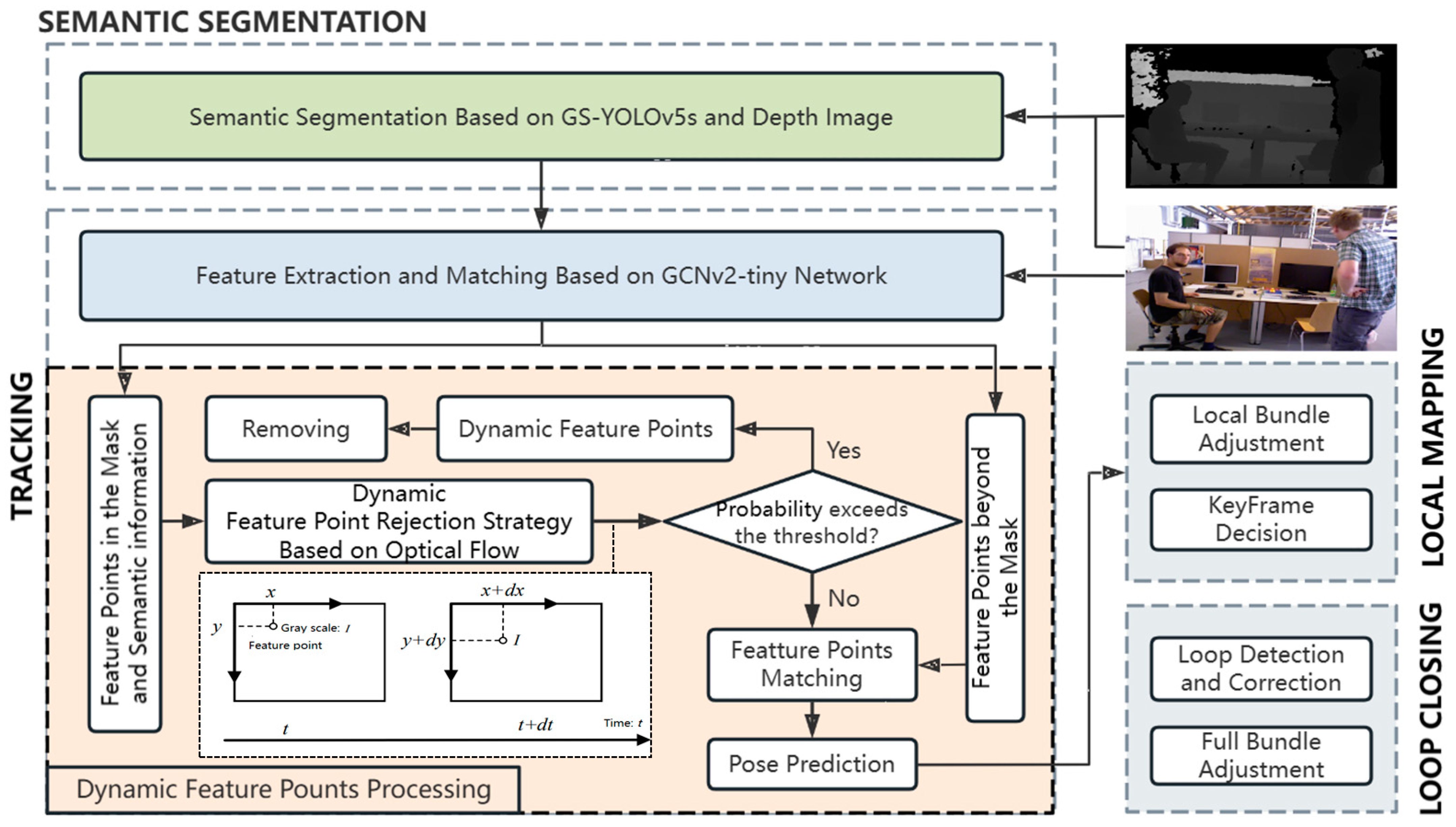
Figure 1. Overview of DLD-SLAM. The algorithmic framework contains four threads: semantic segmentation, tracking, local mapping and loop closing. Section 3.1 is shown in blue; Section 3.2 and Section 3.3 are shown in green; and Section 3.4 is shown in orange to express the process of dynamic feature points rejected.
Remotesensing 16 00246 g001
Figure 2. The procedure of extracting feature points based on GCNv2-tiny network. The number under the convolutional layer in the figure is the number of channels. The two figures on the right show the results of feature point extraction and matching.
Remotesensing 16 00246 g002
Figure 3. The CSP2_x module structure in GS-YOLOv5s network.
Remotesensing 16 00246 g003
Figure 4. This shows the principle of semantic segmentation. (a) Background represents the static objects in the background: A is the static background closer to the corresponding dynamic object in the detection box, and B is the static background further away from the corresponding dynamic element in the detection frame. Different classes of feature points are represented by different colours. (b) Description of distance of various elements in Figure (a) in the camera coordinate system along the z-axis.
Remotesensing 16 00246 g004
Figure 5. The result of semantic segmentation based on our method. The red represents the target detection box; the green represents static feature points in the keyframe. The depth value of white area is 1, while that of the black area is 0.
Remotesensing 16 00246 g005
Figure 6. This figure shows the performance of feature point extraction and matching. From top to bottom, the scenes shows the different perspectives (1~4). (a) The results of the GCNv2-tiny method; (b) the results of the ORB method.
Remotesensing 16 00246 g006
Figure 7. Plot of training loss variation for GS-YOLOv5s model. The variable box_loss is the bounding box regression loss; obj_loss is the confidence loss; cls_loss is the classification probability loss. The variable train represents the loss change in the training set, while val represents the loss change in the validation set.
Remotesensing 16 00246 g007
Figure 8. Plot of changes in performance metrics for GS-YOLOv5s model. The changes in precision, recall, and mAP of GS-YOLOv5s model during the training process. The variable mAP_0.5 refers to a mAP with IoU threshold larger than 0.5; mAP_0.5:0.95 denotes the average mAP at different IoU thresholds (from 0.5 to 0.95, with a step size of 0.05).
Remotesensing 16 00246 g008
Figure 9. The comparison of the detection results of the two algorithms on the test samples. The left and right side show the comparison of target detection results between YOLOv5s and GS-YOLOv5s. In the last figure, the top is YOLOv5s’s results, and the bottom is GS-YOLOv5s’s.
Remotesensing 16 00246 g009
Figure 10. The mask of dynamic target object obtained by combining GS-YOLOv5s with depth images. The red box is the detection box; The green points are the feature points by the GVNv2-tiny method. The yellow box marks the defect of results in the mask. The Figure (ad) are representative of a few frames from all results. The yellow boxes of (a,b) in the images represent flaws, while (c,d) are the results with better performance.
Remotesensing 16 00246 g010
Figure 11. The ATE of the fr3_walking_xyz, fr3_walking_rpy, fr3_walking_halfsphere, and fr3_walking_static sequences from left to right. (ad) are the ATE plots of the ORB-SLAM3 algorithm. (eh) are the ATE plots of DLD-SLAM.
Remotesensing 16 00246 g011
Figure 12. Taking the fr3_walking_xyz sequence as an example, (a,c) show the estimated versus true values of ORB-SLAM3 and DLD-SLAM on the trajectory as well as the error along the x, y, and z axis directions, and (b,d) show the ATE of DLD-SLAM with both the change in position and the change in time.
Remotesensing 16 00246 g012
Figure 13. The average time consumption to process the front end per frame and process each frame of the fr3_walking_xyz sequence.
Remotesensing 16 00246 g013
Table 1. The results of feature point extraction and matching by different viewing angles by two methods.
MethodPerspectiveInitial MatchingCorrect MatchingRate (%)
ORB13294613.98
23749725.94
3261176.51
430251.66
GCNv2-tiny134112436.36
256338668.56
33678924.25
44359221.15
The results of each method in this paper are bolded.
Table 2. The comparison of the two models in performance parameters.
YOLOv5sGS-YOLOv5sPromotion Rate (%)
mAP_0.594.29193.473−0.87
mAP_0.5:0.9575.68979.4184.93
FPS11213520.54
Params (M)15.212.716.45
FLOPs (ms)15.613.215.38
The results of method in this paper are bolded.
Table 3. The ATE of ORB-SLAM3 and DLD-SLAM on the TUM dataset (m). RMSE is the root mean square error, Mean is the mean, Median is the median, and S.D. is the standard deviation.
SequenceORB-SLAM3DLD-SLAMPromotion Rate of RMSE (%)
RMSEMeanMedianS.D.RMSEMeanMedianS.D.
fr3-w-xyz0.68470.60970.63060.31160.01850.01630.01470.008897.29
fr3-w-rpy0.80030.68460.65840.41450.04240.03070.02290.029394.71
fr3-w-halfsphere0.70570.64810.60410.27920.02190.01860.01560.011896.89
fr3-w-halfsphere0.40280.3680.30170.16380.00560.00490.00430.002898.61
The results of method in this paper are bolded.
Table 4. The absolute trajectory RMSE of each traditional algorithm (unit: m).
SequenceORB-SLAM3DS-SLAMDetect-SLAMDynaSLAMDLD-SLAM
fr3-w-xyz0.68470.02570.02540.01560.0185
fr3-w-rpy0.80030.44530.45590.03580.0424
fr3-w-halfsphere0.70570.03460.20210.01790.0219
fr3-w-static0.40280.00720.00690.00110.0056
The results of method in this paper are bolded.
Table 5. The comparison of average time of fr3_walking_xyz sequence processed by various traditional algorithms.
MethodTime Consumption (Unit: ms)
Front EndPer Frame
ORB-SLAM3-46.81
DynaSLAM310.87376.36
DS-SLAM42.6178.46
Detect-SLAM57.7496.14
DLD-SLAM31.3265.82
The results of method in this paper are bolded.
Disclaimer/Publisher’s Note: The statements, opinions and data contained in all publications are solely those of the individual author(s) and contributor(s) and not of MDPI and/or the editor(s). MDPI and/or the editor(s) disclaim responsibility for any injury to people or property resulting from any ideas, methods, instructions or products referred to in the content.